Rate Splitting for Multi-Antenna Downlink:
Precoder Design and Practical Implementation

Abstract

Rate splitting (RS) is a potentially powerful and flexible technique for multi-antenna downlink transmission. In this paper, we address several technical challenges towards its practical implementation for beyond 5G systems. To this end, we focus on a single-cell system with a multi-antenna base station (BS) and $K$ single-antenna receivers. We consider RS in its most general form with $2^{K}-1$ streams, and joint decoding to fully exploit the potential of RS. First, we investigate the achievable rates under joint decoding and formulate the precoder design problems to maximize a general utility function, or to minimize the transmit power under pre-defined rate targets. Building upon the concave-convex procedure (CCCP), we propose precoder design algorithms for an arbitrary number of users. Our proposed algorithms approximate the intractable non-convex problems with a number of successively refined convex problems, and provably converge to stationary points of the original problems. Then, to reduce the decoding complexity, we consider the optimization of the precoder and the decoding order under successive decoding. Further, we propose a stream selection algorithm to reduce the number of precoded signals. With a reduced number of streams and successive decoding at the receivers, our proposed algorithm can even be implemented when the number of users is relatively large, whereas the complexity was previously considered as prohibitively high in the same setting. Finally, we propose a simple adaptation of our algorithms to account for the imperfection of the channel state information at the transmitter. Numerical results demonstrate that the general RS scheme provides a substantial performance gain as compared to state-of-the-art linear precoding schemes, especially with a moderately large number of users.

I Introduction

While the first version of the fifth generation (5G) has been recently deployed, many communication requirements for future applications, e.g., exceptionally high bit rates and high energy efficiency, remain unaddressed. A plethora of new multi-antenna (MIMO) transmission techniques, such as cell-free massive MIMO, hybrid beamforming, lens antenna arrays, and large intelligent surface (LIS), have been recently proposed for that purpose. Nevertheless, even with these new techniques, interference is still the fundamental barrier towards a better performance in a wireless MIMO network, especially at downlink [1, 2].

Implementing MIMO downlink is challenging for several reasons. First, to mitigate interference at the receivers’ side, precoding that relies on precise channel state information at the transmitter’s side (CSIT) is needed. Such information is hard to obtain especially at high mobility. Second, even with perfect CSIT, precoder design is non-trivial. The optimal precoder that achieves the capacity region is known as dirty paper coding (DPC) [3, 4] that is non-linear. Implementing DPC requires vector quantization that is NP-hard. Furthermore, it is also well known that DPC is quite sensitive to CSIT accuracy [5]. As such, in current systems, linear precoders such as zero forcing (ZF) are used instead. It is well established that ZF achieves the optimum degree of freedom (DoF) at high signal-to-noise (SNR) ratio [6, 7]. However, the authors in [8] show that, despite its DoF optimality, any linear precoding scheme can be far from optimal, since the gap between the achievable sum rate of the best linear scheme and the sum capacity can be unbounded. Indeed, with such linear schemes, we deal with interference in essentially two ways: 1) the transmitter applies interference avoidance by steering the signal of any user into other users’ null space, and 2) the receivers treat interference as noise. In other words, linear precoders are designed such that interference power is minimized as compared to the signal power at the receivers’ side. The cost to suppress interference can be high when the channels for some of the users are spatially aligned.

To circumvent such limitation, the idea of rate splitting (RS) is basically to introduce a new option to the receivers: interference decoding. Specifically, each individual message is split into private and common parts, which are respectively encoded and carried by different signals. Each common part is decodable by (though not necessarily intended to) multiple receivers. Each receiver can decode and then remove the common part before decoding the private part. In this way, part of the interference has been removed since it is decodable, which improves the overall performance. Originally, RS is proposed to partially mitigate interference in the two-user interference channels [9, 10], in which independent messages are sent by independent transmitters to their respective receivers. It turns out that such a scheme achieves the capacity region of the two-user interference channel to within one bit per channel use (PCU) [11]. In [12], RS is applied to the multi-antenna broadcast channel (BC) and shown to provide a strict sum DoF gain of a BC when only imperfect CSIT is available. Recently, in [8], the authors establish the optimality of linearly precoded RS in the constant gap sense in the two-user MIMO BC case.

In its most general form, the RS scheme can split each message into as many as $2^{K-1}$ sub-messages in a $K$-user channel. Then, the total $2^{K-1}K$ sub-messages are re-assembled into $2^{K}-1$ new messages. The BS creates one directional signal for each re-assembled message, and we also refer to such signals as streams. Precoder design together with power allocation can be done across all the sub-messages. Such great flexibility also comes at the cost of high complexity, for both the precoder design and the decoder implementation. The goal of this work is therefore to investigate the true potential of RS, and to solve some technical challenges towards its practical implementation. Our main contributions can be summarized into the following two items.

Precoder design

We consider RS in its most general form, i.e., with an arbitrary number $K$ of users and an arbitrary subset of active streams. To explore the full potential of RS, we consider joint decoding of all common messages at each receiver. We formulate the precoder design problems to optimize the commonly used performance metrics, such as the weighted sum rate, the worst-user rate, as well as the transmit power (for given target rates). These problems are non-convex and therefore hard to solve in general. Then, building on the concave-convex procedure (CCCP) [13], we propose algorithms to solve approximately the original problems. Our algorithms can be proved to converge to stationary points of the precoder design problems. To the best of our knowledge, this is the first work to provide precoder design for the general RS scheme, as well as the first work to combine RS and joint decoding. By constrast, previous works only consider RS in reduced forms or with successive decoding.

Practical implementation

In addition to the general precoder design algorithms, we also propose further adaptations towards practical implementation of the RS scheme.

• To reduce the complexity on the precoder design and the decoding, we propose a new stream elimination algorithm which is then combined with the precoder design algorithm. The remaining streams are such that the searching space of the decoding order is essentially reduced. With such an adaptation, the general RS scheme can be applied even for a large number of users. Comparison among different algorithms reveals the substantial complexity reduction from the proposed stream selection algorithm.

• We propose a slight modification of the precoder design algorithms to account for the CSIT imperfection. Specifically, instead of reformulating entirely the problem, we introduce a regularization term in the precoder design formulation according to the CSIT accuracy. Numerical results show that the proposed regularization is quite effective and can improve significantly the sum rate with imperfect CSIT.

In order to validate the proposed algorithms, we have run numerical simulations and compare the performance to existing schemes. We show that the general RS scheme outperforms substantially state-of-the-art linear precoding schemes, especially with a moderately large number of users (e.g., 8), both in terms of achievable rates and of total transmit power.

Related works

In [14, 15, 16, 17], the authors explore a structured and simplified version of RS, i.e., the 1-layer RS, where each message is split into one private part and only one common part. The common parts of all the messages are encoded into one common stream that should be decoded by all the users, whereas the private parts are unicast to the corresponding receivers. While the optimization problem in the 1-layer RS is simpler than the general case, it does not take full advantage of the flexibility of the general RS. Thus, the potential of the general RS remains unknown. Although the authors in [16] do mention the general RS scheme, they only tackle the sum rate maximization problem for $K=2,3$ users. In fact, their method does not seem to scale with $K$, while our formulation applies to an arbitrary number of users and an arbitrary subset of streams. In [18], the authors propose a hierarchical RS, which transmits one outer common message and multiple inner common messages. The outer common message can be decoded by all users while each inner common message is decodable by a subset of users. However, the authors mainly focus on the asymptotic sum rate analyses in massive MIMO systems and the optimization of precoders of the common messages. Power allocation in [18] is also simplified to equal power allocation among private messages, whereas in our work we optimize the power allocation among all messages. Further, it is worth mentioning that these works consider only successive decoding while we consider both joint decoding and successive decoding in our formulation to explore the full potential of the general RS. In [8], the authors consider the general $K$-user RS scheme with joint decoding, and show that MMSE precoder achieves constant-gap capacity in the two-user MIMO BC case. They also propose a stream elimination algorithm based on constant-gap argument. However, the constant-gap argument is essentially for the high SNR regime, and the important questions of how to design precoders at finite SNR regime and how to implement successive decoding have not been addressed.

In [18] and [19], RS is considered to maximize the sum rate with imperfect CSIT. Specifically, [18] considers a hierarchy RS and [19] studies the 1-layer RS. To the best of our knowledge, no current reference exploits the precoder design of the general RS with imperfect CSIT. Furthermore, [18] directly assumes regularized-ZF based on the estimated CSI as the precoder of the private messages, and considers only the optimization of the precoders of the common messages. In [19], the authors mainly focus on the DoF derivation where the power goes to infinity. In terms of rate optimization, [19] proposes an algorithm only based on several samples of the channel estimation error. Such state-of-the-art results can be far from the performance of the general RS with imperfect CSIT. By contrast, in this paper, we propose a simple and effective regularization to account for CSIT imperfection, without changing the main precoder design.

The remainder of the paper is organized as follows. In Section II, we present the channel model, and describe the general RS strategy and its corresponding achievable rate region under joint decoding. Optimization under the general RS for joint decoding is considered in Section III. Optimization under successive decoding, stream selection and adaptation of our algorithms to imperfect CSIT scenario are presented in Section IV. Simulation results are illustrated and discussed in Section V. Finally, the paper is concluded in Section VI.

Notation

For random quantities, we use upper case non-italic letters, e.g., ${\mathrm{X}}$, for scalars, upper case non-italic bold letters, e.g., $\boldsymbol{\mathrm{V}}$, for vectors, and upper case letter with bold and sans serif fonts, e.g., $\boldsymbol{\mathsf{M}}$, for matrices. Deterministic quantities are denoted in a rather conventional way with italic letters, e.g., a scalar $x$, a vector $\boldsymbol{v}$, and a matrix $\boldsymbol{M}$. We denote ${\boldsymbol{M}}^{T}$, ${\boldsymbol{M}}^{H}$ and $\text{tr}\left(\right)({\boldsymbol{M}})$ as the transpose, the conjugate transpose and the trace of a matrix ${\boldsymbol{M}}$, respectively. Sets are denoted with calligraphic capitalized letters, e.g., ${\mathcal{K}}$, and $|{\mathcal{K}}|$ represents the cardinality of a set ${\mathcal{K}}$. We also use bold calligraphic letters to specify sets of sets, e.g., $\bm{{\mathcal{K}}}$. $[n]$ is the set $\{1,\ldots,n\}$. Logarithms are to the base $2$. We use $\lfloor x\rfloor$ to denote the largest integer that is not larger than $x$.

II System Model and Problem Formulation

We consider a single-cell downlink communication system, where the base station (BS) with $M$ antennas serves $K$ single-antenna users. The mathematical model of the communication channel during a transmission of $T$ symbols is described as follows. Let ${\boldsymbol{x}}[t]\in\mathbb{C}^{M\times 1}$ be the transmitted signal from the BS at time $t\in[T]$. The channel output at user $k\in[K]$ is

$${\mathrm{Y}}_{k}[t]={\boldsymbol{h}}_{k}^{H}{\boldsymbol{x}}[t]+{\mathrm{Z}}_{k}[t],$$ (1)

where ${\boldsymbol{h}}_{k}\in\mathbb{C}^{M\times 1}$ is the channel vector from the BS to user $k$; ${\mathrm{Z}}_{k}[t]\sim\mathcal{CN}(0,1)$ is the additive white Gaussian noise (AWGN) with normalized variance and is independent over time. Note that we assume that the channel remains constant during the whole transmission.

The goal of the BS is to transmit $K$ independent messages, ${\mathrm{M}}_{1},\ldots,{\mathrm{M}}_{K}$, to the $K$ users, respectively, in $T$ channel uses. Let ${\mathrm{M}}_{k}\in\mathcal{M}_{k}$, then the transmission rate for user $k$ is defined as $R_{k}=\frac{\log|\mathcal{M}_{k}|}{T}$ bits per channel use (PCU). An encoding scheme maps the $K$ messages into a sequence of $T$ symbols, say, ${\boldsymbol{x}}[1],\ldots,{\boldsymbol{x}}[T]$. A rate tuple $(R_{1},\ldots,R_{K})$ is achievable under power constraint $P$ if there exists an encoding scheme such that the $K$ messages can be decoded at each receiver with an arbitrarily small error probability, and that the transmitted signal satisfies

$$\frac{1}{T}\sum_{t=1}^{T}\|{\boldsymbol{x}}[t]\|^{2}\leq P,$$ (2)

when $T\to\infty$. Unless specified otherwise, we assume that the channel realizations $\left\{{\boldsymbol{h}}_{k}\right\}_{k}$ are perfectly known at the BS and at the receivers.

II-A Linear Precoding for Unicast

In the commonly used unicast scheme, $K$ messages are encoded separately, and a linear superposition of the $K$ encoded signals is sent. Specifically, the BS transmits

$$\boldsymbol{\mathrm{X}}=\sum\nolimits_{k\in[K]}\boldsymbol{\mathrm{X}}_{k},$$ (3)

where $\boldsymbol{\mathrm{X}}_{k}\in\mathbb{C}^{M\times 1}$ is the encoded signal for message $k$. Here, we omit the time index and adopt the commonly used single-letter expression where the signals $\{{\boldsymbol{x}}[t]\}$ are replaced by the random vector $\boldsymbol{\mathrm{X}}$ for further analysis. We define the covariance matrix ${\boldsymbol{Q}}_{k}:=\mathbb{E}\left[\right]\{\boldsymbol{\mathrm{X}}_{k}\boldsymbol{\mathrm{X}}_{k}^{H}\}\succeq 0$ to specify the precoder for signal $k$. Accordingly, the transmit power becomes $\sum_{k\in[K]}\text{tr}\left(\right)\left({\boldsymbol{Q}}_{k}\right)$. We call such a scheme linear precoding for unicast. The received signal at user $k$ is

$${\mathrm{Y}}_{k}=\underbrace{{\boldsymbol{h}}_{k}^{H}\boldsymbol{\mathrm{X}}_{k}}_{\text{desired signal}}+\underbrace{\sum\nolimits_{i\neq k}{\boldsymbol{h}}_{k}^{H}\boldsymbol{\mathrm{X}}_{i}}_{\text{interference}}+\,{\mathrm{Z}}_{k},\quad\forall k\in[K].$$ (4)

Assuming Gaussian signaling, we can derive the achievable rate of user $k$ as

$$R_{k}^{\text{unicast}}=\log\left(1+\frac{{\boldsymbol{h}}_{k}^{H}{\boldsymbol{Q}}_{k}{\boldsymbol{h}}_{k}}{1+\sum\nolimits_{i\neq k}{\boldsymbol{h}}_{k}^{H}{\boldsymbol{Q}}_{i}{\boldsymbol{h}}_{k}}\right),\quad\forall k\in[K],$$ (5)

where the fraction in the logarithm is referred to as the signal-to-interference-and-noise-ratio (SINR) of user $k$. Essentially, interference is treated as noise in this scheme. One can then optimize over the precoder, via $\{{\boldsymbol{Q}}_{k}\}_{k}$, for different performance metrics and requirements [20, 21].

II-B Linearly Precoded Rate-splitting

For each $k\in[K]$, let us define the following collection of subsets of $[K]$

$$\bm{\mathcal{K}}^{(k)}:=\{\mathcal{K}\subseteq[K]:\,k\in\mathcal{K}\},\quad\forall k\in[K].$$ (6)

Namely, $\bm{\mathcal{K}}^{(k)}$ collects all $2^{K-1}$ subsets of $[K]$ that contain $k$. The linearly precoded rate-splitting scheme in the most general form is described as follows.

First, we split each message set $\mathcal{M}_{k}$ into sub-message sets, such that

$$\mathcal{M}_{k}=\prod_{\mathcal{K}\in\bm{\mathcal{K}}^{(k)}}\mathcal{M}_{\mathcal{K}}^{(k)},$$ (7)

where the right-hand side is the Cartesian product of $2^{K-1}$ sets. Thus, any message ${\mathrm{M}}_{k}\in\mathcal{M}_{k}$ can be equivalently represented by a sub-message tuple $\bigl{(}{\mathrm{M}}_{\mathcal{K}}^{(k)}:\,{\mathcal{K}\in\bm{\mathcal{K}}^{(k)}}\bigr{)}$ where ${\mathrm{M}}_{\mathcal{K}}^{(k)}\in\mathcal{M}_{\mathcal{K}}^{(k)}$, $\mathcal{K}\in\bm{\mathcal{K}}^{(k)}$. The rate $R_{k}$ is split into the rates $\bigl{(}R_{\mathcal{K}}^{(k)}:\,{\mathcal{K}\in\bm{\mathcal{K}}^{(k)}}\bigr{)}$ of the sub-messages such that

$$R_{k}=\sum_{{\mathcal{K}}\in\bm{\mathcal{K}}^{(k)}}{R}^{(k)}_{\mathcal{K}},\quad\forall\,k\in[K].$$ (8)

Then, for each non-empty subset ${\mathcal{K}}\subseteq[K]$, we re-assemble the sub-messages ${\mathrm{M}}_{\mathcal{K}}^{(k)}$, $k\in{\mathcal{K}}$, to form a message vector

$${\boldsymbol{\mathrm{M}}}_{\mathcal{K}}:=\bigl{(}{{\mathrm{M}}}^{(k)}_{\mathcal{K}}:\,k\in\mathcal{K}\bigr{)},\quad\forall{\mathcal{K}}\subseteq[K],$$ (9)

with rate

$${R}_{\mathcal{K}}=\sum_{k\in\mathcal{K}}{R}^{(k)}_{\mathcal{K}},\quad\forall{\mathcal{K}}\subseteq[K].$$ (10)

That is, we re-arrange the $K2^{K-1}$ sub-messages $\bigl{(}{{\mathrm{M}}}^{(k)}_{\mathcal{K}}:\,k\in[K],\mathcal{K}\in\bm{\mathcal{K}}^{(k)}\bigr{)}$ into $2^{K}-1$ message vectors $\bigl{(}\boldsymbol{\mathrm{M}}_{\mathcal{K}}:{\mathcal{K}}\subseteq[K]\bigr{)}$. Each of the $2^{K}-1$ message vectors $\boldsymbol{\mathrm{M}}_{\mathcal{K}}$ is encoded separately and carried by some signal $\boldsymbol{\mathrm{X}}_{{\mathcal{K}}}\in\mathbb{C}^{M\times 1}$ for which the precoder is specified by the covariance matrix ${\boldsymbol{Q}}_{{\mathcal{K}}}:=\mathbb{E}\left[\right]\{\boldsymbol{\mathrm{X}}_{{\mathcal{K}}}\boldsymbol{\mathrm{X}}_{{\mathcal{K}}}^{H}\}$ satisfying

$${\boldsymbol{Q}}_{{\mathcal{K}}}\succeq 0,\quad\forall{\mathcal{K}}\subseteq[K].$$ (11)

The transmitted signal is a linear superposition of all these signals

$$\boldsymbol{\mathrm{X}}=\sum\nolimits_{{\mathcal{K}}\subseteq[K]}\boldsymbol{\mathrm{X}}_{{\mathcal{K}}}.$$ (12)

At the receivers’ side, each user $k$ observes

$${\mathrm{Y}}_{k}=\underbrace{\sum_{{\mathcal{K}}\in\bm{\mathcal{K}}^{(k)}}{\boldsymbol{h}}_{k}^{H}\boldsymbol{\mathrm{X}}_{{\mathcal{K}}}}_{\text{desired signal}}+\underbrace{\sum_{{{\mathcal{K}}^{\prime}}\not\in{\bm{\mathcal{K}}}^{(k)}}{\boldsymbol{h}}_{k}^{H}\boldsymbol{\mathrm{X}}_{{{\mathcal{K}}^{\prime}}}}_{\text{interference}}+\,{\mathrm{Z}}_{k},\quad\forall k\in[K],$$ (13)

and decodes all message vectors $\{\boldsymbol{\mathrm{M}}_{{\mathcal{K}}}:\,{\mathcal{K}}\in\bm{\mathcal{K}}^{(k)}\}$, by treating the interference $\sum_{{{\mathcal{K}}^{\prime}}\not\in{\bm{\mathcal{K}}}^{(k)}}{\boldsymbol{h}}_{k}^{H}\boldsymbol{\mathrm{X}}_{{{\mathcal{K}}^{\prime}}}$ as noise. Since the desired sub-messages $\{{\mathrm{M}}_{{\mathcal{K}}}^{(k)}:\,{\mathcal{K}}\in\bm{\mathcal{K}}^{(k)}\}$ can be extracted from the message vectors $\{\boldsymbol{\mathrm{M}}_{{\mathcal{K}}}:\,{\mathcal{K}}\in\bm{\mathcal{K}}^{(k)}\}$, user $k$ can recover the original message ${\mathrm{M}}_{k}$. Note that with RS, each user decodes not only the desired message, but also part of the messages of the other users. Hence, the main idea of RS is to make the interfering messages partially decodable in order to reduce the interference level.

To analyze the achievable rate, we notice that with RS each user is equivalent to a receiver in a multiple access channel (MAC) in which a number of independent messages must be decoded from the received signal. As in a MAC, the achievable rate of RS depends on how the message vectors are decoded. To exploit the full potential of the general RS, we first consider joint decoding. In such case, each receiver $k$ jointly decodes the set of messages $\{\boldsymbol{\mathrm{M}}_{\mathcal{K}}:\,{\mathcal{K}}\in\bm{\mathcal{K}}^{(k)}\}$. Then the achievable rate region of the message vectors is described by the following constraints [8]

$$\sum_{\mathcal{K}\in\bm{\mathcal{S}}^{(k)}}{R}_{\mathcal{K}}\leq\log\biggl{(}1+\frac{\sum_{\mathcal{K}\in\bm{\mathcal{S}}^{(k)}}{\boldsymbol{h}}_{k}^{\scriptscriptstyle\mathsf{H}}{\boldsymbol{Q}}_{\mathcal{K}}{\boldsymbol{h}}_{k}}{1+\sum_{\mathcal{K}^{\prime}\not\in{\bm{\mathcal{K}}}^{(k)}}{\boldsymbol{h}}_{k}^{\scriptscriptstyle\mathsf{H}}{\boldsymbol{Q}}_{\mathcal{K}^{\prime}}{\boldsymbol{h}}_{k}}\biggr{)},\quad\forall\,k\in[K],\bm{\mathcal{S}}^{(k)}\subseteq\bm{\mathcal{K}}^{(k)}.$$ (14)

II-C Performance Metrics

In this work, we are interested in performance metrics that are related to the achievable rate tuple $(R_{1},\ldots,R_{K})$. For simplicity, we consider the following utility functionals of the rate tuple.

$$f_{m}(R_{1},\ldots,R_{K})=\begin{cases}\sum\limits_{k\in[K]}R_{k},&m=\text{SR},\\ \sum\limits_{k\in[K]}w_{k}R_{k},&m=\text{WSR},\\ \min\limits_{k\in[K]}R_{k},&m=\text{WUR},\end{cases}$$ (15)

where the coefficient $w_{k}\geq 0$ denotes the weight for user $k$. Here, $f_{\text{SR}}$, $f_{\text{WSR}}$, and $f_{\text{WUR}}$ represent the sum rate, the weighted sum rate, and the worst-user rate, respectively.

We mainly focus on the precoder design problem such that one of the above rate functions are maximized. Specifically, we shall maximize these functions respectively over the $2^{K}-1$ covariance matrices subject to the transmit power constraint in Section III-A. Another way to the precoder design is to minimize the transmit power for a given target rate tuple as shown in Section III-B. We shall show that these problems can be solved using the same optimization method by applying the same transformation on the constraint functions.

It is worth noting that although the sum rate optimization problem is a special case of the weighted sum rate problem, the optimization technique and complexity can be very different. That is why we separate the sum rate problem from the general weighted sum rate problem.

III Optimal Precoder Design

In this section, we investigate optimization problems for precoder design for the general RS scheme under joint decoding. We first consider the rate maximization problems and then the power minimization problem. For convenience, we introduce the following notations on the rates of the sub-messages $\boldsymbol{R}:=\left({R}^{(k)}_{{\mathcal{K}}}\right)_{k\in{\mathcal{K}},{\mathcal{K}}\subseteq[K]}$, the rates of the re-assembled messages $\tilde{\boldsymbol{R}}:=\left({R}_{{\mathcal{K}}}\right)_{{\mathcal{K}}\subseteq[K]}$, and the covariance matrices $\boldsymbol{Q}:=\left({\boldsymbol{Q}}_{{\mathcal{K}}}\right)_{{\mathcal{K}}\subseteq[K]}$.

III-A Rate Maximization

The rate maximization problems have been widely considered in wireless communications. For example, such problems have been studied for BC in a variety of scenarios, i.e., downlink unicast [22, 23], downlink multicast [24], and multi-group multicast [25]. Consider the following transmit power constraint where $P$ is the power budget. We would like to maximize the utility functions of the rate tuple, $f_{m}(R_{1},\ldots,R_{K})$, $m=\text{SR},\text{WSR},\text{WUR}$, subject to the rate constraints in (14) and the constraints on the covariance matrices in (11) and (LABEL:eq:RSpowerconstraint). Specifically, we formulate the following general rate maximization problem

$${\mathcal{P}}_{m}^{\text{JD}}:\qquad\max_{\boldsymbol{Q},\boldsymbol{R}}\quad f_{m}(R_{1},\ldots,R_{K})$$

s.t. $$\eqref{eq:con_PSD},\;\eqref{eq:region_JD},\;\eqref{eq:RSpowerconstraint},$$

where $f_{m}(\cdot)$ is given by (15), $R_{k}$ in $f_{m}(\cdot)$ is given by $R_{k}=\sum_{{\mathcal{K}}\in\bm{\mathcal{K}}^{(k)}}{R}^{(k)}_{\mathcal{K}}$ and $R_{\mathcal{K}}$ in (14) is given by $R_{\mathcal{K}}=\sum_{k\in\mathcal{K}}{R}^{(k)}_{\mathcal{K}}$. ${\mathcal{P}}_{m}^{\text{JD}}$ is a nonconvex problem with $M^{2}(2^{K}-1)+K2^{K-1}$ variables and $K\left(2^{2^{K-1}}-1\right)+2^{K}$ constraints.

Note that $f_{m}(R_{1},\ldots,R_{K})$ is concave, the constraints in (11) are convex, and the constraint in (LABEL:eq:RSpowerconstraint) is linear. In addition, (14) can be rewritten as

$$\underbrace{\sum_{\mathcal{K}\in\bm{\mathcal{S}}^{(k)}}{R}_{\mathcal{K}}-\log\biggl{(}1+\!\!\!\!\!\sum_{\mathcal{K}^{\prime}\notin\bm{\mathcal{K}}^{(k)}}\!\!{\boldsymbol{h}}_{k}^{\scriptscriptstyle\mathsf{H}}{\boldsymbol{Q}}_{\mathcal{K}^{\prime}}{\boldsymbol{h}}_{k}+\!\!\sum_{\mathcal{K}\in\bm{\mathcal{S}}^{(k)}}\!\!{\boldsymbol{h}}_{k}^{\scriptscriptstyle\mathsf{H}}{\boldsymbol{Q}}_{\mathcal{K}}{\boldsymbol{h}}_{k}\biggr{)}}_{\text{convex}}+\underbrace{\log\biggl{(}1+\!\!\!\!\sum_{\mathcal{K}^{\prime}\notin\bm{\mathcal{K}}^{(k)}}\!\!{\boldsymbol{h}}_{k}^{\scriptscriptstyle\mathsf{H}}{\boldsymbol{Q}}_{\mathcal{K}^{\prime}}{\boldsymbol{h}}_{k}\biggr{)}}_{\text{concave}}\leq 0,$$

$$\hskip 284.52756pt\forall\,k\in[K],\,\bm{\mathcal{S}}^{(k)}\subseteq\bm{\mathcal{K}}^{(k)}.$$ (16)

Note that each constraint function in (16) can be regarded as a difference of two convex functions. Therefore, ${\mathcal{P}}_{m}^{\text{JD}}$ is a difference of convex functions (DC) programming. A stationary point of ${\mathcal{P}}_{m}^{\text{JD}}$ can be obtained by CCCP [13]. The main idea is to solve a sequence of successively refined approximate convex problems, each of which is obtained by linearizing the concave part in (16) and preserving the remaining convexity of ${\mathcal{P}}_{m}^{\text{JD}}$. Specifically, at the $i$-th iteration, the derivative of the concave term $\log\biggl{(}1+\sum_{\mathcal{K}^{\prime}\notin\bm{\mathcal{K}}^{(k)}}{\boldsymbol{h}}_{k}^{\scriptscriptstyle\mathsf{H}}{\boldsymbol{Q}}_{\mathcal{K}^{\prime}}{\boldsymbol{h}}_{k}\biggr{)}$ at ${\boldsymbol{Q}}(i-1)$ is given by

$$\frac{\partial\log\biggl{(}1+\sum_{\mathcal{K}^{\prime}\notin\bm{\mathcal{K}}^{(k)}}\!{\boldsymbol{h}}_{k}^{\scriptscriptstyle\mathsf{H}}{\boldsymbol{Q}}_{\mathcal{K}^{\prime}}{\boldsymbol{h}}_{k}\biggr{)}}{\partial{\boldsymbol{Q}}_{{{\mathcal{K}}}}}\bigg{|}_{{\boldsymbol{Q}}={\boldsymbol{Q}}(i-1)}=\frac{{\boldsymbol{h}}_{k}{\boldsymbol{h}}_{k}^{\scriptscriptstyle\mathsf{H}}}{\biggl{(}1+\sum_{\mathcal{K}^{\prime}\notin\bm{\mathcal{K}}^{(k)}}\!{\boldsymbol{h}}_{k}^{\scriptscriptstyle\mathsf{H}}{\boldsymbol{Q}}_{\mathcal{K}^{\prime}}{\boldsymbol{h}}_{k}\biggr{)}\ln(2)},\;\forall\,{{{\mathcal{K}}}}\notin\bm{\mathcal{K}}^{(k)},$$

where $\boldsymbol{Q}(i-1)$ denotes the optimal solution of the approximate convex problem at the $(i-1)$-th iteration. Therefore, we can linearize the concave term in (16) at $\boldsymbol{Q}(i-1)$ as follows

$$L_{k}({\boldsymbol{Q}};\boldsymbol{Q}(i-1))=\log\biggl{(}1+\!\!\sum_{\mathcal{K}^{\prime}\notin\bm{\mathcal{K}}^{(k)}}\!{\boldsymbol{h}}_{k}^{\scriptscriptstyle\mathsf{H}}{\boldsymbol{Q}}_{\mathcal{K}^{\prime}}(i-1){\boldsymbol{h}}_{k}\biggr{)}+ \frac{\sum_{\mathcal{K}^{\prime}\notin\bm{\mathcal{K}}^{(k)}}{\boldsymbol{h}}_{k}^{\scriptscriptstyle\mathsf{H}}\Big{(}{\boldsymbol{Q}}_{\mathcal{K}^{\prime}}-{\boldsymbol{Q}}_{\mathcal{K}^{\prime}}(i-1)\Big{)}{\boldsymbol{h}}_{k}}{\biggl{(}1+\sum_{\mathcal{K}^{\prime}\notin\bm{\mathcal{K}}^{(k)}}{\boldsymbol{h}}_{k}^{\scriptscriptstyle\mathsf{H}}{\boldsymbol{Q}}_{\mathcal{K}^{\prime}}(i-1){\boldsymbol{h}}_{k}\biggr{)}\ln 2},$$

$$\forall\,k\in[K].$$ (17)

In the following, we shall provide the details of the CCCP for obtaining a stationary point of ${\mathcal{P}}_{m}^{\text{JD}}$ for $m=\text{SR},\text{WSR},\text{WUR}$, respectively.

First, consider $m=\text{SR}$. Since

$$f_{\text{SR}}(R_{1},\ldots,R_{K})=\sum_{k\in[K]}R_{k}=\sum_{k\in[K]}\sum_{{\mathcal{K}}\in\bm{\mathcal{K}}^{(k)}}{R}^{(k)}_{{\mathcal{K}}}=\sum_{{\mathcal{K}}\subseteq[K]}\sum_{k\in{\mathcal{K}}}{R}^{(k)}_{{\mathcal{K}}}=\sum_{{\mathcal{K}}\subseteq[K]}{R}_{\mathcal{K}},$$ (18)

${\mathcal{P}}_{\text{SR}}^{\text{JD}}$ can be simplified to

$${\mathcal{P}}_{\text{SR}}^{\text{JD}}:\qquad\max_{\boldsymbol{Q},\tilde{\boldsymbol{R}}}\quad \sum_{{\mathcal{K}}\subseteq[K]}{R}_{{\mathcal{K}}}$$

s.t. $$\eqref{eq:con_PSD},\;\eqref{eq:region_JD},\;\eqref{eq:RSpowerconstraint}.$$

Note that the rates of the sub-messages $\boldsymbol{R}$ do not appear in the simplified form of ${\mathcal{P}}_{\text{SR}}^{\text{JD}}$, and the number of variables is reduced from $M^{2}(2^{K}-1)+K2^{K-1}$ to $(M^{2}+1)(2^{K}-1)$. The approximate convex problem of ${\mathcal{P}}_{\text{SR}}^{\text{JD}}$ at the $i$-th iteration is given by

$$\tilde{\mathcal{P}}_{\text{SR}}^{\text{JD}}(i):\quad\mathop{\max}\limits_{\boldsymbol{Q},\tilde{\boldsymbol{R}}}\quad \sum_{{\mathcal{K}}\subseteq[K]}{R}_{{\mathcal{K}}}$$

s.t. $$\eqref{eq:con_PSD},\;\eqref{eq:RSpowerconstraint},$$

$$\sum_{\mathcal{K}\in\bm{\mathcal{S}}^{(k)}}{R}_{\mathcal{K}}-\log\biggl{(}1+\!\!\!\!\!\sum_{\mathcal{K}^{\prime}\notin\bm{\mathcal{K}}^{(k)}}\!\!{\boldsymbol{h}}_{k}^{\scriptscriptstyle\mathsf{H}}{\boldsymbol{Q}}_{\mathcal{K}^{\prime}}{\boldsymbol{h}}_{k}+\!\!\sum_{\mathcal{K}\in\bm{\mathcal{S}}^{(k)}}\!\!{\boldsymbol{h}}_{k}^{\scriptscriptstyle\mathsf{H}}{\boldsymbol{Q}}_{\mathcal{K}}{\boldsymbol{h}}_{k}\biggr{)}$$

$$\qquad+L_{k}({\boldsymbol{Q}};\boldsymbol{Q}(i-1))\leq 0,\quad\forall\,k\in[K],\,\bm{\mathcal{S}}^{(k)}\subseteq\bm{\mathcal{K}}^{(k)}.$$ (19)

Next, consider $m=\text{WSR}$. ${\mathcal{P}}_{\text{WSR}}^{\text{JD}}$ can be expressed as

$${\mathcal{P}}_{\text{WSR}}^{\text{JD}}:\quad\max_{\boldsymbol{Q},\boldsymbol{R}} \sum_{k\in[K]}w_{k}\sum_{{\mathcal{K}}\in\bm{\mathcal{K}}^{(k)}}{R}^{(k)}_{{\mathcal{K}}}$$

s.t. $$\eqref{eq:con_PSD},\;\eqref{eq:RSpowerconstraint},$$

$$\sum_{\mathcal{K}\in\bm{\mathcal{S}}^{(k)}}\sum_{k\in\mathcal{K}}{R}^{(k)}_{\mathcal{K}}-\log\biggl{(}1+\!\!\!\sum_{\mathcal{K}^{\prime}\notin\bm{\mathcal{K}}^{(k)}}\!\!\!{\boldsymbol{h}}_{k}^{\scriptscriptstyle\mathsf{H}}{\boldsymbol{Q}}_{\mathcal{K}^{\prime}}{\boldsymbol{h}}_{k}+\!\!\sum_{\mathcal{K}\in\bm{\mathcal{S}}^{(k)}}\!\!{\boldsymbol{h}}_{k}^{\scriptscriptstyle\mathsf{H}}{\boldsymbol{Q}}_{\mathcal{K}}{\boldsymbol{h}}_{k}\biggr{)}$$

$$+\log\biggl{(}1+\!\!\!\!\sum_{\mathcal{K}^{\prime}\notin\bm{\mathcal{K}}^{(k)}}\!\!\!{\boldsymbol{h}}_{k}^{\scriptscriptstyle\mathsf{H}}{\boldsymbol{Q}}_{\mathcal{K}^{\prime}}{\boldsymbol{h}}_{k}\biggr{)}\leq 0,\quad\forall\,k\in[K],\,\bm{\mathcal{S}}^{(k)}\subseteq\bm{\mathcal{K}}^{(k)}.$$ (20)

The approximate convex problem of ${\mathcal{P}}_{\text{WSR}}^{\text{JD}}$ at the $i$-th iteration is given by

$$\tilde{\mathcal{P}}_{\text{WSR}}^{\text{JD}}(i):\quad\max_{\boldsymbol{Q},\boldsymbol{R}} \sum_{k\in[K]}w_{k}\sum_{{\mathcal{K}}\in\bm{\mathcal{K}}^{(k)}}{R}^{(k)}_{{\mathcal{K}}}$$

s.t. $$\eqref{eq:con_PSD},\;\eqref{eq:RSpowerconstraint},$$

$$\sum_{\mathcal{K}\in\bm{\mathcal{S}}^{(k)}}\sum_{k\in\mathcal{K}}{R}^{(k)}_{\mathcal{K}}-\log\biggl{(}1+\!\!\!\sum_{\mathcal{K}^{\prime}\notin\bm{\mathcal{K}}^{(k)}}\!\!\!{\boldsymbol{h}}_{k}^{\scriptscriptstyle\mathsf{H}}{\boldsymbol{Q}}_{\mathcal{K}^{\prime}}{\boldsymbol{h}}_{k}+\!\!\sum_{\mathcal{K}\in\bm{\mathcal{S}}^{(k)}}\!\!{\boldsymbol{h}}_{k}^{\scriptscriptstyle\mathsf{H}}{\boldsymbol{Q}}_{\mathcal{K}}{\boldsymbol{h}}_{k}\biggr{)}$$

$$\quad\qquad+L_{k}({\boldsymbol{Q}};\boldsymbol{Q}(i-1))\leq 0,\qquad\forall\,k\in[K],\,\bm{\mathcal{S}}^{(k)}\subseteq\bm{\mathcal{K}}^{(k)}.$$ (21)

Then, consider $m=\text{WUR}$. We introduce an extra slack variable $y$ which serves as a lower bound of $\min\limits_{k\in[K]}R_{k}=\min\limits_{k\in[K]}\sum_{{\mathcal{K}}\in\bm{\mathcal{K}}^{(k)}}{R}^{(k)}_{{\mathcal{K}}}$, i.e.,

$$y\leq\sum_{{\mathcal{K}}\in\bm{\mathcal{K}}^{(k)}}{R}^{(k)}_{{\mathcal{K}}},\quad\forall\,k\in[K].$$ (22)

Thus, ${\mathcal{P}}_{\text{WUR}}^{\text{JD}}$ can be equivalently transformed to the following problem

$${\mathcal{P}}_{\text{WUR}}^{\text{JD}}:\qquad\quad\max_{\boldsymbol{Q},\boldsymbol{R},y}\ y$$

s.t. $$\eqref{eq:con_PSD},\;\eqref{eq:RSpowerconstraint},\;\eqref{eq:rate_transform},\;\eqref{eq:y_cons}.$$

The number of variables in ${\mathcal{P}}_{\text{WUR}}^{\text{JD}}$ becomes $M^{2}(2^{K}-1)+K2^{K-1}+1$. The approximate convex problem of ${\mathcal{P}}_{\text{WSR}}^{\text{JD}}$ at the $i$-th iteration is given by

$$\tilde{\mathcal{P}}_{\text{WUR}}^{\text{JD}}(i):\qquad\quad\max_{\boldsymbol{Q},\boldsymbol{R},y}\ y$$

s.t. $$\eqref{eq:con_PSD},\;\eqref{eq:RSpowerconstraint},\;\eqref{eq:rate_transform_linear},\;\eqref{eq:y_cons}.$$

Finally, the details of the CCCP for obtaining a stationary point of ${\mathcal{P}}_{m}^{\text{JD}}$, for $m=\text{SR},\text{WSR},\text{WUR}$, respectively, are summarized in Algorithm 1 in which $J_{m}(i)$ is given by

$$J_{m}(i)\triangleq\begin{cases}\left\|(\boldsymbol{Q}(i),\tilde{\boldsymbol{R}}(i))-(\boldsymbol{Q}(i-1),\tilde{\boldsymbol{R}}(i-1))\right\|_{2},&m=\text{SR},\\ \left\|\left(\boldsymbol{Q}(i),\boldsymbol{R}(i)\right)-\left(\boldsymbol{Q}(i-1),\boldsymbol{R}(i-1)\right)\right\|_{2},&m=\text{WSR},\\ \left\|\left(\boldsymbol{Q}(i),\boldsymbol{R}(i),y(i)\right)-\left(\boldsymbol{Q}(i-1),\boldsymbol{R}(i-1),y(i-1)\right)\right\|_{2},&m=\text{WUR}.\end{cases}$$ (23)

Algorithm 1 Obtaining A Stationary Point of ${\mathcal{P}}_{m}^{\text{JD}}$

1:  Choose any feasible covariance matrices $\boldsymbol{Q}(0)$ of ${\mathcal{P}}_{m}^{\text{JD}}$, and set $i=1$.

2:  repeat

3:     Obtain an optimal solution of $\tilde{{\mathcal{P}}}_{m}^{\text{JD}}(i)$, denoted by $\{(\boldsymbol{Q}(i),\tilde{\boldsymbol{R}}(i))\}$, $\{(\boldsymbol{Q}(i),\boldsymbol{R}(i))\}$ and $\{(\boldsymbol{Q}(i),\boldsymbol{R}(i),y(i))\}$ for $m=\text{SR},\text{WSR},\text{WUR}$, respectively, with an interior point method.

4:     Set $i=i+1$.

5:  until  the convergence criterion $J_{m}(i)\leq\epsilon$ is met.

Claim 1 (Convergence of Algorithm 1).

As $i\to\infty$, $\{(\boldsymbol{Q}(i),\tilde{\boldsymbol{R}}(i))\}$, $\{(\boldsymbol{Q}(i),\boldsymbol{R}(i))\}$ as well as $\{(\boldsymbol{Q}(i),\boldsymbol{R}(i),y(i))\}$ obtained by Algorithm 1 converge to a stationary point of ${\mathcal{P}}_{m}^{\text{JD}}$ for $m=\text{SR},\text{WSR},\text{WUR}$, respectively.

Proof.

We have shown that ${\mathcal{P}}_{m}^{\text{JD}}$ is a DC programming and we propose to solve it with CCCP. It has been validated in [13] that solving DC programming through CCCP always returns a stationary point. ∎

Note that Algorithm 1, based on CCCP, usually converges faster than conventional gradient methods, as it exploits the partial concavity of ${\mathcal{P}}_{m}^{\text{JD}}$. By [26], we know that the number of iterations of Algorithm 1 does not scale with the problem size. Thus, the computational complexity order for Algorithm 1 is the same as that for solving $\tilde{\mathcal{P}}_{m}^{\text{JD}}(i)$ in Step 3. When an interior point method is applied, the computational complexity for solving $\tilde{\mathcal{P}}_{\text{SR}}^{\text{JD}}(i)$ is $\mathcal{O}\left(M^{4}K^{1.5}2^{0.75\times 2^{K}+2K}\right)$, and the computational complexities for solving $\tilde{\mathcal{P}}_{\text{WSR}}^{\text{JD}}(i)$ and $\tilde{\mathcal{P}}_{\text{WUR}}^{\text{JD}}(i)$ are $\mathcal{O}\left((M^{2}+K)^{2}K^{1.5}2^{0.75\times 2^{K}+2K}\right)$ [27].

The initial value for $\boldsymbol{Q}(0)$ can be chosen randomly (provided that feasibility is ensured) or through a heuristic method. One of the possible initial values for the covariance matrices can be the ZF precoder or the MMSE precoder used in [8]. In practice, we can run Algorithm 1 multiple times with different feasible initial points $\boldsymbol{Q}(0)$ to obtain multiple stationary points, and choose the stationary point with the best objective value as a suboptimal solution.

III-B Power Minimization

Another relevant problem in wireless communications is power efficiency optimization, i.e., to minimize the transmit power for a given target rate tuple $(r_{1},\ldots,r_{K})$. Such power minimization problem has been studied extensively for BC in a variety of communication scenarios, i.e., downlink unicast [28, 29], downlink multicast [30] and multi-group multicast [31]. Furthermore, precoder design that minimizes the total power consumption while ensuring target user rates is also studied in emerging scenarios such as large-scale multi-cell multi-user MIMO systems [32], or in the presence of eavesdroppers [33]. Considering the following rate constraints

$$\sum_{{\mathcal{K}}\in\bm{\mathcal{K}}^{(k)}}{R}_{\mathcal{K}}^{(k)}\geq r_{k},\quad\forall\,k\in[K],$$ (24)

where $r_{k}$, $k\in[K]$, are the target rates. We would like to minimize the transmit power subject to the rate constraints in (14) and (24) and the constraints on the covariance matrices in (11). Specifically, we formulate the power minimization problem for the general RS scheme as follows

$${\mathcal{P}}_{\text{PM}}^{\text{JD}}:\quad\;\mathop{\min}\limits_{\boldsymbol{Q},\boldsymbol{R}} \sum_{{\mathcal{K}}\subseteq[K]}\text{tr}\left(\right)({\boldsymbol{Q}}_{{\mathcal{K}}}$$

s.t. $$\;\;\eqref{eq:con_PSD},\;\eqref{eq:region_JD},\;\eqref{eq:pri_target}.$$

As in the rate maximization problems presented previously, the above power minimization problem can also be regarded as a DC programming. Hence, a stationary point of ${\mathcal{P}}_{\text{PM}}^{\text{JD}}$ can be obtained using CCCP. Specifically, at the $i$-th iteration, the approximate convex problem of ${\mathcal{P}}_{\text{PM}}^{\text{JD}}$ is given by

$$\tilde{{\mathcal{P}}}_{\text{PM}}^{\text{JD}}(i): \qquad\mathop{\min}\limits_{\boldsymbol{Q},\boldsymbol{R}}\quad\sum_{{\mathcal{K}}\subseteq[K]}\text{tr}\left(\right)({\boldsymbol{Q}}_{{\mathcal{K}}}$$

$$\qquad\;\;\text{s.t.}\quad\eqref{eq:con_PSD},\;\eqref{eq:rate_transform_linear},\;\eqref{eq:pri_target}.$$

The complete algorithm and its convergence proof are similar to those of ${\mathcal{P}}_{m}^{\text{JD}}$. Thus, we omit the details due to space limitation.

IV Practical Considerations for Future Implementation

In the previous section, we have formulated the precoder design problems for the general RS scheme with joint decoding, and proposed iterative algorithms for their solutions. Nevertheless, there are a number of challenges for its implementation for possible applications in future wireless networks.

First, the number of streams $2^{K}-1$ can be large when $K$ is large, which increases significantly the precoding and decoding complexity as compared to the case with only $K$ private streams. Second, the number of rate constraints for joint decoding can be as large as $K\left(2^{2^{K-1}}-1\right)$ as one can verify from (14). The computational complexity of the proposed precoder design algorithms can be formidable with a large $K$. Third, perfect CSIT may be hard to obtain in practice. We should account for the CSIT inaccuracy in our design.

To address the above challenges, we propose the following solutions:

• Use successive decoding to reduce the decoding complexity at the receivers’ side.

• Apply a stream selection algorithm to reduce the computational complexity at the BS and to further reduce the decoding complexity at the receivers’ side.

• Adjust the current precoder design algorithms so that the CSIT error is taken into account.

IV-A Successive Decoding

In this subsection, we consider the precoder design problems with successive decoding. For $k\in[K]$, let us assume that the $2^{K-1}$ elements in $\bm{\mathcal{K}}^{(k)}$ is somehow ordered such that the $n$-th element is ${\mathcal{K}}^{(k)}_{n}$, $n\in[2^{K-1}]$. We define $\boldsymbol{\pi}^{(k)}:=\bigl{(}\pi_{k,1},\ldots,\pi_{k,2^{K-1}}\bigr{)}$ as the permutation vector of length $2^{K-1}$, which is used to specify the decoding order at user $k$. Specifically, at round $n\in[2^{K-1}]$, each user $k$ decodes stream ${\mathcal{K}}^{(k)}_{\pi_{k,n}}$ by treating streams $\{{\mathcal{K}}^{(k)}_{\pi_{k,n^{\prime}}}:\,n^{\prime}>n\}$ as noise. For a given decoding order $\boldsymbol{\pi}^{(k)}$, the achievable rate region is thus defined by the following constraints

$${R}_{{\mathcal{K}}^{(k)}_{\pi_{k,n}}}\leq\log\biggl{(}1+\frac{{\boldsymbol{h}}_{k}^{H}{\boldsymbol{Q}}_{{\mathcal{K}}^{(k)}_{\pi_{k,n}}}{\boldsymbol{h}}_{k}}{1+\sum_{{{\mathcal{K}}^{\prime}}\not\in\bm{\mathcal{K}}^{(k)}}{\boldsymbol{h}}_{k}^{H}{\boldsymbol{Q}}_{{{\mathcal{K}}^{\prime}}}{\boldsymbol{h}}_{k}+\sum_{n^{\prime}>n}{\boldsymbol{h}}_{k}^{H}{\boldsymbol{Q}}_{{\mathcal{K}}^{(k)}_{\pi_{k,n^{\prime}}}}{\boldsymbol{h}}_{k}}\biggr{)},\quad\forall\,k\in[K],n\in[2^{K-1}].$$ (25)

Let us introduce the notation on the decoding orders $\boldsymbol{\pi}:=\left(\boldsymbol{\pi}^{(k)}\right)_{k\in[K]}$. The rate maximization problem can be formulated as follows

$${\mathcal{P}}_{m}^{\text{SD}}:\quad\mathop{\max}\limits_{\boldsymbol{{\boldsymbol{Q}}},\boldsymbol{R},\boldsymbol{\pi}}\; f_{m}(R_{1},\ldots,R_{K})$$

s.t. $$\eqref{eq:con_PSD},\;\eqref{eq:RSpowerconstraint},\;\eqref{region_SIC}.$$

${\mathcal{P}}_{m}^{\text{SD}}$ is a challenging mixed discrete-continuous optimization problem with $(M^{2}+1)(2^{K}-1)$ continuous variables $\boldsymbol{{\boldsymbol{Q}}}$ and $\boldsymbol{R}$, $(2^{K-1}!)^{K}$ possible values for the discrete variable $\boldsymbol{\pi}$ and $K\left(2^{K-1}\right)+2^{K}$ constraints. One straightforward way to solve ${\mathcal{P}}_{m}^{\text{SD}}$ is to first solve the optimization with respect to $\boldsymbol{{\boldsymbol{Q}}}$ and $\boldsymbol{R}$ for a given $\boldsymbol{\pi}$, denoted by ${\mathcal{P}}_{m}^{\text{SD}}(\boldsymbol{\pi})$, and then solve the optimization with respect to $\boldsymbol{\pi}$ using exhaustive search over all $(2^{K-1}!)^{K}$ possible values for $\boldsymbol{\pi}$.

First, we solve ${\mathcal{P}}_{{m}}^{\text{SD}}(\boldsymbol{\pi})$ for a given $\boldsymbol{\pi}$ using CCCP. To avoid redundancy, we present in detail the following sum rate maximization under successive decoding, optimization under the other two rate criteria can be followed analogously. The transmit power minimization can also be handled similarly. For a given decoding order ${\boldsymbol{\pi}}$, the sum rate optimization under successive decoding is formulated as

$${\mathcal{P}}_{\text{SR}}^{\text{SD}}(\boldsymbol{\pi}):\qquad\mathop{\max}\limits_{\boldsymbol{{\boldsymbol{Q}}},\tilde{\boldsymbol{R}}} \sum_{{\mathcal{K}}\subseteq[K]}{R}_{{\mathcal{K}}}$$

s.t. $$\eqref{eq:con_PSD},\;\eqref{eq:RSpowerconstraint},\;\eqref{region_SIC}.$$

${\mathcal{P}}_{\text{SR}}^{\text{SD}}(\boldsymbol{\pi})$ is a nonconvex problem with $(M^{2}+1)(2^{K}-1)$ variables and $K\left(2^{K-1}\right)+2^{K}$ constraints. Note that the objective function and the constraint in (LABEL:eq:RSpowerconstraint) are linear, and the constraints in (11) are convex. In addition, (25) can be rewritten as

$$\underbrace{{R}_{{\mathcal{K}}^{(k)}_{\pi_{k,n}}}-\log\biggl{(}1+{\boldsymbol{h}}_{k}^{H}{\boldsymbol{Q}}_{{\mathcal{K}}^{(k)}_{\pi_{k,n}}}{\boldsymbol{h}}_{k}+\sum_{{{\mathcal{K}}^{\prime}}\not\in\bm{\mathcal{K}}^{(k)}}{\boldsymbol{h}}_{k}^{H}{\boldsymbol{Q}}_{{{\mathcal{K}}^{\prime}}}{\boldsymbol{h}}_{k}+\sum_{n^{\prime}>n}{\boldsymbol{h}}_{k}^{H}{\boldsymbol{Q}}_{{\mathcal{K}}^{(k)}_{\pi_{k,n^{\prime}}}}{\boldsymbol{h}}_{k}\biggr{)}}_{\text{convex}}$$

$$+\underbrace{\log\biggl{(}1+\!\!\!\!\sum_{{{\mathcal{K}}^{\prime}}\not\in\bm{\mathcal{K}}^{(k)}}\!\!\!\!{\boldsymbol{h}}_{k}^{\scriptscriptstyle\mathsf{H}}{\boldsymbol{Q}}_{\mathcal{K}^{\prime}}{\boldsymbol{h}}_{k}+\sum_{n^{\prime}>n}{\boldsymbol{h}}_{k}^{H}{\boldsymbol{Q}}_{{\mathcal{K}}^{(k)}_{\pi_{k,n^{\prime}}}}{\boldsymbol{h}}_{k}\biggr{)}}_{\text{concave}}\leq 0,\quad\forall\,k\in[K],\,n\in[2^{K-1}],$$ (26)

and be regarded as a difference of two convex functions. Similarly to ${\mathcal{P}}_{\text{SR}}^{\text{JD}}$ in Section III-A, ${\mathcal{P}}_{\text{SR}}^{\text{SD}}(\boldsymbol{\pi})$ is a DC programming and a stationary point of ${\mathcal{P}}_{\text{SR}}^{\text{SD}}(\boldsymbol{\pi})$ can be obtained using CCCP. The approximate convex problem of ${\mathcal{P}}_{\text{SR}}^{\text{SD}}(\boldsymbol{\pi})$ at the $i$-th iteration is given by

$$\tilde{{\mathcal{P}}}_{\text{SR}}^{\text{SD}}(\boldsymbol{\pi},i):\quad\mathop{\max}\limits_{\boldsymbol{{\boldsymbol{Q}}},\boldsymbol{\tilde{R}}} \sum_{{\mathcal{K}}\subseteq[K]}R_{{\mathcal{K}}}$$

s.t. $$\eqref{eq:con_PSD},\;\eqref{eq:RSpowerconstraint},$$

$${R}_{{\mathcal{K}}^{(k)}_{\pi_{k,n}}}-\log\biggl{(}1+{\boldsymbol{h}}_{k}^{H}{\boldsymbol{Q}}_{{\mathcal{K}}^{(k)}_{\pi_{k,n}}}{\boldsymbol{h}}_{k}+\sum_{{{\mathcal{K}}^{\prime}}\not\in\bm{\mathcal{K}}^{(k)}}{\boldsymbol{h}}_{k}^{H}{\boldsymbol{Q}}_{{{\mathcal{K}}^{\prime}}}{\boldsymbol{h}}_{k}+\sum_{n^{\prime}>n}{\boldsymbol{h}}_{k}^{H}{\boldsymbol{Q}}_{{\mathcal{K}}^{(k)}_{\pi_{k,n^{\prime}}}}{\boldsymbol{h}}_{k}\biggr{)}$$

$$\qquad\qquad+L_{k,n}^{\text{SD}}({\boldsymbol{Q}};\boldsymbol{Q}(i-1))\leq 0,\quad\forall\,k\in[K],n\in[2^{K-1}],$$ (27)

where $L_{k,n}^{\text{SD}}({\boldsymbol{Q}};\boldsymbol{Q}(i-1))$ corresponds to the linearization of the concave term in (26) at $\boldsymbol{Q}(i-1)$, and is given by

$$L_{k,n}^{\text{SD}}({\boldsymbol{Q}};\boldsymbol{Q}(i-1))=\log\biggl{(}1+\!\!\!\!\sum_{{{\mathcal{K}}^{\prime}}\not\in\bm{\mathcal{K}}^{(k)}}\!\!\!\!{\boldsymbol{h}}_{k}^{\scriptscriptstyle\mathsf{H}}{\boldsymbol{Q}}_{\mathcal{K}^{\prime}}(i-1){\boldsymbol{h}}_{k}+\sum_{n^{\prime}>n}{\boldsymbol{h}}_{k}^{H}{\boldsymbol{Q}}_{{\mathcal{K}}^{(k)}_{\pi_{k,n^{\prime}}}}(i-1){\boldsymbol{h}}_{k}\biggr{)}$$

$$\qquad+\frac{\sum_{{{\mathcal{K}}^{\prime}}\not\in\bm{\mathcal{K}}^{(k)}}{\boldsymbol{h}}_{k}^{\scriptscriptstyle\mathsf{H}}\biggl{(}{\boldsymbol{Q}}_{\mathcal{K}^{\prime}}-{\boldsymbol{Q}}_{\mathcal{K}^{\prime}}(i-1)\biggr{)}{\boldsymbol{h}}_{k}+\sum_{n^{\prime}>n}{\boldsymbol{h}}_{k}^{H}\biggl{(}{\boldsymbol{Q}}_{{\mathcal{K}}^{(k)}_{\pi_{k,n^{\prime}}}}-{\boldsymbol{Q}}_{{\mathcal{K}}^{(k)}_{\pi_{k,n^{\prime}}}}(i-1)\biggr{)}{\boldsymbol{h}}_{k}}{\biggl{(}1+\sum_{{{\mathcal{K}}^{\prime}}\not\in\bm{\mathcal{K}}^{(k)}}{\boldsymbol{h}}_{k}^{\scriptscriptstyle\mathsf{H}}{\boldsymbol{Q}}_{\mathcal{K}^{\prime}}(i-1){\boldsymbol{h}}_{k}+\sum_{n^{\prime}>n}{\boldsymbol{h}}_{k}^{H}{\boldsymbol{Q}}_{{\mathcal{K}}^{(k)}_{\pi_{k,n^{\prime}}}}(i-1){\boldsymbol{h}}_{k}\biggr{)}\ln(2)},$$

$$\qquad\qquad\qquad\forall\,k\in[K],n\in[2^{K-1}],$$ (28)

with $\{{\boldsymbol{Q}}(i-1)\}$ being the optimal solution of $\tilde{\mathcal{P}}_{\text{SR}}^{\text{SD}}(\boldsymbol{\pi},i-1)$ at the $(i-1)$-th iteration.

Then, we can perform exhaustive search over all $(2^{K-1}!)^{K}$ possible decoding orders. The details are summarized in Algorithm 2.

Algorithm 2 Solving ${\mathcal{P}}_{\text{SR}}^{\text{SD}}$ with Exhaustive Search

1:  Set $R_{\text{SR}}^{\dagger}$=0.

2:  for all possible values for $\boldsymbol{\pi}$ do

3:     Choose any feasible covariance matrices $\boldsymbol{Q}(0)$ of ${\mathcal{P}}_{\text{SR}}^{\text{SD}}(\boldsymbol{\pi})$, and set $i=1$.

4:     repeat

5:        Obtain an optimal solution of $\tilde{{\mathcal{P}}}_{\text{SR}}^{\text{SD}}(\boldsymbol{\pi},i)$, denoted by $\{(\boldsymbol{Q}(i),\tilde{\boldsymbol{R}}(i))\}$, with an interior point method.

6:        Set $i=i+1$.

7:     until the convergence criterion $J_{\text{SR}}(i)\leq\epsilon$ is met.

8:     if $\sum_{{\mathcal{K}}\subseteq[K]}{R}_{{\mathcal{K}}}(i-1)>R_{\text{SR}}^{\dagger}$ then

9:        Set $R_{\text{SR}}^{\dagger}=\sum_{{\mathcal{K}}\subseteq[K]}{R}_{{\mathcal{K}}}(i-1)$, $\boldsymbol{Q}^{\dagger}=\boldsymbol{Q}(i-1)$, $\tilde{\boldsymbol{R}}^{\dagger}=\tilde{\boldsymbol{R}}(i-1)$ and $\boldsymbol{\pi}^{\dagger}=\boldsymbol{\pi}$.

10:     end if

11:  end for

Claim 2 (Convergence of solving ${\mathcal{P}}_{\text{SR}}^{\text{SD}}(\boldsymbol{\pi})$ with CCCP).

For any $\boldsymbol{\pi}$, $\{(\boldsymbol{Q}(i),\tilde{\boldsymbol{R}}(i))\}$ obtained by Step 3 to Step 6 in Algorithm 2 converges to a stationary point of ${\mathcal{P}}_{\text{SR}}^{\text{SD}}(\boldsymbol{\pi})$, as $i\to\infty$.

Similarly, the computational complexity for solving $\tilde{\mathcal{P}}_{\text{SR}}^{\text{SD}}(\boldsymbol{\pi})$ with a given $\boldsymbol{\pi}$ using CCCP is $\mathcal{O}\left(M^{6}K^{0.5}2^{3.5K}\right)$ [27]. As the number of all possible choices for $\boldsymbol{\pi}$ is $(2^{K-1}!)^{K}$, the computational complexity for Algorithm 2 is $\mathcal{O}\left(M^{6}K^{0.5}2^{3.5K}(2^{K-1}!)^{K}\right)$. Although performing Algorithm 2 brings higher computational complexity than performing Algorithm 1 at the BS, successive decoding has much lower implementation cost at the receivers’ side. Since the BS has much higher computing capability than the receivers, trading extra complexity at the BS for reduced decoding complexity at the receivers seems to be a right choice.

IV-B Stream Selection

The prohibitively high computational complexity for Algorithm 2 at large $K$ comes from the excessive number of all possible streams and the exhaustive search of decoding order. In fact, we found out by numerical experiments that in most of the time not all the streams are needed to achieve the best rate performance. In Fig. 2, we plot a histogram of the number of active streams for the precoder design obtained by Algorithm 1. We see that it is rare that we need to activate all the streams. Indeed, as illustrated in Fig. 2, if a user (user 3) is sufficiently well separated from the others (users 1 and 2) in the space domain, no common message should be shared between this user and the others. In this example, ${\mathrm{M}}_{\{1,3\}}$, ${\mathrm{M}}_{\{2,3\}}$, and ${\mathrm{M}}_{\{1,2,3\}}$ should be eliminated. Further, in [8] the authors have demonstrated that even when the optimal solution activates all the streams, removing some streams only incurs a marginal rate loss. The complexity reduction brought by such operation is significant and thus appealing for practical implementation.

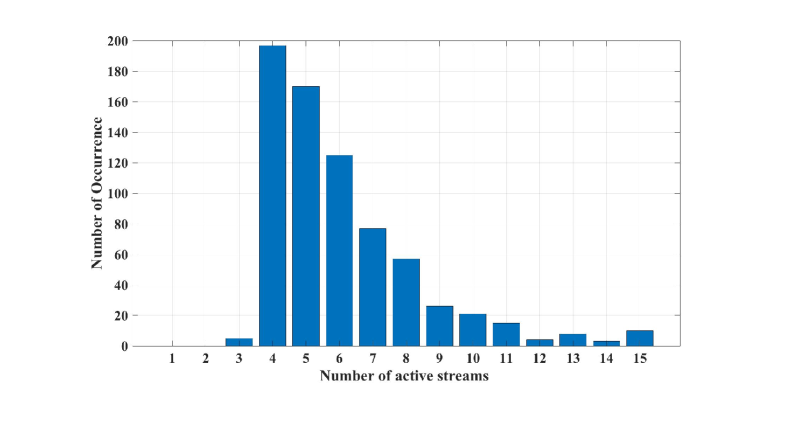
Figure 1: Histogram of the number of active streams to achieve maximum sum rate in the general RS scheme under i.i.d. Rayleigh fading channels, $K=M=4,P=20$ dB.

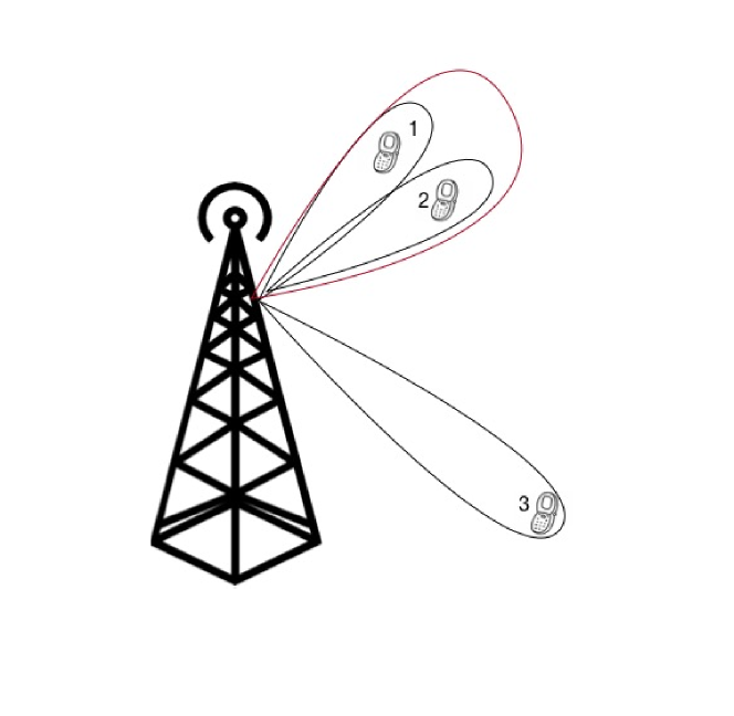
Figure 2: An example to demonstrate the idea that some streams are redundant.

In this subsection, our goal is to find an efficient way to identify a “small” number of “good” streams. We propose a stream selection algorithm, which consists of two steps. The first step is to reduce the number of streams from $2^{K}-1$ to a relatively small number. In the second step, from the remaining streams returned by the first step, we further select maximum non-overlapping collections of streams. Maximum non-overlapping collection will be defined in detail later. This stream selection algorithm considerably facilitates the implementation of successive decoding.

In the first step, we apply the stream elimination algorithm (SEA) in [8] to reduce the number of streams to smaller than $N_{\text{SEA}}$ in total. SEA has been proposed to eliminate some of the streams without losing more than a constant number of bits PCU. Alternatively, SEA provides a way to gradually eliminate the streams so as to identify a given number of remaining streams. This is practically relevant since the number of remaining streams represents the level of precoding/decoding complexity. Let the collection $\bm{\mathcal{S}}$ be the set of the remaining streams returned by SEA.

Claim 3.

If the set $\bm{\mathcal{S}}$ guarantees that the original rate region (without stream elimination) is achievable to within $N$ bits PCU, then the original sum rate, weighted sum rate, and worst-user rate are achievable to within $KN$, $\sum_{k}w_{k}N$, and $N$ bits PCU, respectively.

Proof.

From the assumption, if a rate tuple $(R_{1},\ldots,R_{K})$ is achievable without stream elimination, then $(R_{1}-N,\ldots,R_{K}-N)$ is achievable with the streams in $\bm{\mathcal{S}}$. Then, the conclusion is straightforward. ∎

The above claim implies that if SEA has some performance guarantee in terms of rate gap, then a similar rate guarantee can be obtained in terms of the rate functions of our interest. Since the rate gap is an upper bound, it may appear large for practical uses. Nevertheless, our numerical results show that such guarantee provides meaningful improvement even in practical scenarios.

In the second step, we further select maximum non-overlapping collections of $\bm{\mathcal{S}}$. Without loss of generality, $\bm{\mathcal{S}}$ can be partitioned according to the cardinality of the sets inside it, namely,

$$\bm{\mathcal{S}}=\bigcup_{k=1}^{K}\bm{\mathcal{S}}_{k},$$ (29)

where $\bm{\mathcal{S}}_{k}$ only contains sets of cardinality $k$. We also refer to $\bm{\mathcal{S}}_{k}$ as layer $k$ streams in the following. Let $\tilde{\bm{\mathcal{S}}}\subseteq\bm{\mathcal{S}}$ be a sub-collection, and let us also partition $\tilde{\bm{\mathcal{S}}}$ according to the cardinality of its sets, i.e., $\tilde{\bm{\mathcal{S}}}=\bigcup_{k=1}^{K}\tilde{\bm{\mathcal{S}}}_{k}$. We are interested in $\tilde{\bm{\mathcal{S}}}$ such that $\tilde{\bm{\mathcal{S}}}_{k}$ is a maximum non-overlapping collection of the sets of $\bm{\mathcal{S}}_{k}$, for all $k\in[K]$.

Definition 1.

For all $k\in[K]$, $\tilde{\bm{\mathcal{S}}}_{k}$ is a maximum non-overlapping collection of the sets of $\bm{\mathcal{S}}_{k}$, if the following constraints are satisfied

• ${\mathcal{K}}_{1}\cap{\mathcal{K}}_{2}=\emptyset$, for any distinct sets ${\mathcal{K}}_{1}$ and ${\mathcal{K}}_{2}$ in $\tilde{\bm{\mathcal{S}}}_{k}$;

• if $\hat{\bm{\mathcal{S}}}_{k}:=\bm{\mathcal{S}}_{k}\setminus\tilde{\bm{\mathcal{S}}}_{k}\neq\emptyset$, then ${\mathcal{K}}_{1}\cap{\mathcal{K}}_{2}\neq\emptyset$ for some ${\mathcal{K}}_{1}\in\tilde{\bm{\mathcal{S}}}_{k}$ and ${\mathcal{K}}_{2}\in\hat{\bm{\mathcal{S}}}_{k}$.

It is possible that there are more than one maximum non-overlapping collection for each layer. Let $D_{k}$ denote the number of maximum non-overlapping collections for $\bm{\mathcal{S}}_{k}$, for all $k\in[K]$. Then there are $\prod_{k}D_{k}$ different $\tilde{\bm{\mathcal{S}}}$ in total, which are assembled in $\bm{\mathcal{U}}$. Each $\tilde{\bm{\mathcal{S}}}$ suggests a possible set of active streams for transmission. Algorithm 3 summarizes the above two-step stream selection procedure. Now let us focus on solving ${\mathcal{P}}_{\text{SR}}^{\text{SD}}$ for a given $\tilde{\bm{\mathcal{S}}}$. For each $\tilde{\bm{\mathcal{S}}}\in\bm{\mathcal{U}}$, the following claim can be easily shown.

Algorithm 3 Stream Selection Algorithm

1:  Set a target number $N_{\text{SEA}}$ and use SEA in [8] to reduce the $2^{K}-1$ streams to at most $N_{\text{SEA}}$ streams, denoted by the collection $\bm{\mathcal{S}}$.

2:  Construct $\bm{\mathcal{S}}_{k},k\in[K],$ by partitioning $\bm{\mathcal{S}}$ according to (29).

3:  For all $k\in[K]$, construct the set of $D_{k}$ possible maximum non-overlapping collections $\tilde{\bm{\mathcal{S}}}_{k}$, denoted by ${\bm{\mathcal{U}}}_{k}$.

4:  Assemble the $\prod_{k}D_{k}$ possible $\tilde{\bm{\mathcal{S}}}$ in the set ${\bm{\mathcal{U}}}=\left\{\bigcup_{k=1}^{K}\tilde{\bm{\mathcal{S}}}_{k}|\tilde{\bm{\mathcal{S}}}_{k}\in{\bm{\mathcal{U}}}_{k},k\in[K]\right\}$.

Claim 4.

For all $k\in[K]$, let $\tilde{\bm{\mathcal{K}}}^{(k)}:={\bm{\mathcal{K}}}^{(k)}\cap\tilde{\bm{\mathcal{S}}}$ where ${\bm{\mathcal{K}}}^{(k)}:=\{{\mathcal{K}}\subseteq[K]:\,k\in{\mathcal{K}}\}$ and $\tilde{\bm{\mathcal{S}}}$ is a maximum non-overlapping collection. Then, $|{\mathcal{K}}_{1}|\neq|{\mathcal{K}}_{2}|$ for any distinct sets ${\mathcal{K}}_{1}$ and ${\mathcal{K}}_{2}$ in $\tilde{\bm{\mathcal{K}}}^{(k)}$.

Note that each user $k\in[K]$ only needs to decode the streams in $\tilde{\bm{\mathcal{K}}}^{(k)}$. According to the above claim, there is at most one stream per layer, which implies that each user can decode all the streams successively with the following rule.

Successive decoding rule.

For all $k\in[K]$, let ${\mathcal{K}}_{1},{\mathcal{K}}_{2},\ldots\in\tilde{\bm{\mathcal{K}}}^{(k)}:={\bm{\mathcal{K}}}^{(k)}\cap\tilde{\bm{\mathcal{S}}}$ be ordered with descending cardinality. Then user $k$ decodes the streams ${\mathcal{K}}_{1},{\mathcal{K}}_{2},\ldots$ in order.

Let us introduce the notation $\boldsymbol{\tilde{\pi}}^{(k)}_{\tilde{\bm{\mathcal{S}}}}$ to specify the above unique decoding order at user $k$ for a given $\tilde{\bm{\mathcal{S}}}$. We further define the decoding order $\boldsymbol{\tilde{\pi}}_{\tilde{\bm{\mathcal{S}}}}:=\left(\boldsymbol{\tilde{\pi}}^{(k)}_{\tilde{\bm{\mathcal{S}}}}\right)_{k\in[K]}$, which is particular for the given $\tilde{\bm{\mathcal{S}}}$ since each element $\boldsymbol{\tilde{\pi}}^{(k)}_{\tilde{\bm{\mathcal{S}}}}$ is unique. Therefore, for each possible $\tilde{\bm{\mathcal{S}}}$, we can solve ${\mathcal{P}}_{\text{SR}}^{\text{SD}}(\boldsymbol{\tilde{\pi}}_{\tilde{\bm{\mathcal{S}}}})$ with $\tilde{\bm{\mathcal{K}}}^{(k)}:=\bm{\mathcal{K}}^{(k)}\cap\tilde{\bm{\mathcal{S}}}$ replacing $\bm{\mathcal{K}}^{(k)}$ using CCCP, and return a stationary point. By now, we can summarize the details for solving ${\mathcal{P}}_{\text{SR}}^{\text{SD}}$ with the proposed stream selection in Algorithm 4. The following example can help clarify the above stream selection and successive decoding rule.

Algorithm 4 Solving ${\mathcal{P}}_{\text{SR}}^{\text{SD}}$ with The Proposed Stream Selection

1:  Generate $\bm{\mathcal{U}}$ according to Algorithm 3.

2:  Set $R_{\text{SR}}^{\diamond}$=0.

3:  for each $\tilde{\bm{\mathcal{S}}}\in\bm{\mathcal{U}}$ do

4:     repeat

5:        Obtain an optimal solution of ${\mathcal{P}}_{\text{SR}}^{\text{SD}}(\boldsymbol{\tilde{\pi}}_{\tilde{\bm{\mathcal{S}}}},i)$ with $\tilde{\bm{\mathcal{K}}}^{(k)}:=\bm{\mathcal{K}}^{(k)}\cap\tilde{\bm{\mathcal{S}}}$ replacing $\bm{\mathcal{K}}^{(k)}$, denoted by $\{(\boldsymbol{Q}(i),\tilde{\boldsymbol{R}}(i))\}$, with an interior point method.

6:        Set $i=i+1$.

7:     until the convergence criterion $J_{\text{SR}}(i)\leq\epsilon$ is met.

8:     if $\sum_{{\mathcal{K}}\subseteq[K]}{R}_{{\mathcal{K}}}(i-1)>R_{\text{SR}}^{\diamond}$ then

9:        Set $R_{\text{SR}}^{\diamond}=\sum_{{\mathcal{K}}\subseteq[K]}{R}_{{\mathcal{K}}}(i-1)$, $\boldsymbol{Q}^{\diamond}=\boldsymbol{Q}(i-1)$, $\tilde{\boldsymbol{R}}^{\diamond}=\tilde{\boldsymbol{R}}(i-1)$, $\tilde{\bm{\mathcal{S}}}^{\diamond}=\tilde{\bm{\mathcal{S}}}$ and $\boldsymbol{\pi}^{\diamond}=\boldsymbol{\tilde{\pi}}_{\tilde{\bm{\mathcal{S}}}}$.

10:     end if

11:  end for

Example 1.

Let us consider an example with $K=5$ users. Assume that the initial collection ${\bm{\mathcal{S}}}$ returned by SEA is

$$\bm{\mathcal{S}}=\bigl{\{}\{1\},\{2\},\{3\},\{4\},\{5\},\{1,2\},\{2,3\},\{3,4\},\{4,5\},\{1,2,3\},\{3,4,5\}\bigr{\}}.$$

Therefore, $\bm{\mathcal{S}}$ can be partitioned as in (29) with

$$\bm{\mathcal{S}}_{1}=\bigl{\{}\{1\},\{2\},\{3\},\{4\},\{5\}\bigr{\}},\quad\bm{\mathcal{S}}_{2}=\bigl{\{}\{1,2\},\{2,3\},\{3,4\},\{4,5\}\bigr{\}},$$

$$\bm{\mathcal{S}}_{3}=\bigl{\{}\{1,2,3\},\{3,4,5\}\bigr{\}},\qquad\quad\bm{\mathcal{S}}_{4}=\bm{\mathcal{S}}_{5}=\emptyset.$$

Based on Definition 1, we can verify that the maximum non-overlapping collection $\tilde{\bm{\mathcal{S}}}_{1}$ is ${\bm{\mathcal{S}}}_{1}$ itself. Hence, ${\bm{\mathcal{U}}}_{1}=\tilde{\bm{\mathcal{S}}}_{1}=\bm{\mathcal{S}}_{1}$ and $D_{1}=1$. Next, we put the $D_{2}=3$ possible maximum non-overlapping collections $\tilde{\bm{\mathcal{S}}}_{2}$ in ${\bm{\mathcal{U}}}_{2}$:

$${\bm{\mathcal{U}}}_{2}=\biggl{\{}\bigl{\{}\{1,2\},\{3,4\}\bigr{\}},\quad\bigl{\{}\{2,3\},\{4,5\}\bigr{\}},\quad\bigl{\{}\{1,2\},\{4,5\}\bigr{\}}\biggr{\}}.$$

Similarly, there are $D_{3}=2$ possible maximum non-overlapping collections $\tilde{\bm{\mathcal{S}}}_{3}$ in ${\bm{\mathcal{U}}}_{3}$:

$${\bm{\mathcal{U}}}_{3}=\biggl{\{}\bigl{\{}\{1,2,3\}\bigr{\}},\quad\bigl{\{}\{3,4,5\}\bigr{\}}\biggr{\}}.$$

As a result, there are $D_{1}D_{2}D_{3}=6$ possible maximum non-overlapping collections of $\bm{\mathcal{S}}$ in ${\bm{\mathcal{U}}}$:

$${\bm{\mathcal{U}}}=\left\{\bigcup_{k=1}^{3}\tilde{\bm{\mathcal{S}}}_{k}|\tilde{\bm{\mathcal{S}}}_{k}\in{\bm{\mathcal{U}}}_{k},k=1,2,3\right\}.$$ (30)

Let us consider $\tilde{\bm{\mathcal{S}}}=\{\{1\},\{2\},\{3\},\{4\},\{5\},\{1,2\},\{3,4\},\{1,2,3\}\}\in\bm{\mathcal{U}}$ without loss of generality. User 1 has to decode the streams in ${\bm{\mathcal{K}}}^{(1)}\cap\tilde{\bm{\mathcal{S}}}=\{\{1\},\{1,2\},\{1,2,3\}\}$. This can be done in order $\boldsymbol{\tilde{\pi}}^{(1)}_{\tilde{\bm{\mathcal{S}}}}:\{1,2,3\}\to\{1,2\}\to\{1\}$ according to decreasing cardinality of the sets. Similarly, user 2 decodes in order $\boldsymbol{\tilde{\pi}}^{(2)}_{\tilde{\bm{\mathcal{S}}}}:\{1,2,3\}\to\{1,2\}\to\{2\}$; user 3 decodes in order $\boldsymbol{\tilde{\pi}}^{(3)}_{\tilde{\bm{\mathcal{S}}}}:\{1,2,3\}\to\{3,4\}\to\{3\}$; user 4 decodes in order $\boldsymbol{\tilde{\pi}}^{(4)}_{\tilde{\bm{\mathcal{S}}}}:\{3,4\}\to\{4\}$; user 5 decodes $\{5\}$. Note that for any of the six collections $\tilde{\bm{\mathcal{S}}}\in\bm{\mathcal{U}}$, one can apply the same procedure, and finally return the best collection $\tilde{\bm{\mathcal{S}}}^{\diamond}$ with the highest rate $R_{\text{SR}}^{\diamond}$.

Remark IV.1.

If the users decode the streams with increasing cardinality order instead, each user first decodes its own private message followed by the common messages. In such case, to mitigate the interference while decoding the private message, the power allocated to common messages is likely to be suppressed under noise level, and the benefit of the general RS is therefore not fully exploited.

The proposed stream selection algorithm essentially reduces the number of active streams and removes the excessive search over the decoding order. However, stream selection itself adds extra complexity. Thus, we would like to investigate on the overall complexity of Algorithm 4, i.e., solve ${\mathcal{P}}_{\text{SR}}^{\text{SD}}$ with the proposed stream selection algorithm. Algorithm 4 consists of three parts, 1) perform SEA, 2) select different $\tilde{\bm{\mathcal{S}}}$ and assemble them in $\tilde{\bm{\mathcal{U}}}$, 3) solve ${\mathcal{P}}_{\text{SR}}^{\text{SD}}(\boldsymbol{\tilde{\pi}}_{\tilde{\bm{\mathcal{S}}}})$ for each $\tilde{\bm{\mathcal{S}}}$. The complexity of applying SEA to reduce the $2^{K}-1$ streams to at most $N_{\text{SEA}}$ streams is $\mathcal{O}(KM^{2}2^{K})$ [8]. Then to find all the possible $\tilde{\bm{\mathcal{S}}}$, we can first establish a lookup table offline for a sufficiently large $K$. As long as $N_{\text{SEA}}\leq 2^{K}-1$, we can construct $\tilde{\bm{\mathcal{U}}}$ by searching in the table, regardless of the channel realization. Therefore, the complexity of finding different $\tilde{\bm{\mathcal{S}}}$ can be neglected. The complexity of the third step involves the complexity of solving ${\mathcal{P}}_{\text{SR}}^{\text{SD}}(\boldsymbol{\tilde{\pi}}_{\tilde{\bm{\mathcal{S}}}})$ for all $\tilde{\bm{\mathcal{S}}}$. However, it is hard to characterize the exact value of $D_{k}$ for an arbitrary $N_{\text{SEA}}$ in general. The difficulty comes from the unknown overlap among the remaining streams after SEA. Therefore, we present an upper bound on the complexity for this part. For a given $\tilde{\bm{\mathcal{S}}}$, ${\mathcal{P}}_{\text{SR}}^{\text{SD}}(\boldsymbol{\tilde{\pi}}_{\tilde{\bm{\mathcal{S}}}})$ is a convex problem with at most $(M^{2}+1)N_{\text{SEA}}$ variables and $1+(K+1)N_{\text{SEA}}$ constraints. Therefore, the worst-case complexity for solving ${\mathcal{P}}_{\text{SR}}^{\text{SD}}(\boldsymbol{\tilde{\pi}}_{\tilde{\bm{\mathcal{S}}}})$ for a given $\tilde{\bm{\mathcal{S}}}$ using CCCP is $\mathcal{O}\left(M^{6}N_{\text{SEA}}^{3.5}K^{0.5}\right)$. Next, to characterize $D_{k}$, we consider all the streams of layer $k$, i.e., $\binom{K}{k}$ in total, if there exists at least one layer-$k$ stream after SEA. Note that such calculation may incorporate several streams already eliminated by SEA, and hence leads to an upper bound. Let $k^{*}({N_{\text{SEA}}})$ denote the smallest $k$ such that $\sum_{k^{\prime}=1}^{k}\binom{K}{k^{\prime}}\geq N_{\text{SEA}}$. Then the number of possible $\tilde{\bm{\mathcal{S}}}$ is no greater than $\prod_{k=2}^{k^{*}({N_{\text{SEA}}})}\frac{\binom{K}{k}\binom{K-k}{k}\cdots\binom{K-(\lfloor\frac{K}{k}\rfloor-1)\times k}{k}}{\lfloor\frac{K}{k}\rfloor\times\max{(1,\lfloor\frac{K}{k}\rfloor-1)}}$, which can be further upper bounded by $\binom{K}{K/2}^{\frac{N_{\text{SEA}}}{2}}$. As a result, the worst-case complexity of solving ${\mathcal{P}}_{\text{SR}}^{\text{SD}}$ with the proposed stream selection is $\mathcal{O}\left(KM^{2}2^{K}+M^{6}N_{\text{SEA}}^{3.5}K^{0.5}\binom{K}{K/2}^{\frac{N_{\text{SEA}}}{2}}\right)$. The above calculation is omitted for brevity. Let us consider $M=K=4$, then the complexity of solving ${\mathcal{P}}_{\text{SR}}^{\text{SD}}$ without stream selection is about $10^{26}$, while the upper bound on the worst-case complexity of solving ${\mathcal{P}}_{\text{SR}}^{\text{SD}}$ with our stream selection is about $10^{8}$ if $N_{\text{SEA}}=6$. The above comparison suggests that the complexity of precoder design after our stream selection algorithm is considerably reduced.

IV-C Imperfect CSIT

In practice, the CSIT is obtained by direct estimation or limited feedback from the receivers. Therefore, the information may be inaccurate or outdated. A common model for imperfect CSIT is to assume that

$$\boldsymbol{\mathsf{H}}=\hat{\boldsymbol{\mathsf{H}}}+\tilde{\boldsymbol{\mathsf{H}}},$$ (31)

where $\hat{\boldsymbol{\mathsf{H}}}$ is the channel estimate and $\tilde{\boldsymbol{\mathsf{H}}}$ is the estimation error that is unknown to the transmitter, and they are independent. In addition, we assume for simplicity that $\tilde{\boldsymbol{\mathsf{H}}}$ has i.i.d. entries with variance $\sigma^{2}$ each. Let $\hat{{\boldsymbol{H}}}$ be a particular realization of $\hat{\boldsymbol{\mathsf{H}}}$. The precoder design should only depend on the estimate $\hat{{\boldsymbol{H}}}$ and the CSIT inaccuracy.

A proper way to characterize the performance with imperfect CSIT is the outage formulation, e.g., to find out the achievable rate tuples for a given outage probability. But it is hard to derive closed-form expressions exploitable for precoder optimization. Therefore, instead of reformulating entirely the problem with imperfect CSIT, we seek an adaptation of the one derived for perfect CSIT. To that end, we adopt an ergodic formulation which replaces (14) with the following constraint

$$\sum_{\mathcal{K}\in\bm{\mathcal{S}}^{(k)}}{R}_{\mathcal{K}}\leq\mathbb{E}_{\tilde{\boldsymbol{\mathrm{H}}}_{k}}\left\{\log\biggl{(}1+\frac{\sum_{\mathcal{K}\in\bm{\mathcal{S}}^{(k)}}\boldsymbol{\mathrm{H}}_{k}^{\scriptscriptstyle\mathsf{H}}{\boldsymbol{Q}}_{\mathcal{K}}\boldsymbol{\mathrm{H}}_{k}}{1+\sum_{\mathcal{K}^{\prime}\not\in{\bm{\mathcal{K}}}^{(k)}}\boldsymbol{\mathrm{H}}_{k}^{\scriptscriptstyle\mathsf{H}}{\boldsymbol{Q}}_{\mathcal{K}^{\prime}}\boldsymbol{\mathrm{H}}_{k}}\biggr{)}\right\},\quad\forall\,k\in[K],\bm{\mathcal{S}}^{(k)}\subseteq\bm{\mathcal{K}}^{(k)},$$ (32)

where $\boldsymbol{\mathrm{H}}_{k}:=\hat{{\boldsymbol{h}}}_{k}+\tilde{\boldsymbol{\mathrm{H}}}_{k}$ is the random channel vector; and the expectation is over the CSI error. Note that in the above expression, we implicitly assume that the random channel vector is known at the receivers, whereas only the expectation on the right-hand side of (32) is known at the transmitter’s side. Such formulation is also widely used in the literature of robust optimization [27, 34]. There are two issues with the above formulation though. First, we need to know the exact distribution of the CSI error to compute the expectation. This may not be possible in practice. Second, even with the exact distribution, finding the expectation can be computationally costly. In order to capture the CSI error in a simple way, we work with a lower bound on the expectation on the right-hand side of (32).

Claim 5.

If the CSI error is symmetrically distributed such that $-\tilde{\boldsymbol{\mathsf{H}}}$ has the same distribution as $\tilde{\boldsymbol{\mathsf{H}}}$, then we have the following lower bound on the expectation

$$\mathbb{E}_{\tilde{\boldsymbol{\mathrm{H}}}_{k}}\left\{\log\biggl{(}1+\frac{\sum_{\mathcal{K}\in\bm{\mathcal{S}}^{(k)}}\boldsymbol{\mathrm{H}}_{k}^{\scriptscriptstyle\mathsf{H}}{\boldsymbol{Q}}_{\mathcal{K}}\boldsymbol{\mathrm{H}}_{k}}{1+\sum_{\mathcal{K}^{\prime}\not\in{\bm{\mathcal{K}}}^{(k)}}\boldsymbol{\mathrm{H}}_{k}^{\scriptscriptstyle\mathsf{H}}{\boldsymbol{Q}}_{\mathcal{K}^{\prime}}\boldsymbol{\mathrm{H}}_{k}}\biggr{)}\right\}\\ \geq\log\biggl{(}1+\frac{\sum_{\mathcal{K}\in\bm{\mathcal{S}}^{(k)}}\hat{{\boldsymbol{h}}}_{k}^{\scriptscriptstyle\mathsf{H}}{\boldsymbol{Q}}_{\mathcal{K}}\hat{{\boldsymbol{h}}}_{k}}{1+\sum_{\mathcal{K}^{\prime}\not\in{\bm{\mathcal{K}}}^{(k)}}\bigl{(}\hat{{\boldsymbol{h}}}_{k}^{\scriptscriptstyle\mathsf{H}}{\boldsymbol{Q}}_{\mathcal{K}^{\prime}}\hat{{\boldsymbol{h}}}_{k}+\sigma^{2}\text{tr}\left(\right)({\boldsymbol{Q}}_{\mathcal{K}^{\prime}})\bigr{)}}\biggr{)},\quad\forall\,k\in[K],\bm{\mathcal{S}}^{(k)}\subseteq\bm{\mathcal{K}}^{(k)}.$$ (35)

Proof.

The expectation can be rewritten as the difference of two expectations, i.e.,

$$\mathbb{E}_{\tilde{\boldsymbol{\mathrm{H}}}_{k}}\left\{\log\biggl{(}1+\frac{\sum_{\mathcal{K}\in\bm{\mathcal{S}}^{(k)}}\boldsymbol{\mathrm{H}}_{k}^{\scriptscriptstyle\mathsf{H}}{\boldsymbol{Q}}_{\mathcal{K}}\boldsymbol{\mathrm{H}}_{k}}{1+\sum_{\mathcal{K}^{\prime}\not\in{\bm{\mathcal{K}}}^{(k)}}\boldsymbol{\mathrm{H}}_{k}^{\scriptscriptstyle\mathsf{H}}{\boldsymbol{Q}}_{\mathcal{K}^{\prime}}\boldsymbol{\mathrm{H}}_{k}}\biggr{)}\right\}\\ =\mathbb{E}_{\tilde{\boldsymbol{\mathrm{H}}}_{k}}\!\!\left\{\log\left(1+\boldsymbol{\mathrm{H}}_{k}^{\scriptscriptstyle\mathsf{H}}\left(\sum_{\mathcal{K}^{\prime}\not\in{\bm{\mathcal{K}}}^{(k)}}\!\!{\boldsymbol{Q}}_{\mathcal{K}^{\prime}}+\!\!\!\!\sum_{\mathcal{K}\in\bm{\mathcal{S}}^{(k)}}\!\!{\boldsymbol{Q}}_{\mathcal{K}}\right)\right)\!\boldsymbol{\mathrm{H}}_{k}\!\right\}-\mathbb{E}_{\tilde{\boldsymbol{\mathrm{H}}}_{k}}\!\!\left\{\log\left(1+\!\!\sum_{\mathcal{K}^{\prime}\not\in{\bm{\mathcal{K}}}^{(k)}}\boldsymbol{\mathrm{H}}_{k}^{\scriptscriptstyle\mathsf{H}}{\boldsymbol{Q}}_{\mathcal{K}^{\prime}}\boldsymbol{\mathrm{H}}_{k}\right)\right\},$$ (38)

where the second term can be upper bounded with Jensen’s inequality as

$$\mathbb{E}_{\tilde{\boldsymbol{\mathrm{H}}}_{k}}\left\{\log\left(1+\sum_{\mathcal{K}^{\prime}\not\in{\bm{\mathcal{K}}}^{(k)}}\boldsymbol{\mathrm{H}}_{k}^{\scriptscriptstyle\mathsf{H}}{\boldsymbol{Q}}_{\mathcal{K}^{\prime}}\boldsymbol{\mathrm{H}}_{k}\right)\right\}\leq\log\biggl{(}1+\sum_{\mathcal{K}^{\prime}\not\in{\bm{\mathcal{K}}}^{(k)}}\bigl{(}\hat{{\boldsymbol{h}}}_{k}^{\scriptscriptstyle\mathsf{H}}{\boldsymbol{Q}}_{\mathcal{K}^{\prime}}\hat{{\boldsymbol{h}}}_{k}+\sigma^{2}\text{tr}\left(\right)({\boldsymbol{Q}}_{\mathcal{K}^{\prime}})\bigr{)}\biggr{)}.$$ (39)

Next, we look at the first term on the right-hand side of (38). We consider a simple form of it as

$$f(\sigma):=\mathbb{E}_{\boldsymbol{\mathrm{G}}}\left\{\log(1+(\hat{{\boldsymbol{h}}}+\sigma\boldsymbol{\mathrm{G}})^{\scriptscriptstyle\mathsf{H}}{\boldsymbol{A}}(\hat{{\boldsymbol{h}}}+\sigma\boldsymbol{\mathrm{G}}))\right\},$$ (40)

where the random vector $\sigma\boldsymbol{\mathrm{G}}$ has the same distribution as $\tilde{\boldsymbol{\mathrm{H}}}_{k}$; ${\boldsymbol{A}}$ is some positive semi-definite matrix. To prove the claim, it is enough to show that $f(\sigma)$ defined above is non-decreasing with $\sigma$. To that end, let us take the first derivative of $f(\sigma)$.

$$\frac{\mathrm{d}f(\sigma)}{\mathrm{d}\sigma} =\log e\cdot\mathbb{E}_{\boldsymbol{\mathrm{G}}}\left\{\frac{2\sigma\boldsymbol{\mathrm{G}}^{\scriptscriptstyle\mathsf{H}}{\boldsymbol{A}}\boldsymbol{\mathrm{G}}+2\mathrm{Re}\{\boldsymbol{\mathrm{G}}^{\scriptscriptstyle\mathsf{H}}{\boldsymbol{A}}\hat{{\boldsymbol{h}}}\}}{1+(\hat{{\boldsymbol{h}}}+\sigma\boldsymbol{\mathrm{G}})^{\scriptscriptstyle\mathsf{H}}{\boldsymbol{A}}(\hat{{\boldsymbol{h}}}+\sigma\boldsymbol{\mathrm{G}})}\right\}$$ (41)

$$\geq\log e\cdot\mathbb{E}_{\boldsymbol{\mathrm{G}}}\left\{\frac{2\mathrm{Re}\{\boldsymbol{\mathrm{G}}^{\scriptscriptstyle\mathsf{H}}{\boldsymbol{A}}\hat{{\boldsymbol{h}}}\}}{1+(\hat{{\boldsymbol{h}}}+\sigma\boldsymbol{\mathrm{G}})^{\scriptscriptstyle\mathsf{H}}{\boldsymbol{A}}(\hat{{\boldsymbol{h}}}+\sigma\boldsymbol{\mathrm{G}})}\right\}$$ (42)

$$\geq\log e\cdot\mathbb{E}_{\boldsymbol{\mathrm{G}}}\left\{\frac{2\mathrm{Re}\{\boldsymbol{\mathrm{G}}^{\scriptscriptstyle\mathsf{H}}{\boldsymbol{A}}\hat{{\boldsymbol{h}}}\}}{1+\max_{b\in\{1,-1\}}\left\{(\hat{{\boldsymbol{h}}}+b\sigma\boldsymbol{\mathrm{G}})^{\scriptscriptstyle\mathsf{H}}{\boldsymbol{A}}(\hat{{\boldsymbol{h}}}+b\sigma\boldsymbol{\mathrm{G}})\right\}}\right\}$$ (43)

$$=0$$ (44)

where (41) is obtained by putting the derivative inside the expectation; (42) comes from the fact that ${\boldsymbol{A}}$ is positive semi-definite, i.e., $\boldsymbol{\mathrm{G}}^{\scriptscriptstyle\mathsf{H}}{\boldsymbol{A}}\boldsymbol{\mathrm{G}}\geq 0$ with probability $1$; we introduced $b\in\{1,-1\}$ to obtain the lower bound (43) and to symmetrize the denominator with respect to $\boldsymbol{\mathrm{G}}$; the last equality is from the fact that $\boldsymbol{\mathrm{G}}$ is symmetrically distributed and that the function inside the expectation is odd with respect to $\boldsymbol{\mathrm{G}}$. Indeed, for any odd function $g(\cdot)$, we have $\mathbb{E}\left\{g(\boldsymbol{\mathrm{G}})\right\}=\mathbb{E}\left\{g(-\boldsymbol{\mathrm{G}})\right\}=-\mathbb{E}\left\{g(\boldsymbol{\mathrm{G}})\right\}$ due to the symmetry of the distribution of $\boldsymbol{\mathrm{G}}$ and the symmetry of the function, respectively. This leads to $\mathbb{E}\left\{g(\boldsymbol{\mathrm{G}})\right\}=0$. ∎

Note that the symmetry of the CSI error is a mild assumption that can be satisfied in practical situations. Therefore, to take into account the CSI inaccuracy for joint decoding, we propose to replace (14) with the following constraint

$$\sum_{\mathcal{K}\in\bm{\mathcal{S}}^{(k)}}{R}_{\mathcal{K}}\leq\log\biggl{(}1+\frac{\sum_{\mathcal{K}\in\bm{\mathcal{S}}^{(k)}}\hat{{\boldsymbol{h}}}_{k}^{\scriptscriptstyle\mathsf{H}}{\boldsymbol{Q}}_{\mathcal{K}}\hat{{\boldsymbol{h}}}_{k}}{1+\sum_{\mathcal{K}^{\prime}\not\in{\bm{\mathcal{K}}}^{(k)}}\bigl{(}\hat{{\boldsymbol{h}}}_{k}^{\scriptscriptstyle\mathsf{H}}{\boldsymbol{Q}}_{\mathcal{K}^{\prime}}\hat{{\boldsymbol{h}}}_{k}+\sigma^{2}\text{tr}\left(\right)({\boldsymbol{Q}}_{\mathcal{K}^{\prime}})\bigr{)}}\biggr{)},\quad\forall\,k\in[K],\bm{\mathcal{S}}^{(k)}\subseteq\bm{\mathcal{K}}^{(k)}.$$ (45)

Similarly, for successive decoding, we can replace (25) with the following constraint

$${R}_{{\mathcal{K}}^{(k)}_{\pi_{k,n}}}\leq$$

$$\log\biggl{(}1+\frac{\hat{{\boldsymbol{h}}}_{k}^{H}{\boldsymbol{Q}}_{{\mathcal{K}}^{(k)}_{\pi_{k,n}}}\hat{{\boldsymbol{h}}}_{k}}{1+\sum_{{{\mathcal{K}}^{\prime}}\not\in\bm{\mathcal{K}}^{(k)}}\bigl{(}\hat{{\boldsymbol{h}}}_{k}^{H}{\boldsymbol{Q}}_{{{\mathcal{K}}^{\prime}}}\hat{{\boldsymbol{h}}}_{k}+\sigma^{2}\text{tr}\left(\right)({\boldsymbol{Q}}_{\mathcal{K}^{\prime}})\bigr{)}+\sum_{n^{\prime}>n}\bigl{(}\hat{{\boldsymbol{h}}}_{k}^{H}{\boldsymbol{Q}}_{{\mathcal{K}}^{(k)}_{\pi_{k,n^{\prime}}}}\hat{{\boldsymbol{h}}}_{k}+\sigma^{2}\text{tr}\left(\right)({\boldsymbol{Q}}_{{\mathcal{K}}^{(k)}_{\pi_{k,n^{\prime}}}})\bigr{)}}\biggr{)}$$

$$\qquad\qquad\qquad\qquad\qquad\qquad\qquad\qquad\qquad\qquad\forall\,k\in[K],n\in[2^{K-1}].$$ (46)

With the above constraints, we can still apply CCCP to solve the precoder design problems under imperfect CSIT, as presented in the Section III and in Section IV-A, since the presences of the CSI error terms in (45) and (46) do not change the convexity of the denominators. Essentially, here we try to optimize some lower bounds of the rate functions over a set of covariance matrices. Then we can apply the precoders returned by the algorithms, and achieve at least as good as the lower bounds predict.

V Numerical Results

In this section, we provide some numerical results to illustrate the performance of the proposed algorithms. While we focus on the sum rate performance in this section, similar conclusions can be obtained for the weighted sum rate, worst-user rate, or minimum power scenarios. Assuming the spatially correlated Rayleigh-fading channel, we have ${\boldsymbol{h}}_{k}\sim\mathcal{CN}(\bm{0},{\boldsymbol{R}}_{k})$, where ${\boldsymbol{R}}_{k}$ is a positive semi-definite channel covariance matrix. With the Karhunen-Loeve representation, the downlink channel ${\boldsymbol{h}}_{k}$ of user $k$ is in the form ${\boldsymbol{h}}_{k}={\boldsymbol{U}}_{k}\bm{\Lambda}_{k}^{\frac{1}{2}}{\boldsymbol{w}}_{k}$, where ${\boldsymbol{w}}_{k}\in\mathbb{C}^{r_{k}\times 1}\sim\mathcal{CN}(\bm{0},{\boldsymbol{\mathrm{I}}})$, $\bm{\Lambda}_{k}$ is an $r_{k}\times r_{k}$ diagonal matrix whose elements are the nonzero eigenvalues of ${\boldsymbol{R}}_{k}$, and ${\boldsymbol{U}}_{k}\in\mathbb{C}^{M\times r_{k}}$ is the tall unitary matrix formed by the corresponding eigenvectors.

We further consider the one-ring scattering model [35]. Then the correlation between the channel coefficients of antennas $1\leq m,p\leq M$ is given by

$$[{\boldsymbol{R}}_{k}]_{m,p}=\frac{1}{2\Delta_{k}}\int_{{\theta_{k}}-{\Delta_{k}}}^{{\theta_{k}}+{\Delta_{k}}}{{e^{-j\frac{2\pi}{\lambda}\bm{\Phi}(\alpha)({\boldsymbol{u}}_{m}-{\boldsymbol{u}}_{p})}}d\alpha},$$ (47)

where $\theta_{k}$ is the azimuth angle of user $k$ with respect to the orientation perpendicular to the array axis, $\Delta_{k}$ indicates the angular spread (AS) of departure to user $k$, $\bm{\Phi}(\alpha)=[\cos(\alpha),\sin(\alpha)]$ is the wave vector for a planar wave impinging with the angle of $\alpha$, $\lambda$ is the wavelength and ${\boldsymbol{u}}_{m}=[x_{m},y_{m}]^{{\scriptscriptstyle\mathsf{T}}}$ is the vector indicating the position of BS antenna $m$ in the 2-D coordinate system. Let us consider the special but important case of a uniform linear array (ULA) placed at the origin along the y-axis. Denoting by $\lambda D$ the spacing of antenna elements, the covariance matrix of the channel is given by the Toeplitz form

$$[{\boldsymbol{R}}_{k}]_{m,p}=\frac{1}{2\Delta_{k}}\int_{{\theta_{k}}-{\Delta_{k}}}^{{\theta_{k}}+{\Delta_{k}}}{{e^{-j2\pi D(m-p)\sin(\alpha)}}d\alpha}.$$ (48)

Suppose that $K$ users are selected to form $G$ groups based on the similarity of their channel covariance matrices. We let $K_{g}$ denote the number of users in group $g$, such that $K=\sum\nolimits_{g=1}^{G}K_{g}$. We make the same assumption as in [35] that users in the same group $g$ share the same covariance matrix ${\boldsymbol{R}}_{g}={\boldsymbol{U}}_{g}\bm{\Lambda}_{g}{\boldsymbol{U}}_{g}$. More precisely, the channel vector of user $k$ in group $g$ is given by ${\boldsymbol{h}}_{k}={\boldsymbol{U}}_{g}\bm{\Lambda}_{g}^{\frac{1}{2}}{\boldsymbol{w}}_{k}$.

The baseline schemes are the following:

• The sum capacity $C_{\text{sum}}$ that can be derived with the MAC-BC duality as

  $$C_{\text{sum}}=\max_{\sum_{i}P_{i}\leq P}\log\text{det}\left(\right)({\boldsymbol{\mathrm{I}}}+{\boldsymbol{H}}^{H}\text{diag}\left(\right)(P_{1},\ldots,P_{K}){\boldsymbol{H}})$$

  The above problem is convex and can be solved efficiently.

• The unicast scheme with the covariance matrices obtained by solving the following problem

  $${\mathcal{P}}_{\text{uni}}:\quad \mathop{\max}\limits_{{\boldsymbol{Q}}_{k}\succeq 0}\sum_{k\in[K]}R_{k}$$

  $$\text{s.t. }\;\eqref{eq:unicast_SINR},\sum_{k\in[K]}\text{tr}\left(\right)\left({\boldsymbol{Q}}_{k}\right)\leq P$$

• The 1-layer RS (the only common message sent by the BS is intended to all the users) with successive decoding [14, 15, 17].

• The ZF scheme with precoder $({\boldsymbol{H}}^{\scriptscriptstyle\mathsf{H}})^{\dagger}\text{diag}\left(\right)\{\sqrt{{\boldsymbol{p}}^{\text{opt}}}\}$ [36], where ${\boldsymbol{p}}^{\text{opt}}$ is the solution to

  $$\max_{{\boldsymbol{p}}\geq 0}\sum_{k}\log(1+p_{k})\;\;\text{s.t. }\sum\nolimits_{k}p_{k}[({\boldsymbol{H}}^{\scriptscriptstyle\mathsf{H}}{\boldsymbol{H}})^{-1}]_{k,k}\leq P.$$ (49)

  We emphasize that, for comparison fairness, we apply a similar CCCP to solve the precoder optimizations for both the unicast scheme and the 1-layer RS scheme. Note that the algorithms proposed in the references for the 1-layer RS do not necessarily consider power optimization for each individual message, resulting a strictly suboptimal solution compared to that obtained with CCCP.

  We first verify the performance of the general RS scheme with joint decoding for a small number of users, i.e., $K=3$. To that end, we assume $G=2$ groups, and each user can be inside any of the clusters with equal probability. We set the azimuth angle of the $g$-th group as $\theta_{g}=-\frac{\pi}{3}+\frac{15\pi}{180}(g-1)$ and assume the same AS for all groups as $\Delta=\frac{5\pi}{180}$. Algorithm 1 is applied to obtain a stationary point of the sum rate of the general RS with joint decoding. It is demonstrated in Fig. 3 that both the 1-layer RS and the general RS considerably increase the sum rate compared to unicast, especially at high SNR. In addition, with only 3 more streams in the general RS, we can improve the sum rate by more than 1 bit compared to the 1-layer RS at medium-high SNR. As the users in the same group have correlated channels, it is reasonable to decode the interference inside the group instead of treating it as noise. Since the users are spatially correlated in the one-ring scattering model, the performance of the ZF scheme degrades severely as demonstrated in Fig. 3. Therefore, in the following, we will not consider ZF.

  

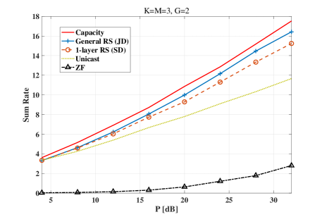
  Figure 3: Comparison of the capacity, sum rates under the general RS (JD), 1-layer RS (SD), unicast and ZF, $K=3,M=3,G=2,\Delta=\frac{5\pi}{180},\theta_{g}=-\frac{\pi}{3}+\frac{15\pi}{180}(g-1)$.

  Now let us adopt Algorithm 4 to solve ${\mathcal{P}}_{\text{SR}}^{\text{SD}}$ with the proposed stream selection for the 4-user case. We set $N_{\text{SEA}}=15$. Thus the first step in Algorithm 3 actually preserves all the $2^{K}-1$ steams. Since each $\tilde{\bm{\mathcal{S}}}$ generated by Algorithm 3 contains $8$ streams instead of the original $15$ streams, the decoding complexity for each user is substantially reduced. Recall that for a given collection $\tilde{\bm{\mathcal{S}}}$, the decoding order is fixed after the stream selection as explained in Section IV-B. We consider two scenarios with disjoint and overlapping eigen-subspaces, respectively, in Fig. 4. We set $\theta_{g}=-\frac{\pi}{3}+\Delta+\frac{15\pi}{180}(g-1)$ and $\Delta=\frac{5\pi}{180}$ for the former scenario, while $\theta_{g}=-\frac{\pi}{3}+\frac{10\pi}{180}(g-1)$ and $\Delta=\frac{15\pi}{180}$ for the latter. In the scenario with disjoint eigen-subspaces, inter-group interference is small and common messages across different groups are not needed, the 1-layer RS boils down to the unicast scheme. It is worth mentioning that in the simulation, the 1-layer RS slightly outperforms the unicast since we randomly put four users in two groups. Therefore, it is possible that all the users are in the same group so that they all benefit from the common message. The general RS after stream selection, which has three additional streams, further improves the sum rate. However, in such disjoint case, extra streams only brings slight intra-group rate increase. In contrast, in the overlapping case, the common message to all the users increases the sum rate by 2 bits compared to unicast. Apart from this, a large gain is further enabled by three additional inter-group common messages in the general RS.

  

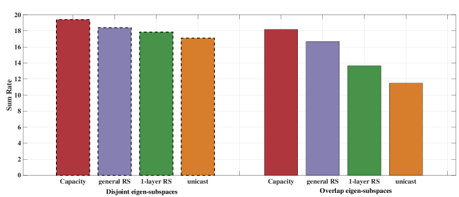
  Figure 4: Comparison of the capacity, the sum rates under the general RS after stream selection (SD), the 1-layer RS scheme (SD), and the unicast scheme. $K=4,M=4,G=2,P=30\,$dB. Two considered scenarios: 1) disjoint eigen-spaces ($\Delta=\frac{5\pi}{180},\theta_{g}=-\frac{\pi}{3}+\Delta+\frac{15\pi}{180}(g-1)$), 2) overlapping eigen-spaces ($\Delta=\frac{15\pi}{180},\theta_{g}=-\frac{\pi}{3}+\frac{10\pi}{180}(g-1)$).

  In Fig. 5, we consider a larger number of users, i.e., $K=8$. In this simulation, we assume that 8 users can be inside any of the two groups with equal probability. We set $\Delta=\frac{20\pi}{180}$ and $\theta_{g}=-\frac{\pi}{3}+\frac{\pi}{8}(g-1)$, which corresponds to overlapping eigen-spaces between the two groups. In this case, the general RS scheme involves 255 streams, which is infeasible due to high complexity. Thanks to the stream selection algorithm, it is possible to investigate the performance of the general RS under such relatively large number of users. We set $N_{\text{SEA}}=38$, then each $\tilde{\bm{\mathcal{S}}}$ generated by Algorithm 3 contains 30 streams. Furthermore, the number of constraints in successive decoding is reduced to 16, which is implementable in practice. Fig. 5 suggests that the 1-layer RS slightly outperforms the unicast, while the general RS further provides a large gain thanks to the use of multiple inter-group common messages. This observation confirms the effectiveness of our stream selection in identifying “good” streams.

  

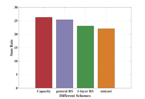
  Figure 5: Comparison of the capacity, the sum rates under the general RS after stream selection (SD), the 1-layer RS scheme (SD), and the unicast scheme. $K=M=8,P=30$dB, $G=2,\Delta=\frac{20\pi}{180},\theta_{g}=-\frac{\pi}{3}+\frac{\pi}{8}(g-1)$.

  Finally, let us consider i.i.d. channels and investigate the performance of the general RS with imperfect CSIT. We assume that $\boldsymbol{\mathsf{H}}=\hat{\boldsymbol{\mathsf{H}}}+\tilde{\boldsymbol{\mathsf{H}}}$ as in (31). Here, we let the entries of $\tilde{\boldsymbol{\mathsf{H}}}$ and $\hat{\boldsymbol{\mathsf{H}}}$ be i.i.d. circularly symmetric Gaussian with variances $\sigma^{2}$ and $1-\sigma^{2}$, respectively. In Fig. 7, the sum rate with the proposed regularization is calculated as follows. We first optimize the sum rate based on the lower bound, i.e., replace the rate constraints in (25) by those in (46) in Algorithm 2, and achieve a group of feasible ${\boldsymbol{Q}}$. Then, we substitute such returned ${\boldsymbol{Q}}$ into the real rate constraints in (25) to get a set of achievable rates, and thus the sum rate. To obtain the sum rate of the general RS without regularization, we solve ${\mathcal{P}}_{\text{SR}}^{\text{SIC}}$ with $\hat{{\boldsymbol{H}}}$ directly replacing ${\boldsymbol{H}}$, and then substitute the returned ${\boldsymbol{Q}}$ into (25) with the real channel matrix ${\boldsymbol{H}}$ to get the achievable rates. The results show that the proposed regularization brings remarkable rate improvement especially when the CSIT error $\sigma^{2}$ is large, e.g., almost up to $200\%$ gain when $\sigma^{2}=0.9$. In Fig.7, we compare the performance of the unicast and the general RS after stream selection. The sum rate of the unicast scheme with regularization is obtained by steps similar to those for the general RS with regularization. We can observe that the general RS always outperforms the unicast scheme even with a large estimation error.

  

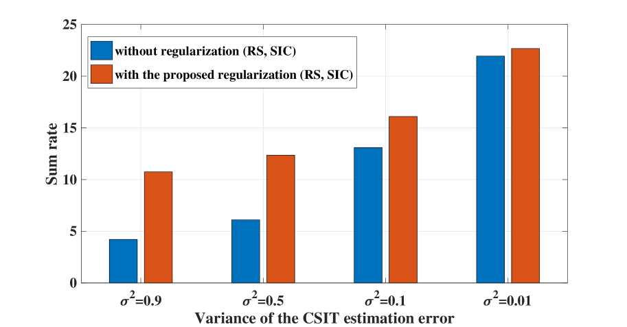
  Figure 6: Sum rate comparisons without and with the proposed regularization, imperfect CSIT, $K=M=4,P=30$dB, $N_{\text{SEA}}=2^{K}-1$, both with the general RS, i.i.d. channels.

  

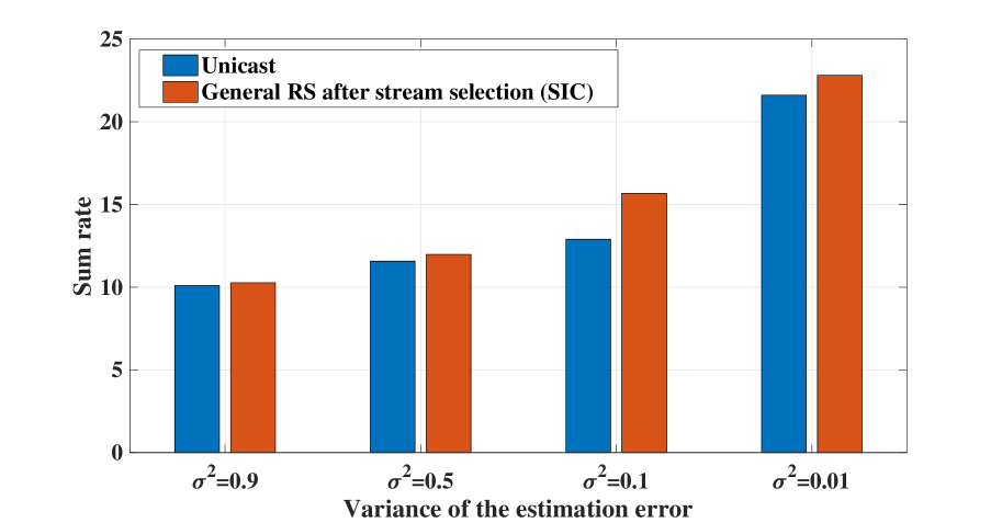
  Figure 7: Sum rate comparisons under the general RS and unicast, both with the proposed regularization, imperfect CSIT, $K=M=4,P=30$dB, $N_{\text{SEA}}=2^{K}-1$, i.i.d. channels.

  VI Conclusion

  In this work, we have investigated the general RS scheme applied for multi-antenna downlink communications. We have proposed a full range of novel solutions including precoder design, stream selection, and imperfect CSIT regularization. We have run numerical simulations showing that our RS solutions, even under practical constraints, can provide substantial performance gains over existing schemes. It is worth noting that since RS is linear, the implementation cost of the proposed algorithms are comparable to those applied in practical systems. In summary, our study has demonstrated that the general RS is a viable way to mitigate interference in future multi-antenna networks.

References

- [1] T. E. Bogale and L. B. Le, “Massive MIMO and mmWave for 5G wireless HetNet: Potential benefits and challenges,” IEEE Veh. Technol. Mag., vol. 11, no. 1, pp. 64–75, Mar. 2016.
- [2] G. Zhu, K. Huang, V. K. Lau, B. Xia, X. Li, and S. Zhang, “Hybrid beamforming via the Kronecker decomposition for the millimeter-wave massive MIMO systems,” IEEE J. Sel. Areas Commun., vol. 35, no. 9, pp. 2097–2114, Sept. 2017.
- [3] G. Caire and S. Shamai (Shitz), “On the achievable throughput of a multiantenna Gaussian broadcast channel,” IEEE Trans. Inf. Theory, vol. 49, no. 7, pp. 1691 – 1706, July 2003.
- [4] H. Weingarten, Y. Steinberg, and S. Shamai (Shitz), “The capacity region of the Gaussian multiple-input multiple-output broadcast channel,” IEEE Trans. Inf. Theory, vol. 52, no. 9, pp. 3936 –3964, Sept. 2006.
- [5] S. Yang and J.-C. Belfiore, “The impact of channel estimation error on the DPC region of the two-user Gaussian broadcast channel,” in Proc. 43rd Allerton Conference, 2005.
- [6] T. Yoo and A. Goldsmith, “On the optimality of multiantenna broadcast scheduling using zero-forcing beamforming,” IEEE J. Sel. Areas Commun., vol. 24, no. 3, pp. 528–541, Mar. 2006.
- [7] J. Lee and N. Jindal, “High SNR analysis for MIMO broadcast channels: Dirty paper coding versus linear precoding,” IEEE Trans. Inf. Theory, vol. 53, no. 12, pp. 4787–4792, Dec. 2007.
- [8] Z. Li, S. Yang, and S. Shamai (Shitz), “On linearly precoded rate splitting for MIMO broadcast channels,” Available on arXiv:1808.01810.
- [9] A. Carleial, “Interference channels,” IEEE Trans. Inf. Theory, vol. 24, no. 1, pp. 60–70, Jan. 1978.
- [10] T. S. Han and K. Kobayashi, “A new achievable rate region for the interference channel,” IEEE Trans. Inf. Theory, vol. 27, no. 1, pp. 49 – 60, Jan. 1981.
- [11] R. H. Etkin, D. N. C. Tse, and H. Wang, “Gaussian interference channel capacity to within one bit,” IEEE Trans. Inf. Theory, vol. 54, no. 12, pp. 5534–5562, Dec. 2008.
- [12] S. Yang, M. Kobayashi, D. Gesbert, and X. Yi, “Degrees of freedom of time correlated MISO broadcast channel with delayed CSIT,” IEEE Trans. Inf. Theory, vol. 59, no. 1, pp. 315–328, Jan. 2013.
- [13] Y. Sun, P. Babu, and D. P. Palomar, “Majorization-minimization algorithms in signal processing, communications, and machine learning,” IEEE Trans. Signal Process., vol. 65, no. 3, pp. 794–816, Feb. 2017.
- [14] B. Clerckx, Y. Mao, R. Schober, and H. V. Poor, “Rate-splitting unifying SDMA, OMA, NOMA, and multicasting in MISO broadcast channel: A simple two-user rate analysis,” arXiv preprint arXiv:1906.04474, 2019.
- [15] H. Joudeh and B. Clerckx, “Robust transmission in downlink multiuser MISO systems: A rate-splitting approach,” IEEE Trans. Signal Process., vol. 64, no. 23, pp. 6227–6242, July 2016.
- [16] Y. Mao, B. Clerckx, and V. O. Li, “Rate-splitting multiple access for downlink communication systems: Bridging, generalizing, and outperforming SDMA and NOMA,” EURASIP Journal on Wireless Communications and Networking, vol. 2018, no. 1, p. 133, May 2018.
- [17] Z. Yang, M. Chen, W. Saad, and M. Shikh-Bahaei, “Optimization of rate allocation and power control for rate splitting multiple access (RSMA),” arXiv preprint arXiv:1903.08068, 2019.
- [18] M. Dai, B. Clerckx, D. Gesbert, and G. Caire, “A rate splitting strategy for massive MIMO with imperfect CSIT,” IEEE Trans. Wireless Commun., vol. 15, no. 7, pp. 4611–4624, 2016.
- [19] H. Joudeh and B. Clerckx, “Sum-rate maximization for linearly precoded downlink multiuser MISO systems with partial CSIT: A rate-splitting approach,” IEEE Trans. Commun., vol. 64, no. 11, pp. 4847–4861, Nov. 2016.
- [20] O. Tervo, L.-N. Tran, and M. Juntti, “Optimal energy-efficient transmit beamforming for multi-user MISO downlink,” IEEE Trans. Signal Process., vol. 63, no. 20, pp. 5574–5588, Oct. 2015.
- [21] N. Vucic and H. Boche, “Robust QoS-constrained optimization of downlink multiuser MISO systems,” IEEE Trans. Signal Process., vol. 57, no. 2, pp. 714–725, Feb. 2008.
- [22] S. S. Christensen, R. Agarwal, E. De Carvalho, and J. M. Cioffi, “Weighted sum-rate maximization using weighted MMSE for MIMO-BC beamforming design,” IEEE Trans. Wireless Commun., vol. 7, no. 12, pp. 4792–4799, Dec. 2008.
- [23] Q. Shi, M. Razaviyayn, Z. Luo, and C. He, “An iteratively weighted MMSE approach to distributed sum-utility maximization for a MIMO interfering broadcast channel,” IEEE Trans. Signal Process., vol. 59, no. 9, pp. 4331–4340, Sep. 2011.
- [24] X. Liu, F. Gao, G. Wang, and X. Wang, “Joint beamforming and user selection in multicast downlink channel under secrecy-outage constraint,” IEEE Commun. Lett., vol. 18, no. 1, pp. 82–85, Jan. 2014.
- [25] R. Bhagavatula and R. W. Heath, “Adaptive limited feedback for sum-rate maximizing beamforming in cooperative multicell systems,” IEEE Trans. Signal Process., vol. 59, no. 2, pp. 800–811, Feb. 2011.
- [26] F. Facchinei, V. Kungurtsev, L. Lampariello, and G. Scutari, “Ghost penalties in nonconvex constrained optimization: Diminishing stepsizes and iteration complexity,” arXiv preprint arXiv:1709.03384, 2017.
- [27] S. Boyd and L. Vandenberghe, Convex optimization. Cambridge university press, 2004.
- [28] M. Bengtsson and B. Ottersten, “Optimal and suboptimal transmit beamforming,” in Handbook of Antennas in Wireless Communications. CRC Press, 2001.
- [29] M. Schubert and H. Boche, “Solution of the multiuser downlink beamforming problem with individual SINR constraints,” IEEE Trans. Veh. Technol., vol. 53, no. 1, pp. 18–28, Jan. 2004.
- [30] N. D. Sidiropoulos, T. N. Davidson, and Z.-Q. Luo, “Transmit beamforming for physical-layer multicasting,” IEEE Trans. Signal Process., vol. 54, no. 6, pp. 2239–2251, June 2006.
- [31] E. Karipidis, N. D. Sidiropoulos, and Z.-Q. Luo, “Quality of service and max-min fair transmit beamforming to multiple cochannel multicast groups,” IEEE Trans. Signal Process., vol. 56, no. 3, pp. 1268–1279, Mar. 2008.
- [32] L. Sanguinetti, R. Couillet, and M. Debbah, “Large system analysis of base station cooperation for power minimization,” IEEE Trans. Wireless Commun., vol. 15, no. 8, pp. 5480–5496, Aug. 2016.
- [33] W.-C. Liao, T.-H. Chang, W.-K. Ma, and C.-Y. Chi, “QoS-based transmit beamforming in the presence of eavesdroppers: An optimized artificial-noise-aided approach,” IEEE Trans. Signal Process., vol. 59, no. 3, pp. 1202–1216, Mar. 2011.
- [34] A. Charnes and W. W. Cooper, “Chance-constrained programming,” Management science, vol. 6, no. 1, pp. 73–79, 1959.
- [35] A. Adhikary, J. Nam, J.-Y. Ahn, and G. Caire, “Joint spatial division and multiplexing—The large-scale array regime,” IEEE Trans. Inf. Theory, vol. 59, no. 10, pp. 6441–6463, Oct. 2013.
- [36] A. Wiesel, Y. C. Eldar, and S. Shamai (Shitz), “Zero-forcing precoding and generalized inverses.” IEEE Trans. Signal Process., vol. 56, no. 9, pp. 4409–4418, Sept. 2008.