Probing local moments in nanographenes with electron tunneling spectroscopy

Abstract

The emergence of local moments in graphene zigzag edges, grain boundaries, vacancies and sp³ defects has been widely studied theoretically. However, conclusive experimental evidence is scarce. Recent progress in on-surface synthesis has made it possible to create nanographenes, such as triangulenes, with local moments in their ground states, and to probe them using scanning tunneling microscope (STM) spectroscopy. Here we review the application of the theory of sequential and cotunneling transport to relate the $dI/dV$ spectra with the spin properties of nanographenes probed by STM. This approach permits us to connect the $dI/dV$ with the many-body energies and wavefunctions of the graphene nanostructures. We apply this method describing the electronic states of the nanographenes by means of exact diagonalization of the Hubbard model within a restricted Active Space. This permits us to provide a proper quantum description of the emergence of local moments in graphene and its interplay with transport. We discuss the results of this theory in the case of diradical nanographenes, such as triangulene, rectangular ribbons and the Clar’s goblet, that have been recently studied experimentally by means of STM spectroscopy. This approach permits us to calculate both the $dI/dV$ spectra, that yields excitation energies, as well as the atomically resolved conductivity maps, that provide information on the wavefunctions of the collective spin modes.

I Introduction

Ideal graphene, without boundaries and defects, would be a diamagnetic zero gap semiconductor with no unpaired spins. In contrast, both real graphene and graphene nanostructures are expected to host localized magnetic moments at edges and defects according to a large amount of theoretical work(nakada1996, ; fujita1996, ; ma04, ; vozmediano05, ; son2006a, ; son06b, ; yazyev07, ; JFR07, ; OchoraPRL2008, ; kumazaki2007, ; brey07, ; Palacios08, ; JFR08, ; EzawaPRB2007, ; pereira2008, ; boukhvalov08, ; yazyev08, ; castro09, ; gucclu09, ; guo09, ; jung09, ; lopez09, ; wang09, ; Yazyev2010, ; santos10, ; soriano11, ; culchac11, ; mizukami12, ; AkhukovPRB2012, ; IjasPRB2013, ; soriano12, ; golor13a, ; golor13, ; Lado2014prl, ; YazyevNL2014, ; melle15, ; Lado15, ; PhillipsPRB2015, ; Lado2DShiba, ; weikprb2016, ; Lischka2016, ; Brey2D2017, ; cao2017, ; Garcia17, ; melle17, ; Ortiz18, ; Ortiz19, ; Garcia19, ). Both graphene zigzag edges(nakada1996, ; fujita1996, ; JFR07, ; Lado15, ; Lischka2016, ) as well as a large class of $\pi$-conjugated hydrocarbons(morita11, ; melle15, ; melle17, ; Ortiz19, ) host zero modes, or singly occupied molecular orbitals, that are prone to host local moments in the $\pi$ orbitals. Carbon vacancies are expected to have localized spins both in the dangling bonds and the resulting zero mode that arises from the removal of a single $\pi$ orbital from the otherwise ideal grapheneyazyev07 ; Palacios08 ; santos10 ; weikprb2016 ; Garcia17 . Analogously, graphene functionalized with sp³ defects, such as atomic hydrogen, is also predicted to host zero modes with an individual electron, forming thereby a $S=1/2$ defect (boukhvalov08, ; santos10, ). Some graphene grain boundaries are also predicted to host zero modes and local moments(lopez09, ; AkhukovPRB2012, ; YazyevNL2014, ; PhillipsPRB2015, ), as well as some interfaces between ribbons of different width(cao2017, ; Ortiz18, ).

All these predictions are based both on density functional theory (DFT) calculations(son2006a, ; son06b, ; JFR07, ; wang09, ; Yazyev2010, ; melle15, ) as well as model Hamiltonian descriptions, at various levels of approximation, going from mean-field approximations(fujita1996, ; JFR07, ; JFR08, ), spin wave theory(yazyev08, ; culchac11, ), quantum Monte Carlo (golor13a, ; golor13, ), density matrix renormalization group(mizukami12, ) and exact diagonalizations(gucclu09, ; Ortiz19, ). Thus, there is a consensus, in the theory front, that graphene local moments arise in graphene systems where sublattice imbalance is broken(ma04, ; JFR07, ; Palacios08, ; Lieb89, ), or in systems where localized states arise close to the Fermi energy, such as grain boundaries(lopez09, ; AkhukovPRB2012, ; YazyevNL2014, ; PhillipsPRB2015, ). These local moments are predicted to have very interesting properties: a very elegant interplay between sublattice and spin polarization(brey07, ; JFR07, ; JFR08, ; soriano12, ), prone to electrical control(son06b, ; castro09, ; Garcia19, ) and electrically driven spin resonance(Ortiz18, ), exotic Yu-Shiba-Russinov states when proximitized by a superconductor(Lado2DShiba, ), domain walls with fractional charge(Brey2D2017, ), and even potential for quantum computing(guo09, ).

The situation in the experimental front is less advanced due to several reasons. First, most of the experiments rely on ensamble magnetism measurements of nanographenes (NG)(inoue01, ), defective graphene (nair13, ; makarova15, ), and electrically detected spin resonance(lyon17, ), and these measurements can be prone to artefacts arising from the presence of extrinsic magnetic impurities(sepioni12, ). Second, bottom-up synthesis of open shell nanographenes is in general a low yield process, on account of the strong chemical reactivity of radical species(morita11, ). Third, the fabrication of structures with well defined zigzag edges, using top-down techniques was very challenging(ozyilmaz07, ), on account of the lack of sufficient precision provided by chemical etching. A significant step forward in this direction was made possible by creating ribbons unzipping carbon nanotubes, that made it possible to study graphene ribbons with atomically defined edges using scanning tunneling microscopy (STM) (tao11, ).

Progress in bottom-up on-surface synthesis(cai2010, ) in ultra-high vacuum has made it possible to synthetize graphene nanostructures such as graphene ribbons with zigzag edges(KimoucheNat2015, ; wang2016, ; Ruffieux16, ), expected to have edge magnetism with antiferromagnetic correlations between opposite edges(nakada1996, ; son06b, ; JFR08, ; jung09, ), triangulenes with zigzag edges (pavlivcek2017, ; su19, ; mishra19, ), expected(JFR07, ) to have ferromagnetic ground state, and nanoribbon heterojunctions that host localized zero modes (RizzoNat2018, ; GroningNat2018, ; CrommieACSnano2018, ) that are expected to host local moments (cao2017, ; Ortiz18, ). Atomic manipulation of individual atomic hydrogen chemisorbed on graphene, and the resulting changes in $dI/dV$ observed with STM, have been reported (Sciencejuanjo, ) and interpreted in terms of the emergence of a localized spin.

In most of these experiments (wang2016, ; Ruffieux16, ; pavlivcek2017, ; su19, ; mishra19, ; RizzoNat2018, ; GroningNat2018, ; CrommieACSnano2018, ; Sciencejuanjo, ), STM $dI/dV$ provides spectra with broad peaks, without positive-negative bias symmetry, that are interpreted in terms of the tunneling to the HOMO-LUMO levels of the structures. In some cases, comparison with DFT and GW calculations yields a fairly good agreement (tao11, ; Sciencejuanjo, ; wang2016, ). The fact that these calculations predict the existence of local magnetic moments provides indirect evidence for the emergence of magnetism in these systems.

A much more direct evidence of local moment emergence is the observation of steps in the $dI/dV$ spectra, observed at $|e|V_{bias}=\pm\Delta$, where $\Delta$ is the excitation energy. If $\Delta$ depends on the applied magnetic field, this automatically implies that it corresponds to a spin excitation, observed in single magnetic atoms on surfaces (Heinrich04, ; Hirji07, ; khajetoorians11, ), in nano-engineered adatom chains(Hirji06, ; spinelli14, ), or single magnetic molecules (Chen08, ; Tsukahara09, ; burgess15, ). In some instances, variations of the intensity of a given inelastic step across different atoms in a given structure are observed, providing information of the wavefunction of the spin excitation(spinelli14, ; toskovic16, ) . These symmetric inelastic steps can be understood in terms of inelastic cotunneling theory(DelgadoPRB2011, ), and they probe the energy difference between two many-body states with total spin $S_{1}$ and $S_{2}$, with $|S_{1}-S_{2}|=0,\pm 1$ and $|S_{z1}-S_{z2}|=0,\pm 1$. Supplemented with theory(JFR09, ; gauyacq12, ), these experiments permit to infer the spin Hamiltonian of the system.

STM inelastic spectroscopy showing features compatible with cotunneling steps have been reported in nanographenes of various shapes with zigzag edges, such as fused ribbons (NachoNat, ; li2019, ) and the Clar’s goblet(ManuelNewsandviews, ; mishra19b, ). Further evidence of the emergence of local moments in these structures arises from the controlled addition of either atomic hydrogen(NachoNat, ; li2019, ) or pentagonal defects (mishra2020, ) that leads to the appearance of the Kondo peak. In the case of fused ribbons(NachoNat, ) and a triangulene fused to an acene(li2019, ), the appearance of the Kondo effect is accompanied by the disappearance of the inelastic steps, compatible with a transition of the ground state from $S=0$ to $S=1/2$ in the fused ribbon and $S=1$ to $S=1/2$ in the triangulene. Intriguingly, cotunneling steps are conspicuously missing in the spectra of triangulenes(pavlivcek2017, ; su19, ; mishra19, ) and graphene ribbons with short zigzag edges(wang2016, ; Ruffieux16, ). Possible reasons for this negative observation are discussed below.

Figure 1: Scheme of the system of interest: an STM tip on top of a nanographene deposited on a decoupling layer (red) on top of a conducting substrate (grey).

The goal of this paper is to review the theoretical background for all this work and to elucidate to what extent tunneling spectroscopy can probe local moments in many graphene nanostructures. For that matter, we compute the contributions to $dI/dV$ of both sequential tunneling and inelastic cotunneling and we relate them to the nature of the many-body states of nanographenes deposited on surfaces. The multielectronic states of nanographenes are obtained by exact diagonalization of the Hubbard model in a restricted configuration Hilbert space and the coupling to both tip and substrate is treated to lowest order in perturbation theory.

The rest of this paper is organized as follows. In section II we review the relevant energy scales for sequential tunneling and cotunneling and we present an extended Hubbard model to describe nanographenes. In section III we review the formalism for sequential tunneling and cotunneling transport. We illustrate sequential transport theory with calculations for the case of a rectangular nanographene with edge modes. In section IV we apply cotunneling theory to the case of three different diradical nanographene structures, for which there are recent experiments: a rectangular nanographene(wang2016, ), triangulene(pavlivcek2017, ; melle17, ) and the Clar’s goblet(ManuelNewsandviews, ; mishra19b, ). In section V we discuss a number of open questions and aspects in which further theory work is needed. In section VI we wrap up the main conclusions.

II Theory

The main goal of this work is to describe, theoretically, electronic transport between an STM tip and a nanographene deposited on a conducting substrate (see figure 1). In the following we assume that electron tunneling events between the nanographene and both tip and substrate are weak. Whereas this is a realistic assumption in the case of the graphene-tip coupling, tunneling to the substrate may not be weak. The weak coupling assumption is expected to work better in cases when graphene is separated from the conducting substrate by a decoupling insulating layer. This is the case of some of the experiments(wang2016, ; pavlivcek2017, ), but in most cases nanographenes are deposited directly on a metallic substrate, in which case the weak coupling theory may not be applicable, but can still be used as starting point(ervasti17, ).

II.1 Sequential transport energy scales

Within the weak coupling hypothesis, current flows via tunneling events of two types: sequential and cotunneling. Sequential processes entail classical charge fluctuations of the nanographene: an electron tunnels from tip to the nanographene, which is charged until another tunneling event takes an electron from the nanographene to the substrate. Since the nanographene is directly deposited on the metal surface, the efficiency of the Sequential Transport (ST) processes is governed by the tip-graphene tunnel process, that acts as a bottleneck. Energy conservation demands that:

$$\mu_{T}+E_{G}(N)=E_{G}(N+1)$$ (1)

where the left hand of this equation is the energy of the system with a quasiparticle at the tip Fermi energy ($\mu_{T}$) and the nanographene with $N$ electrons, and the right hand side is the energy when the quasiparticle has entered the nanographene.

As the bias voltage ($V_{bias}$) is ramped, it will shift the chemical potential of the electrodes ($\mu_{\eta}$), where $\eta\in S,T$. This shift can be assymmetric(LossPRB2004, ), and here we will assume that the bias will just affect $\mu_{T}$ in accordance to the much larger capacitance of the surface. We thus assume:

$$\mu_{T}=\mu_{S}+|e|V_{bias}$$ (2)

where $\mu_{S,T}$ are the chemical potentials of substrate and tip, including the contact formation corrections when tip and sample are made of different materials. Since tip and substrate are conducting, we can identify chemical potential and work function. Combining equations (1) and (2) we conclude that sequential transport is allowed for the (positive) bias voltage $V_{+1}$:

$$E_{+}=|e|V_{+1}=E_{G}(N+1)-E_{G}(N)-\mu_{S}$$ (3)

Signs are chosen so that for positive $V_{bias}$, electrons move from tip to sample. For negative bias voltage, sequential transport events are controlled by processes in which an electron in an occupied level of the nanographene tunnels towards the tip. The minimal (negative) voltage $V_{-1}$ at which this occurs is given by equation

$$E_{G}(N)=\mu_{T}+E_{G}(N-1)=\mu_{S}-|eV_{-1}|+E_{G}(N-1)$$ (4)

which leads to the condition

$$E_{-}=|eV_{-1}|=E_{G}(N-1)-E_{G}(N)+\mu_{S}$$ (5)

In this work, we compute these quantities using an exact diagonalization of the Hubbard model for nanographenes. We now briefly discuss how to estimate the addition voltages in an independent particle picture, such as non-interacting electron approximation, Hartree Fock, and density functional based calculations. Under this framework, we can write up:

$$E_{G}(N+1)-E_{G}(N) = \epsilon_{\rm LUMO}$$

$$E_{G}(N)-E_{G}(N-1) = \epsilon_{\rm HOMO}$$ (6)

where LUMO and HOMO stand for lowest unoccupied and highest occupied molecular orbitals. Thus, if equations (6) hold, we would write:

$$|e|V_{+1}=\epsilon_{\rm LUMO}-\mu_{S}$$

$$|eV_{-1}|=\mu_{S}-\epsilon_{\rm HOMO}$$ (7)

Within this picture, every time the positive (negative) bias aligns with an empty (occupied) state, sequential tunneling processes are possible. Thus, we can expect peaks in the $dI/dV$ when $V_{bias}$ goes across these resonances.

It is important to notice that unless the addition and substraction energies ($E_{\pm}$) are the same, the voltages $V_{+1}$ and $V_{-1}$ will be different in magnitude and, hence, sequential tunneling $dI/dV$ peaks are not symmetrically located around $V_{bias}=0$. This is clearly the case of the experiments of nanographenes placed on metals (wang2016, ; ErvastiJESRP2017, ; pavlivcek2017, ), see Table (1).

In the non-interacting picture, HOMO and LUMO levels are symmetrically placed around the work function of graphene, $\epsilon_{LUMO}=\epsilon_{C}+\frac{\delta}{2}$, $\epsilon_{HOMO}=\epsilon_{C}-\frac{\delta}{2}$, where $\delta$ is the single-particle gap, and we can write:

$$|e|V_{+1}=\epsilon_{C}+\frac{\delta}{2}-\mu_{S}$$

$$|eV_{-1}|=\mu_{S}-(\epsilon_{C}-\frac{\delta}{2})$$ (8)

So, the electron-hole symmetry condition, $|e|V_{+1}=|eV_{-1}|$ would happen only if $\epsilon_{C}=\mu_{S}$. This situation might occur for nanographenes deposited on graphene, as long as the interaction effects are negligible.

In the case where single-particle theory predicts a singly occupied zero mode, whose wavefunction is denoted by $\phi_{0}$, the Coulomb overhead of adding a second electron in that orbital is given in the Hubbard approximation by(IjasPRB2013, ; Ortiz18, ; Ortiz19, )

$$\tilde{U}=U\sum_{i}|\phi_{0}(i)|^{4}$$ (9)

which is a metric of the orbital delocalization. This applies for the case of monohydrogenated graphene(Sciencejuanjo, ), very long rectangular ribbons with zigzag edges on the short side(IjasPRB2013, ; wang2016, ), and triangulenes(pavlivcek2017, ; su19, ; mishra19, ), where transport occurs via zero modes. In this case, we have:

$$|e|V_{+1} \simeq \tilde{U}-(\mu_{S}-\epsilon_{C})$$

$$|eV_{-1}| \simeq \mu_{S}-\epsilon_{C}$$ (10)

Thus, in the case of transport through zero modes, the sum of the absolute values of the addition and substraction peaks is a metric of the Coulomb overhead associated to the double occupancy of the zero mode, and thereby its spacial extension. The compilation of experimental results shown in Table1 suggests that $\tilde{U}$ is minimal for the zero mode associated to hydrogenation of 2D graphene, expected from theory(Garcia17, ), and maximal for the triangulene with 22 carbon atoms.

Table 1: Experimental position of Sequential Transport peaks for several nanographenes

Structure	$E_{+}(eV)$	$E_{-}(eV)$
[6]ribbon (NaCl/Au[111])(wang2016, )	1.3	0.5
[3]triangulene (Xe[111])(pavlivcek2017, )	1.85	1.4
[4]triangulene (Au[111])(mishra19, )	1.15	0.4
[5]triangulene (Au[111])(su19, )	1.07	0.62
H + graphene (SiC)(Sciencejuanjo, )	0.014	0.007
Clar’s goblet (Au[111])(mishra19b, )	1.0	0.3

II.2 Cotunneling energy scales

In addition to sequential tunneling events, transport can also occur via cotunneling(de01, ): an electron enters(leaves) the graphene nanoisland, initially in the state $E_{i}(N)$, turning it towards an excited state $E(N\pm 1)$ during a Heisenberg time, and coherently in a second tunneling event a second electron steps out(in), in the other electrode, and the island stays in the state $E_{f}(N)$. This process can be both elastic or inelastic, depending on whether $\Delta=E_{f}(N)-E_{i}(N)=0$ or else. Total energy cannot change between initial and final state. Therefore, inelastic processes are possible when bias voltage matches the inelastic energy:

$$|eV_{cot}|\geq\Delta$$ (11)

Thus, as $|e|V_{bias}$ is increased, new inelastic cotunneling channels open, increasing the conductance in a step-wise manner. This is the principle of cotunneling spectroscopy. Cotunneling contribution to conductance is in general much smaller than sequential processes, on account of its non-resonant nature. Therefore, it is better observed when the inelastic steps are away of the ST peaks. Therefore, a condition for the cotunneling steps to be observable is that their energy is much smaller than the resonant peaks $V_{\pm 1}$. As we discuss below, this condition is not always satisfied.

Importantly, cotunneling events include both spin-flip and spin conserving processes(DelgadoPRB2011, ). Spin conservation entails $\Delta S=\pm 1$ or $\Delta S=0$. If $\Delta S_{z}=\pm 1$, $\Delta$ should depend on a magnetic field applied along the $z$ axis. Therefore, the magnetic field dependence of the inelastic steps provides an unambiguous proof of the spinful nature of at least one of the two many-body states implied in the excitation.

II.3 Hamiltonian

We now introduce an extended Hubbard model Hamiltonian. The systems of interest, shown in figure (2a), are 3 types of nanographenes that are either diradical, like the triangulene and the Clar’s Goblet, or have hybridized zero modes, like the rectangular ribbon. The single-particle part of the Hamiltonian is the standard one orbital tight-binding model with first neighbour hopping $t$ for the $\pi$ orbitals. Edge atoms are assumed to be passivated with hydrogen. Electron-electron interaction is treated with two terms. First, we add an on-site Hubbard repulsion $U$:

$${\cal H}_{\rm Hub}=t\sum_{\langle i,j\rangle,\sigma}(c^{\dagger}_{i,\sigma}c_{j,\sigma}+h.c.)+U\sum_{i}n_{i\uparrow}n_{i\downarrow}$$ (12)

We denote the ground state energy of the manifold with $N$ electrons for the Hubbard model (12) by $E_{G}(N)$. The Hubbard model ignores completely the long range part of the Coulomb interaction. As a result, its addition energies ($E_{G}(N\pm 1)-E_{G}(N)\mp\mu_{S}$) are not correctly captured by the model. Second, in order to address this shortcoming, we adopt an heuristic solution and add an extra term in the Hamiltonian (equation 13) that yields the correct energies:

$${\cal H}_{\lambda}=\frac{\lambda_{+}+\lambda_{-}}{2}\left(\hat{N}-N_{s}\right)^{2}+\frac{\lambda_{+}-\lambda_{-}}{2}\left(\hat{N}-N_{s}\right)$$ (13)

where $\hat{N}=\sum_{\sigma,i}c^{\dagger}_{i,\sigma}c_{i,\sigma}$ is the number operator, $\lambda_{\pm}$ are two phenomenological parameters chosen to make sure that the addition energies match those seen in the experiment, and $N_{s}$ is the number of carbon sites in the nanographene.

In addition, we have the Zeeman coupling and the onsite energy for carbon atoms:

$${\cal H}_{C}+{\cal H}_{Zee}=\epsilon_{C}\sum_{i\sigma}c^{\dagger}_{i\sigma}c_{i\sigma}+\frac{1}{2}g\mu_{B}\vec{B}\cdot\vec{\sigma}$$ (14)

where $\vec{B}=(B_{x},B_{y},B_{z})$ is an external magnetic field, $g=2$, $\mu_{B}$ is the Bohr magneton and $\vec{\sigma}$ is the Pauli matrices vector.

The STM tip is known to pull the atoms out(WongACSnano2009, ; KochNatNano2012, ; XuPRB2012, ; XuPRB2012bis, ; MorgensternNL2017, ). As a result the hopping energies of the atoms underneath the tip are reduced because of the misalignment of the $\pi$ orbitals. We assume that this deformation only affects to the one atom right under the STM tip, labeled with the index $0$:

$${\cal H}_{\rm def}=\delta t\sum_{\langle 0,j\rangle,\sigma}(c^{\dagger}_{0,\sigma}c_{j,\sigma}+h.c.)$$ (15)

In the following, unless otherwise stated, we take $\delta t=-0.3t$. This perturbation has a minor impact in both the single-particle and many-body spectra, but, as we discussed below, it opens the otherwise closed cotunneling channels for triangulenes.

Thus, the Hamiltonian for the nanographenes is the sum of the Hubbard model, with the on-site and Zeeman terms, plus the charging energy and the tip deformation corrections:

$${\cal H}_{NG}={\cal H}_{\rm Hub}+{\cal H}_{C}+{\cal H}_{Zee}+{\cal H}_{\lambda}+{\cal H}_{def}$$ (16)

In the following we label the eigenstates of ${\cal H}_{NG}$ as $|n\rangle$ for the manifold with $N_{s}$ $\pi$ electrons and as $|m_{\pm}\rangle$ for the eigenstates with $N_{s}\pm 1$.

Figure 2: a) Atomic structure of the three systems studied in this work. From top to bottom: triangulene, Clar’s goblet and a rectangular ribbon. Hydrogen atoms that passivate edge carbons are not shown for clarity. b) Scheme of CAS approximation. The red and white boxes represent the non-active spaces, with molecular orbitals that are doubly occupied and empty, respectively. The Active Space is marked by states within the box. c) The 6 possible configurations in the CAS(2,2) approximation.

II.4 Complete Active Space approximation

As we discuss below, the transport calculations take as an input the multi-electronic eigenstates of (16). We solve the Hubbard model with the Configuration Interaction (CI) method in the Complete Active Space (CAS) approximation.

In the CAS method, we break down the single-particle spectra, obtained from the diagonalization of the single-particle part of the Hamiltonian (16) in 3 sectors: low energy sector, Active Space and high energy sector (figure 2b). We build a basis of many-body Fock states with well defined (0,1) occupation of the single-particle basis. In all the Fock states in the basis, the occupation of the low (high) energy sectors is 1(0), and they differ in the occupation of the Active Space. A CAS basis is defined by the number of electrons $N_{e}$ and the number of molecular orbitals $N_{o}$ (without accounting for spin degeneracy) in the Active Space. For the charge neutral manifold $|n\rangle$ we use $N_{e}=N_{o}=2$ or $N_{e}=N_{o}=4$, which leads to a CAS basis of dimension $\left(\begin{smallmatrix}2N_{o}\\ N_{e}\end{smallmatrix}\right)=\left(\begin{smallmatrix}4\\ 2\end{smallmatrix}\right)=6$ (see figure 2c) and $\left(\begin{smallmatrix}2N_{o}\\ N_{e}\end{smallmatrix}\right)=\left(\begin{smallmatrix}8\\ 4\end{smallmatrix}\right)=70$, respectively. For $N_{s}\pm 1$ manifolds we add or remove one electron.

Once the CAS basis is defined, we represent the many-body Hamiltonian in that basis and diagonalize. This gives us an approximate description of the eigenstates of ${\cal H}_{NG}$. Importantly, the quantum states obtained in this approach provide a full quantum description of magnetism, preserve the spin rotational invariance of the Hamiltonian, and capture quantum spin fluctuations, unlike the broken symmetry picture of the mean-field approximation. For instance, the $S=0$ singlets are entangled states that combine antiferromagnetically correlated electrons that are linear superposition of $\uparrow$ and $\downarrow$ states.

III Transport

In this section we review the theory of both sequential and contunneling transport. The starting point is the definition of a Hamiltonian that includes both the nanographene Hamiltonian, presented in the previous section, the tip and substrate Hamiltonians, and their coupling (see for instance (LossPRB2004, ; SobczykPRB2012, ; gaudenzi17, )):

$${\cal H}={\cal H}_{T}+{\cal H}_{S}+{\cal H}_{NG}+{\cal V}$$ (17)

The first two terms describe the electrons in tip and substrate. We treat them in the independent electron approximation and we label their fermions with the operators $(f_{\alpha}^{\dagger},f_{\alpha})$, where $\alpha\equiv\{\eta,k,\sigma\}$, so $\eta=S,T$ labels the electrodes, $k$ the momentum and $\sigma$ the spin of the quasiparticles. The third term ${\cal H}_{NG}$, given by equation (16), describes the nanographene.

The last term, ${\cal V}$, describes the tunneling of electrons from the tip and the substrate to the nanographene:

$${\cal V}=\sum_{\alpha,i}(V_{\alpha}(i)f^{\dagger}_{\alpha}c_{i\sigma}+h.c.)={\cal V}_{S}+{\cal V}_{T}$$ (18)

where $V_{\eta,k,\sigma}(i)$ stands for the hopping matrix element that connects a state in electrode $\eta$, with spin $\sigma$ and single-particle quantum number $k$, and the $\pi$ atomic orbital of the carbon site $i$ in the nanographene. Quasiparticle spin is conserved in the tunneling processes. In the case of tip-nanographene tunneling, the matrix element depends strongly on $i$. We tipically assume that only one carbon atom is coupled to the tip. In contrast, unless otherwise stated, we assume that all carbon atoms are equally coupled to the substrate states, so that $V_{S,k,\sigma}$ does not depend on the site index $i$.

III.1 Sequential tunneling

The calculation of current in the sequential tunneling approximation treats ${\cal V}$ in perturbation theory. The energy conserving tunneling rates that connect the neutral states of the nanographene ($|n\rangle$) with the charged states ($|m_{\pm}\rangle$) are given by the Fermi’s golden rule(LossPRB2004, ; EzawaPRB2008, ; gaudenzi17, ), that emits/receives the tunneling quasiparticle:

$$\Gamma^{\eta}_{n\rightarrow m_{+}}=\frac{2\pi\rho_{\eta\sigma}}{\hbar}n_{F}(\xi_{\eta})\sum_{i,i^{\prime},\sigma}V_{\eta\sigma}(i)V^{*}_{\eta\sigma}(i^{\prime})\gamma^{m_{+}}_{nn}(ii^{\prime}\sigma\sigma)$$ (19)

$$\Gamma^{\eta}_{m_{+}\rightarrow n}=\frac{2\pi\rho_{\eta\sigma}}{\hbar}n_{F}(-\xi_{\eta})\sum_{i,i^{\prime},\sigma}V_{\eta\sigma}(i)V^{*}_{\eta\sigma}(i^{\prime})\gamma^{m_{+}}_{nn}(ii^{\prime}\sigma\sigma)$$ (20)

$$\Gamma^{\eta}_{n\rightarrow m_{-}}=\frac{2\pi\rho_{\eta\sigma}}{\hbar}n_{F}(\xi_{\eta})\sum_{i,i^{\prime},\sigma}V_{\eta\sigma}(i)V^{*}_{\eta\sigma}(i^{\prime})\gamma^{m_{-}}_{nn}(ii^{\prime}\sigma\sigma)$$ (21)

$$\Gamma^{\eta}_{m_{-}\rightarrow n}=\frac{2\pi\rho_{\eta\sigma}}{\hbar}n_{F}(-\xi_{\eta})\sum_{i,i^{\prime},\sigma}V_{\eta\sigma}(i)V^{*}_{\eta\sigma}(i^{\prime})\gamma^{m_{-}}_{nn}(ii^{\prime}\sigma\sigma)$$ (22)

where $\xi_{\eta}=E_{m_{\pm}}-E_{n}\mp\mu_{\eta}$, $\rho_{\eta\sigma}$ is the electrode density of states, $n_{F}$ is just the Fermi-Dirac distribution function, and $V_{\eta\sigma}(i)$ are the electrode-NG matrix elements, neglecting their dependence on the quasiparticle label $k$. The $\gamma$ matrices encode the height of the peaks in the nanographene fermion spectral function:

$$\gamma^{m_{+}}_{nn^{\prime}}(ii^{\prime}\sigma\sigma^{\prime})=\langle n|c_{i\sigma}|m_{+}\rangle\langle m_{+}|c^{\dagger}_{i^{\prime}\sigma^{\prime}}|n^{\prime}\rangle$$

$$\gamma^{m_{-}}_{nn^{\prime}}(ii^{\prime}\sigma\sigma^{\prime})=\langle n|c^{\dagger}_{i\sigma}|m_{-}\rangle\langle m_{-}|c_{i^{\prime}\sigma^{\prime}}|n^{\prime}\rangle$$ (23)

The scattering rates (19,20,21,22) hence define transitions between states with different charge that will be activated by bias when it matches the addition or substraction energies. The dynamics of the occupation of the NG many-body states is governed by a master equation:

$$\frac{dP_{l}}{dt}=-(\sum_{l\neq l^{\prime}}\Gamma_{l\rightarrow l^{\prime}})P_{l}+\sum_{l^{\prime}\neq l}\Gamma_{l^{\prime}\rightarrow l}P_{l^{\prime}}$$ (24)

where $l$ labels the states $n,m_{\pm}$.

Here we are interested in the case when the stationary state is reached, i.e. when $\frac{dP}{dt}=0$ and the intensity is the same at both electrodes ($I_{T}=I_{S}$). This leads to the expressions:

$$I_{T}=e\left(\sum_{m_{+}}P_{m_{+}}\sum_{n}\Gamma^{T}_{m_{+}\rightarrow n}-\sum_{n}P_{n}\sum_{m_{+}}\Gamma^{T}_{n\rightarrow m_{+}}\right)$$ (25)

or

$$I_{T}=e\left(\sum_{n}P_{n}\sum_{m_{-}}\Gamma^{T}_{n\rightarrow m_{-}}-\sum_{m_{-}}P_{m_{-}}\sum_{n}\Gamma^{T}_{m_{-}\rightarrow n}\right)$$ (26)

so for positive (negative) bias the charge fluctuations occur via transitions betwen the $N=N_{s}$ manifold with the $m_{+}$ ($m_{-}$) states.

Figure 3: a) Conductance curves for sequential transport for the rectangular nanographene shown in the inset of panel (c) and the tip coupled to an edge atom, marked with the triangle symbol. $G_{0}$ is the quantum of conductance. b) Population of the many-body states of neutral and charged manifolds as a function of bias, obtained from the steady state solution of equation (24). c) Scheme of the CAS(2,2) many-body energy levels for the $N=N_{s}$ (neutral) manifold and the $N=N_{s}\pm 1$ manifolds. The numbered arrows mark the transitions that result in the conductance peaks in panel (a). $t=-2.7eV$, $\delta t=-0.3t$, $U=|t|$, $\epsilon_{C}=-5.7eV$, CAS(2,2), $T=3K$, $\rho_{\eta\sigma}=10/t$, $V_{S}=t/100$ and $V_{T}=V_{S}/10$.

We now apply the theory to the case of a rectangular graphene flake with well defined edges, that has been studied experimentally(wang2016, ). In figure (3a,b) we show the calculated $dI/dV$ curve and the population of the many-body states as a function of bias. For a given polarity, we obtain three peaks. The lowest energy peaks, labeled with $\bf 1$, correspond to the addition and removal energies given by equations (3) and (5). These peaks involve transitions between two ground states of manifolds with different charge. The values of $\lambda_{\pm}$ are chosen so that the first addition and substraction energies ($E_{\pm}$) match the experimental observation(wang2016, ) (see Table1). Expectedly, the peak positions are not electron-hole symmetric.

The higher energy peaks (labeled with ${\bf 2}$, ${\bf 3}$) correspond to ground to excited transitions (${\bf 3}$) and excited to excited transitions ($\bf 2$):

$$\xi_{S}=|eV_{m_{\pm},n}|=E_{m_{\pm}}-E_{n}\mp\mu_{S}$$ (27)

In figure (3b) we show the occupation of the states from manifolds with $N=N_{s}$, and $N=N_{s}\pm 1$ as a function of bias, obtained by solving the master equation (24). It is apparent that the peaks in the $dI/dV$ occur at the same bias for which the charge of the nanographene fluctuates. Thus, transport is enabled by a combination via classical charge fluctuations and tunneling events between nanographene and the electrodes.

In the framework of sequential transport theory, the width of the peaks is controlled by temperature. However, the broadening observed in experiments is dramatically larger. Other than thermal smearing of the electrode quasiparticles, the ingredients that contribute to broadening, missing in sequential transport theory, are two. First, since coupling to the electrodes is treated at the lowest order, the spectral function of the nanographene is made of infinitely narrow peaks. Thus, coupling to the substrate induces quasiparticle broadening(ervasti17, ; jacob18, ), not captured in the sequential tunneling approach. Second, and definitely relevant in the case where a polar decoupling layer such as NaCl separates graphene from the substrate(ReppPRL2005, ; wang2016, ), the decoupling layer vibrations are known to broaden the resonant tunneling peaks (ReppPRL2005b, ). In any event, this problem deserves further attention.

III.2 Cotunneling formalism

We now briefly review the cotunneling formalism. We follow previous work by one of us (DelgadoPRB2011, ). The first step in the method entails the derivation of a new tunneling Hamiltonian where the charged states of the nanographene with $N\neq N_{s}$, i.e. the manifolds $|m_{\pm}\rangle$, are integrated out. This leads to an effective tunneling Hamiltonian where quasiparticles tunnel directly from tip to substrate, inducing transitions between the many-body states of the nanographene in the $N=N_{s}$ manifold:

$${\cal H}_{cotun}=\sum_{\alpha\alpha^{\prime}}[\hat{{\cal O}}^{(+)}_{\alpha\alpha^{\prime}}-\hat{{\cal O}}^{(-)}_{\alpha^{\prime}\alpha}]f^{\dagger}_{\alpha}f_{\alpha^{\prime}}$$ (28)

where the operator

$$\hat{{\cal O}}^{\pm}_{\alpha\alpha^{\prime}}\equiv\sum_{nn^{\prime}}\langle n|\hat{{\cal O}}^{(\pm)}_{\alpha\alpha^{\prime}}|n^{\prime}\rangle|n\rangle\langle n^{\prime}|$$ (29)

acts on the space of the multi-electron nanographene states, with $N=N_{s}$. The matrix elements are given by:

$$\langle n|\hat{{\cal O}}^{(+)}_{\alpha\alpha^{\prime}}|n^{\prime}\rangle=\sum_{ii^{\prime}m_{+}}\frac{V_{\eta\sigma}(i)V^{*}_{\eta^{\prime}\sigma^{\prime}}(i^{\prime})}{E_{m_{+}}-E_{0}-\bar{\epsilon}^{\eta\eta^{\prime}}_{nn^{\prime}}}\gamma^{m_{+}}_{nn^{\prime}}(ii^{\prime}\sigma\sigma^{\prime})$$ (30)

and

$$\langle n|\hat{{\cal O}}^{(-)}_{\alpha\alpha^{\prime}}|n^{\prime}\rangle=\sum_{ii^{\prime}m_{-}}\frac{V^{*}_{\eta\sigma}(i)V_{\eta^{\prime}\sigma^{\prime}}(i^{\prime})}{E_{m_{-}}-E_{0}+\bar{\epsilon}^{\eta\eta^{\prime}}_{nn^{\prime}}}\gamma^{m_{-}}_{nn^{\prime}}(ii^{\prime}\sigma\sigma^{\prime})$$ (31)

where $\bar{\epsilon}^{\eta\eta^{\prime}}_{nn^{\prime}}=\frac{\mu_{\eta}+\mu_{\eta^{\prime}}+\Delta_{nn^{\prime}}}{2}$, $\Delta_{nn^{\prime}}=E_{n}-E_{n^{\prime}}$ and $\gamma^{m_{\pm}}_{nn^{\prime}}$ are the spectral function weights, given by equation (23).

Figure 4: Tight-binding single-particle spectrum (a) and square of the wavefunction for the lowest energy in-gap molecular orbital for the nanoribbon with $t=-2.7eV$, and $\delta t=-0.3t$ for the atom at the left edge marked in the inset of panel (d). Notice that, because of the tip-induced deformation, the molecular orbital has different weights at left and right edges. c) The first 6 eigenstates calculated with the Hubbard model for $U=|t|$ and CAS(2,2). The inset is a zoom, showing a transition from the ground state to the first excited triplet state, labeled with 1. d) dI/dV curve. The singlet-triplet transition is seen as a step, the black triangle points the atom where the tip is coupled. $V_{S}=t/100$ and $V_{T}=V_{S}/10$, $T=3K$, $\rho_{\eta\sigma}=10/t$ and $\epsilon_{C}=-5.7eV$. e) Conductance curve for two different temperatures and an off-plane magnetic field ($B_{z}$). By applying a magnetic field, the Zeeman effect splits step 1 in three. f) Map of the nanoribbon conductance when $V_{bias}=-40mV$.

In the case of cotunneling, we assume $P_{n}$ is given by the Boltzmann equilibrium functions, and we ignore their voltage dependence thereby. Finally, the calculated current (equation 32) is given by the scattering rates ($W^{\eta\eta^{\prime}}_{nn^{\prime}}$) between different neutral states labeled as $n$ and $n^{\prime}$, which depend on temperature, bias, electrode density of states ($\rho_{\eta\sigma}$), central system-electrode coupling, and central system wavefunctions. The formula reads as

$$I_{T\rightarrow S}=e\sum_{nn^{\prime}}P_{n}(W^{S\rightarrow T}_{nn^{\prime}}-W^{T\rightarrow S}_{nn^{\prime}})$$ (32)

where the scattering rates are then given by:

$$W^{\eta\eta^{\prime}}_{nn^{\prime}}\approx\sum_{\sigma\sigma^{\prime}}\frac{2\pi\rho_{\eta\sigma}\rho_{\eta^{\prime}\sigma^{\prime}}}{\hbar}{\cal G}(\mu_{\eta}-\mu_{\eta^{\prime}}+\Delta_{nn^{\prime}})\Sigma^{\eta\sigma,\eta^{\prime}\sigma^{\prime}}_{nn^{\prime}}$$ (33)

where ${\cal G}(x)=\frac{x}{1-e^{-\beta x}}$, $\beta=\frac{1}{k_{B}T}$, and:

$$\Sigma^{\eta\sigma,\eta^{\prime}\sigma^{\prime}}_{nn^{\prime}}=|\langle n|\hat{\cal O}^{(+)}_{\eta\sigma,\eta^{\prime}\sigma^{\prime}}-\hat{\cal O}^{(+)}_{\eta^{\prime}\sigma^{\prime},\eta\sigma}|n^{\prime}\rangle|^{2}$$ (34)

So, to sum up, the calculation of the cotunneling conductance is carried out through the following steps:

1. Solution of the single-particle model to find the molecular orbitals of a given nanographene.

2. Solution of the many-body problem, in a restricted space of configurations defined by states with integer occupation of the molecular orbitals, in the manifolds with $N=N_{s},N_{s}\pm 1$.

3. Calculation of the matrix elements in equation (23), the effective cotunneling Hamiltonian elements in eqs.(30,31,34), the scattering rates in equation (33), that permit to compute the cotunneling current (32) for a given bias.

IV Cotunneling spectroscopy of spin excitations in nanographene diradicals

We now discuss the cotunneling inelastic electron tunneling spectroscopy (IETS) of three representative nanographenes: a rectangular nanoribbon(wang2016, ), triangulene(pavlivcek2017, ) and Clar’s goblet(mishra19b, ) (see figure 2a). The three of them are diradicals(Ortiz18, ; Ortiz19, ). Clar’s Goblet and the ribbon have both a $S=0$ ground state whilst the triangulene has a $S=1$ triplet. Here we will infer in how this technique results to be useful to demonstrate this spin quantum number, and in last instance the sign of the exchange for the expected local moments for these molecules.

IV.1 Rectangular graphene nanoribbons

We first consider a rectangular graphene nanoribbon ([6]ribbon in table1) as those reported by Wang et al.(wang2016, ) This system presents two in-gap quasi-zero modes(Ortiz18, ) inside a large gap (figure 4a), whose wavefunction is strongly localized at the zigzag edges (figure 4b). This system provides an effective realization of a Hubbard dimer(Ortiz18, ), governed by two energy scales: the hybridization energy, measured by the splitting of the in-gap states $\delta$, and the effective Hubbard repulsion, given by(Ortiz19, ):

$${\tilde{U}}=U\sum_{i}|A(i)|^{4}$$ (35)

where $A(i)$ is the amplitude of the in-gap edge mode at site $i$ in the $A$ sublattice. The effective Hubbard repulsion is relatively independent of the ribbon width. In contrast, the hybridization energy depends exponentially. In the limit $\tilde{U}>>\delta$, the ground state is a correlated spin singlet, separated from an excited triplet state by(Anderson59, ; Ortiz19, )

$$J\simeq\frac{\delta^{2}}{\tilde{U}}$$ (36)

Our CAS calculations corroborate this picture (figure 4c). For $U=|t|$ we obtain $J=18meV$. The dependence of $J$ on $U$ is shown in figure (7a) of the AppendixA.

The cotunneling conductance, shown in figure (4d), features an inelastic step at $|e|V_{bias}=\pm J$, when the tip is placed in an atom where the edge modes have sufficiently large amplitude (panels (b) and (f) in figure 4). This is ascribed to tunneling events in which energy is given from the tunneling quasiparticles to excite the singlet-triplet transition of the antiferromagnetically correlated edge states.

The singlet to triplet nature of the inelastic step can be confirmed upon application of a magnetic field that splits the triplet (Hirji06, ). As a result, the inelastic step splits according to the rule

$$\Delta=J+g\mu_{B}B_{z}S_{z}$$ (37)

where $S_{z}$ can take 3 values, $S_{z}=-1,0,+1$. This leads to the appearance of 3 steps, instead of only 1, in the cotunneling conductance shown in figure (4e).

The emergence of three steps unveils the $S=1$ nature of the excited state. In the case of a triplet ground state, relevant for the triangulene discussed below, additional steps appears instead at low bias $|e|V_{bias}=\pm g\mu_{B}|B_{z}|$, coming from inelastic excitations within the ground state manifold. Therefore, the absence of this feature, along with the splitting of the inelastic step and the selection rules, is enough to determine the degeneracies of the ground state and first excited state of the graphene nanoribbon.

Scanning the inelastic step intensity across the nanographene provides an additional tool to explore the collective spin excitations of the nanographene with the STM. As we show in figure (4f), the height of the conductance inelastic step highly depends on the lateral spatial position of the tip. In figure (4f) we show the map for $V_{bias}=-40mV$ with $B_{z}=0$. The IETS scan has a direct correspondence with the wavefunction of the quasi-zero modes, further confirming the edge nature of the collective excitations.

In the discussion section we comment on why the inelastic steps predicted here have not yet been observed experimentally in rectangular nanographenes (wang2016, ).

IV.2 Clar’s goblet

We now apply cotunneling theory to the case of Clar’s goblet or graphene bowtie. Clar’s Goblet(clar72, ), shown in figure (2a), is a diradical nanographene with $S=0$ ground state, as expected(Ortiz19, ) on account of its lack of sublattice imbalance. The single-particle spectra features both bonding and anti-bonding states, separated by a large gap, plus two in-gap zero modes that arise from the fusion of two graphene fragments, with one zero mode each, that remain unhybridized when they are fused to form the bowtie (figure 5a,b).

The many-body spectra is very similar to the case of the rectangular graphene nanoribbon discussed in the previous section (see figure 5c). However, the singlet-triplet splitting does not arise from kinetic exchange, as $\delta=0$ for the bowtie. Exchange arises here from correlations that involve the virtual excitations of single-particle states other than the in-gap zero modes, and scales with $U^{2}$(Ortiz19, ).

For the model considered here, we obtain a singlet-triplet splitting $\Delta=11meV$, for $U=|t|$. If we include up to third neighbour hopping(Ortiz19, ), then $\Delta$ increases. The dependence of $\Delta$ on $U$ and on the third neighbour hopping $t_{3}$ is shown in figure (7b) of AppendixA. First principles methods(Ortiz19, ) give $\Delta=20meV$, whilst experiments give $23meV$. However, all these calculations ignore the coupling to the substrate that might remormalize the exchange in nanographenes.

Our results for cotunneling spectroscopy are shown in figure (5d) for $\lambda_{\pm}=1.0$ and $\lambda_{\pm}=1.5eV$. It is apparent that, as $\lambda_{\pm}$ is increased, the height of the inelastic step decreases, as expected given that cotunneling amplitude scales inversely with the addition energies. In contrast, the energy of the step does not depend on $\lambda_{\pm}$, as $\lambda_{\pm}$ affect the addition energies but not the excitation energies of the $N=N_{s}$ manifold. We also took $\mu_{S}$ as the work function of the electrode, that was chosen as -5.4 eV for Au.

In figure (5e) we explore the dependence of the dI/dV as we change $\lambda_{\pm}$ to make the addition or removal manifolds lower in energy, deciding thereby the virtual channel, either electron or hole, that controls cotunneling. We find that the slope of the cotunneling curve changes, depending on the nature of the dominant cotunneling channel. This originates from the bias dependence of the addition and substraction energies, that controls the cotunneling amplitudes (see equations 30,31).

In figure (5f) we map the intensity of the inelastic steps across the bowtie structure and we find it matches the wavefunction of the zero modes, very much like in the case of rectangular nanographenes.

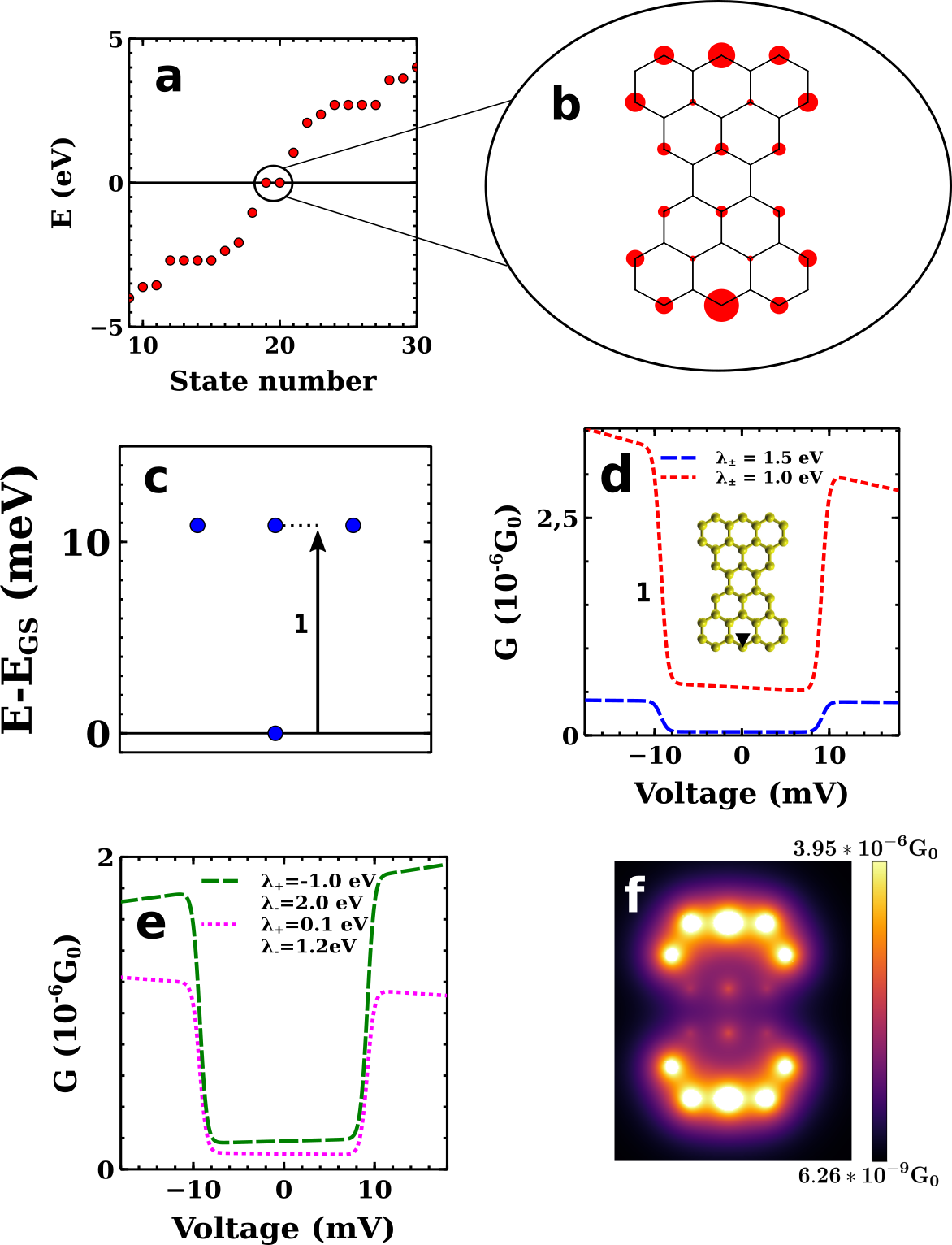
Figure 5: a) Tight-binding single-particle spectrum for the Clar’s goblet with $t=-2.7eV$ and $\delta t=-0.3t$ for the atom at the bottom edge, marked in the inset of panel (d), and b) is the corresponding wavefunction for the zero modes. c) The ground state and first excited triplet calculated with the Hubbard model for $U=|t|$ and CAS(4,4). The transition from the former to the latter is represented by the arrow and labeled by 1. d) dI/dV curve with $\lambda_{\pm}=1.0eV$ (red) and $\lambda_{\pm}=1.5eV$ (blue). The black triangle points the atom where the tip is coupled. e) dI/dV curve for different dominant channels. $V_{S}=t/100$, $V_{T}=V_{S}/5$, $T=3K$, $\epsilon_{C}=-5.7eV$, $\rho_{\eta\sigma}=10/t$ and $\mu_{S}=-5.4eV$. f) Map of the Clar’s goblet conductance when $V_{bias}=-15mV$.

Figure 6: a) Tight-binding single-particle spectrum for triangulene with $t=-2.7eV$ and $\delta t=-0.3t$ for the atom at the bottom edge marked in the inset of panel (d), and b) the corresponding wavefunction for the zero modes. c) The first 6 eigenstates calculated with the Hubbard model for $U=|t|$ and CAS(4,4). Transitions from the ground state to the 2 first singlet excited states are represented as arrows and labeled by 1 and 2. d) dI/dV curve. The two first transitions from the ground state to the singlet excited states are seen as two separated steps, the black triangle points the atom where the tip is coupled. $V_{S}=t/50$, $V_{T}=V_{S}/10$, $T=3K$, $\rho_{\eta\sigma}=10/t$ and $\epsilon_{C}=-5.7eV$. e) Conductance curve with different off-plane applied magnetic fields, a dip around 0 bias appears as a consequence of the Zeeman effect. f) Map of the triangulene conductance when $V_{bias}=-310mV$.

IV.3 Triangulene

We now consider the triangulene shown in figure (2a) with 22 carbon sites. This is known to be a diradical with $S=1$(inoue01, ). Unlike the bowtie and the rectangular nanographene, the triangulene considered here has a sublattice imbalance, with 10 atoms in one sublattice and 12 in the other. As a result, the single-particle spectra features two sublattice polarized in-gap zero modes(Palacios08, ; Lado15, ; Ortiz19, ), as shown in figure (6a). Their wavefunctions (figure 6b) can be chosen as eigenstates of the $C_{3}$ symmetry operator(Ortiz19, ). The molecular orbitals of these $C_{3}$ symmetric zero modes have the same modulus(Ortiz19, ), and therefore a maximal overlap, that enhances ferromagnetic exchange.

The sublattice imbalance $N_{A}-N_{B}=2$ implies(Lieb89, ; JFR07, ) that the ground state of the triangulene, described with the Hubbard model at half filling and first neighbour hopping, has $S=1$. The many-body spectra, calculated with the CAS(4,4) approximation has a $S=1$ ground state followed by two degenerate singlets and then one more singlet. The peculiar degeneracy of the lowest energy excitation is a consequence of the $C_{3}$ symmetry.

When we compute the conductance for this symmetric configuration, we obtain an extremely small height of the inelastic step at the energy of the lowest triplet-singlet excitation. We can gain some insight on the origin of this result in the case of CAS(2,2). In this case, it can be seen that the contribution to the cotunneling matrix elements of the coupling between the triangulene and the substrate is proportional to $\sum_{i}\phi_{z}(i)$. Interestingly, the zero modes of undistorted triangulene can be chosen to satisfy the identity $\sum_{i}\phi_{z}(i)=0$, which automatically gives a vanishing cotunneling conductance. A finite, but small, conductance is obtained in the CAS(4,4) approximation.

The cotunneling conductance is further increased if we break the $C_{3}$ symmetry, by assuming that the atom underneath the tip is pulled out of the surface, reducing its hopping with the first neighbours in the triangulene (see equation 15). Upon this approximation the resulting single-particle wavefunction (figure 6b) has a larger weight on the atom underneath the tip, and is no longer true that $\sum_{i}\phi_{z}(i)=0$.

The resulting many-body spectra for the distorted triangulene is shown in figure(6c). As a result of the distorsion, the excited states with $S=0$ are no longer forming a doublet, as obtained in the $C_{3}$ symmetric case(Ortiz19, ). The cotunneling conductance of the deformed triangulene, with $B_{z}=0T$, is shown in figure (6d). It has two steps, corresponding to the inelastic excitation of the triangulene $S=1$ ground state towards the deformation-split excited doublet with $S=0$.

Application of a magnetic field brings an effect specific of the $S=1$ ground state. Because of the Zeeman splitting, the state with magnetic moment parallel to the applied field becomes predominantly dominated at low temperature, and the others become depleted. This entails a reduction of the elastic cotunneling contribution that diminishes the zero bias conductance. In addition, a new finite bias inelastic step appears for $|e|V_{bias}=\pm g\mu_{B}|B_{z}|$. These two effects are shown in figure (6e). Observation of this feature would provide a conclusive confirmation of the $S>0$ nature of the ground state. We believe this effect has been observed by Li and coworkers(li2019, ), although they also observe a $S=1$ Kondo peak that can only be captured if we treat interaction with the substrate going beyond the second order perturbation theory discussed above(jacob16, ).

In figure (6f) we show the map for the dI/dV signal for $V_{bias}=-310mV$. As in the case of bowtie and rectangular nanoribbons, mapping the inelastic conductance provides an additional variable to probe the excitations and relate them to the zero modes, whose molecular orbitals are peaked at the edges.

V Discussion

V.1 Conditions for the observation of inelastic cotunneling steps

Cotunneling theory predicts the observation of cotunneling steps in every structure for which the inelastic excitation of the $N=N_{s}$ manifold is significantly smaller than the addition and substraction energy peaks. Whereas this type of excitations have now been reported in several structures(NachoNat, ; li2019, ; mishra19b, ) they are conspicuously missing in all triangulenes (pavlivcek2017, ; su19, ; mishra19, ) as well as in the rectangular ribbons(KimoucheNat2015, ; wang2016, ; Ruffieux16, ).

There are several factors that are known to reduce the visibility of cotunneling steps:

1. Thermal broadening(lambe68, ), approximately given by $5.4k_{B}T$. This could blur the inelastic steps of low energy excitations, such as the Zeeman split ground to ground transitions in the triangulene, or the singlet to triplet transitions of long rectangular ribbons for which exchange energy decays exponentially with size (Ortiz18, ).

2. Lock-in voltage. The resolution of the inelastic steps cannot be better than the lock-in voltage. Therefore, application of lock-in voltages larger than the inelastic excitations compromises their visibility.

3. Excitation lifetime effects. Inelastic tunneling spectroscopy is probing the spectral function of the collective excitations(JFR09, ). The poles of this spectral function are broadened by the inverse of their lifetimes. Kondo coupling to the substrate results in a broadening proportional to the energy of the excitation(delgado10, ; khajetoorians11, ).

4. Competition with sequential processes. The sequential tunneling is a resonant process, and therefore contributes much more strongly to the conductance. This could shadow inelastic steps whose energy is not sufficiently different from the sequential peak.

In order to address the lack of experimental observation of cotunneling steps in $S=1$, $S=3/2$ and $S=2$ triangulenes, that have been recently synthetized and probed with STM(su19, ; mishra19, ), we have computed their triplet-singlet splitting. For $U=|t|$ the excitation energies are $\Delta=260,192,146meV$ for $S=1$, $S=3/2$ and $S=2$, respectively. In figure (7c,d) of the AppendixA we show the linear dependence of these energies on $U$. Inspection of the experimentally observed values for the $V_{-}$ peaks show that the visibility of the negative bias step for $S=3/2$ might be compromised.

V.2 Symmetry and bias dependence

The cotunneling theory naturally yields curves that, in addition to the step-like features when the bias matches the excitation energies of the system, can have both a superimposed finite voltage dependence away from the inelastic steps and/or a very different height of the steps for positive and negative bias. We refer to these two features as bias dependence and asymmetry.

Bias dependence is a consequence of the fact that the matrix elements in equations (30,31), that determine the effective tip-surface tunneling amplitudes in the cotunneling Hamiltonian(28), feature the electrode-averaged addition energies in the denominators(DelgadoPRB2011, ). When the bias voltage is comparable with some of the addition energies, these denominators could cancel. The cotunneling theory is only valid far from these values. However, even when the bias is away from these addition energies, these denominators bring a voltage dependence that only disappears when bias voltage is sufficiently far.

The cause of the asymmetry of the height of the steps at positive and negative bias is quite different. The ultimate origin of the asymmetry is the fact that coupling of the nanographene to the tip and the substrate is not symmetric. Hand wavingly, the process by which an electron tunnels from tip to one carbon atom and then tunnels from any atom of the nanographene towards the substrate has a very different amplitude from the reverse process, by which an electron tunnels from surface to any atom in the nanographene and then it tunnels from one carbon atom to the tip.

Numerical evidence of these statements is presented in the figure (8) in AppendixB. Figure (8a) shows a symmetric $dI/dV$ cotunneling curve for a Hubbard trimer symmetrically coupled to both electrodes. Figure (8b) shows a mildly asymmetric conductance when the two electrodes are connected to only one atom in a non-equivalent configuration. Finally, an extremely asymmetric conductance is obtained when the coupling to the electrodes is very different (see figure 8c).

V.3 Kondo

As discussed above, the observation of zero bias peaks at low temperature in some nanographenes (NachoNat, ; Ezawa2009, ; li2019, ; mishra2020, ) provides a very strong evidence of the emergence of local moments in graphene and their quenching via Kondo interaction with the substrate. The Hamiltonian (28) is a generalized Anderson model that can in principle describe Kondo correlations if we compute current to higher order in the graphene-electrode interaction(jacob16, ). This will be the subject of future work.

VI Summary and outlook

We have revisited both sequential tunneling and cotunneling theories, often used to model transport in quantum dots(LossPRB2004, ) and molecules(gaudenzi17, ) , and discussed their application to study STM spectroscopy of nanographenes on surfaces. The main goal is to understand how the STM $dI/dV$ measurements can convey information about the existence of local moments in the $\pi$ electrons of nanographenes. We have discussed in detail the case of three classes of diradical nanographenes that have been recently studied experimentally: rectangular nanoribbons, bowtie and triangulenes.

An important take home message is that sequential transport leads to peak features in $dI/dV$ that relate to the addition and substraction energies of the nanographenes and provide thereby no direct information of the spin states. Sequential transport can be used to infer the addition energy of a given frontier orbital, a quantity that plays a role in the formation of local moments in nanographenes.

In contrast, cotunneling spectroscopy provides direct information of the energies of neutral excitation of nanographenes. These energies can provide direct evidence of the formation of local moments, if supplemented with magnetic field dependence experiments. Specifically, cotunneling spectroscopy could be in principle used to determine if the spin of the ground state is finite: for $S>0$ ground state, application of a magnetic field can result in a dip at zero bias. STM also permits us to map the inelastic signal as the STM tip scans the molecules laterally. As discussed above, the $dI/dV$ maps so obtained have a similar profile than zero modes that host the unpaired electrons that form the local moments, highlighting their interconnection.

Both theory and STM experiments probing open shell nanographenes indicate that emergent moments are governed by large energy scales. In the case of triangulenes, the $S=1$ ground state is separated from $S=0$ excitations by a gap of several hundreds of meV, although this has not been observed experimentally yet. The $S=0$ ground state of Clar’s goblet is separated by the $S=1$ excited state by 23 meV, which implies an inter-molecule exchange interaction of that magnitude(Ortiz19, ).

Advances in on-surface synthesis make it possible to assemble larger structures that combine open shell fragments with finite spin and large intermolecular exchange interactions and to explore strong coupling carbon based structures, with exchange interactions that can be both ferro and antiferromagnetic. Given both the small magnetic anisotropy of carbon based magnetism(Lado2014prl, ), as well as their low dimensionality (0D, 1D or at most 2D), this kind of artificial structures will provide an ideal platform to explore quantum magnetism, very much like the case of magnetic adatoms(choi19, ; khajetoorians19, ).

Future theory work should address a more realistic treatment of the nanographene-substrate interaction that is able to provide a theory of the linewidth of both sequential and cotunneling features, the observation of Kondo effect(NachoNat, ; li2019, ), the effect of substrate induced spin relaxation and decoherence(delgado17, ), and the renormalization of the excitation energies due to Kondo coupling to the substrate(oberg14, ). The interplay between local moments in nanographenes and proximity induced superconductivity(san15, ; Lado2DShiba, ) should also be a fertile arena to discover exotic new phases of matter.

Acknowledgments We acknowledge A. Pérez-Guardiola, G. Catarina, J. C. Sancho-García, M. Shantanu, O. Gröning, P. Ruffieux, R. Fasel, and J. I. Pascual for fruitful discussions. We acknowledge financial support from MINECO-Spain (Grant No. MAT2016-78625-C2) and from the Portuguese Fundação para a Ciência e a Tecnologia (FCT) for the projects P2020-PTDC/FIS-NAN/4662/2014, P2020-PTDC/FIS-NAN/3668/2014 and UTAPEXPL/NTec/0046/2017 projects. JFR acknowledges Generalitat Valenciana funding (Prometeo2017/139). R. O. acknowledge ACIF/2018/175 (Generalitat Valenciana and Fondo Social Europeo).

Appendix A Dependence of the excitation energies on $U$

In this Appendix we show the dependence on $U$ of the excitation energies in the $N=N_{s}$ manifold for the 3 classes of systems considered in the paper (nanoribbon, bowtie, triangulene). These enegies determine the bias voltage at which inelastic steps appear. The results are shown in figure (7). The different $U$ dependence is discussed in the main text. In the case of the bowtie we also compute the dependence of the excitation energy on the third neighbour hopping $t_{3}$ (see right panel of figure 7b).

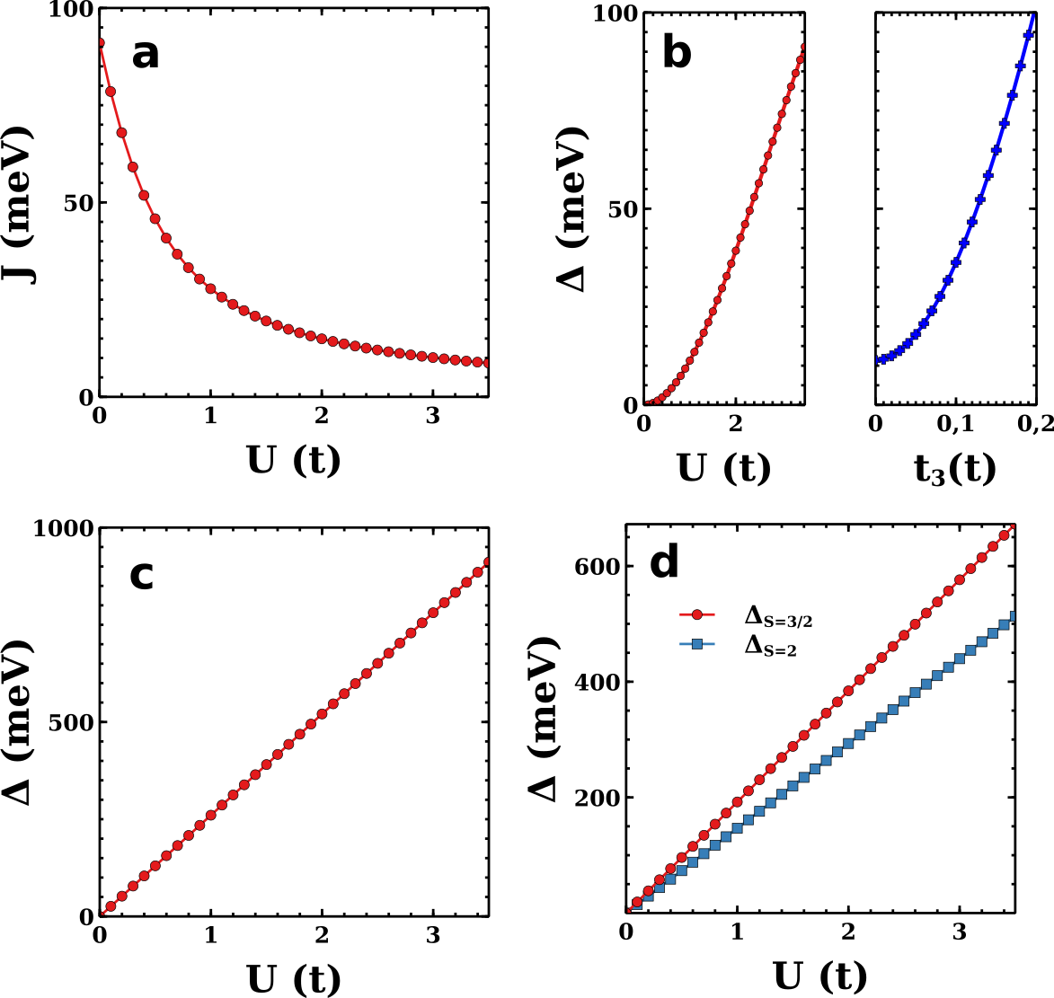
Figure 7: Splitting between the ground state and the first excited state for a) nanoribbon (CAS(2,2)), b) Clar’s goblet (CAS(4,4)), c) $S=1$ triangulene (CAS(2,2)) and d) $S=3/2$ (CAS(3,3)) and $S=2$ (CAS(4,4)) triangulenes, as function of $U$. $t=-2.7eV$ and $\epsilon_{C}=-5.7eV$. No hopping distortion was introduced here. For the Clar’s goblet, the dependence with third neighbour hopping is also displayed in panel right with constant $t_{2}=-0.071eV$ and $U=|t|$.

Appendix B Asymmetric inelastic steps height

As discussed in the main text, cotunneling spectra can feature different height in the inelastic steps for positive and negative bias. This is clearly seen in the rectangular ribbon, and less clear in the triangulene. The qualitative reason is discussed in the text and is ultimately due to the asymmetry of the coupling of the nanographene to tip and surface . A numerical validation of this statement is shown in figure (8).

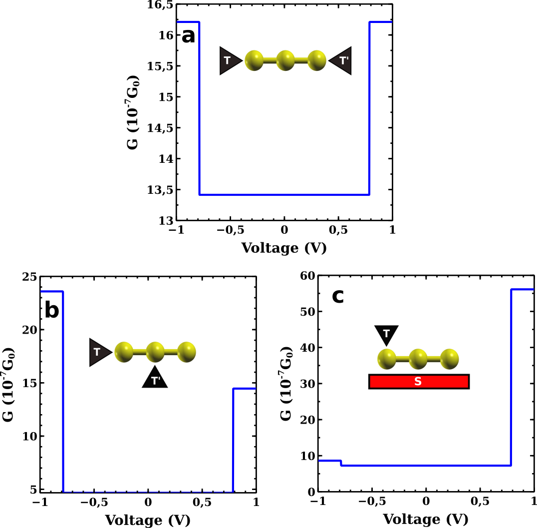
Figure 8: dI/dV curves for the Hubbard trimer when a) two tips are linked to the side atoms, b) one tip is linked to a side atom and a second tip to the center atom, and c) one electrode is a tip and the other is a surface. CAS(3,3), $E_{F}=0eV$, $t=-1eV$, $U=4|t|$, $Ed=-2.0eV$, $V_{S,T^{\prime}}=t/50$, $V_{T}=V_{S}/10$, $\rho_{\eta\sigma}=10/t$ and $T=1K$. Here both $\mu_{\eta}$ and $\mu_{\eta^{\prime}}$ are a function of bias, so the bias dependence is avoided for clarity. This calculation was performed without hopping distortion.

References

- (1) Nakada, K., Fujita, M., Dresselhaus, G. & Dresselhaus, M. S. Edge state in graphene ribbons: Nanometer size effect and edge shape dependence. Physical Review B 54, 17954 (1996).
- (2) Fujita, M., Wakabayashi, K., Nakada, K. & Kusakabe, K. Peculiar localized state at zigzag graphite edge. JPSJ 65, 1920–1923 (1996).
- (3) Ma, Y., Lehtinen, P., Foster, A. S. & Nieminen, R. M. Magnetic properties of vacancies in graphene and single-walled carbon nanotubes. New Journal of Physics 6, 68 (2004).
- (4) Vozmediano, M., López-Sancho, M., Stauber, T. & Guinea, F. Local defects and ferromagnetism in graphene layers. Physical Review B 72, 155121 (2005).
- (5) Son, Y.-W., Cohen, M. L. & Louie, S. G. Energy gaps in graphene nanoribbons. PRL 97, 216803 (2006).
- (6) Son, Y.-W., Cohen, M. L. & Louie, S. G. Half-metallic graphene nanoribbons. Nature 444, 347 (2006).
- (7) Yazyev, O. V. & Helm, L. Defect-induced magnetism in graphene. Physical Review B 75, 125408 (2007).
- (8) Fernández-Rossier, J. & Palacios, J. J. Magnetism in graphene nanoislands. PRL 99, 177204 (2007).
- (9) Uchoa, B., Kotov, V. N., Peres, N. M. R. & Castro Neto, A. H. Localized magnetic states in graphene. Phys. Rev. Lett. 101, 026805 (2008).
- (10) Kumazaki, H. & S. Hirashima, D. Nonmagnetic-defect-induced magnetism in graphene. JPSJ 76, 064713 (2007).
- (11) Brey, L., Fertig, H. A. & Das Sarma, S. Diluted graphene antiferromagnet. Phys. Rev. Lett. 99, 116802 (2007).
- (12) Palacios, J. J., Fernández-Rossier, J. & Brey, L. Vacancy-induced magnetism in graphene and graphene ribbons. Physical Review B 77, 195428 (2008).
- (13) Fernández-Rossier, J. Prediction of hidden multiferroic order in graphene zigzag ribbons. Physical Review B 77, 075430 (2008).
- (14) Ezawa, M. Metallic graphene nanodisks: Electronic and magnetic properties. Phys. Rev. B 76, 245415 (2007).
- (15) Pereira, V. M., Dos Santos, J. L. & Neto, A. C. Modeling disorder in graphene. Physical Review B 77, 115109 (2008).
- (16) Boukhvalov, D., Katsnelson, M. & Lichtenstein, A. Hydrogen on graphene: Electronic structure, total energy, structural distortions and magnetism from first-principles calculations. Physical Review B 77, 035427 (2008).
- (17) Yazyev, O. V. & Katsnelson, M. Magnetic correlations at graphene edges: basis for novel spintronics devices. Physical Review Letters 100, 047209 (2008).
- (18) Castro, E. V., López-Sancho, M. P. & Vozmediano, M. A. Pinning and switching of magnetic moments in bilayer graphene. New Journal of Physics 11, 095017 (2009).
- (19) Güçlü, A., Potasz, P., Voznyy, O., Korkusinski, M. & Hawrylak, P. Magnetism and correlations in fractionally filled degenerate shells of graphene quantum dots. Physical review letters 103, 246805 (2009).
- (20) Guo, G.-P. et al. Quantum computation with graphene nanoribbon. New Journal of Physics 11, 123005 (2009).
- (21) Jung, J., Pereg-Barnea, T. & MacDonald, A. H. Theory of interedge superexchange in zigzag edge magnetism. Physical review letters 102, 227205 (2009).
- (22) López-Sancho, M. P., de Juan, F. & Vozmediano, M. A. Magnetic moments in the presence of topological defects in graphene. Physical Review B 79, 075413 (2009).
- (23) Wang, W. L., Yazyev, O. V., Meng, S. & Kaxiras, E. Topological frustration in graphene nanoflakes: magnetic order and spin logic devices. Physical review letters 102, 157201 (2009).
- (24) Yazyev, O. V. Emergence of magnetism in graphene materials and nanostructures. Rep. Prog. Phys. 73, 056501 (2010).
- (25) Santos, E. J., Ayuela, A. & Sánchez-Portal, D. First-principles study of substitutional metal impurities in graphene: structural, electronic and magnetic properties. New Journal of Physics 12, 053012 (2010).
- (26) Soriano, D. et al. Magnetoresistance and magnetic ordering fingerprints in hydrogenated graphene. Physical review letters 107, 016602 (2011).
- (27) Culchac, F., Latgé, A. & Costa, A. Spin waves in zigzag graphene nanoribbons and the stability of edge ferromagnetism. New Journal of Physics 13, 033028 (2011).
- (28) Mizukami, W., Kurashige, Y. & Yanai, T. More electrons make a difference: emergence of many radicals on graphene nanoribbons studied by ab initio dmrg theory. Journal of chemical theory and computation 9, 401–407 (2012).
- (29) Akhukov, M. A., Fasolino, A., Gornostyrev, Y. N. & Katsnelson, M. I. Dangling bonds and magnetism of grain boundaries in graphene. Physical Review B 85, 115407 (2012).
- (30) Ij s, M. et al. Electronic states in finite graphene nanoribbons: Effect of charging and defects. Physical Review B 88, 075429 (2013).
- (31) Soriano, D. & Fernández-Rossier, J. Interplay between sublattice and spin symmetry breaking in graphene. Physical Review B 85, 195433 (2012).
- (32) Golor, M., Koop, C., Lang, T. C., Wessel, S. & Schmidt, M. J. Magnetic correlations in short and narrow graphene armchair nanoribbons. Physical review letters 111, 085504 (2013).
- (33) Golor, M., Lang, T. C. & Wessel, S. Quantum monte carlo studies of edge magnetism in chiral graphene nanoribbons. Physical Review B 87, 155441 (2013).
- (34) Lado, J. L. & Fernández-Rossier, J. Magnetic edge anisotropy in graphenelike honeycomb crystals. PRL 113, 027203 (2014).
- (35) Gargiulo, F. & Yazyev, O. V. Topological aspects of charge-carrier transmission across grain boundaries in graphene. Nano Lett. 14, 250–254 (2014).
- (36) Melle-Franco, M. Uthrene, a radically new molecule? Chemical Communications 51, 5387–5390 (2015).
- (37) Lado, J., García-Martínez, N. & Fernández-Rossier, J. Edge states in graphene-like systems. Synth. Met. 210, 56–67 (2015).
- (38) Phillips, M. & Mele, E. J. Zero modes on zero-angle grain boundaries in graphene. Physical Review B 91, 125404 (2015).
- (39) Lado, J. L. & Fernández-Rossier, J. Unconventional yu-shiba-rusinov states in hydrogenated graphene. 2D Mater. 3 (2016).
- (40) Weik, N., Schindler, J., Bera, S., Solomon, G. C. & Evers, F. Graphene with vacancies: Supernumerary zero modes. Physical Review B 94, 064204 (2016).
- (41) Das, A., Müller, T., Plasser, F. & Lischka, H. Polyradical character of triangular non-kekulé structures, zethrenes, p-quinodimethane-linked bisphenalenyl, and the clar goblet in comparison: An extended multireference study. J. Phys. Chem. A 120, 1625–1636 (2016).
- (42) López-Sancho, M. P. & Brey, L. Charged topological solitons in zigzag graphene nanoribbons. 2D Mater. 5 (2017).
- (43) Cao, T., Zhao, F. & Louie, S. G. Topological phases in graphene nanoribbons: Junction states, spin centers, and quantum spin chains. PRL 119, 076401 (2017).
- (44) García-Martínez, N. A., Lado, J. L., Jacob, D. & Fernández-Rossier, J. Anomalous magnetism in hydrogenated graphene. Physical Review B 96, 024403 (2017).
- (45) Melle-Franco, M. Graphene fragments: When 1+ 1 is odd. Nature nanotechnology 12, 292 (2017).
- (46) Ortiz, R., García-Martínez, N. A., Lado, J. L. & Fernández-Rossier, J. Electrical spin manipulation in graphene nanostructures. Physical Review B 97, 195425 (2018).
- (47) Ortiz, R. et al. Exchange rules for diradical -conjugated hydrocarbons. Nano Lett. 19, 5991–5997 (2019).
- (48) García-Martínez, N. & Fernández-Rossier, J. Designer fermion models in functionalized graphene bilayers. Phys. Rev. Research 1, 033173 (2019).
- (49) Morita, Y., Suzuki, S., Sato, K. & Takui, T. Synthetic organic spin chemistry for structurally well-defined open-shell graphene fragments. Nature chemistry 3, 197 (2011).
- (50) Lieb, E. H. Two theorems on the hubbard model. PRL 62, 1201–1204 (1989).
- (51) Inoue, J. et al. The first detection of a clar’s hydrocarbon, 2, 6, 10-tri-tert-butyltriangulene: a ground-state triplet of non-kekulé polynuclear benzenoid hydrocarbon. Journal of the American Chemical Society 123, 12702–12703 (2001).
- (52) Nair, R. et al. Dual origin of defect magnetism in graphene and its reversible switching by molecular doping. Nature communications 4, 2010 (2013).
- (53) Makarova, T. et al. Edge state magnetism in zigzag-interfaced graphene via spin susceptibility measurements. Scientific reports 5, 13382 (2015).
- (54) Lyon, T. J. et al. Probing electron spin resonance in monolayer graphene. Physical review letters 119, 066802 (2017).
- (55) Sepioni, M., Nair, R., Tsai, I.-L., Geim, A. & Grigorieva, I. Revealing common artifacts due to ferromagnetic inclusions in highly oriented pyrolytic graphite. EPL (Europhysics Letters) 97, 47001 (2012).
- (56) Özyilmaz, B., Jarillo-Herrero, P., Efetov, D. & Kim, P. Electronic transport in locally gated graphene nanoconstrictions. Applied Physics Letters 91, 192107 (2007).
- (57) Tao, C. et al. Spatially resolving edge states of chiral graphene nanoribbons. Nature Physics 7, 616 (2011).
- (58) Cai, J. et al. Atomically precise bottom-up fabrication of graphene nanoribbons. Nature 466, 470 (2010).
- (59) Kimouche, A. et al. Ultra-narrow metallic armchair graphene nanoribbons. Nat. Comm. 6 (2015).
- (60) Wang, S. et al. Giant edge state splitting at atomically precise graphene zigzag edges. Nat. Comm. 7 (2016).
- (61) Ruffieux, P. et al. On-surface synthesis of graphene nanoribbons with zigzag edge topology. Nature 531, 489–492 (2016).
- (62) Pavliček, N. et al. Synthesis and characterization of triangulene. Nat. Nanotechnol. 18, 308–311 (2017).
- (63) Su, J. et al. Atomically precise bottom-up synthesis of -extended [5] triangulene. Science advances 5, eaav7717 (2019).
- (64) Mishra, S. et al. Synthesis and characterization of -extended triangulene. Journal of the American Chemical Society (2019).
- (65) Rizzo, D. J. et al. Topological band engineering of graphene nanoribbons. Nature 560, 204–208 (2018).
- (66) Gröning, O. et al. Engineering of robust topological quantum phases in graphene nanoribbons. Nature 560, 209–213 (2018).
- (67) Bronner, C. et al. Hierarchical on-surface synthesis of graphene nanoribbon heterojunctions. ACS Nano 12, 2193–2200 (2018).
- (68) González-Herrero, H. et al. Atomic-scale control of graphene magnetism by using hydrogen atoms. Science 352, 437–441 (2016).
- (69) Heinrich, A. J., Gupta, J. A., Lutz, C. P. & Eigler, D. M. Single-atom spin-flip spectroscopy. Science 306, 466–469 (2004).
- (70) Hirjibehedin, C. et al. Large magnetic anisotropy of a single atomic spin embedded in a surface molecular network. Science 317, 1199 (2007).
- (71) Khajetoorians, A. A. et al. Itinerant nature of atom-magnetization excitation by tunneling electrons. Physical Review Letters 106, 037205 (2011).
- (72) Hirjibehedin, C. F., Lutz, C. P. & Heinrich, A. J. Spin coupling in engineered atomic structures. Science 312, 1021 (2006).
- (73) Spinelli, A., Bryant, B., Delgado, F., Fernández-Rossier, J. & Otte, A. F. Imaging of spin waves in atomically designed nanomagnets. Nature materials 13, 782 (2014).
- (74) Chen, X. et al. Probing superexchange interaction in molecular magnets by spin-flip spectroscopy and microsocpy. Phys. Rev. Lett. 101, 197208 (2008).
- (75) Tsukahara, N. et al. Adsorption-induced switching of magnetic anisotropy in a single iron(ii) phthalocyanine molecule on an oxidized cu(110) surface. Phys. Rev. Lett. 102, 167203 (2009).
- (76) Burgess, J. A. et al. Magnetic fingerprint of individual fe 4 molecular magnets under compression by a scanning tunnelling microscope. Nature communications 6, 8216 (2015).
- (77) Toskovic, R. et al. Atomic spin-chain realization of a model for quantum criticality. Nature Physics 12, 656 (2016).
- (78) Delgado, F. & Fernández-Rossier, J. Cotunneling theory of atomic spin inelastic electron tunneling spectroscopy. Physical Review B 84 (2011).
- (79) Fernández-Rossier, J. Theory of single-spin inelastic tunneling spectroscopy. Phys. Rev. Lett. 102, 256802 (2009).
- (80) Gauyacq, J.-P., Lorente, N. & Novaes, F. D. Excitation of local magnetic moments by tunneling electrons. Progress in surface science 87, 63–107 (2012).
- (81) Li, J. et al. Single spin localization and manipulation in graphene open-shell nanostructures. Nat. Comm. 10 (2019).
- (82) Li, J. et al. Atomic-scale engineering of magnetic graphene nanostructures. arXiv preprint arXiv:1912.08298 (2019).
- (83) Melle-Franco, M. Bow in awe to the new nanographene. Nat. Nanotechnol. (2019).
- (84) Mishra, S. et al. Topological frustration induces unconventional magnetism in a nanographene. Nature Nanotechnology 1–7 (2019).
- (85) Mishra, S. et al. Topological defect-induced magnetism in a nanographene. Journal of the American Chemical Society (2020).
- (86) Ervasti, M. M., Schulz, F., Liljeroth, P. & Harju, A. Single-and many-particle description of scanning tunneling spectroscopy. Journal of Electron Spectroscopy and Related Phenomena 219, 63–71 (2017).
- (87) Golovach, V. N. & Loss, D. Transport through a double quantum dot in the sequential tunneling and cotunneling regimes. Physical Review B 69 (2004).
- (88) Repp, J., Meyer, G., Stojkovic, S. M., Gourdon, A. & Joachim, C. Molecules on insulating films: Scanning-tunneling microscopy imaging of individual molecular orbitals. PRL 94 (2005).
- (89) De Franceschi, S. et al. Electron cotunneling in a semiconductor quantum dot. Physical review letters 86, 878 (2001).
- (90) Wong, H. S., Durkan, C. & Chandrasekhar, N. Tailoring the local interaction between graphene layers in graphite at the atomic scale and above using scanning tunneling microscopy. ACS Nano 3, 3455–3462 (2009).
- (91) Koch, M., Ample, F., Joachim, C. & Grill, L. Voltage-dependent conductance of a single graphene nanoribbon. Nat. Nanotechnol. 7, 713–717 (2012).
- (92) Xu, P. et al. Atomic control of strain in freestanding graphene. Physical Review B 85, 121406 (2012).
- (93) Xu, P. et al. Electronic transition from graphite to graphene via controlled movement of the top layer with scanning tunneling microscopy. Physical Review B 86, 085428 (2012).
- (94) Georgi, A. et al. Tuning the pseudospin polarization of graphene by a pseudomagnetic field. Nano Lett. 17, 2240–2245 (2017).
- (95) Sobczyk, S., Donarini, A. & Grifoni, M. Theory of stm junctions for conjugated molecules on thin insulating films. Physical Review B 85 (2012).
- (96) Gaudenzi, R., Misiorny, M., Burzurí, E., Wegewijs, M. R. & van der Zant, H. S. Transport mirages in single-molecule devices. The Journal of Chemical Physics 146, 092330 (2017).
- (97) Ezawa, M. Coulomb blockade in graphene nanodisks. Phys. Rev. B 77, 155411 (2008).
- (98) Jacob, D. & Kurth, S. Many-body spectral functions from steady state density functional theory. Nano letters 18, 2086–2090 (2018).
- (99) Ervasti, M. M., Schulz, F., Liljeroth, P. & Harju, A. Single- and many-particle description of scanning tunneling spectroscopy. J. Electron. Spectroscop. 219, 63–71 (2017).
- (100) Repp, J., Meyer, G., Paavilainen, S., Olsson, F. E. & Persson, M. Scanning tunneling spectroscopy of cl vacancies in nacl films: Strong electron-phonon coupling in double-barrier tunneling junctions. Phys. Rev. Lett. 95, 225503 (2005).
- (101) Anderson, P. W. New approach to the theory of superexchange interactions. Phys. Rev. 115, 2–13 (1959).
- (102) Clar, E. & Mackay, C. Circobiphenyl and the attempted synthesis of 1: 14, 3: 4, 7: 8, 10: 11-tetrabenzoperopyrene. Tetrahedron 28, 6041–6047 (1972).
- (103) Jacob, D. & Fernández-Rossier, J. Competition between quantum spin tunneling and kondo effect. The European Physical Journal B 89, 210 (2016).
- (104) Lambe, J. & Jaklevic, R. Molecular vibration spectra by inelastic electron tunneling. Physical Review 165, 821 (1968).
- (105) Delgado, F. & Fernández-Rossier, J. Spin dynamics of current-driven single magnetic adatoms and molecules. Physical Review B 82, 134414 (2010).
- (106) Ezawa, M. Quasiphase transition and many-spin kondo effects in a graphene nanodisk. Phys. Rev. B 79, 241407 (2009).
- (107) Choi, D.-J. et al. Colloquium: Atomic spin chains on surfaces. Reviews of Modern Physics 91, 041001 (2019).
- (108) Khajetoorians, A. A., Wegner, D., Otte, A. F. & Swart, I. Creating designer quantum states of matter atom-by-atom. Nature Reviews Physics 1–13 (2019).
- (109) Delgado, F. & Fernández-Rossier, J. Spin decoherence of magnetic atoms on surfaces. Progress in Surface Science 92, 40–82 (2017).
- (110) Oberg, J. C. et al. Control of single-spin magnetic anisotropy by exchange coupling. Nature nanotechnology 9, 64 (2014).
- (111) San-Jose, P., Lado, J. L., Aguado, R., Guinea, F. & Fernández-Rossier, J. Majorana zero modes in graphene. Physical Review X 5, 041042 (2015).