Rotation sensing with improved stability using point source atom interferometry

Abstract

Point source atom interferometry is a promising approach for implementing robust, high-sensitivity, rotation sensors using cold atoms. However, its scale factor, i.e., the ratio between the interferometer signal and the actual rotation rate, depends on the initial conditions of the atomic cloud, which may drift in time and result in bias instability, particularly in compact devices with short interrogation times. We present two methods to stabilize the scale factor, one relying on a model-based correction which exploits correlations between multiple features of the interferometer output and works on a single-shot basis, and the other a self-calibrating method where a known bias rotation is applied to every other measurement, requiring no prior knowledge of the underlying model but reducing the sensor bandwidth by a factor of two. We demonstrate both schemes experimentally with complete suppression of scale factor drifts, maintaining the original rotation sensitivity and allowing for bias-free operation over several hours.

I Introduction

Cold atom interferometers (Tino and Kasevich, 2014) have achieved in recent years record sensitivities in acceleration and rotation sensing. As acceleration-sensing instruments, their applications range from precision measurements for fundamental research (Weiss et al., 1993; Dimopoulos et al., 2007; Müller et al., 2010; Bouchendira et al., 2011; Rosi et al., 2014; Zhou et al., 2015; Barrett et al., 2016; Parker et al., 2018; Becker et al., 2018) to geophysical measurements with mobile atomic gravimeters (Bongs et al., 2019; Wu, 2009; Farah et al., 2014; Freier et al., 2016; Ménoret et al., 2018; Bidel et al., 2018; Wu et al., 2019; Bidel et al., ), demonstrating both high sensitivity and high stability operation. Atom interferometry gyroscopes (Barrett et al., 2014; Gustavson et al., 1997; Stockton et al., 2011; Dickerson et al., 2013; Savoie et al., 2018; Chen et al., 2019) are useful for field applications such as gyrocompassing (Gauguet et al., 2009; Sugarbaker et al., 2013) and inertial navigation on mobile platforms (Jekeli, 2005; Canuel et al., 2006; Rakholia et al., 2014). Similarly to atomic and optical clocks, atomic gyroscopes hold the promise of enhanced stability compared to their classical counterparts, due to their scale factor being defined in terms of fundamental physical constants. Previous demonstrations of atom interferometry gyroscopes (Durfee et al., 2006; Savoie et al., 2018) have reached sensitivity and stability which compare favorably with state-of-the-art optical gyroscopes (Lefevre, 2014; Battelier et al., 2016).

Point source interferometry (PSI) is an atom interferometry technique for rotation sensing based on detecting the spatial frequency of the interference pattern across an atomic cloud. Originally developed in a 10-meter atomic fountain (Dickerson et al., 2013), the technique has also been applied in a sensor with cm-scale physics package (Hoth et al., 2016). Compared to other atom interferometry rotation sensing techniques, PSI has the benefits of experimental simplicity and inherent suppression of accelerations and vibrations. As such, it is an especially promising technique for field and mobile applications. However, unlike ideal atomic sensors, the scale factor of PSI, defined as the ratio between the measured spatial frequency of the fringe pattern and the applied rotation rate, is sensitive to the initial and final size of the atomic cloud (Hoth et al., 2017). This dependency is amplified when the expansion ratio of the cloud is small, as in compact sensors with short expansion times. As a result, PSI is susceptible to bias instability due to drifts in its technical attributes (Chen et al., 2019), preventing it from realizing its full potential as an atomic sensor and limiting its usefulness in applications requiring high stability over long time scales.

In this work, we introduce two approaches to stabilizing scale-factor drifts in PSI sensors. The first approach utilizes additional information extracted from each PSI image, namely the interference fringe contrast and atomic cloud final size, in addition to the fringe spatial frequency. We experimentally verify the physical model which describes the correlation between these parameters and then employ it to correct the scale factor independently for every PSI image. The second approach relies on alternately applying a known bias rotation rate to the sensor, in addition to the unknown measured rotation. Analyzing pairs of measurements with and without the bias rotation enables self-calibration of the scale factor correction and determination of the unknown rotation. We implement both schemes experimentally and demonstrate their ability to recover uncorrelated $\tau^{-1/2}$ averaging performance of the rotation sensor. We achieve suppression of scale factor drifts up to a factor of ten without any loss in sensitivity and on time scales of up to $10^{4}\,\mathrm{sec}$, far surpassing previous results.

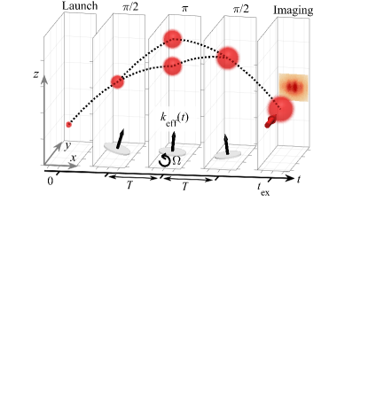
Figure 1: Schematic diagram of point source atom interferometry. The atomic cloud is launched upwards at $t=0$, interacts with a sequence of $\pi/2$-$\pi$-$\pi/2$ two-photon Raman pulses comprising the interferometer, and finally imaged at $t=t_{\textrm{ex}}$. The effective wave vector $\mathbf{k}_{\textrm{eff}}$ of the counter-propagating Raman beams is determined by a retro-reflecting mirror which can be tilted by a piezo stage to simulate rotations. Ballistic expansion of the cloud generates correlation between position and velocity of the atoms, giving rise to a spatial interference pattern from which the rotation rate is calculated.

II Point-source atom interferometry

PSI gyroscopes employs a Mach-Zehnder atom interferometer configuration (Kasevich and Chu, 1991). Three laser pulses, equally separated in time, interact with a freely-falling atomic cloud and act, in analogy to optical interferometry, as coherent beam splitters and mirrors. These operations are realized through counter-propagating laser beams which drive two-photon, Doppler-sensitive Raman transitions between different internal ground state levels and different momentum states of the atom (Kasevich et al., 1991). Beam splitter operations correspond to $\pi/2$-pulses which place the atom in a coherent superposition of two momentum states separated by $\hbar\mathbf{k}_{\textrm{eff}}$, where $\mathbf{k}_{\textrm{eff}}=\mathbf{k}_{1}-\mathbf{k}_{2}$ is the two-photon wave vector of the Raman interaction. Likewise, mirror operations correspond to $\pi$-pulses which change the momentum of each interferometer arm by $\pm\hbar\mathbf{k}_{\textrm{eff}}$. During the interferometer sequence, these pulses are utilized to coherently split, redirect, and recombine the atomic wavepackets in space (Fig. 1). The interferometer phase $\phi$ results from the different spatial trajectories of the two arms, and determines the relative population in the two internal states at the interferometer output. Through state-dependent detection of the atoms, this relative population and thus the phase can be measured.

In the Mach-Zehnder configuration considered here, the leading phase contributions are given by $\phi_{\mathbf{a}}=\left(\mathbf{k}_{\textrm{eff}}T^{2}\right)\cdot\mathbf{a}$ and $\phi_{\boldsymbol{\Omega}}=\left(2\mathbf{v}\times\mathbf{k}_{\textrm{eff}}T^{2}\right)\cdot\boldsymbol{\Omega}$, where $T$ is the time between each pair of pulses, $\mathbf{a}$ and $\boldsymbol{\Omega}$ are respectively the acceleration and rotation rate of the atoms relative to the interrogating Raman beams, and $\mathbf{v}$ is the mean velocity of each atom during the interferometer sequence. The acceleration phase $\phi_{\mathbf{a}}$ can be seen as resulting from the space-time area enclosed by the two interferometer arms, whereas the rotation phase $\phi_{\boldsymbol{\Omega}}$ results from the enclosed spatial area, in a Sagnac-like effect.

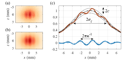
Figure 2: Spatial fringe pattern measured with PSI. (a) Raw fluorescence image from a single experiment. (b) Fit of the image to a two-dimensional Gaussian distribution with sinusoidal modulation. (c) Normalized, vertically integrated cross sections of the measured and fitted images (red dotted and solid lines, respectively). The Gaussian density distribution (dash-dotted line) of full width $2\sigma_{\textrm{f}}$ is modulated by a fringe pattern (blue) with spatial frequency $\kappa$ and contrast $c$. In this experiment, the initial cloud width was $2\sigma_{\textrm{i}}=0.98\,\mathrm{mm}$ (measured separately) with magnification of $\sigma_{\textrm{f}}/\sigma_{\textrm{i}}\sim 7.5$.

While $\phi_{\mathbf{a}}$ is uniform across the expanding atomic cloud, $\phi_{\boldsymbol{\Omega}}$ depends on the initial transverse velocity of each atom due to the cloud’s finite temperature. In the point-source limit, where the final cloud is much larger than its initial size, ballistic expansion of the cloud results in one-to-one correspondence between the atomic position and velocity. Thus, the velocity-dependent rotation phase is projected onto a spatial fringe pattern which may be directly imaged to facilitate a measurement of $\boldsymbol{\Omega}$ (Dickerson et al., 2013).

In our setup, the Raman beams are aligned vertically such that $\mathbf{k}_{\textrm{eff}}=k_{\textrm{eff}}\hat{\mathbf{z}}$, and the cloud is imaged in the $\hat{\mathbf{x}}\textrm{-}\hat{\mathbf{z}}$ plane, providing sensitivity to gravitational acceleration $-g\hat{\mathbf{z}}$ and to rotations around the $\mathbf{\hat{y}}$ axis. From here on, we will focus on the latter term only. For simplicity we denote $\Omega=\Omega_{y}$ and write the rotation phase as $\phi_{\Omega}=2k_{\textrm{eff}}\Omega v_{x}T^{2}$. In the point-source limit we have $x=v_{x}t_{\textrm{ex}}$, where $t_{\textrm{ex}}$ is the total expansion time of the cloud, and the rotation phase becomes $\phi_{\Omega}=\left(2k_{\textrm{eff}}\Omega T^{2}/t_{\textrm{ex}}\right)x$. The resulting atomic density has a profile of a modulated Gaussian distribution, as shown in Fig. 2, whose spatial frequency is given by $\kappa=\left(2k_{\textrm{eff}}T^{2}/t_{\textrm{ex}}\right)\Omega$. More generally we may write the spatial fringe frequency as $\kappa\left(\Omega\right)=F\Omega$ where $F$ is the scale factor, given in the point-source limit by $F_{\textrm{ps}}=2k_{\textrm{eff}}T^{2}/t_{\textrm{ex}}$ (Hoth et al., 2016).

In general, realization of a rotation-sensing atom interferometry requires separating the phase contributions of rotation and acceleration. In PSI this is achieved by exploiting the velocity-dependence of the rotation-sensitive phase $\phi_{\boldsymbol{\Omega}}$ to map it onto a spatially-varying interference pattern, separating rotation and acceleration into the spatial fringe frequency and phase, respectively (Chen et al., 2019). A different approach utilizes two atomic sources with opposite velocities, using either thermal (Gustavson et al., 1997) or cold atoms (Canuel et al., 2006), and performing identical Mach-Zehnder sequences on both. Here too, the velocity-dependence of $\phi_{\boldsymbol{\Omega}}$ results in the output phases of the two interferometers to be $\phi_{\mathbf{a}}\pm\phi_{\boldsymbol{\Omega}}$, allowing simple separation of the two contributions. Unlike PSI however, in these schemes $\phi_{\boldsymbol{\Omega}}$ is uniform for each of the two interferometers. Alternatively, a four-pulse “butterfly” interferometry sequence (Savoie et al., 2018) may be used, which inherently rejects the contribution of constant acceleration but remains sensitive to time-varying acceleration, such as vibration noise. In comparison to these two schemes, PSI offers a much simpler experimental configuration using only a single atomic source and a single interrogation optical beam, with suppression of both constant acceleration and vibrations.

III Experimental apparatus

In our apparatus (Yankelev et al., 2019; Avinadav et al., ), we load an ensemble of ${}^{87}\textrm{Rb}$ atoms from thermal background vapor in a magneto-optical trap (MOT) and cool them to $4\,\mathrm{\mu K}$. Through moving optical molasses, the atoms are launched vertically with velocities of up to $1.2\,\mathrm{m/s}$ while occupying all Zeeman states $m_{F}=0,\pm 1$ of the lower hyperfine level $F=1$. The interferometer pulses are realized by counter-propagating Raman beams with $\sigma^{+}-\sigma^{+}$ polarizations that drive two-photon transitions between the $m_{F}=0$ states of $F=1$ and $F=2$, with a bias magnetic field of about $300\,\mathrm{mG}$ to separate the magnetic Zeeman states.

Raman beams are realized by phase modulation at $\sim 6.834\,\mathrm{GHz}$ with an electro-optic modulator, with the carrier detuned $700\,\mathrm{MHz}$ red of the $F=2\rightarrow F^{\prime}=1$ transition, followed by a two-stage amplification to a total power of about $1\,\mathrm{W}$ in all sidebands. The Raman beam is collimated to $70\,\mathrm{mm}$ diameter using a Silicon Lightwave LB80 output collimator with $\lambda/10$ wavefront error. The resulting two-photon Rabi frequency is $35\,\mathrm{kHz}.$

The retro-reflecting mirror of the Raman beams is mounted on an accurate nanopositioning tip-tilt piezo stage (nPoint RXY3-410), which allows us to rotate the optical wavevector during the interferometer sequence and thereby mimic actual rotations. The stage has total dynamic range of $\pm 1.5\,\mathrm{mrad}$ in closed-loop operation, with $0.2\,\mathrm{\mu rad}$ position noise and a few milliseconds settling time.

Following the interferometer sequence, we use fluorescence excitation on the optical $F=2\rightarrow F^{\prime}=3$ cycling transition, employing all six MOT beams for minimal distortions, to capture an image of the atoms occupying the $F=2$ level. From launch to detection, the experimental sequence lasts in total up to $300\,\mathrm{ms}$. The shot-to-shot cycle time is $3\,\mathrm{s}$ due to technical limitations in communication bandwidth of the computer control system.

Images are taken on a PCO Pixelfly CCD camera, using a Fujinon-TV H6X12.5R zoom lens. We fit the image from each experiment to a Gaussian envelope function with sinusoidal modulation and extract $\kappa$, from which $\Omega$ is inferred (Fig. 2). We calibrate the imaging system by using velocity-selective Raman pulses and their well-known timing and momentum transfer, to select and image two narrow atomic ensembles at controllable distances.

IV Finite-size effects

IV.1 Theoretical model

For clouds of finite initial size, the resulting atomic density profile is a convolution of the initial density distribution with the ideal point-source fringe pattern, which is a spatial fringe superimposed on the unperturbed final density distribution. Mathematically, such convolution modifies both the wavelength and contrast of the fringe compared to the ideal point-source case. Hoth et al. derived analytically these effects assuming spherically-symmetric Gaussian initial and final density distributions (Hoth et al., 2017). In this case, both the spatial fringe frequency $\kappa$ and its contrast $c$ are reduced with respect to their values in the point-source limit. Defining the initial and final cloud widths as $\sigma_{\textrm{i}}$ and $\sigma_{\textrm{f}}$, respectively, the modified fringe properties were found to be

$$\kappa =F_{\textrm{ps}}\Omega\left(1-\sigma_{\textrm{i}}^{2}/\sigma_{\textrm{f}}^{2}\right),$$ (1)

$$c =c_{0}\exp\left[-\frac{1}{2}\frac{\kappa^{2}\sigma_{\textrm{i}}^{2}}{1-\sigma_{\textrm{i}}^{2}/\sigma_{\textrm{f}}^{2}}\right],$$ (2)

where $c_{0}$ is the interferometer contrast for $\Omega=0$.

In physical terms, imperfect correlation between the atoms’ position and velocity due to the finite-sized initial cloud results in averaging over atoms with different velocities at each measured position. For a Gaussian velocity distribution, the average velocity of atoms at each position is smaller than the expected value in the point-source limit, resulting in a reduction of the spatial fringe frequency. Similarly, the average over different velocities smears the interference fringes and reduces their contrast.

As a consequence of Eq. (1), the scale factor of the interferometer becomes $F=F_{\textrm{ps}}(1-\sigma_{\textrm{i}}^{2}/\sigma_{\textrm{f}}^{2})$. The dependency on $\sigma_{\textrm{i}}/\sigma_{\textrm{f}}$ leads to bias instability of the sensor when either $\sigma_{\textrm{i}}$ or $\sigma_{\textrm{f}}$ drift. Importantly, for a given relative drift in $\sigma_{\textrm{i}}$, the drift in the scale factor increases with the inverse magnification ratio $\sigma_{\textrm{i}}/\sigma_{\textrm{f}}$, emphasizing the susceptibility of compact sensors with small magnification to such drifts.

A larger magnification ratio can be achieved by decreasing $\sigma_{\textrm{i}}$ using, e.g., tight dipole traps, which adds experimental complexity and may impact the atom number; or by increasing $\sigma_{\textrm{f}}$ through longer expansion times or higher cloud temperatures, in either case requiring larger atom optics and detection beams. However, even when operating at a large magnification ratio such as $\sigma_{\textrm{f}}/\sigma_{\textrm{i}}=50$, the scale factor is modified by $400\,\mathrm{ppm}$ and small drifts in the initial cloud size on the order of a few percent would result in changes of tens parts per million to the scale factor. In comparison, optical gyroscopes achieve scale factor stability on the order of $1\,\mathrm{ppm}$ (Lefèvre, 2014).

IV.2 Experimental verification

We verify the model predictions by performing measurements with different values of $\sigma_{\textrm{i}}$, obtained through different repump intensities at the final optical molasses stage, and with different values $\sigma_{\textrm{f}}$, obtained through different launch velocities and thus different expansion times. $\sigma_{\textrm{i}}$ was measured in independent experiments by imaging the cloud immediately after launch. For standard operation of the optical molasses, the value of $\sigma_{\textrm{i}}$ is about $0.5\,\mathrm{mm}$, and we can increase it up to about $0.8\,\mathrm{mm}$ before suffering significant loss of atoms. As Fig. 3 shows, we find good agreement with the functionals in Eqs. (1) and (2) for a range of magnification ratios $\sigma_{\textrm{f}}/\sigma_{\textrm{i}}$ between $3.5$ and $9$, corresponding to changes of 5% in scale factor. The fact that the scale factor $F$ at $\sigma_{\textrm{i}}/\sigma_{\textrm{f}}\rightarrow 0$ differs from $F_{\textrm{ps}}$ by 3.5% can be attributed to imaging distortions and to residual calibration errors of the imaging system and of the piezo stage driving the mirror rotations. The fitted slope for the scale-factor dependence on $\sigma_{\textrm{i}}^{2}/\sigma_{\textrm{f}}^{2}$, as well as the scaling of the exponential decrease of the contrast, slightly differ from the theoretical model either due to estimation errors in $\sigma_{\textrm{i}}$ and $\sigma_{\textrm{f}}$ or due to non-Gaussian density distributions.

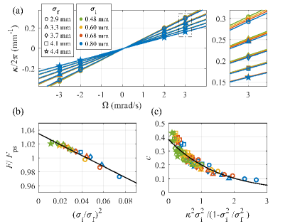
Figure 3: Effect of initial cloud size $\sigma_{\textrm{i}}$ and final cloud size $\sigma_{\textrm{f}}$ on PSI scale factor and contrast. (a) Measured spatial fringe frequency $\kappa$ as a function of $\Omega$ for different values of $\sigma_{\textrm{i}}$ and $\sigma_{\textrm{f}}$. Solid lines are linear fits, with slopes representing the scale factors. Different values of $\sigma_{\textrm{f}}$ correspond to launch velocities $0.6\textrm{-}1.2\,\mathrm{m/s}$, with $t_{\textrm{ex}}$ between $133\textrm{-}252\,\mathrm{ms}$. In all cases $T=52\,\mathrm{ms}$. (b) Measured scale factor for different values of $\sigma_{\textrm{i}}$ and $\sigma_{\textrm{f}}$. Solid line is a linear fit with slope $-0.79(4)$, deviating from the predicted value $-1$. (c) Measured fringe contrast for different values of $\sigma_{\textrm{i}}$ and $\sigma_{\textrm{f}}$. Solid line is an exponential fit to $c=c_{0}\exp\left[-\alpha\kappa^{2}\sigma_{\textrm{i}}^{2}/\left(1-\sigma_{\textrm{i}}^{2}/\sigma_{\textrm{f}}^{2}\right)\right]$ with $\alpha=0.65(3)$, deviating from the model prediction $\alpha=0.5$.

V Contrast-based stabilization

V.1 Model description

The first method we present for correcting scale factor instability exploits the correlation between $\Omega$ and $\left(\kappa,c,\sigma_{\textrm{f}}\right)$ which are extracted from each PSI image. We obtain the relation $\Omega\left(\kappa,c,\sigma_{\textrm{f}}\right)$ by eliminating $\sigma_{\textrm{i}}$ from Eqs. (1) and (2). To capture the aforementioned deviations from the model, we add a single parameter $\beta$ and replace $\sigma_{\textrm{f}}\rightarrow\sigma_{\textrm{f}}/\beta$. The resulting expression for $\Omega$ is then

$$\Omega=\frac{\kappa}{F_{\textrm{ps}}}\left[1-2\left(\frac{\beta}{\kappa\sigma_{\textrm{f}}}\right)^{2}\ln\frac{c}{c_{0}}\right].$$ (3)

As demonstrated below, we verify that this formulation, based on one physical parameter $c_{0}$ and one correction parameter $\beta$, provides an excellent description of the measured data. Importantly, it allows us to calculate $\Omega$ using only the parameters $\kappa$, $c$ and $\sigma_{\textrm{f}}$ measured in every single PSI image, enabling analysis on a single-shot basis without any reduction in temporal bandwidth.

V.2 Parameter calibration

To calibrate $c_{0}$ and $\beta$ in Eq. (3), we perform measurements at a constant rotation rate and periodically vary $\sigma_{\textrm{i}}$ by changing the repump beam intensity during the moving optical molasses. This results in changes to $c$, $\sigma_{\textrm{f}}$, and $\kappa$, as shown in Fig. 4(a). Inverting Eq. (3) and setting $\Omega=\Omega_{\textrm{calib}}$, we obtain an expression for $\kappa$ in this calibration measurement,

$$\kappa=\frac{1}{2}F_{\textrm{ps}}\Omega_{\textrm{calib}}\left[1+\sqrt{1+\frac{8\ln\left(c/c_{0}\right)}{\left(F_{\textrm{ps}}\Omega_{\textrm{calib}}\sigma_{\textrm{f}}/\beta\right)^{2}}}\right].$$ (4)

The measured data points are fitted to this surface equation, as shown in Fig. 4(b), where $c_{0}$, $\beta$, and $\Omega_{\textrm{calib}}$ are the fit parameters, the latter being an auxiliary parameter not used in any subsequent analysis.

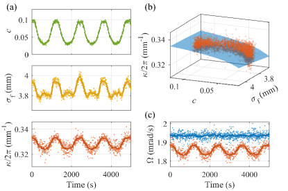
Figure 4: Calibration of contrast-based scale-factor stabilization. (a) Top to bottom: measured contrast, final cloud size, and spatial fringe frequency for an applied rotation rate of $2\,\mathrm{mrad/s}$, as $\sigma_{\textrm{i}}$ is varied periodically in the range $0.5-0.8\,\mathrm{mm}$. Each data point represents a single PSI image. In these and following experiments, $T=80\,\mathrm{ms}$ and $t_{\textrm{ex}}=185\,\mathrm{ms}$. (b) Parametric plot of $\kappa\left(c,\sigma_{\textrm{f}}\right)$. Dots are data points, surface is a fit to Eq. (4) with $c_{0}=0.43(8)$ and $\beta=0.80(1)$. The fit describes the data points well, with residuals of $\kappa$ from the fit surface showing no correlation to $c$ or $\sigma_{\textrm{f}}$ and characterized by standard deviation $\left(2\pi\right)2.49\times 10^{-3}\,\mathrm{mm^{-1}}$, consistent with a moving standard deviation $\left(2\pi\right)2.55\times 10^{-3}\,\mathrm{mm^{-1}}$ of the raw $\kappa$ measurements. (c) Rotation rate calculated with the uncorrected scale-factor $F_{\textrm{ps}}$ (red), compared to corrected rotation rate (blue), which employs Eq. (3) with the calibrated parameters, showing excellent rejection of scale-factor drifts. Solid lines in (a),(c) are 30-samples moving averages.

With calibrated $c_{0}$ and $\beta$ at hand, we now use Eq. (3) to correct the inferred rotation rate in this calibration run. This exercise is shown in Fig. 4(c), and indeed we find that the drifts are removed and a stable rotation measurement is obtained. We emphasize that the analysis does not use any assumption or prior knowledge on $\sigma_{\textrm{i}}$ or on its temporal variations, and in fact the only prerequisite is that the range of $\sigma_{\textrm{i}}$ scanned during the calibration process is large enough to adequately calibrate the model parameters.

While this correction is aimed to improve the measurement stability under variations of $\sigma_{\textrm{i}}$, the measurement accuracy is enhanced as well. As Eq. (3) captures also the systematic bias due to the finite magnification ratio, as described by Eq. (1), applying this correction suppresses the systematic bias. Indeed, we find the post-correction estimated rotation rate [Fig. 4(c)] to be $1.936(6)\,\mathrm{mrad/s}$, in agreement with the expected value $1.9387\,\mathrm{mrad/s}$ which consists of the applied mirror rotation rate of $2\,\mathrm{mrad/s}$ and the projection of Earth’s rotation on the measurement axis, which was due north, at our latitude of $32.7940^{\circ}\,\mathrm{N}$. In contrast, the mean estimated rotation rate using the point-source scale factor is $1.857\,\mathrm{mrad/s}$, differing significantly from the true value.

Nevertheless, it is possible that some residual bias still exists after applying Eq. (3). However, it would be inseparable from other possible sources of systematic bias in the PSI measurement due to, e.g., effect of wavefront aberrations (Gauguet et al., 2009; Schkolnik et al., 2015; Karcher et al., 2018) or imaging distortions. Calibration error of the piezo stage and inaccurate estimation of the measurement axis north alignment will contribute to an apparent bias as well. For this reason $\Omega_{\textrm{calib}}$ is treated as a fit parameter when using Eq. (4), rather than being simply taken as the input rotation rate. The overall bias may be corrected by calibrating the PSI sensor, for example using a precision rotary stage.

V.3 Demonstration of correction performance

We demonstrate the implementation of this stabilization method in two separate measurement runs, as presented in Fig. 5, representing realistic operating scenarios where the rotation rate varies in time. We artificially generate scale-factor drifts by varying the optical molasses parameters which affect the initial and final cloud distributions, both in periodic fashion and in random-walk-like behavior. While the rotation rate and initial conditions change smoothly in time, this information is not used in the analysis as all corrections are on a single-shot basis. The interferometer parameters are $T=80\,\mathrm{ms}$ and $t_{\textrm{ex}}=185\,\mathrm{ms}$, as in the calibration run.

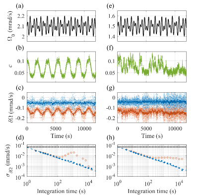
Figure 5: Demonstration of contrast-based scale-factor stabilization. (a) Time series of the input rotation rate $\Omega_{0}$, oscillating around $2.1\,\mathrm{mrad/s}$. (b) Measured fringe contrast shows variations due to applied periodic changes to $\sigma_{\textrm{i}}$. (c) Residuals of the estimated rotation rate $\Omega-\Omega_{0}$, with (blue) and without (red) scale-factor correction using Eq. (3). Solid lines are 30-samples moving averages. The full data spans $3\times 10^{4}\,\mathrm{sec}$. (d) Allan deviation of the residuals, with and without scale factor correction. Dashed line is a fit to $\tau^{-1/2}$. Dotted line indicates Earth rotation rate at our lab location. (e-h) Same as (a-d), with $\Omega_{0}$ oscillating around $1.5\,\mathrm{mrad/s}$ and random-walk variations in $\sigma_{\textrm{i}}$ in the range $0.5-0.8\,\mathrm{mm}$. The observed sensitivities are $28\,\mathrm{\mu rad/s}$, $32\,\mathrm{\mu rad/s}$ per shot in panels (d), (h), respectively, differing slightly due to changing experimental conditions, such as total atom number.

Using Eq. (3) and the previously calibrated values for $c_{0}$ and $\beta$, we obtain suppression of sensor drifts by a factor of ten in both examples [Fig. 5(d),(h)], limited only by the magnitude of the drifts we introduced. The scheme allows complete recovery of $\tau^{-1/2}$ averaging performance at time scales up to $10^{4}$ seconds, affirming that it does not introduce new bias instabilities of its own. The second example, where $\Omega$ varies around a mean value smaller than $\Omega_{\textrm{calib}}$, and the model measurements shown in Fig. 3 with larger values of $\Omega$, demonstrate that the technique is robust and does not require multiple calibration runs with different values of $\Omega_{\textrm{calib}}$. Our measurements reach a stability of $0.5\,\mathrm{\mu rad/s}$, providing a upper bound for the scale-factor stability of $2.5\times 10^{-4}$. Under the applied variation of $\pm 18\%$ in $\sigma_{\textrm{i}}$ , reaching such stability without any correction scheme would require operating the PSI sensor at a magnification ratio of at least $40$.

Finally, we note that it is possible in principle to apply a correction similar to that described in this section by utilizing Eq. (1) and directly measuring $\sigma_{\textrm{i}}$. This may be done either in separate experimental shots, at the expense of reduced bandwidth and sensitivity per $\sqrt{\textrm{Hz}}$ and under the constraint that $\sigma_{\textrm{i}}$ changes little between shots, or through non-destructive imaging of the cloud during the final moving molasses stage. The latter is challenging as it requires short exposure time to avoid motion blur of the small, moving cloud. In addition to these constraints, as Fig. 3(b) demonstrates, Eq. (1) requires an additional scaling parameter to fit the measured data, likely due to the non-Gaussian shape of the initial cloud. Thus this approach of directly measuring $\sigma_{\textrm{i}}$ does not eliminate the need for calibration parameters.

VI Self-calibrating stabilization

VI.1 Principles and demonstration

Our second method for scale-factor stabilization utilizes the piezo rotation stage to apply a known rotation $\Omega_{\textrm{bias}}$ at alternating measurements, in addition to the unknown rotation $\Omega$ which we wish to measure. Denoting the scale factor in these measurements as $F$, the spatial fringe frequencies of two consecutive measurements are given by $\kappa_{1}=F\Omega$ and $\kappa_{2}=F\left(\Omega+\Omega_{\textrm{bias}}\right)$. These equations may be inverted to yield

$$\Omega =\Omega_{\textrm{bias}}\frac{\kappa_{1}}{\kappa_{2}-\kappa_{1}},$$ (5)

$$F =\frac{1}{\Omega_{\textrm{bias}}}\left(\kappa_{2}-\kappa_{1}\right),$$ (6)

allowing us to extract both $\Omega$ and $F$ from each pair of measurements $\kappa_{1}$ and $\kappa_{2}$. This self-calibrating method requires no prior knowledge or assumption of a model describing the relationship between $F$ and other system parameters. The signs of $\kappa_{1},\kappa_{2}$ are not directly available from the PSI images but rather assumed to be known, for example from an auxiliary rotation sensor, as in all existing schemes of PSI.

An experimental demonstration of the self-calibration method is shown in Fig. 6, with both the measured rotation $\Omega$ and the scale factor changing in time. Again we find perfect suppression of scale factor drifts and recovery of $\tau^{-1/2}$ noise behavior. Compared to the previously described contrast-based stabilization, this method reduces the effective bandwidth by a factor of two due to the pairwise analysis but has the advantages of being model-independent and not requiring any initial calibration measurements. We note that despite the reduction in bandwidth, information is not lost when analyzing pairs of measurements and thus the rotation sensitivity per $\sqrt{\textrm{Hz}}$ is maintained, as evident in Fig. 6(e).

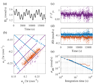
Figure 6: Demonstration of scale-factor stabilization by self-calibration. (a) Time series of the input rotation rate $\Omega_{0}$. (b) Measured $\kappa_{2}$ and $\kappa_{1}$, each dot corresponding to a pair of experiments with and without $\Omega_{\textrm{bias}}=-2.6\,\mathrm{mrad/s}$. Also shown are contour lines of the estimated rotation rate (blue) and scale factor correction relative to $F_{\textrm{ps}}$ (purple) based on Eqs. (5-6). (c) Estimated scale factor correction from each pair of measurements, showing random-walk variations due to applied changes to $\sigma_{\textrm{i}}$ in the range $0.5-0.8\,\mathrm{mm}$. (d) Residuals of the estimated rotation rate $\Omega-\Omega_{0}$, using the nominal scale factor $F=F_{\textrm{ps}}$ (red) and the corrected scale factor (blue). Solid lines in (c),(d) are 30-samples moving averages. (e) Allan deviation of the residuals, with and without scale factor correction. Dashed line is a fit to $\tau^{-1/2}$ with sensitivity $32\,\mathrm{\mu rad/s}$ per shot.

This correction scheme relies on an accurate piezo stage for adding a known bias rotation, as errors in $\Omega_{\textrm{bias}}$ enter directly into the estimation of $\Omega$ itself. Therefore the stage is required to have similar resolution as the PSI measurement so as not to degrade its sensitivity, and long-term stability to enable scale-factor corrections at long times. As our results show, these conditions are fulfilled in our apparatus. Indeed, such a stage with adequate performance is likely to be necessary anyway in an operational rotation sensor, for purposes such as calibration and dynamic range compensation.

VI.2 Generalization to time-varying scenarios

The analysis above assumed that $\Omega$ and $F$ are constant in both measurements. We now turn to the more general case where these quantities may change between shots. We define $\Omega_{1}=\Omega+\delta\Omega$, $\Omega_{2}=\Omega-\delta\Omega+\Omega_{\textrm{bias}}$, and $F_{1,2}=F_{0}+\delta F_{\textrm{comm}}\pm\delta F_{\textrm{diff}}$, such that the measured spatial fringe frequencies are $\kappa_{1,2}=F_{1,2}\Omega_{1,2}$. Here $\delta\Omega$ represents shot-to-shot variation in $\Omega$, $F_{0}$ is the nominal scale-factor, and $\delta F_{\textrm{comm}}$ and $\delta F_{\textrm{diff}}$ are scale-factor errors common and different, respectively, in both measurements. $\Omega_{\textrm{bias}}$ as before is the known rotation which is added in the second measurement. Using Eq. (5) and to leading order in $\delta\Omega/\Omega$ and $\delta F/F$, we find that the estimated rotation rate is

$$\frac{\Omega_{\textrm{est}}}{\Omega} \approx 1+\left(2+\frac{2\Omega}{\Omega_{\textrm{bias}}}\right)\frac{\delta F_{\textrm{diff}}}{F_{0}}+\left(1+\frac{2\Omega}{\Omega_{\textrm{bias}}}\right)\frac{\delta\Omega}{\Omega}$$ (7)

To eliminate the $\delta\Omega$-related term in Eq. (7), we set $\Omega_{\textrm{bias}}=-2\left(\kappa_{1}/F_{0}\right)$, where $\kappa_{1}/F_{0}$ corresponds to an estimate of $\Omega_{1}$ based on the first measurement and assuming the nominal scale-factor. With this choice of $\Omega_{\textrm{bias}}$, we have to leading order $\Omega_{\textrm{est}}\approx\Omega\left(1+\delta F_{\textrm{diff}}/F_{0}\right)$, such that the estimated rotation rate corresponds to the average $\Omega$ of the two measurements.

Regardless of the exact choice of $\Omega_{\textrm{bias}}$, we find that even in this case of varying-rotation rate and scale-factor, the result is insensitive to errors in the scale-factor which are common to both measurements and remains sensitive only to non-common scale-factor errors $\delta F_{\textrm{diff}}$. In contrast, the “naive” measurement approach, with $\Omega_{\textrm{bias}}=0$ and estimating $\Omega$ as the average $\frac{1}{2}\left(\kappa_{1}+\kappa_{2}\right)/F_{0}$, leads to $\Omega_{\textrm{naive}}\approx\Omega\left(1+\delta F_{\textrm{comm}}/F_{0}\right)$. It is then the non-common scale-factor error which cancels to leading order, and the common error remains.

In most scenarios, $\delta F_{\textrm{comm}}\gg\delta F_{\textrm{diff}}$ i.e., the scale-factor is expected to change slowly with respect to the time scale of two measurements, and thus our self-calibrating method cancels the more dominant source of error. Additionally, more advanced estimation protocols such as a Kalman filter (Kalman, 1960; Cheiney et al., 2018) could be used to track rapidly varying rotation signals while estimating the slowly-varying scale factor from multiple measurement pairs.

VII Conclusion

We have presented two complementary approaches for improving the stability of rotation measurements using point source atom interferometry, suppressing scale factor drifts which arise due to changes in the atomic cloud parameters. We demonstrated the two schemes experimentally with complete suppression of scale factor drifts. We showed that they maintain the sensor sensitivity and do not introduce any drifts on their own. We achieved scale-factor stability on time scales up to $10^{4}\,\mathrm{sec}$, representing orders of magnitude improvement in stability time compared to previous works. We reach rotation rate stability of $0.5\,\mathrm{\mu rad/s}$.

The first approach utilizes the inherent correlations between different parameters in PSI images, namely the contrast, spatial frequency and final size of the fringe pattern, for estimating the scale factor from a single image and correct for drifts. The underlying model which describes these correlations is based on the physics of the sensor, rather than on an empirical correlation, as we verify by independent measurements. This method is based on information which is already available in standard PSI measurements and maintains the original bandwidth of the sensor, however preliminary calibration of two model parameters is necessary. The possibility of using a continuous estimation protocol such as Kalman or particle filtering (Moral, 1997), to replace the initial calibration as well as to allow temporal variations of these parameters, may also be explored.

The second approach relies on sequential measurements with an added bias rotation to directly estimate the scale factor from each pair of measurements. This approach is self-calibrating and completely model-independent, but it depends on the stability of the piezo mirror stage generating the bias rotation and reduces the sensor bandwidth.

While the experiments described here focus on side-imaging PSI which allows single-axis rotation sensing, the two schemes we developed are fully compatible under the same conditions with dual-axis sensors using top- or bottom- imaging of the cloud.

The stabilization techniques we developed are particularly important in compact PSI sensors, which are an attractive alternative for constructing simple, mobile device with high sensitivity to rotations. Our schemes address a significant challenge of such PSI sensors, namely high susceptibility to scale factor drifts due to the low magnification ratio of the atomic cloud. The results may pave the way for realizing high-performance, compact PSI devices for demanding applications that require long-time stability, such as gyrocompasses for north finding applications, gyroscopes for line-of-sight stabilization, or inertial measurement units for navigation systems.

References

- Tino and Kasevich (2014) G. M. Tino and M. A. Kasevich, eds., Atom Interferometry, in Proceedings of the International School of Physics "Enrico Fermi," Course CLXXXVIII (Societa Italiana di Fisica and IOS Press, 2014).
- Weiss et al. (1993) D. S. Weiss, B. C. Young, and S. Chu, “Precision measurement of the photon recoil of an atom using atomic interferometry,” Physical Review Letters 70 (1993), 10.1103/physrevlett.70.2706.
- Dimopoulos et al. (2007) S. Dimopoulos, P. W. Graham, J. M. Hogan, and M. A. Kasevich, “Testing general relativity with atom interferometry,” Physical Review Letters 98 (2007), 10.1103/physrevlett.98.111102.
- Müller et al. (2010) H. Müller, A. Peters, and S. Chu, “A precision measurement of the gravitational redshift by the interference of matter waves,” Nature 463 (2010), 10.1038/nature08776.
- Bouchendira et al. (2011) R. Bouchendira, P. Cladé, S. Guellati-Khélifa, F. Nez, and F. Biraben, “New determination of the fine structure constant and test of the quantum electrodynamics,” Physical Review Letters 106 (2011), 10.1103/physrevlett.106.080801.
- Rosi et al. (2014) G. Rosi, F. Sorrentino, L. Cacciapuoti, M. Prevedelli, and G. M. Tino, “Precision measurement of the newtonian gravitational constant using cold atoms,” Nature 510 (2014), 10.1038/nature13433.
- Zhou et al. (2015) L. Zhou, S. Long, B. Tang, X. Chen, F. Gao, W. Peng, W. Duan, J. Zhong, Z. Xiong, J. Wang, Y. Zhang, and M. Zhan, “Test of equivalence principle at 10-8level by a dual-species double-diffraction raman atom interferometer,” Physical Review Letters 115 (2015), 10.1103/physrevlett.115.013004.
- Barrett et al. (2016) Brynle Barrett, Laura Antoni-Micollier, Laure Chichet, Baptiste Battelier, Thomas Lévèque, Arnaud Landragin, and Philippe Bouyer, “Dual matter-wave inertial sensors in weightlessness,” Nature Communications 7 (2016), 10.1038/ncomms13786.
- Parker et al. (2018) Richard H. Parker, Chenghui Yu, Weicheng Zhong, Brian Estey, and Holger Müller, “Measurement of the fine-structure constant as a test of the standard model,” Science 360 (2018), 10.1126/science.aap7706.
- Becker et al. (2018) Dennis Becker, Maike D. Lachmann, Stephan T. Seidel, Holger Ahlers, Aline N. Dinkelaker, Jens Grosse, Ortwin Hellmig, Hauke Müntinga, Vladimir Schkolnik, Thijs Wendrich, André Wenzlawski, Benjamin Weps, Robin Corgier, Tobias Franz, Naceur Gaaloul, Waldemar Herr, Daniel Lüdtke, Manuel Popp, Sirine Amri, Hannes Duncker, Maik Erbe, Anja Kohfeldt, André Kubelka-Lange, Claus Braxmaier, Eric Charron, Wolfgang Ertmer, Markus Krutzik, Claus Lämmerzahl, Achim Peters, Wolfgang P. Schleich, Klaus Sengstock, Reinhold Walser, Andreas Wicht, Patrick Windpassinger, and Ernst M. Rasel, “Space-borne bose-einstein condensation for precision interferometry,” Nature 562 (2018), 10.1038/s41586-018-0605-1.
- Bongs et al. (2019) Kai Bongs, Michael Holynski, Jamie Vovrosh, Philippe Bouyer, Gabriel Condon, Ernst Rasel, Christian Schubert, Wolfgang P. Schleich, and Albert Roura, “Taking atom interferometric quantum sensors from the laboratory to real-world applications,” Nature Reviews Physics 1 (2019), 10.1038/s42254-019-0117-4.
- Wu (2009) Xinan Wu, Gravity Gradient Survey with a Mobile Atom Interferometer, Ph.D. thesis, Stanford (2009).
- Farah et al. (2014) T. Farah, C. Guerlin, A. Landragin, Ph. Bouyer, S. Gaffet, F. Pereira Dos Santos, and S. Merlet, “Underground operation at best sensitivity of the mobile LNE-SYRTE cold atom gravimeter,” Gyroscopy and Navigation 5 (2014), 10.1134/s2075108714040051.
- Freier et al. (2016) C Freier, M Hauth, V Schkolnik, B Leykauf, M Schilling, H Wziontek, H-G Scherneck, J Müller, and A Peters, “Mobile quantum gravity sensor with unprecedented stability,” Journal of Physics: Conference Series 723 (2016), 10.1088/1742-6596/723/1/012050.
- Ménoret et al. (2018) Vincent Ménoret, Pierre Vermeulen, Nicolas Le Moigne, Sylvain Bonvalot, Philippe Bouyer, Arnaud Landragin, and Bruno Desruelle, “Gravity measurements below 10-9 g with a transportable absolute quantum gravimeter,” Scientific Reports 8 (2018).
- Bidel et al. (2018) Y. Bidel, N. Zahzam, C. Blanchard, A. Bonnin, M. Cadoret, A. Bresson, D. Rouxel, and M. F. Lequentrec-Lalancette, “Absolute marine gravimetry with matter-wave interferometry,” Nature Communications 9 (2018), 10.1038/s41467-018-03040-2.
- Wu et al. (2019) Xuejian Wu, Zachary Pagel, Bola S. Malek, Timothy H. Nguyen, Fei Zi, Daniel S. Scheirer, and Holger Müller, “Gravity surveys using a mobile atom interferometer,” Science Advances 5 (2019), 10.1126/sciadv.aax0800.
- (18) Yannick Bidel, Nassim Zahzam, Alexandre Bresson, Cédric Blanchard, Malo Cadoret, Arne V. Olesen, and René Forsberg, “Absolute airborne gravimetry with a cold atom sensor,” http://arxiv.org/abs/1910.06666v1 .
- Barrett et al. (2014) Brynle Barrett, Rémy Geiger, Indranil Dutta, Matthieu Meunier, Benjamin Canuel, Alexandre Gauguet, Philippe Bouyer, and Arnaud Landragin, “The sagnac effect: 20 years of development in matter-wave interferometry,” Comptes Rendus Physique 15 (2014), 10.1016/j.crhy.2014.10.009.
- Gustavson et al. (1997) T. L. Gustavson, P. Bouyer, and M. A. Kasevich, “Precision rotation measurements with an atom interferometer gyroscope,” Physical Review Letters 78 (1997), 10.1103/physrevlett.78.2046.
- Stockton et al. (2011) J. K. Stockton, K. Takase, and M. A. Kasevich, “Absolute geodetic rotation measurement using atom interferometry,” Physical Review Letters 107 (2011), 10.1103/physrevlett.107.133001.
- Dickerson et al. (2013) Susannah M. Dickerson, Jason M. Hogan, Alex Sugarbaker, David M. S. Johnson, and Mark A. Kasevich, “Multiaxis inertial sensing with long-time point source atom interferometry,” Physical Review Letters 111 (2013), 10.1103/physrevlett.111.083001.
- Savoie et al. (2018) D. Savoie, M. Altorio, B. Fang, L. A. Sidorenkov, R. Geiger, and A. Landragin, “Interleaved atom interferometry for high-sensitivity inertial measurements,” Science Advances 4 (2018), 10.1126/sciadv.aau7948.
- Chen et al. (2019) Yun-Jhih Chen, Azure Hansen, Gregory W. Hoth, Eugene Ivanov, Bruno Pelle, John Kitching, and Elizabeth A. Donley, “Single-source multiaxis cold-atom interferometer in a centimeter-scale cell,” Physical Review Applied 12 (2019), 10.1103/physrevapplied.12.014019.
- Gauguet et al. (2009) A. Gauguet, B. Canuel, T. Lévèque, W. Chaibi, and A. Landragin, “Characterization and limits of a cold-atom sagnac interferometer,” Physical Review A 80 (2009), 10.1103/physreva.80.063604.
- Sugarbaker et al. (2013) Alex Sugarbaker, Susannah M. Dickerson, Jason M. Hogan, David M. S. Johnson, and Mark A. Kasevich, “Enhanced atom interferometer readout through the application of phase shear,” Physical Review Letters 111 (2013), 10.1103/physrevlett.111.113002.
- Jekeli (2005) C. Jekeli, “Navigation error analysis of atom interferometer inertial sensor,” Navigation 52, 1–14 (2005).
- Canuel et al. (2006) B. Canuel, F. Leduc, D. Holleville, A. Gauguet, J. Fils, A. Virdis, A. Clairon, N. Dimarcq, Ch. J. Bordé, A. Landragin, and P. Bouyer, “Six-axis inertial sensor using cold-atom interferometry,” Physical Review Letters 97 (2006), 10.1103/physrevlett.97.010402.
- Rakholia et al. (2014) Akash V. Rakholia, Hayden J. McGuinness, and Grant W. Biedermann, “Dual-axis high-data-rate atom interferometer via cold ensemble exchange,” Physical Review Applied 2 (2014), 10.1103/physrevapplied.2.054012.
- Durfee et al. (2006) D. S. Durfee, Y. K. Shaham, and M. A. Kasevich, “Long-term stability of an area-reversible atom-interferometer sagnac gyroscope,” Physical Review Letters 97 (2006), 10.1103/physrevlett.97.240801.
- Lefevre (2014) H. C. Lefevre, The Fiber-Optic Gyroscope (Artech House, London, UK, 2014).
- Battelier et al. (2016) B. Battelier, B. Barrett, L. Fouché, L. Chichet, L. Antoni-Micollier, H. Porte, F. Napolitano, J. Lautier, A. Landragin, and P. Bouyer, “Development of compact cold-atom sensors for inertial navigation,” in Quantum Optics, edited by JÃŒrgen Stuhler and Andrew J. Shields (SPIE, 2016).
- Hoth et al. (2016) Gregory W. Hoth, Bruno Pelle, Stefan Riedl, John Kitching, and Elizabeth A. Donley, “Point source atom interferometry with a cloud of finite size,” Applied Physics Letters 109 (2016), 10.1063/1.4961527.
- Hoth et al. (2017) Gregory W. Hoth, Bruno Pelle, John Kitching, and Elizabeth A. Donley, “Analytical tools for point source interferometry,” in Slow Light, Fast Light, and Opto-Atomic Precision Metrology X, edited by Selim M. Shahriar and Jacob Scheuer (SPIE, 2017).
- Kasevich and Chu (1991) Mark Kasevich and Steven Chu, “Atomic interferometry using stimulated raman transitions,” Physical Review Letters 67 (1991), 10.1103/physrevlett.67.181.
- Kasevich et al. (1991) Mark Kasevich, David S. Weiss, Erling Riis, Kathryn Moler, Steven Kasapi, and Steven Chu, “Atomic velocity selection using stimulated raman transitions,” Physical Review Letters 66 (1991), 10.1103/physrevlett.66.2297.
- Yankelev et al. (2019) Dimitry Yankelev, Chen Avinadav, Nir Davidson, and Ofer Firstenberg, “Multiport atom interferometry for inertial sensing,” Physical Review A 100 (2019), 10.1103/physreva.100.023617.
- (38) Chen Avinadav, Dimitry Yankelev, Ofer Firstenberg, and Nir Davidson, “Composite-fringe atom interferometry for high dynamic-range sensing,” arXiv http://arxiv.org/abs/1912.12304v1 .
- Lefèvre (2014) Hervé C. Lefèvre, “The fiber-optic gyroscope, a century after sagnac’s experiment: The ultimate rotation-sensing technology?” Comptes Rendus Physique 15, 851–858 (2014).
- Schkolnik et al. (2015) V. Schkolnik, B. Leykauf, M. Hauth, C. Freier, and A. Peters, “The effect of wavefront aberrations in atom interferometry,” Applied Physics B 120 (2015), 10.1007/s00340-015-6138-5.
- Karcher et al. (2018) R Karcher, A Imanaliev, S Merlet, and F Pereira Dos Santos, “Improving the accuracy of atom interferometers with ultracold sources,” New Journal of Physics 20 (2018), 10.1088/1367-2630/aaf07d.
- Kalman (1960) R. E. Kalman, “A new approach to linear filtering and prediction problems,” Journal of Basic Engineering 82 (1960), 10.1115/1.3662552.
- Cheiney et al. (2018) Pierrick Cheiney, Lauriane Fouché, Simon Templier, Fabien Napolitano, Baptiste Battelier, Philippe Bouyer, and Brynle Barrett, “Navigation-compatible hybrid quantum accelerometer using a kalman filter,” Physical Review Applied 10 (2018), 10.1103/physrevapplied.10.034030.
- Moral (1997) Pierre Del Moral, “Nonlinear filtering: Interacting particle resolution,” Comptes Rendus de l’Académie des Sciences - Series I - Mathematics 325, 653–658 (1997).