The Dark Planets of the WASP-47 Planetary System

Abstract

Exoplanet discoveries have demonstrated a vast range of planetary system architectures. The demographic of compact planetary systems are especially interesting from the perspective of planetary formation and the evolution of orbital dynamics. Another interesting demographic is that of giant planets in eccentric orbits, since these planets have likely had a dynamical history involving planet-planet scattering events. The WASP-47 system is particularly fascinating since it combines these two demographics, having both compact planetary orbits and a giant planet on an eccentric orbit within the system Habitable Zone. Here we provide an analysis of the WASP-47 system from the perspective of atmospheric detection and characterization. We discuss the system architecture and the potential for additional long-period planets. We simulate expected phase variations as a function of planet orbital phase for the system due to the combined effect of the planets. We present an analysis of precision photometry of WASP-47 from the K2 mission, phased on each of the planets. The analysis rules out the detection of phase signatures for the two inner-most planets, enabling constraints upon their albedos and atmospheric properties. Our study concludes that WASP-47b is an example of a “dark” planet with a tentative geometric albedo of 0.016 and a 1$\sigma$ upper limit of 0.17. The WASP-47e data are consistent with a broad range of albedos, but also show early evidence of having a relatively low albedo. The growing number of dark, short-period giant planets provide the framework of an ideal sample for studying low albedo dependence on atmospheric composition.

1 Introduction

A substantial number of compact planetary systems (Funk et al., 2010; Hands et al., 2014) have been discovered, particularly using the transit method which is biased towards the compact system detection space (Kane & von Braun, 2008). Compact systems allow the determination of the planet masses via Transit Timing Variations (TTVs) due to the measurable dynamical interaction of the planets over short time scales (Agol et al., 2005; Holman & Murray, 2005). Beyond the compact system regime, a plethora of orbital architectures have been unveiled (Winn & Fabrycky, 2015; Hatzes, 2016), including planets on highly eccentric orbits (Kane et al., 2012). The formation and evolution of these various architectures remains the subject of ongoing research, including migration scenarios (Ford, 2014), atmospheric response to variable flux (Kane & Torres, 2017), and impacts on potential habitability (Wolf, 2017). Detection of the atmospheres in systems with diverse architectures could yield promising clues towards the nature of formation processes (Madhusudhan et al., 2017).

A diverse representation of orbital architectures may be found in the WASP-47 planetary system. The WASP-47 system was discovered by Hellier et al. (2012), with the detection of a short-period jovian planet. A further two transiting planets were discovered via K2 observations (Becker et al., 2015); an ultra-short-period super-Earth and a longer period Neptune-size planet. Radial velocity (RV) monitoring of the system revealed a non-transiting giant planet in an eccentric orbit (Neveu-VanMalle et al., 2016). The masses of the transiting planets have been determined through a combination of RVs (Dai et al., 2015; Sinukoff et al., 2017; Vanderburg et al., 2017; Weiss et al., 2017), TTVs (Dai et al., 2015; Weiss et al., 2017), and photodynamical constraints (Almenara et al., 2016). The system is fascinating for numerous reasons, including the diverse architecture, the potential for atmospheric detection of the planets via phase variations as a function of planet orbital phase, and the presence of an eccentric giant planet interior to the snow line. The combination of these aspects allows for a deeper understanding of the system history and provides significant motivation for follow-up observations.

Here, we detail an analysis of both the WASP-47 system architecture and precision photometry of the system from the K2 mission (Howell et al., 2014). In Section 2, we provide details of the architecture including a discussion of the giant planet in the system Habitable Zone (HZ) and evidence towards further long-period planets. Section 3 contains the results of a phase variation simulation for the WASP-47 system, showing the expected relative amplitude of the known planets and predictions regarding their detectability. In Section 4 we describe reprocessed photometry from the K2 mission that has been optimized towards analysis of out-of-transit variability, from which we rule out significant phase signatures of the two inner-most planets, constraining their albedos. We discuss the implications of the low albedos on the atmospheric/surface properties of the planets in Section 5, along with the potential for additional planets and further follow-up opportunities. We provide concluding remarks and additional follow-up suggestions in Section 6.

2 System Architecture and Habitable Zone

As described in Section 1, the current architecture of the WASP-47 system has been revealed in stages that include both transit and RV detection using both ground and space-based facilities. The system includes three inner transiting planets and an outer non-transiting planet in an eccentric ($e\sim 0.3$) orbit. The most recent system parameters, provided by Vanderburg et al. (2017), are shown in Table 1 and for each planet include the orbital period ($P$), semi-major axis ($a$), eccentricity ($e$), and periastron argument ($\omega$), orbital inclination ($i$), radius ($R_{p}$), and mass ($M_{p}$). Note that we have assumed a Jupiter radius for the non-transiting giant planet WASP-47c. WASP-47 is a star that is similar to the Sun, with a mass of $M_{\star}=1.040\pm 0.031$ $M_{\odot}$, radius of $R_{\star}=1.137\pm 0.013$ $R_{\odot}$, and effective temperature of $T_{\mathrm{eff}}=5552\pm 75$ K (Vanderburg et al., 2017). A top-down representation of the orbital architecture for the WASP-47 system is shown in Figure 1.

Table 1: Planetary Parameters¹ and Derived Characteristics

Planet	$P$	$a$	$e$	$\omega$	$i$	$R_{p}$	$M_{p}$	$T_{\mathrm{eq}}$	$f_{\mathrm{IR}}$	Optical Flux Ratio2 (ppm)
	(days)	(AU)		(deg)	(deg)	($R_{\oplus}$)	($M_{\oplus}$)	(K)	(%)	Rocky4	Molten4	Atmosphere3
e	0.789592	0.0169	0.0	–	85.98	1.810	6.83	2608	12.86	2.056	12.338	6.169
b	4.1591289	0.0513	0.0	–	88.98	12.63	363.1	1499	0.58	–	–	32.963
d	9.03077	0.0860	0.0	–	89.32	3.576	13.1	1158	0.05	–	–	0.940
c	588.5	1.393	0.296	112.4	–	–4	398.2	288	0.00	–	–	0.004

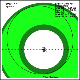
Figure 1: A top-down view of the WASP-47 system, showing the host star (intersection of the dotted cross-hairs) and the orbits of the planets (solid lines). The extent of the HZ is shown in green, where light green is the conservative HZ and dark green is the optimistic extension to the HZ.

Using the above stellar parameters, we calculate the extent of the HZ for the system. We adopt the HZ as described by Kopparapu et al. (2013, 2014), including the conservative and optimistic boundaries (Kane et al., 2013, 2016). Briefly, the demarcation of the conservative HZ is defined by the runaway greenhouse limit at the inner edge and maximum greenhouse at the outer edge, whereas the boundaries of the optimistic HZ are estimated based on empirical evidence regarding the prevalence of liquid water on the surfaces of Venus and Mars, respectively. Furthermore, the uncertainties in the HZ boundaries depend on the robustness of the stellar property values (Kane, 2014). As pointed out by Vanderburg et al. (2017), the WASP-47 stellar properties are quite accurately determined, aided substantially by the vast number of measurements and similarity to the Sun. The representation of the orbital architecture shown in Figure 1 includes a green region that indicates the extent of the HZ in the system (Kane & Gelino, 2012b). The light green represents the conservative HZ and the dark green represents the optimistic extension to the HZ. The conservative and optimistic HZ span the ranges 1.01–1.80 AU and 0.80–1.89 AU respectively.

Figure 1 indicates that, although in an eccentric orbit, the non-transiting giant planet WASP-47c remains entirely within the optimistic HZ during its orbit. Giant planets in the HZ are intrinsically interesting from the perspective of potentially habitable exomoons (see Section 5). However, they also pose intriguing dynamical questions regarding whether there could be farther out giant planets that contributed to migration halting mechanisms (Masset & Snellgrove, 2001; Pierens et al., 2014) and continuing dynamical interactions (Kane & Raymond, 2014). The current RV time series provided by Vanderburg et al. (2017) do not have a sufficient baseline to exclude the presence of further long-period giant planets, the detection of which would support the notion of dynamical interactions with a farther companion, consistent with the eccentric giant planet detected in the HZ.

3 Planetary Phase Amplitudes

The photometric variations of a star–planet system due to the orbital phase of the planet are dominated by three major effects: reflected light and thermal emission, Doppler beaming, and ellipsoidal variations (Faigler & Mazeh, 2011). The precise nature of how these various contributions to the photometric variations are weighted may be used to discriminate between planetary and stellar companions (Drake, 2003; Kane & Gelino, 2012a) and study multi-planet systems (Kane & Gelino, 2013; Gelino & Kane, 2014). The Doppler beaming and ellipsoidal variations are primarily functions of the companion mass (Loeb & Gaudi, 2003; Zucker et al., 2007), whereas the reflected light component depends upon the planet radius and atmospheric properties (Sudarsky et al., 2005) with further dependencies upon orbital parameters (Kane & Gelino, 2010, 2011b). The precision of photometry from the Kepler spacecraft has demonstrated on numerous occasions that it is sufficient to detect exoplanet phase variations (Welsh et al., 2010; Esteves et al., 2013; Angerhausen et al., 2015; Esteves et al., 2015; Shporer & Hu, 2015).

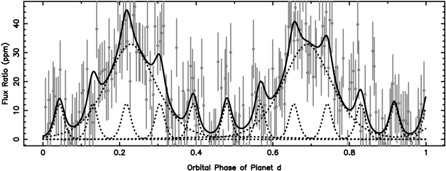
Figure 2: Simulated phase variations for the WASP-47 system and for one complete orbit of planet d (9.03 days). The dotted lines represent the phase variations for the individual planets and the solid line is the combined phase effect. The gray data points are simulated photometric measurements to provide an estimate of expected signal with a gaussian scatter of 10 ppm.

For the reflected light component observed at wavelength $\lambda$, we adopt the formalism of Kane & Gelino (2010). The star–planet separation incorporating Keplerian orbital parameters is given by

$$r=\frac{a(1-e^{2})}{1+e\cos f}$$ (1)

where $f$ is the true anomaly. The phase angle ($\alpha$) of the planet is defined to be zero when the planet is located at superior conjunction, and is given by

$$\cos\alpha=-\sin(\omega+f)$$ (2)

To describe the scattering properties of atmospheres, we adopt a phase function ($g(\alpha)$) that was empirically derived based upon Pioneer observations of Venus and Jupiter (Hilton, 1992). Combined with the geometric albedo of the planetary surface ($A_{g}(\lambda)$), these parameters together calculate the flux ratio ($\epsilon$) between the planet and star

$$\epsilon(\alpha,\lambda)\equiv\frac{f_{p}(\alpha,\lambda)}{f_{\star}(\lambda)}=A_{g}(\lambda)g(\alpha,\lambda)\frac{R_{p}^{2}}{r^{2}}$$ (3)

where $f_{p}(\alpha,\lambda)$ and $f_{\star}(\lambda)$ are the fluxes received by the observer from the planet and star respectively.

Observations and models show that planetary geometric albedos can span a large range of values, depending on surface/atmosphere composition and incident flux (Sudarsky et al., 2005; Kane & Gelino, 2010; Esteves et al., 2013). For the purposes of demonstration, we calculate planet–star flux ratios (Equation 3) for the WASP-47 planets using $A_{g}=0.3$ to represent a typical atmospheric albedo based on the Solar System planets. Since the inner planet (e) is likely terrestrial and exists under extreme incident flux conditions, we also adopt $A_{g}=0.1$ and $A_{g}=0.6$ for this planet to represent rocky (no atmosphere) and molten surfaces respectively, based upon similar surfaces observed in the Solar System and lava-ocean models (Kane et al., 2011; Rouan et al., 2011). The amplitude of the phase variations for these assumptions are shown alongside the orbital parameters in Table 1. The amplitudes demonstrate that, for the reflected light component, planet b is expected to dominate the phase variations and planets d and c are unlikely to contribute any significant phase signature.

Shown in Figure 2 is a model of the predicted phase variations of the planets in the WASP-47 system for one complete orbital period of planet d (9.03 days). The dotted lines indicate the contributions from the individual planets and the solid line represents the combined effects of all planets. In this model, all planets start at inferior conjunction where the phase amplitude is zero. We also adopt the atmosphere model for all planets except for planet e, where a molten model has been adopted. The light gray data points are simulated photometric measurements that have been convolved with a gaussian filter of width 10 ppm to emulate the expected dispersion of the data. As expected, the signature of planet b dominates the variation in the photometry with planet e producing a small but measurable effect.

It is worth considering the infrared (IR) component of the phase variations due to the thermal emission of the planets. This IR component is particularly important for modeling overall phase variations when the planet is tidal locked, whereby the view of the hot dayside varies with time (Kane & Gelino, 2011a). The IR contribution to the total observed flux depends on the bandpass of the detector. For the Kepler spacecraft, the detectors include sensitivity into IR wavelengths, roughly spanning 420–900 nm (Borucki et al., 2010). To estimate the IR flux contribution, we calculated the blackbody equilibrium temperature ($T_{\mathrm{eq}}$) for each planet and the associated flux. We then separately integrated the entire blackbody curve and the region that falls within the Kepler bandpass, allowing the calculation of the percentage thermal emission flux in the bandpass ($f_{\mathrm{IR}}$). For example, the value of $T_{\mathrm{eq}}$ for planet e is especially high (2608 K), resulting in a substantial fraction of the thermal emission (12.86%) falling within the Kepler bandpass. Thus, for planet e, the IR component may be a non-negligible amount of the photometric variations caused by the planet. The $T_{\mathrm{eq}}$ and $f_{\mathrm{IR}}$ values for all four WASP-47 planets are included in Table 1.

4 Phase Curve Analysis of the K2 Photometry

In this section we discuss our phase curve analysis and geometric albedo measurements for the planets in the WASP-47 system. In Section 4.1, we explain how we manipulate the K2 photometry. Our phase curve model and the results of the phase curve model fit to the K2 photometry are given in Section 4.2. We derive upper limits on the geometric albedo using an injection test described in Section 4.3 and show the results of the injection test in Section 4.4. Finally, in Section 4.5 we discuss how an individual planet’s significant phase curve may influence the phase curves of other planets in the WASP-47 system.

4.1 Data Treatment

To analyze the phase curves of the planets in the WASP-47 system, we use the short-cadence (58.3 s) Pre-search Data Conditioned (PDC) light curve of WASP-47 produced by the Kepler/K2 pipeline. The light curve is corrected for systematic effects, such as those caused by unstable pointing, following the procedures described by Vanderburg & Johnson (2014) and Becker et al. (2015), with the exception of removing short frequency variations that are caused by the intrinsic phase variations of the WASP-47 planets. However, some long-term variability remains in the light curve, as can be seen in the top panel of Figure 3. Therefore, we separate the light curve into two segments, normalize each segment by the best-fit 2nd degree polynomial, and remove two days of photometry at the edges of each segment in order to avoid residual systematic effects caused by the imperfect normalization that could bias our phase curve analysis. The final light curve that we use in the phase variation analysis is shown by the light blue points in the bottom panel of Figure 3.

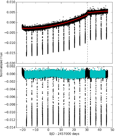
Figure 3: Top: The K2 photometry for WASP-47 after being corrected for systematic effects (Vanderburg & Johnson, 2014; Becker et al., 2015). The black vertical dashed line shows where we split the light curve into two segments, and the red curves show the best-fit 2nd-degree polynomial to the two non-transiting segments of the light curve. Bottom: The resultant light curve that has been normalized by the 2nd-degree polynomial in two segments. We use the light blue points in our phase variation analysis, which do not include transits or expected eclipses from any of the planets in WASP-47.

4.2 Phase Curve Fitting

We use the times of conjunction, orbital periods, and transit duration times reported in Vanderburg et al. (2017) to phase fold the light curve and trim the transits and expected eclipses for the b, d, and e planets. WASP-47c is not included in our phase curve analysis given that the available photometry only covers 11% of its orbital phase. Furthermore, the expected phase curve of WASP-47c is negligible compared to the expected b, d, and e planet phase curves (see Section 3). For the phase curve analysis, we adopt the BEaming, Ellipsoidal, and Reflection (BEER) model developed by Faigler & Mazeh (2011). This model can be described as a simple, double harmonic sinusoidal model, such that the flux ($F$) as a function of phase ($\phi$) is given by

where $A_{\mathrm{norm}}$ is a normalization offset and $A_{\mathrm{beam}}$, $A_{\mathrm{ellip}}$, and $A_{\mathrm{refl}}$ are the semi-major amplitudes of the beaming, ellipsoidal, and reflection effects, respectively. The semi-amplitudes of the beaming and ellipsoidal variations could be estimated and held fixed in the model based on the known stellar and planetary parameters of WASP-47 and its companions. However, we choose to leave these effects as free parameters in the fitting due to the ellipsoidal distortion of stars not being well understood (e.g., Shporer, 2017) and the beaming effect being degenerate with a phase-shifted reflection component. The signs of the amplitudes in Equation LABEL:beereqn are also allowed to be free in our fitting, but for the best-fit model to be physically represented by the BEER model, the reflection and ellipsoidal best-fit semi-amplitudes should be negative (equivalent to a 180 degree phase shift). The geometric albedo ($A_{g}$) in the Kepler bandpass can be measured for each planet using the strength of the reflection component by

$$A_{g}=\frac{A_{\text{refl}}}{\sin{i}}\left(\frac{R_{p}}{a}\right)^{-2}\text{.}$$ (5)

Since the b, d, and e planets all transit WASP-47, we consider the effect of the inclination to be negligible and set $\sin{i}$ to unity. A least-squares minimization technique is used to find the best-fit BEER model. Outlier removal is iterative, in that any data that are $>$4.5$\sigma$ different from the model are removed, then the best-fit BEER model is reevaluated. The remaining data are divided into 100 bins of the planet phase, then fit with the BEER model to ensure consistency between the best-fit models.

The best-fit BEER model is based on the shape of the light curve alone and is not informed by the stellar or planetary parameters. The stellar and planetary parameters are then typically used alongside the measured semi-amplitudes of the BEER model to extract the planet’s albedo. We show the best-fit BEER model phase curves for the WASP-47 b and e planets in Figure 4.2. The best-fit phase curve of WASP-47d is not shown since we find no evidence for BEER-related effects based on the significance and signs of the best-fit semi-amplitudes. We find that the measured phase curves of the b and e planets do not significantly deviate from a flat line, therefore we conclude that their phase curves are likely consistent with having a very low albedo (Equation 5). In Section 4.3, we aim to constrain the upper limit of the geometric albedos of the b and e planets by injecting the expected phase curve model into the raw K2 photometry for different assumed albedos.

Figure 4: Best-fit BEER model phase curves for the b (top row) and e (bottom row) planets in WASP-47, from which the phase curves are determined to be undetected (see Section 4.2). The red points show the binned K2 photometry. The thick black and thin yellow curves show the BEER models that are best-fit to the unbinned (not shown) and binned (red points) photometry, respectively. The individual components of the BEER model are shown by the blue (reflection), green (beaming), and purple (ellipsoidal) curves. The thin horizontal black line indicates the average flux of the data and is used to compare the phase curve to a flat line. The significance of the best-fit model compared to a flat line is listed at the top of each panel.

4.3 Injection Test

Table 2: Injected and Recovered Phase Variation Amplitudes^†

Planet	Injected Phase Curve					Recovered Phase Curve
	$A_{\text{beam}}$	$A_{\text{ellip}}$	$A_{\text{refl}}$	$A_{g}$		$A_{\text{refl}}$	$A_{g}$	$\chi^{2}_{\nu\text{,line}}$	$\chi^{2}_{\nu\text{,BEER}}$	$\chi^{2}_{\nu\text{,diff}}$
	(ppm)	(ppm)	(ppm)			(ppm)
b	1.68	-1.50	-14.76	0.17		-19.12	0.18	4.09	3.08	1.01
			-37.96	0.36		-35.23	0.33	6.35	3.25	3.10
e	0.06	-0.78	-13.50	0.68		-12.61	0.64	3.01	2.51	0.5
			-19.85	1.00		-17.29	0.87	3.31	2.48	0.83

Considering the nature of the systematic effects in the K2 photometry (e.g., reaction wheel jitter and solar pressure induced drift), it is possible that the phase variations are removed when the light curve is corrected. Therefore, we investigate whether a BEER-like phase curve could be recovered when the predicted phase variations are injected into the raw K2 light curve for the WASP-47 b, d, and e planets. We assume the stellar and planetary parameters reported by Vanderburg et al. (2017) and use the expressions from Faigler & Mazeh (2011) to estimate the semi-amplitudes of the beaming ($A_{\mathrm{beam}}$) and ellipsoidal ($A_{\mathrm{ellip}}$) effects, although these signals are $<$2 ppm for all planets in the WASP-47 system (see Table 2) and is the same for all injection tests. The only difference between each injected phase curve test was the strength of each planet’s reflectivity. The semi-amplitude of the reflection effect ($A_{\mathrm{refl}}$) for each planet is determined by Equation 5 in steps of 0.01 albedo. For each injection test, we add the combined phase curve (Equation LABEL:beereqn) of all three planets to the raw K2 photometry. For simplicity, we assume that all of the planets have the same albedo for each injection test. We then repeat the K2 corrections described by Vanderburg & Johnson (2014), our 2nd degree polynomial normalization on the two light curve segments, and our phase curve analysis.

Figure 5: The results of the phase variation analysis of the WASP-47 b (top two panels) and e (bottom two panels) planets. For each of the two planets, the top panel indicates the reduced chi-squared for the best-fit BEER model (red points), a horizontal line model (yellow points), and their difference (black points). The values for the reduced chi-squared of the two models are offset vertically for clarity. The bottom panel shows a comparison between the injected albedo and the recovered (measured) albedo. The thin solid black line shows where the recovered albedos equal the injected albedos. For the b planet, the bottom panel also includes a thick light blue line underneath the black points that is fit to the recovered versus injected albedos. The thick light blue line emphasizes the vertical offset from equally recovered and injected albedos, which we interpret as a tentative 0.016 geometric albedo for WASP-47b.

4.4 Results

We find that the phase curve injections in steps of 0.01 albedo result in increasingly higher recovered albedo measurements, as expected, for the b and e planets. The WASP-47d phase curve, on the other hand, remains inconsistent with the BEER model based on the significance and signs of the measured semi-amplitudes, even when the maximum albedo ($A_{g}=1$) is injected. In order to quantify the significance of the models that were fit to the injected phase curve photometry, we measure the difference between the reduced chi-squared ($\chi_{\nu}^{2}$) of a horizontal line at the average flux of the data ($\chi^{2}_{\nu\text{,line}}$) and the reduced chi-squared of the best-fit BEER model ($\chi^{2}_{\nu\text{,BEER}}$). Figure 4.3 shows the reduced chi-squared of the two models, their difference, and the extracted albedo as a function of the injected albedo for the b and e planets of WASP-47.

As can be seen by the top panels of Figure 4.3, the extracted albedos for WASP-47b are incredibly consistent with the injected albedos. Furthermore, there is an underlying offset in the extracted albedos, such that the extracted albedos are on average 0.016 higher than the injected albedos. This offset could be caused by each injected phase curve being added on top of the underlying phase curve of WASP-47b. Since all BEER effects are left as free parameters in the injection test phase curve fitting, the injected BEER effects are assumed to be added to the intrinsic phase curve that was undetected in Figure 4.2. Therefore, based on the offset between the injected and recovered albedos in Figure 4.3, we infer a potential geometric albedo of 0.016 for WASP-47b. However, this tentative 0.016 albedo is less than the 0.026 scatter of the extracted albedos. We infer $1\sigma$ and $3\sigma$ upper limits on the geometric albedo of WASP-47b based on the significance of the measured BEER phase curve from the injection tests. We define statistical significance using the difference between the reduced chi-squared for the horizontal line and BEER models ($\chi^{2}_{\nu\text{,diff}}=\chi^{2}_{\nu\text{,line}}-\chi^{2}_{\nu\text{,BEER}}$). We use a $\chi^{2}_{\nu\text{,diff}}$ of 1 and 3 to infer that the $1\sigma$ and $3\sigma$ upper limits of the WASP-47b geometric albedo are 0.17 and 0.36, respectively. The semi-amplitudes, albedos, and reduced chi-squared values of the injected and recovered phase curves based on the 0.17 and 0.36 albedo injection tests for WASP-47b are given in Table 2 and the respective best-fit phase curves are shown in the top panels of Figure 6.

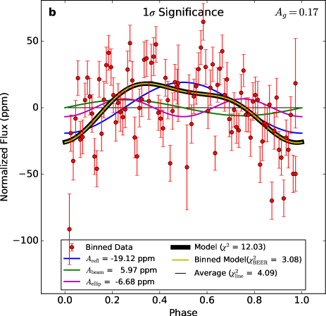
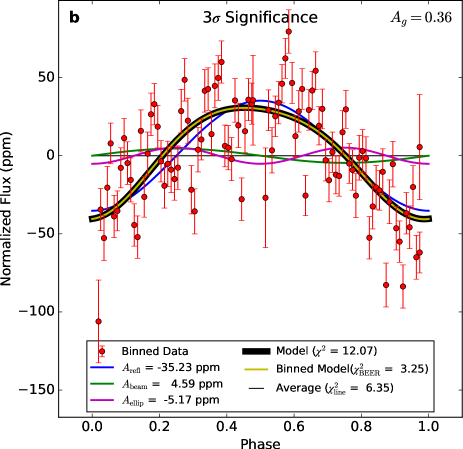
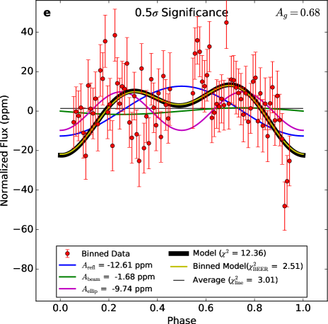
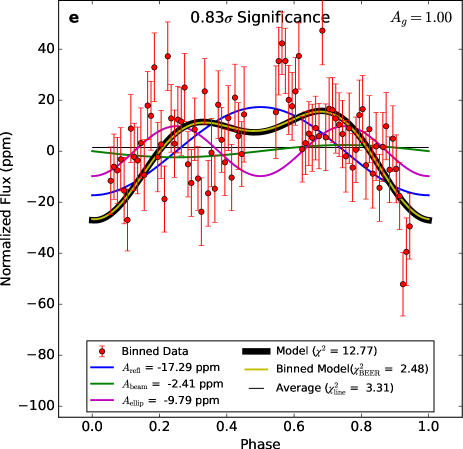
Figure 6: Results of the BEER model phase curve injection tests (see Sections 4.3 and 4.4) that were used to infer upper limits on the albedos of the b (top row) and e (bottom row) planets in WASP-47. The red points show the binned K2 photometry that has been injected with the expected phase curve for a given geometric albedo, which is listed in the top right corner of each panel. The thick black and thin yellow curves show the best-fit BEER models to the unbinned (not shown) and binned (red points) photometry, respectively. The individual components of the BEER model are shown by the blue (reflection), green (beaming), and purple (ellipsoidal) curves. The thin horizontal black line indicates the average flux of the data and is used to compare the phase curve to a flat line. The significance of the best-fit model compared to a flat line is listed at the top of each panel. All corresponding injected and recovered semi-amplitudes, albedos, and reduced chi-squared values are reported in Table 2.

Initially, the recovered albedo measurements for WASP-47e were systematically lower than the injected albedos. The intrinsic phase curve of WASP-47e cannot explain the lower albedo measurements. The phase variations of WASP-47e may be undetectable or removed when correcting the K2 photometry, especially considering that the realignment of the K2 spacecraft occurred approximately on the same timescale as the orbit of the e planet. The phase curve fit is also sensitive to the input transit duration time. In addition to removing the expected transits and occultations, the transit duration time also affects how much of the out-of-transit light curve is included in the fit near 0 and 0.5 phase. These phases also represent minima and maxima of the reflection and ellipsoidal variations, such that the inclusion of in-transit photometry or the exclusion of too much of the out-of-transit photometry could affect the measured semi-amplitudes of these effects. We found that reducing the transit duration time by 15 minutes ($t_{14}=1.7$ hr) results in the best recovered albedos compared to the injected albedos. The reduced chi-squared statistics and the recovered versus injected albedos are shown in the bottom panels of Figure 4.3. Oddly, there is a 0.75 slope between the extracted and injected albedos for WASP-47e. We suspect that the discrepancy between the extracted and injected albedos could be attributed to (1) the injected phase curve being altered by the corrections to the K2 photometry that are on approximately the same timescale as the orbital period of the e planet, (2) the injected phase curve being added to the underlying intrinsic phase curve, or (3) a combination thereof. Regardless, we cannot constrain the geometric albedo of WASP-47e as we did for WASP-47b, since the difference between the reduced chi-squared of the horizontal line and BEER models never exceeds unity (i.e., $\chi^{2}_{\nu\text{,diff}}$ is always $<$1). Therefore, the injected phase curve photometry and the best-fit recovered phase curves shown in the bottom panels of Figure 6 are based on the injection tests that result from (1) the best-fit BEER phase curve being detected at a 0.5$\sigma$ significance that infers an albedo of 0.68, and (2) injecting a BEER phase curve with a maximum geometric albedo of $A_{g}=1.0$ (0.83$\sigma$ significance). The semi-amplitudes, albedos, and reduced chi-squared values of the respective injected and recovered phase curves are given in Table 2.

4.5 Potential Blended Phase Curves

For multi-planet systems with planets that are in resonant orbits, there may be concern that a strong phase variation signature of one planet may be blended with the phase curves of other planets in the system. None of the known planets in WASP-47 are in resonance with each other, but for completeness we investigate whether a strong injected phase curve of an individual planet influences the phase curves of other planets in the system. Since the phase curve of WASP-47e is not significantly detected ($<$1$\sigma$) at an albedo of 1, we inject a phase curve with an unphysically high geometric albedo equal to 10 for all of the planets together, then the b, d, and e planets individually. For each of these injection cases, we repeat our phase curve analysis on the b, d, and e planets to see how a strong reflection modulation may influence the phase curves of the other planets in the system.

The shape of the WASP-47d phase curve remains generally the same in all test cases, but is most significantly modified by a strong injected phase curve of the b planet. This is because the b planet has the strongest phase curve signature of all the planets in the WASP-47 system and it is near a 2:1 resonance with the d planet. However, in all cases the WASP-47d phase curve remains inconsistent with a BEER model based on the significance and sign of the measured semi-amplitudes. Since WASP-47b exhibits the strongest phase variation signature, the changes to its phase curve are negligible regardless of whether the contributions from the phase curves of the other planets are included. Curiously, when only the WASP-47e phase curve is injected, the recovered albedo is lower than when all phase curves are included. Once again, the extracted albedo is lower than the injected albedo for WASP-47e, suggesting that the intrinsic phase curve is suppressed by the low signal-to-noise or the corrections of the K2 photometry that are approximately on the same timescale as the orbit of the e planet.

5 Discussion

As described in Section 3, analysis of potential exoplanet phase signatures have been carried out by numerous groups. In many cases, the albedo measurements, or upper limits, have led to the conclusion that hot Jupiters tend to have very low albedos (Rowe et al., 2008; Bell et al., 2017; Močnik et al., 2018; Mallonn et al., 2019) due to significant constraints on the presence of icy condensates in the atmospheres of such planets. Note that Rowe et al. (2008) and Močnik et al. (2018) establish the low albedo estimates through analysis of the out-of-transit/eclipse phase variations rather than just eclipse measurements, similar to the methodology we present here. There exist exceptions to low albedos for hot Jupiters however, such as Kepler-7b (Demory et al., 2011), no doubt reflecting the diversity of possible atmospheric compositions. Our results for WASP-47b are consistent with the majority of cases where the planets are demonstrated to have poorly reflective atmospheres. The Neptune-size WASP-47d planet lies well below the detection capabilities of the K2 data, as predicted by the calculations shown in Table 1, but may also have a blended phase curve due to a near 2:1 resonance with the stronger phase curve of the b planet. In the case of the e planet, the calculations of Table 1 indicate that the phase signature could be detected if the planet is highly reflective, such as a molten surface. Our analyses in Section 4 show that the e planet phase curve lies at the threshold of K2 photometric detectability, possibly due to photometric corrections for the periodic ($\sim$1 day) pointing alignment of the spacecraft being on a similar timescale as the orbit of the e planet ($P=0.79$ days). The diversity of geometric albedos is expected to be higher for terrestrial planets due to the diversity of surfaces and atmospheres. Hot terrestrial planets like WASP-47e may have a limited variety of reflective properties since the high incident flux can potentially erode atmospheres (Tian, 2009; Roettenbacher & Kane, 2017; Zahnle & Catling, 2017; Brogi, 2018) as well as create molten surface environments.

We investigated the possibility of additional photometry of WASP-47 from other facilities, such as the Transiting Exoplanet Survey Satellite (TESS), described in detail by Ricker et al. (2015). WASP-47 has ecliptic coordinates of 328.996$\arcdeg$ longitude and -0.209$\arcdeg$ latitude. Being so close to the ecliptic, the star does not coincide with TESS observations during the primary mission, though it will likely be observed in extended mission scenarios that target the ecliptic region of the sky (Sullivan et al., 2015). Furthermore, WASP-47 is bright enough to serve as an excellent target for follow-up observations using the CHaracterising ExOPlanets Satellite (CHEOPS), which was launched in early 2020 (Broeg et al., 2014). Observations of WASP-47 using both TESS and CHEOPS brings a significant advantage in multi-wavelength observations of atmospheric phase signatures since, as noted in Section 3, the reflected light component is wavelength dependant (Gaidos et al., 2017). Note also that the most significant correction to the K2 photometry described in Section 4 is for the unstable pointing, which is on the order of $\sim$1 day and is similar to the orbital period of WASP-47e. This further emphasizes the advantage of follow-up observations from a more stable spacecraft such as TESS or CHEOPS.

The dynamical evolution of the known planets in the WASP-47 system is, on its own, a fascinating aspect of the system. The compact nature of the known inner three planets is relatively unperturbed by the presence of planet c in an eccentric orbit within the HZ. As described in Section 2, further acquisition of RV data may reveal an additional planet in a longer period orbit, well outside of the HZ. If so, the farther giant planet could be regularly exchanging angular momentum through oscillation of eccentricities, as has been observed in other systems (Kane & Raymond, 2014). Given the discovery history of the system, it is likely that there are yet further planet discoveries to be made in the system with additional RV monitoring.

WASP-47c is a gas giant and so is not deemed habitable on its own, but it does have the potential to be the host of large rocky exomoons that would also be in the HZ. An exomoon would have the benefit of a diversity of sources providing energy to their potential biosphere, not just a reliance on the flux received from the host star. The reflected light and emitted heat of the host planet as well as tidal heating forces caused by the motion of the moon orbiting the planet will provide additional energy to a moon (Heller & Barnes, 2013; Hinkel & Kane, 2013). These combined heating effects effectively extend the HZ for these moons, creating a wider temperate area in which they may maintain conditions on their surface that are amenable to liquid surface water (Scharf, 2006). For a planet like WASP-47c that spends part of its orbit near the outer edge of the HZ (see Figure 1), these extra energy sources may enable potential exomoons in orbit to maintain habitable conditions during apastron.

While there have been preliminary detections of exomoon signatures (Teachey et al., 2018; Teachey & Kipping, 2018) no exomoons have been confirmed to date (Heller et al., 2019; Kreidberg et al., 2019). However, there is a general consensus in the community that the existence of exomoons is likely (Williams et al., 1997; Kipping et al., 2009; Heller, 2012; Heller & Pudritz, 2015; Zollinger et al., 2017) and it has even been proposed that there could be as many or even more exomoons in the HZ as there are terrestrial planets (Hill et al., 2018).

Any potentially habitable moon would need to have a large enough mass to maintain an atmosphere that can support liquid surface water, and may need a magnetosphere to protect its atmosphere and surface from the radiation emitted by the host planet and potentially needs tectonic plates to facilitate carbon cycling (Williams et al., 1997). It has been posed by Heller & Barnes (2013) that a moon would need to be at least $\geq 0.25M\oplus$ to maintain these conditions. Using the relationship derived in Canup & Ward (2002), the maximum mass of a moon that is formed in situ with WASP-47 c is $\sim$0.04 $M_{\oplus}$. Therefore it is likely that for a moon to be considered habitable about this planet, it would need to have been captured rather than formed in situ with the planet (Williams, 2013).

6 Conclusions

The WASP-47 system has been described as “the gift that keeps on giving,” with numerous exoplanet discoveries beyond the initial discovery of the hot Jupiter, WASP-47b. The orbital architecture of the system that combines compact orbits with a giant planet in an eccentric orbit in the HZ presents an interesting dynamical configuration. As discussed in this paper, the HZ giant planet is a potential abode for exomoons and may represent a common scenario of giant planet migration into the HZ that can truncate HZ terrestrial planet occurrence rates (Hill et al., 2018). The eccentric nature of the giant planet orbit may be indicative of past planet-planet scattering (Carrera et al., 2019) or an ongoing interaction with a more distant, yet undiscovered, planet (Kane & Raymond, 2014). The complete orbital architecture remains open with the likelihood of at least one additional planet in the system.

However, the most prominent source of new discoveries within the system may originate from atmospheric studies of the inner transiting planets of the system. The architecture of an inner super-Earth followed by a gas giant planet has been observed in other systems, such as 55 Cancri (Kane et al., 2011), and may be related to planet formation processes in compact systems (Weiss et al., 2018). This combination of a relatively small inner planet with a gas giant neighbor is compelling from a phase variation point of view since the planets can have similar phase amplitudes. Our calculations have shown that planet e with a lava surface can have a comparable phase amplitude to planet b if that planet is of particularly low albedo. Our analysis of the K2 photometry demonstrates that planet b must have a very low albedo, consistent with albedo measurements and/or constraints for other short period giant planets. The phase signature of planet e lies barely beneath the statistically significant detection threshold of the K2 photometry, but our injection test and subsequent analysis shows that the difference in reduced chi-squared for the BEER model diverges for a broad range of injected albedos.

The plethora of dark planets in exoplanetary systems, such as WASP-47b, will present an interesting sample from which to study the relationship between atmospheric composition and geometric albedo. Systems such as WASP-47 and those similar systems with bright host stars discovered with TESS will thus provide a concise target set from which to form the basis of a transmission spectroscopy study with the James Webb Space Telescope (Kempton et al., 2018) and may also be possible for terrestrial targets such as WASP-47e (Batalha et al., 2018). It is thus expected that the continued monitoring of WASP-47 and uncovering architecturally similar systems has a great deal more to teach us about the planet formation, evolution, and planetary atmospheres.

References

- Agol et al. (2005) Agol, E., Steffen, J., Sari, R., & Clarkson, W. 2005, MNRAS, 359, 567
- Almenara et al. (2016) Almenara, J. M., Díaz, R. F., Bonfils, X., & Udry, S. 2016, A&A, 595, L5
- Angerhausen et al. (2015) Angerhausen, D., DeLarme, E., & Morse, J. A. 2015, PASP, 127, 1113
- Batalha et al. (2018) Batalha, N. E., Lewis, N. K., Line, M. R., Valenti, J., & Stevenson, K. 2018, ApJ, 856, L34
- Becker et al. (2015) Becker, J. C., Vanderburg, A., Adams, F. C., Rappaport, S. A., & Schwengeler, H. M. 2015, ApJ, 812, L18
- Bell et al. (2017) Bell, T. J., Nikolov, N., Cowan, N. B., et al. 2017, ApJ, 847, L2
- Borucki et al. (2010) Borucki, W. J., Koch, D., Basri, G., et al. 2010, Science, 327, 977
- Broeg et al. (2014) Broeg, C., Benz, W., Thomas, N., & Cheops Team. 2014, Contributions of the Astronomical Observatory Skalnate Pleso, 43, 498
- Brogi (2018) Brogi, M. 2018, Science, 362, 1360
- Canup & Ward (2002) Canup, R. M., & Ward, W. R. 2002, AJ, 124, 3404
- Carrera et al. (2019) Carrera, D., Raymond, S. N., & Davies, M. B. 2019, A&A, 629, L7
- Dai et al. (2015) Dai, F., Winn, J. N., Arriagada, P., et al. 2015, ApJ, 813, L9
- Demory et al. (2011) Demory, B.-O., Seager, S., Madhusudhan, N., et al. 2011, ApJ, 735, L12
- Drake (2003) Drake, A. J. 2003, ApJ, 589, 1020
- Esteves et al. (2013) Esteves, L. J., De Mooij, E. J. W., & Jayawardhana, R. 2013, ApJ, 772, 51
- Esteves et al. (2015) —. 2015, ApJ, 804, 150
- Faigler & Mazeh (2011) Faigler, S., & Mazeh, T. 2011, MNRAS, 415, 3921
- Ford (2014) Ford, E. B. 2014, Proceedings of the National Academy of Science, 111, 12616
- Fulton et al. (2018) Fulton, B. J., Petigura, E. A., Blunt, S., & Sinukoff, E. 2018, PASP, 130, 044504
- Funk et al. (2010) Funk, B., Wuchterl, G., Schwarz, R., Pilat-Lohinger, E., & Eggl, S. 2010, A&A, 516, A82
- Gaidos et al. (2017) Gaidos, E., Kitzmann, D., & Heng, K. 2017, MNRAS, 468, 3418
- Gelino & Kane (2014) Gelino, D. M., & Kane, S. R. 2014, ApJ, 787, 105
- Hands et al. (2014) Hands, T. O., Alexander, R. D., & Dehnen, W. 2014, MNRAS, 445, 749
- Hatzes (2016) Hatzes, A. P. 2016, Space Sci. Rev., 205, 267
- Heller (2012) Heller, R. 2012, A&A, 545, L8
- Heller & Barnes (2013) Heller, R., & Barnes, R. 2013, Astrobiology, 13, 18
- Heller & Pudritz (2015) Heller, R., & Pudritz, R. 2015, ApJ, 806, 181
- Heller et al. (2019) Heller, R., Rodenbeck, K., & Bruno, G. 2019, A&A, 624, A95
- Hellier et al. (2012) Hellier, C., Anderson, D. R., Collier Cameron, A., et al. 2012, MNRAS, 426, 739
- Hill et al. (2018) Hill, M. L., Kane, S. R., Seperuelo Duarte, E., et al. 2018, ApJ, 860, 67
- Hilton (1992) Hilton, J. L. 1992, Explanatory Supplement to the Astronomical Almanac, ed. Seidelmann, P.K. (University Science Books, Mill Valley CA), p. 383
- Hinkel & Kane (2013) Hinkel, N. R., & Kane, S. R. 2013, ApJ, 774, 27
- Holman & Murray (2005) Holman, M. J., & Murray, N. W. 2005, Science, 307, 1288
- Howell et al. (2014) Howell, S. B., Sobeck, C., Haas, M., et al. 2014, PASP, 126, 398
- Kane (2014) Kane, S. R. 2014, ApJ, 782, 111
- Kane et al. (2013) Kane, S. R., Barclay, T., & Gelino, D. M. 2013, ApJ, 770, L20
- Kane et al. (2012) Kane, S. R., Ciardi, D. R., Gelino, D. M., & von Braun, K. 2012, MNRAS, 425, 757
- Kane & Gelino (2010) Kane, S. R., & Gelino, D. M. 2010, ApJ, 724, 818
- Kane & Gelino (2011a) —. 2011a, ApJ, 741, 52
- Kane & Gelino (2011b) —. 2011b, ApJ, 729, 74
- Kane & Gelino (2012a) —. 2012a, MNRAS, 424, 779
- Kane & Gelino (2012b) —. 2012b, PASP, 124, 323
- Kane & Gelino (2013) —. 2013, ApJ, 762, 129
- Kane et al. (2011) Kane, S. R., Gelino, D. M., Ciardi, D. R., Dragomir, D., & von Braun, K. 2011, ApJ, 740, 61
- Kane & Raymond (2014) Kane, S. R., & Raymond, S. N. 2014, ApJ, 784, 104
- Kane & Torres (2017) Kane, S. R., & Torres, S. M. 2017, AJ, 154, 204
- Kane & von Braun (2008) Kane, S. R., & von Braun, K. 2008, ApJ, 689, 492
- Kane et al. (2016) Kane, S. R., Hill, M. L., Kasting, J. F., et al. 2016, ApJ, 830, 1
- Kempton et al. (2018) Kempton, E. M. R., Bean, J. L., Louie, D. R., et al. 2018, PASP, 130, 114401
- Kipping et al. (2009) Kipping, D. M., Fossey, S. J., & Campanella, G. 2009, MNRAS, 400, 398
- Kopparapu et al. (2014) Kopparapu, R. K., Ramirez, R. M., SchottelKotte, J., et al. 2014, ApJ, 787, L29
- Kopparapu et al. (2013) Kopparapu, R. K., Ramirez, R., Kasting, J. F., et al. 2013, ApJ, 765, 131
- Kreidberg et al. (2019) Kreidberg, L., Luger, R., & Bedell, M. 2019, ApJ, 877, L15
- Loeb & Gaudi (2003) Loeb, A., & Gaudi, B. S. 2003, ApJ, 588, L117
- Madhusudhan et al. (2017) Madhusudhan, N., Bitsch, B., Johansen, A., & Eriksson, L. 2017, MNRAS, 469, 4102
- Mallonn et al. (2019) Mallonn, M., Köhler, J., Alexoudi, X., et al. 2019, A&A, 624, A62
- Masset & Snellgrove (2001) Masset, F., & Snellgrove, M. 2001, MNRAS, 320, L55
- Močnik et al. (2018) Močnik, T., Hellier, C., & Southworth, J. 2018, AJ, 156, 44
- Neveu-VanMalle et al. (2016) Neveu-VanMalle, M., Queloz, D., Anderson, D. R., et al. 2016, A&A, 586, A93
- Pierens et al. (2014) Pierens, A., Raymond, S. N., Nesvorny, D., & Morbidelli, A. 2014, ApJ, 795, L11
- Ricker et al. (2015) Ricker, G. R., Winn, J. N., Vanderspek, R., et al. 2015, Journal of Astronomical Telescopes, Instruments, and Systems, 1, 014003
- Roettenbacher & Kane (2017) Roettenbacher, R. M., & Kane, S. R. 2017, ApJ, 851, 77
- Rouan et al. (2011) Rouan, D., Deeg, H. J., Demangeon, O., et al. 2011, ApJ, 741, L30
- Rowe et al. (2008) Rowe, J. F., Matthews, J. M., Seager, S., et al. 2008, ApJ, 689, 1345
- Scharf (2006) Scharf, C. A. 2006, ApJ, 648, 1196
- Shporer (2017) Shporer, A. 2017, PASP, 129, 072001
- Shporer & Hu (2015) Shporer, A., & Hu, R. 2015, AJ, 150, 112
- Sinukoff et al. (2017) Sinukoff, E., Howard, A. W., Petigura, E. A., et al. 2017, AJ, 153, 70
- Sudarsky et al. (2005) Sudarsky, D., Burrows, A., Hubeny, I., & Li, A. 2005, ApJ, 627, 520
- Sullivan et al. (2015) Sullivan, P. W., Winn, J. N., Berta-Thompson, Z. K., et al. 2015, ApJ, 809, 77
- Teachey & Kipping (2018) Teachey, A., & Kipping, D. M. 2018, Science Advances, 4, eaav1784
- Teachey et al. (2018) Teachey, A., Kipping, D. M., & Schmitt, A. R. 2018, AJ, 155, 36
- Tian (2009) Tian, F. 2009, ApJ, 703, 905
- Vanderburg & Johnson (2014) Vanderburg, A., & Johnson, J. A. 2014, PASP, 126, 948
- Vanderburg et al. (2017) Vanderburg, A., Becker, J. C., Buchhave, L. A., et al. 2017, AJ, 154, 237
- Weiss et al. (2017) Weiss, L. M., Deck, K. M., Sinukoff, E., et al. 2017, AJ, 153, 265
- Weiss et al. (2018) Weiss, L. M., Marcy, G. W., Petigura, E. A., et al. 2018, AJ, 155, 48
- Welsh et al. (2010) Welsh, W. F., Orosz, J. A., Seager, S., et al. 2010, ApJ, 713, L145
- Williams (2013) Williams, D. M. 2013, Astrobiology, 13, 315
- Williams et al. (1997) Williams, D. M., Kasting, J. F., & Wade, R. A. 1997, Nature, 385, 234
- Winn & Fabrycky (2015) Winn, J. N., & Fabrycky, D. C. 2015, ARA&A, 53, 409
- Wolf (2017) Wolf, E. T. 2017, ApJ, 839, L1
- Zahnle & Catling (2017) Zahnle, K. J., & Catling, D. C. 2017, ApJ, 843, 122
- Zollinger et al. (2017) Zollinger, R. R., Armstrong, J. C., & Heller, R. 2017, MNRAS, 472, 8
- Zucker et al. (2007) Zucker, S., Mazeh, T., & Alexander, T. 2007, ApJ, 670, 1326