Adapting Planck’s route to investigate the thermodynamics
of the spin-half pyrochlore Heisenberg antiferromagnet

Abstract

The spin-half pyrochlore Heisenberg antiferromagnet (PHAF) is one of the most challenging problems in the field of highly frustrated quantum magnetism. Stimulated by the seminal paper of M. Planck [M. Planck, Verhandl. Dtsch. phys. Ges. 2, 202-204 (1900)] we calculate thermodynamic properties of this model by interpolating between the low- and high-temperature behavior. For that we follow ideas developed in detail by B. Bernu and G. Misguich and use for the interpolation the entropy exploiting sum rules [the “entropy method” (EM)]. We complement the EM results for the specific heat, the entropy, and the susceptibility by corresponding results obtained by the finite-temperature Lanczos method (FTLM) for a finite lattice of $N=32$ sites as well as by the high-temperature expansion (HTE) data. We find that due to pronounced finite-size effects the FTLM data for $N=32$ are not representative for the infinite system below $T\approx 0.7$. A similar restriction to $T\gtrsim 0.7$ holds for the HTE designed for the infinite PHAF. By contrast, the EM provides reliable data for the whole temperature region for the infinite PHAF. We find evidence for a gapless spectrum leading to a power-law behavior of the specific heat at low $T$ and for a single maximum in $c(T)$ at $T\approx 0.25$. For the susceptibility $\chi(T)$ we find indications of a monotonous increase of $\chi$ upon decreasing of $T$ reaching $\chi_{0}\approx 0.1$ at $T=0$. Moreover, the EM allows to estimate the ground-state energy to $e_{0}\approx-0.52$.

I Introduction

A paradigmatic highly frustrated spin model is the pyrochlore Heisenberg antiferromagnet (PHAF). The pyrochlore lattice is built of corner-sharing tetrahedra, see Fig. 1, below. There are several compounds where the magnetic atoms reside on the sites of the pyrochlore lattice and the exchange interaction is antiferromagnetic, see, e.g., Refs. Gardner et al. (2010); Gingras and McClarty (2014); Rau and Gingras (2019).

Already the classical PHAF (i.e., for spin $S\to\infty$) exhibits interesting properties and its study is far from being trivial Reimers et al. (1991); Reimers (1992); Moessner and Chalker (1998a, b); Isakov et al. (2004); Henley (2010); Lapa and Henley (2012). Thus, the ground-state manifold is highly degenerate, the model exhibits strong short-range correlations, but it does not exhibit any long-range order, and, because of the huge degeneracy of the ground state, the model is very susceptible to various perturbations.

The quantum spin $S=1/2$ PHAF is even more complicated. Thus, so far no accurate values for the ground-state energy $e_{0}$ for this model are available. On the one hand, the $S=1/2$ case opens the route to new quantum phases Iqbal et al. (2019). On the other hand, such powerful straightforward numerical tools like standard quantum Monte Carlo or molecular dynamics simulations are not applicable for the $S=1/2$ PHAF. Moreover, several approximation methods developed for one- and two-dimensional quantum spin systems (e.g., density matrix renormalization group and tensor network methods) are very limited in three dimensions.

Theoretical studies of the quantum PHAF are mostly focused on ground-state properties, see, e.g., Harris et al. (1991); Isoda and Mori (1998); Canals and Lacroix (1998, 2000); Koga and Kawakami (2001); Tsunetsugu (2001a, b); Berg et al. (2003); Moessner et al. (2006); Tchernyshyov et al. (2006); Kim and Han (2008); Burnell et al. (2009); Chandra and Sahoo (2018); Iqbal et al. (2019); Müller et al. (2019), whereas much less attention has been paid to its finite-temperature properties. One reason for that is the lack of methods to study thermodynamics of three-dimensional frustrated quantum spin systems. Among the few papers studying the thermodynamics of the $S=1/2$ PHAF we mention bold diagrammatic Monte Carlo simulations (stochastic sampling of all skeleton Feynman diagrams) down to the temperature $J/6$ Huang et al. (2016). This paper reports data for the susceptibility $\chi(T)$ but no data for the specific heat $c(T)$. We will refer to these data for $\chi(T)$ in Sec. IV.2. A comprehensive analysis of the spin-$S$ $J_{1}-J_{2}$ Heisenberg model by employing the pseudofermion functional renormalization group technique was presented in Ref. Iqbal et al. (2019). However, this paper does not contain data for $\chi(T)$ and $c(T)$. Finally, we mention the high-temperature expansion study and the rotation-invariant Green’s function study of the $S=1/2$ PHAF Schmidt et al. (2011); Müller et al. (2019). In these recent papers Huang et al. (2016); Iqbal et al. (2019); Müller et al. (2019) no evidence for a finite-temperature phase transition was found, i.e., the spin-half PHAF is most likely a three-dimensional spin system without singularities in the specific heat and the susceptibility.

The goal of the present paper is to study the thermodynamics of the $S=1/2$ PHAF for the whole temperature region focussing on the specific heat $c(T)$ and the static uniform susceptibility $\chi(T)$, both being basic and easily accessible quantities in experimental studies of PHAF compounds. To deal with the above mentioned challenges when studying the finite-temperature properties of the $S=1/2$ PHAF, we follow M. Planck’s ideas of his seminal paper in 1900 Planck (1900), see also Appendix A, and perform a sophisticated interpolation between the low- and high-temperature behavior of a thermodynamic potential, namely, the entropy $s$ as a function of internal energy $e$. For that we exploit also sum rules valid for the specific heat as proposed by B. Bernu and G. Misguich Bernu and Misguich (2001); Misguich and Bernu (2005), for details see Sec. III.1. In what follows we call this approach the entropy method (EM). We complement our studies based on the EM by using the finite-temperature Lanczos method (FTLM) for a finite pyrochlore lattice of $N=32$ sites and the high-temperature expansion (HTE) up to order 13.

In the present paper, we estimate the ground-state energy to $e_{0}\approx-0.52$ and find evidence for a gapless spectrum, i.e., for a power-law behavior of the specific heat at low temperatures, and for a single maximum in $c(T)$ at about 25% of the exchange coupling.

The manuscript is organized as follows. We begin with introducing the model (Sec. II) and the description of the exploited methods (Sec. III). We report our findings obtained by the FTLM (finite lattices) and by the HTE and EM (infinite lattice) in Sec. IV. We summarize our results in Sec. V.

II Model

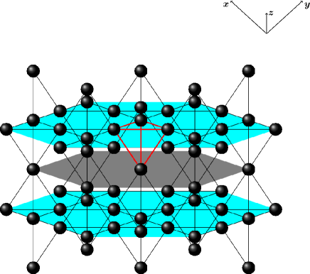
Figure 1: The pyrochlore lattice visualized here as a three-dimensional structure which consists of alternating kagome (cyan) and triangular (gray) planar layers. The four-site unit cell is marked with the red bonds.

We consider the Heisenberg model on the pyrochlore lattice (see Fig. 1) given by the Hamiltonian

$$H=\sum_{\langle m\alpha,n\beta\rangle}{\bm{S}}_{m\alpha}\cdot{\bm{S}}_{n\beta}.$$ (2.1)

We have set the antiferromagnetic nearest-neighbor coupling to unity, $J=1$, fixing the energy scale. The sum in Eq. (2.1) runs over all nearest-neighbor bonds and $\bm{S}_{m\alpha}^{2}=3/4$.

The pyrochlore lattice consists of four interpenetrating face-centered-cubic sublattices. The origins of these four sublattices are located at ${\bf{r}}_{1}=(0,0,0)$, ${\bf{r}}_{2}=(0,1/4,1/4)$, ${\bf{r}}_{3}=(1/4,0,1/4)$, and ${\bf{r}}_{4}=(1/4,1/4,0)$. The sites of the face-centered-cubic lattice are determined by ${\bf{R}}_{m}=m_{1}{\bf{e}}_{1}+m_{2}{\bf{e}}_{2}+m_{3}{\bf{e}}_{3}$, where $m_{1}$, $m_{2}$, $m_{3}$ are integers and ${\bf{e}}_{1}=(0,1/2,1/2)$, ${\bf{e}}_{2}=(1/2,0,1/2)$, ${\bf{e}}_{3}=(1/2,1/2,0)$. As a result, the $N$ pyrochlore lattice sites are labeled by $m\alpha$, ${\bf{R}}_{m\alpha}={\bf{R}}_{m}+{\bf{r}}_{\alpha}$, where $m=1,\ldots,{\cal{N}}$, ${\cal{N}}=N/4$ is the number of unit cells, and $\alpha=1,2,3,4$ labels the sites in the unit cell.

There are a few compounds with magnetic atoms residing on pyrochlore-lattice sites with antiferromagnetic nearest-neighbor exchange interactions, which can be considered as experimental realizations of the quantum PHAF. Besides the fluoride NaCaNi₂F₇ which provides a good realization of the $S=1$ PHAF Plumb et al. (2019); Zhang et al. (2019), we may mention the molybdate Y₂Mo₂O₇ Greedan et al. (1986); Silverstein et al. (2014); Thygesen et al. (2017), the chromites $A$Cr₂O₄ ($A$=Mg,Zn,Cd) Gao et al. (2018); Ji et al. (2009); Matsuda et al. (2007), or FeF₃ Sadeghi et al. (2015). Unfortunately, we are not aware of any solid-state realization of the PHAF model with $S=1/2$ given in Eq. (2.1).

III Methods

III.1 Entropy method (EM)

In accordance with M. Planck’s strategy to derive the energy distribution of the black-body radiation Planck (1900, The Clarendon Press, Oxford 1922), the EM is an interpolation scheme that combines presumed knowledge on high- and low-temperature properties and, in addition, exploits sum rules for the specific heat $c(T)$ in a clever way. The EM as used in the present paper was introduced in 2001 by B. Bernu and G. Misguich Bernu and Misguich (2001). The method has been afterwards used, modified, and extended in Refs. Misguich and Bernu (2005); Bernu et al. (2013); Bernu and Lhuillier (2015); Schmidt et al. (2017); Bernu et al. (2019). Below we explain briefly this procedure for self consistency.

Within the framework of the EM, we use the microcanonical ensemble working with the entropy per site $s$ as a function of the energy per site $e$, $s(e)$, in the whole (finite) range of energies. The temperature $T$ and the specific heat per site $c$ are given by the formulas

$$T=\frac{1}{s^{\prime}},\;\;\;c=-\frac{{s^{\prime}}^{2}}{s^{\prime\prime}},$$ (3.1)

where the prime denotes the derivative with respect to $e$. These equations form a parametric representation of the dependence $c(T)$. Knowing the high-temperature series for $c(T)$ up to $n$th order, $c(T)=\sum_{i=2}^{n}d_{i}\beta^{i}+{\cal{O}}(\beta^{n+1})$ ($d_{1}=0$), $\beta=1/T$, we immediately get the series for $s(e)$ around the maximal energy $e_{\infty}=0$ up to the same order $n$,

$$\left.s(e)\right|_{e\to e_{\infty}=0}\to\ln 2+\sum_{i=2}^{n}a_{i}e^{i},$$ (3.2)

where the coefficients $a_{i}$ are known functions of the coefficients $d_{i}$, see Appendix A of Ref. Bernu and Misguich (2001). The behavior of $s(e)$ as $e$ approaches the (minimal) ground-state energy $e_{0}$ (i.e., as the temperature approaches 0) is also supposed to be known. It is,

$$\left.s(e)\right|_{e\to e_{0}}\propto\left(e-e_{0}\right)^{\frac{\alpha}{1+\alpha}}$$ (3.3)

if $c(T)$ vanishes as $T^{\alpha}$ when $T\to 0$ (gapless excitations) and

$$\left.s(e)\right|_{e\to e_{0}}\propto-\frac{e-e_{0}}{\Delta}\left(\ln\left[\Delta\left(e-e_{0}\right)\right]-1\right)$$ (3.4)

if $c(T)$ vanishes as $T^{-\alpha}\exp(-\Delta/T)$, $\alpha=2$, when $T\to 0$ (gapped excitations). Therefore we proceed differently in the gapless case and in the gapped case. Here it is assumed that $e_{0}$ and $\alpha$ are known (gapless case) or $e_{0}$ is known and $\alpha=2$ (gapped case).

In the gapless case, we introduce the auxiliary function Misguich and Bernu (2005)

$$G(e)=\frac{\left(s(e)\right)^{\frac{1+\alpha}{\alpha}}}{e-e_{0}}$$ (3.5)

and approximate it as

$$G_{\rm app}(e)=G(0)[u,d](e),\;\;\;G(0)=\frac{\left(\ln 2\right)^{\frac{1+\alpha}{\alpha}}}{-e_{0}}.$$ (3.6)

Here $[u,d](e)=P_{u}(e)/Q_{d}(e)$ is a Padé approximant, where the coefficients of the polynomials $P_{u}(e)$ and $Q_{d}(e)$ (of order $u$ and $d$, respectively, $u+d\leq n$) are determined by the condition that the expansion of $[u,d](e)$ has to agree with the power series of $G(e)/G(0)$ [which follows from Eqs. (3.5) and (3.2)] up to order ${\cal{O}}(e^{u+d})$. Of course, $G(0)=G_{\rm app}(0)$. The approximate entropy follows by inverting Eq. (3.5)

$$s_{\rm app}(e)=\left[\left(e-e_{0}\right)G_{\rm app}(e)\right]^{\frac{\alpha}{1+\alpha}}.$$ (3.7)

The prefactor $A$ in the power-law decay of the specific heat $c(T)$ for $T\to 0$, $c(T)\to AT^{\alpha}$, is given by

$$A_{\rm app}=\frac{\alpha^{1+\alpha}}{\left(1+\alpha\right)^{\alpha}}\left[G_{\rm app}(e_{0})\right]^{\alpha}.$$ (3.8)

In the gapped case, we introduce the auxiliary function Bernu and Misguich (2001)

$$G(e)=\left(e-e_{0}\right)\left(\frac{s(e)}{e-e_{0}}\right)^{\prime}$$ (3.9)

and approximate it as

$$G_{\rm app}(e)=G(0)[u,d](e),\;\;\;G(0)=\frac{\ln 2}{e_{0}}.$$ (3.10)

Here $[u,d](e)=P_{u}(e)/Q_{d}(e)$ again is a Padé approximant, where the coefficients of the polynomials $P_{u}(e)$ and $Q_{d}(e)$ (of order $u$ and $d$, respectively, $u+d\leq n$) are determined by the condition that the expansion of $[u,d](e)$ has to agree with the power series of $G(e)/G(0)$ [which follows now from Eqs. (3.9) and (3.2)] up to order ${\cal{O}}(e^{u+d})$. Of course, $G(0)=G_{\rm app}(0)$. The approximate entropy follows by inverting Eq. (3.9)

$$\frac{s_{\rm app}(e)}{e-e_{0}}=\frac{\ln 2}{-e_{0}}-\int\limits_{e_{0}\leq e\leq 0}^{0}{\rm d}\xi\frac{G_{\rm app}(\xi)}{\xi-e_{0}}.$$ (3.11)

From the technical point of view, before performing the integration in the right-hand side of Eq. (3.11) one may perform the partial fraction expansion of the integrand which is obviously a rational function. The excitation gap $\Delta$ in the decay of the specific heat $c(T)$ for $T\to 0$, $c(T)\propto T^{-2}\exp(-\Delta/T)$, is given by

$$\Delta_{\rm app}=-\frac{1}{G_{\rm app}(e_{0})}.$$ (3.12)

Until now we considered the EM for zero magnetic field $h=0$. Of course, for non-zero $h$ the thermodynamic functions depend on $h$, i.e., the entropy is now $s(e,h)$. The magnetization per site $m$ and the uniform susceptibility per site $\chi$ are given by the formulas Bernu et al. (2019)

$$m=\frac{1}{(s(e,h))^{\prime}}\frac{\partial s(e,h)}{\partial h},\;\;\;\chi=\frac{m}{h},$$ (3.13)

where the last equation implies that $h$ is infinitesimally small. Clearly, the HTE coefficients for the specific heat are also changed. Simple algebra yields

$$d_{i}\rightarrow d_{i}+\frac{(i-1)i}{2}c_{i-1}h^{2},\;\;\;i=2,\ldots,n;$$ (3.14)

we use here the high-temperature series for the static uniform susceptibility $\chi(T)=\sum_{i=1}^{n}c_{i}\beta^{i}+{\cal{O}}(\beta^{n+1})$, $\beta=1/T$. The expression (3.2) for the series of $s$ is valid, however, the coefficients $a_{i}$ are now known functions of the coefficients $d_{i}$, $c_{i}$, and $h$. For the gapless case all reasonings in Eqs. (3.3), (3.5) to (3.8) hold with the only difference that the ground-state energy now is $e_{0}-\chi_{0}h^{2}/2$, where $\chi_{0}\equiv\chi(T=0)$ is the ground-state susceptibility which is assumed to be known. The approximate entropy in Eq. (3.7) now also depends on $h$, i.e., $s_{\rm app}(e,h)$. For the case of gapped magnetic excitations the ground-state energy remains unchanged, because $\chi_{0}=0$, and therefore all the equations (3.4), (3.9) to (3.12) are valid. Again, the approximate entropy in Eq. (3.11) now also depends on $h$, i.e., $s_{\rm app}(e,h)$.

In summary, knowing the high-temperature series of $c(T)$ and $\chi(T)$ together with (i) the ground-state energy $e_{0}$, the exponent $\alpha$, and the ground-state susceptibility $\chi_{0}$ for the gapless case or (ii) only the ground-state energy $e_{0}$ for the gapped case, we obtain $c(T)$ and $\chi(T)$ at all temperatures. For that, we use $s_{\rm app}(e,h)$ which yields the specific heat $c(T)$ by Eq. (3.1) and the susceptibility $\chi(T)$ by Eqs. (3.13) and (3.1).

Based on previous experience with the EM Bernu and Misguich (2001); Misguich and Bernu (2005); Bernu et al. (2013); Bernu and Lhuillier (2015); Schmidt et al. (2017); Bernu et al. (2019), we use the following strategy: We discard those Padé approximants in $G_{\rm app}(e)$, Eqs. (3.6) and (3.10), which give unphysical solutions; the remaining ones are called “physical”. Moreover, we focus on those input parameter sets for which interpolations based on different Padé approximants lead to data sets for $c(T)$ and $\chi(T)$ being quite close to each other. For further details about the EM in the context of the $S=1/2$ PHAF see Sec. IV.2.

III.2 Finite-temperature Lanczos method (FTLM)

The FTLM is an efficient and very accurate approximation to calculate thermodynamic quantities of quantum spin systems on finite lattices of $N$ sites at arbitrary temperatures. It is an unbiased numerical approach, where thermodynamic quantities such as the specific heat and the susceptibility are determined using trace estimators Jaklič and Prelovšek (1994, 2000); Schnack and Wendland (2010); Prelovšek and Bonča (2013); Hanebaum and Schnack (2014); Schmidt and Thalmeier (2017); Pavarini et al. (2017); Schnack et al. (2018, 2019). The key element is the approximation of the partition function $Z$ using a Monte-Carlo like representation of $Z$, i.e., the sum over a complete set of $2^{N}$ basis vectors present in $Z$ is replaced by a much smaller sum over $R$ random vectors $\,|\,{\nu}\,\rangle$ for each subspace ${\mathcal{H}}(\gamma)$ of the Hilbert space, where except the conservation of total $S^{z}$ we also use the lattice symmetries of the Hamiltonian to decompose the full Hilbert space into mutually orthogonal subspaces labeled by $\gamma$. The exponential of the Hamiltonian is then approximated by its spectral representation in a Krylov space spanned by the $N_{L}$ Lanczos vectors starting from the respective random vector $\,|\,{\nu}\,\rangle$. The FTLM representation of the partition function finally reads

$$Z(T) \approx \sum_{\gamma=1}^{\Gamma}\!\frac{\text{dim}({\mathcal{H}}(\gamma))}{R}\sum_{\nu=1}^{R}\!\sum_{n=1}^{N_{L}}\!\exp\left(\!-\frac{\epsilon_{n}^{(\nu)}}{T}\!\right)\!|\langle\,{n(\nu)}\,|\,{\nu}\,\rangle|^{2},$$

where $\,|\,{n(\nu)}\,\rangle$ is the $n$th eigenvector of $H$ in the Krylov space with the corresponding energy $\epsilon_{n}^{(\nu)}$. To perform the symmetry-decomposed numerical Lanczos calculations we use J. Schulenburg’s spinpack code Schulenburg (2017); Richter and Schulenburg (2010).

III.3 High-temperature expansion (HTE)

The HTE is a universal approach to discuss the thermodynamics of spin systems Oitmaa et al. (2006). In the present study we use the Magdeburg HTE code developed mainly by A. Lohmann Schmidt et al. (2011); Lohmann (2012); Lohmann et al. (2014) (which is freely available at http://www.uni-magdeburg.de/jschulen/HTE/) in an extended version up to 13th order, see Appendix B. With this tool, we compute the series of the specific heat $c(T)=\sum_{i=2}^{n}d_{i}\beta^{i}+{\cal{O}}(\beta^{n+1})$ ($d_{1}=0$) and the static uniform susceptibility $\chi(T)=\sum_{i=1}^{n}c_{i}\beta^{i}+{\cal{O}}(\beta^{n+1})$ with respect to the inverse temperature $\beta=1/T$.

To extend the region of validity of the “raw” HTE series we may use Padé approximants $[m,n]=P_{m}(\beta)/Q_{n}(\beta)$, where $P_{m}(\beta)$ and $Q_{n}(\beta)$ are polynomials in $\beta$ of order $m$ and $n$, respectively. The coefficients of the polynomials $P_{m}(\beta)$ and $Q_{n}(\beta)$ are determined by the condition that the expansion of $[m,n]$ has to agree with the initial power series up to order ${\cal{O}}(\beta^{m+n})$.

IV Results

IV.1 Finite lattices

In Ref. Chandra and Sahoo (2018) finite lattices of $N=28$ and $N=36$ sites are used to discuss ground-state properties. These lattices are built by stacked alternating triangular and kagome layers imposing periodic boundary conditions within the layers, but open boundary conditions perpendicular to them. We have calculated the HTE series for these finite lattices. We compare these finite-lattice series with the corresponding HTE series of the infinite pyrochlore lattice to judge the finite lattices. We found that for $c(T)$ all HTE coefficients are different. For the susceptibility $\chi(T)$ only the lowest-oder term coincides, i.e., the agreement is only marginally better. This drastic difference between the finite lattices and the infinite pyrochlore lattice can be attributed to the edge spins stemming from the imposed open boundary conditions. Thus, we conclude that the finite lattices of $N=28$ and $N=36$ used in Ref. Chandra and Sahoo (2018) are not appropriate to discuss the thermodynamics of the PHAF. However, we note that they can be useful to discuss the ground-state properties, e.g., spin-spin correlations when considering spins away from the edge spins.

A more suitable finite lattice is the one with $N=32$ sites imposing periodic boundary conditions in all directions. This lattice contains eight face-centered-cubic cells, i.e., the edge vectors go along the face-centered-cubic basis vectors and have twice the length of these. For this lattice the HTE series for $c$ ($\chi$) coincides up to 3rd (4th) order with that of the infinite lattice.

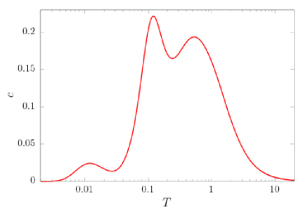
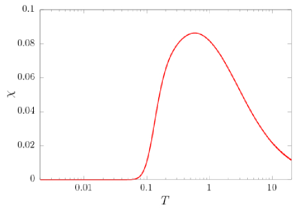
Figure 2: FTLM data ($R=100$) for the temperature dependence (logarithmic scale) of (top) the specific heat per site $c(T)$ and (bottom) the static uniform susceptibility per site $\chi(T)$ of the PHAF of $N=32$ sites.

The FTLM is the adequate approach to study the finite $S=1/2$ PHAF of $N=32$ sites. In Fig. 2 we show data for $c(T)$ (top) and $\chi(T)$ (bottom) over a wide temperature range using a logarithmic $T$ scale. The specific heat exhibits the typical main maximum at $T=0.53$ and, in addition, two low-$T$ maxima at $T=0.012$ and at $T=0.117$. While the maximum at $T=0.012$ is certainly a finite-size effect, one can speculate that the other low-$T$ maximum at $T=0.117$ signals an extra low-energy scale set by low-lying singlets (see the density of states shown in the inset of the middle panel of Fig. 3) that might be also relevant for the infinite system. Such a feature has been observed in low-dimensional highly frustrated quantum magnets, e.g., the spin-half kagome Heisenberg antiferromagnet (HAF), where the existence of such an extra low-$T$ peak is a subject of a long-standing and ongoing debate Elstner and Young (1994); Nakamura and Miyashita (1995); Tomczak and Richter (1996); Misguich and Bernu (2005); Munehisa (2014); Shimokawa and Kawamura (2016); Chen et al. (2018); Schnack et al. (2018). However, in the three-dimensional PHAF the finite-size effects are undoubtedly stronger than in the two-dimensional kagome HAF. Thus, to conclude a double-peak structure in $c(T)$ from our FTLM data is inappropriate. For the static uniform susceptibility $\chi(T)$ the low-lying singlets are not relevant and $\chi(T)$ does not show extra-peaks except the well-pronounced maximum that is typical for finite spin systems with $\chi_{0}\equiv\chi(T=0)=0$. Again, this behavior might be not representative for the infinite system, particularly, in case that $\chi_{0}>0$ for $N\to\infty$.

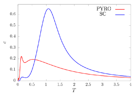
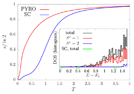
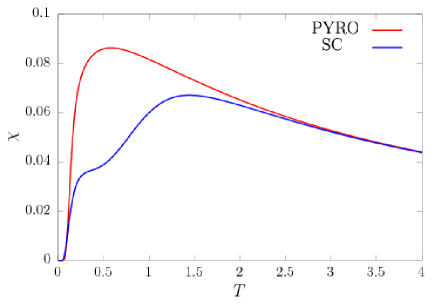
Figure 3: Comparison of FTLM data ($R=100$) of the PHAF of $N=32$ sites with corresponding ones of the simple-cubic HAF of $N=32$ sites. (Top) Specific heat per site $c(T)$. (Middle) Entropy per site $s(T)$. (Bottom) Static uniform susceptibility per site $\chi(T)$. The inset in the middle panel shows the histogram low-energy density of states (arbitrary units). Note that for the simple-cubic HAF there are only three tiny bars in the energy region shown here (their positions are indicated by green labels “sc”).

To quantify the temperature region where the finite $N=32$ lattice may be representative for the infinite lattice we compare in Figs. 4 and 5 several Padé approximants of the HTE series of the finite and the infinite lattices. Obviously, the data for $N=32$ and $N=\infty$ coincide only down to $T\sim 0.7$, thus, indicating that finite pyrochlore lattices accessible by FTLM are not suitable to discuss the thermodynamics of the spin-half PHAF below this temperature.

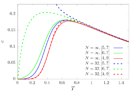
Figure 4: Several Padé approximants of the specific heat $c(T)$ of the PHAF: Comparison of the finite lattice of $N=32$ (broken) with the infinite lattice (solid).

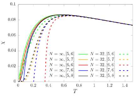
Figure 5: Several Padé approximants of the uniform susceptibility $\chi(T)$ of the PHAF: Comparison of the finite lattice of $N=32$ (broken) with the infinite lattice (solid).

Nevertheless, the finite-size data for the PHAF are useful to demonstrate frustration effects. For that we may compare the PHAF with the $S=1/2$ HAF on the simple-cubic lattice, because both have six nearest-neighbors, i.e., a simple mean-field decoupling of the Heisenberg Hamiltonian would yield identical thermodynamics. However, the simple-cubic HAF exhibits a finite-temperature phase transition to Néel order, but the PHAF does not order. Thus, we compare both models on finite lattices of $N=32$ sites, where the simple-cubic finite-temperature phase transition is irrelevant, see Fig. 3, where we compare FTLM data of the specific heat, the entropy, and the susceptibility using a linear $T$ scale for $N=32$. The tremendous influence of frustration is visible at all temperature scales. In particular, the spectrum at low energies in the frustrated system is much denser than that of the unfrustrated one [see the density of states (histogram, $\Delta E=0.02$) in the inset in the middle panel of Fig. 3], thus leading to the drastic differences at low $T$, see the upper and middle panels of Fig. 3. Remarkably, the noticeable differences in all quantities are present at pretty high temperatures. Only, beyond $T\gtrsim 3$ the corresponding curves approach each other. A striking effect of frustration is also the shift of the maximum in $\chi(T)$ to lower temperatures, see the lower panel of Fig. 3.

IV.2 Infinite lattice

Let us now move to a detailed investigation of the infinite PHAF by using the EM interpolation scheme, see Sec. III.1. Using our Magdeburg HTE code Schmidt et al. (2011); Lohmann (2012); Lohmann et al. (2014) we have created the HTE series for $c(T)$ and $\chi(T)$ up to order 13 (see Appendix B) that provides the high-temperature input for the EM. Since the EM finally uses Padé approximants of a power series of $s(e)$ derived from the initial HTE series, the HTE input determines the highest order of the Padé approximants of the EM interpolation scheme.

As a low-temperature input for the EM we need the ground-state energy $e_{0}$. There is a large variety of reported values for $e_{0}$ of the spin-half PHAF ranging from $e_{0}=-0.57$ to $e_{0}=-0.45$, namely, $e_{0}=-0.572$ Sobral and Lacroix (1997), $-0.56$ Canals and Lacroix (2000), $-0.49$ Harris et al. (1991); Koga and Kawakami (2001), $-0.482081$ Chandra and Sahoo (2018), $-0.466971$ Chandra and Sahoo (2018), $-0.459$ Kim and Han (2008), $-0.457804$ Isoda and Mori (1998), $-0.45093$ Müller et al. (2019), $-0.4473$ Burnell et al. (2009), i.e., accurate values for $e_{0}$ are missing. We also need the low-temperature law for $c(T)$, where we have to distinguish between gapped and gapless behavior (cf. Sec. III.1). Finally, in case of gapless excitations the exponent $\alpha$ of the power law is an input parameter, and for the susceptibility $\chi_{0}\equiv\chi(T=0)$ is required as input. Fortunately, for gapped excitations the value of the gap is not needed as an input, it is rather an output of the EM. Moreover, we have $\chi_{0}\equiv\chi(T=0)=0$ in this case.

We begin with the specific heat $c(T)$ for which the EM is better justified (two sum rules are exploited). Actually, the low-temperature law for $c(T)$ is not known for the $S=1/2$ PHAF. Advantageously, the previous ample of experience with the EM Bernu and Misguich (2001); Misguich and Bernu (2005); Bernu et al. (2013); Bernu and Lhuillier (2015); Schmidt et al. (2017); Bernu et al. (2019) provides valuable hints to overcome this difficulty. Thus, in case that these input data are too far from the true (but possibly unknown) data one gets inconsistent or unphysical results. Hence, to get physical (i.e., pole free) Padé approximants requires reasonable values for $e_{0}$ and reasonable assumptions on the low-$T$ behavior of $c(T)$. Moreover, getting a large number $n_{\rm P}$ of similar Padé approximants for a certain input data set indicates the physical relevance of this set. On the other hand, the appearance of significant differences between the various Padé approximants is a criterion to discard the corresponding input set. The successfulness of this strategy has been demonstrated for several examples where excellent reference data are available, in particular, for the $S=1/2$ $XY$, HAF, and Ising chains Bernu and Misguich (2001); Bernu and Lhuillier (2015), for the $S=1$ HAF (Haldane) chain Bernu and Misguich (2001), for the $S=1/2$ square-lattice and triangular-lattice Heisenberg ferro- and antiferromagnets Bernu and Misguich (2001) or for the $S=1/2$ kagome-lattice HAFs Misguich and Bernu (2005); Bernu and Lhuillier (2015); Bernu et al. (2019).

By combining different assumptions on the ground-state energy and low-$T$ behavior of $c(T)$ of the PHAF we have generated a large set of temperature profiles for the specific heat. In the next step, we use the guidelines described above to evaluate the used input data, this way obtaining definite conclusions on their relevance. In sum, a crucial criterion is that a particular input data set leads to a close bundle of temperature profiles obtained by many physical Padé approximants. Since, the high-temperature part is per se identical this criterion concerns the temperature region $T\lesssim 0.5$. In what follows, we will present in the main text only data for the most relevant input sets, whereas presentation of some other illustrative results, only briefly mentioned in the main text, are transferred to Appendix C.

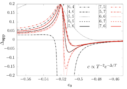
Figure 6: EM for gapped spectrum: The gap $\Delta_{\rm app}$ as it follows from Eq. (3.12) versus the ground-state energy $e_{0}$ varied in region $-0.57\ldots-0.45$.

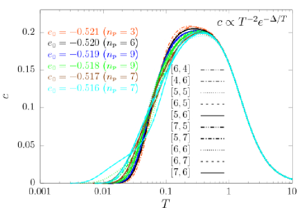
Figure 7: EM results for the specific heat; gapped spectrum, $e_{0}=-0.521\ldots-0.516$. The parameter $n_{\rm P}$ in brackets behind energy values denotes the number of (very similar) Padé approximants shown here.

As a first result, we found that the assumption of gapped excitations is not favorable for the following reasons. We varied $e_{0}$ in the region $-0.57\ldots-0.45$ and calculated the gap given in Eq. (3.12) using different Padé approximants, where we focused on nearly diagonal Padé approximants $[u,d](e)$, $u\sim d$, constructed from HTE data of 10th, 11th, 12th, and 13th order, see Fig. 6. We find that the gap $\Delta_{\rm app}$, Eq. (3.12), is negative if the ground-state energy exceeds approximately $-0.515$, thus providing evidence that a gapped spectrum together with $e_{0}\gtrsim-0.515$ can be excluded. For ground-state energies in the region $-0.519\ldots-0.517$ we obtain $\Delta_{\rm app}=0.16\ldots 0.18$, see Fig. 6 (and Fig. 16 in Appendix C), and there is a decent number $n_{\rm P}$ of Padé approximants yielding similar $c(T)$ profiles, see Fig. 7. For $e_{0}$ less than $-0.521$ the number of physical Padé approximants noticeably decreases. Although the results for $c(T$) do not entirely discard a gapped ground state, further EM analysis of $\chi(T)$ under this assumption leads to disagreement with diagrammatic Monte Carlo simulations of Ref. Huang et al. (2016) at $T<0.7$, see Fig. 13 below. We may consider these findings for $c(T$) and $\chi(T)$ as an indication to favor a gapless ground state. We mention that the Green’s function results indicate gapless magnetic excitations Müller et al. (2019), and, as mentioned already above, the data for $\chi(T)$ given in Huang et al. (2016) down to $T=J/6$ seem also to be in favor of gapless excitations.

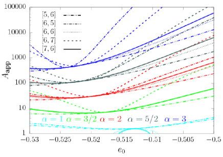
Figure 8: EM for gapless spectrum: The prefactor $A_{\rm app}$ as it follows from Eq. (3.8) for $\alpha=1,3/2,2,5/2,3$ versus the ground-state energy $e_{0}$ varied in the region $-0.53\ldots-0.50$.

We focus now on the gapless case with a power-law decay of the specific heat $c(T)=AT^{\alpha}$ as $T\to 0$. Since we do not know the exponent $\alpha$, we study different values $\alpha=1,3/2,2,5/2,3$. As for the gapped case, we again varied $e_{0}$ in the region $-0.57\ldots-0.45$. We observed that only in a much smaller region around $e_{0}=-0.52$ reasonable results can be obtained (see also the discussion of Fig. 8, below). Thus, in what follows we consider preferably the region $-0.53\ldots-0.50$ in more detail.

First we consider the prefactor $A_{\rm app}$ that is given within the EM by Eq. (3.8). According to above outlined criteria for physically relevant EM outcomes the values of $A_{\rm app}$ obtained by different Padé approximants must be very close to each other. From Fig. 8 (see also Fig. 17 in Appendix C for additional information) it is evident that for each value of $\alpha$ there is a well-defined relevant region of $e_{0}$, namely, $-0.515\ldots-0.513$ for $\alpha=1$, $-0.518\ldots-0.516$ for $\alpha=3/2$, $-0.521\ldots-0.518$ for $\alpha=2$, $-0.522\ldots-0.520$ for $\alpha=5/2$, $-0.524\ldots-0.522$ for $\alpha=3$. In all cases the ground-state energy is within the interval $e_{0}=-0.524\ldots-0.513$, which is much narrower than the wide region reported in the literature ranging from $e_{0}=-0.57$ to $e_{0}=-0.45$ Sobral and Lacroix (1997); Canals and Lacroix (2000); Harris et al. (1991); Koga and Kawakami (2001); Chandra and Sahoo (2018); Kim and Han (2008); Isoda and Mori (1998); Müller et al. (2019); Burnell et al. (2009).

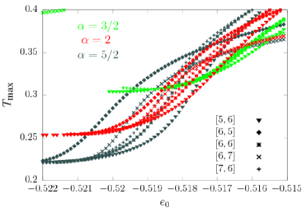
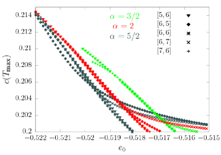
Figure 9: EM for gapless spectrum: Position $T_{\max}$ (top) and height $c(T_{\max})$ (bottom) of the specific heat versus the ground-state energy $e_{0}$ varied in the region region $-0.522\ldots-0.515$ for exponents $\alpha=3/2$ (green), $\alpha=2$ (red), and $\alpha=5/2$ (dark gray).

We consider the coincidence of $A$ values for different Padé approximants as a necessary criterion to figure out regions of relevant values for $e_{0}$ and $\alpha$. Since $A$ (together with $\alpha$) determines the $c(T)$ profile at sufficiently low $T$, we can get additional reliability by examining the region around the main (“high”-temperature) maximum. For that we compare the position $T_{\max}$ and the height $c(T_{\max})$ of this maximum obtained from different Padé approximants in dependence on $e_{0}$ within the regions guided by the previous inspection of $A$ for $\alpha=3/2,2,5/2$ in Fig. 9 (Fig. 18 in Appendix C reports such data for a wider region of $e_{0}$ including also $\alpha=1$ and $3$). For each $\alpha$ we find pretty small regions of $e_{0}$ which yield almost identical $T_{\max}$ and $c(T_{\max})$, and, consistently, this region fits well to the region obtained by inspection of $A$. For example, for $\alpha=2$ all Padé approximants give almost identical $T_{\max}$ and $c(T_{\max})$, cf. Fig. 9 (red symbols), if $e_{0}$ is taken within the region $-0.522\ldots-0.519$, which is in excellent agreement with that obtained from the prefactor $A$, see above. Note, however, that for $\alpha=1$ and $3$ the diversity of $T_{\max}$ and $c(T_{\max})$ is noticeably larger than for $\alpha=3/2,2,5/2$, cf. Fig. 18 in Appendix C, indicating that the exponents $\alpha=1$ and $3$ are less favorable.

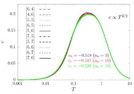
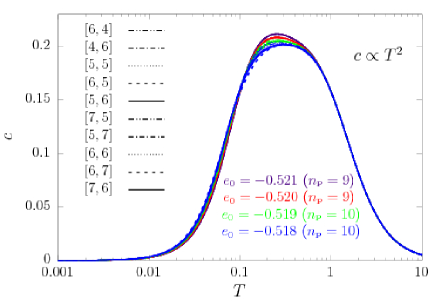
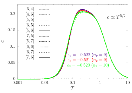
Figure 10: EM results for the specific heat; gapless spectrum. (Top) $e_{0}=-0.518\ldots-0.516$, $\alpha=3/2$. (Middle) $e_{0}=-0.521\ldots-0.518$, $\alpha=2$. (Bottom) $e_{0}=-0.522\ldots-0.520$, $\alpha=5/2$. The parameter $n_{\rm P}$ in brackets behind energy values denotes the number of (very similar) Padé approximants shown here.

Finally, after the specification of the ground-state energy values as outlined above, we present in Fig. 10 the full $c(T)$ curves obtained by the EM for $\alpha=3/2,2,5/2$ and a few related optimal values of $e_{0}$. [Corresponding curves for $\alpha=1$ and $\alpha=3$ are shown in Fig. 19 in Appendix C. Moreover, Fig. 20 in Appendix C provides additional results of $c(T)$ comparing data for all $\alpha=1,3/2,2,5/2,3$ for various values of $e_{0}$.]

As can be seen in Fig. 10, there is a quite large number of Padé approximants (see the parameter $n_{\rm P}$ in brackets behind energy values) yielding very similar temperature profiles $c(T)$. Thus, for $\alpha=2$ we show in the middle panel of Fig. 10 $n_{\rm P}=10$ Padé approximants if $e_{0}=-0.519$ and $-0.518$ and $n_{\rm P}=9$ Padé approximants if $e_{0}=-0.521$ and $e_{0}=-0.520$. Outside this region of $e_{0}$ values the number of physical Padé approximants becomes noticeably smaller.

Without favoring any of the assumptions on the low-$T$ behavior of $c(T)$ and taking into account all (i.e., gapped and gapless excitations) EM predictions for $c(T)$ collected in Figs. 7 and 10 (see also Fig. 21 in Appendix C, where we present a direct comparison of both cases), we have clear evidence 1) for a quite narrow region of reasonable $e_{0}$ values and 2) for the absence of a double-peak profile in $c(T)$. 3) Though, the position $T_{\max}$ and the height $c(T_{\max})$ of the maximum of the specific heat slightly depend on the assumption about the ground-state energy $e_{0}$ and low-lying excitations, all cases yield $T_{\max}$ around $\approx 0.25$ and $c(T_{\max})$ around $\approx 0.2$.

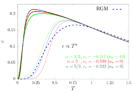
Figure 11: Specific heat $c(T)$ of the $S=1/2$ PHAF: Comparison of our EM data ($e_{0}=-0.522$, $\alpha=5/2$; $e_{0}=-0.520$, $\alpha=2$; $e_{0}=-0.517$, $\alpha=3/2$) with results obtained by the rotation-invariant Green’s function method Müller et al. (2019) (dashed blue) and by the HTE (thin solid curves; we show the same HTE data for $N=\infty$ as shown in Fig. 4).

Finally, we compare our EM results for $c(T$) with data calculated by HTE (without subsequent EM interpolation) and by the Green’s function approach Müller et al. (2019), cf. Fig. 11. The Green’s function results deviate from the EM results already below $T\sim 1$, whereas the HTE data deviate below $T\sim 0.7$.

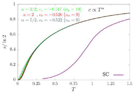
Figure 12: EM data for the entropy for the gapless case with $e_{0}=-0.522$, $\alpha=5/2$; $e_{0}=-0.520$, $\alpha=2$; $e_{0}=-0.517$, $\alpha=3/2$. We also show quantum Monte-Carlo data for the simple-cubic HAF Wessel (2010) as well as HTE data (thin solid lines), where we show the same Padé approximants as used in Fig. 4 for $c(T)$. (Note the the HTE data are very close to the EM data.)

The EM straightforwardly also provides the temperature profile of the entropy $s(T)$, see Fig. 12. Since the finite-temperature phase transition present in the simple-cubic HAF does not influence $s(T)$ as much as $c(T)$, we compare the data for the PHAF with corresponding ones for the simple-cubic HAF taken from Ref. Wessel (2010). We also show HTE data. Similar as already found for the finite system, cf. the middle panel of Fig. 3, the frustration leads to a much faster increase of $s$ at low temperatures for the PHAF. Thus, at $T=0.5$ the entropy already amounts to more than 50% of its maximal value $\ln 2\approx 0.69$. (Note that in Fig. 22 in Appendix C we present a direct comparison of the gapped and gapless temperature profiles of $s$.)

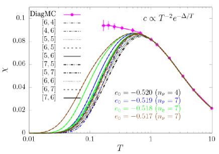
Figure 13: EM results for the susceptibility; gapped spectrum, $e_{0}=-0.520\ldots-0.517$.

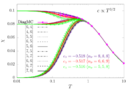
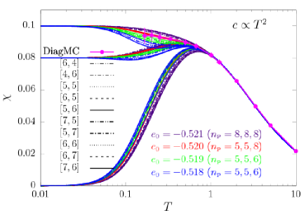
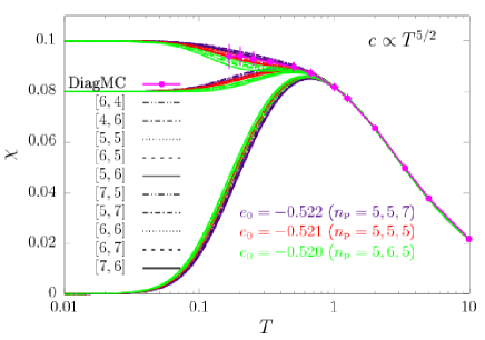
Figure 14: EM results for the susceptibility; gapless spectrum. (Top) $e_{0}=-0.518\ldots-0.516$, $\alpha=3/2$. (Middle) $e_{0}=-0.521\ldots-0.518$, $\alpha=2$. (Bottom) $e_{0}=-0.522\ldots-0.520$, $\alpha=5/2$. $\chi_{0}=0,0.08,0.1$. Three values of $n_{\rm P}$ in brackets correspond to the assumed values $\chi_{0}=0.1$, $\chi_{0}=0.08$, and $\chi_{0}=0$, consequently.

We consider now the static uniform susceptibility $\chi$ calculated by the EM as described in Sec. III.1. According to the results of the rotation-invariant Green’s function method, there is $\chi_{0}\equiv\chi(T=0)>0$. A non-zero $\chi_{0}$ may be also expected from the diagrammatic Monte Carlo simulations Huang et al. (2016). Nevertheless, we will not exclude from the beginning $\chi_{0}=0$, i.e., a non-zero spin gap. Although the above discussed EM data for $c(T)$ are in favor of a gapless spectrum, the specific heat profiles were not fully conclusive to entirely reject the gapped spectrum. Moreover, one could have gapless singlet (i.e., non-magnetic) excitations but gapped triplet (i.e., magnetic) excitations. Thus we studied the case with exponential decay of $\chi(T)$ and $c(T)$ as $T\to 0$ (i.e., gapped singlet and triplet excitations), see Fig. 13, as well as the case with exponential decay of $\chi(T)$ and power-law decay of $c(T)$ as $T\to 0$, (i.e., gapless singlet and gapped triplet excitations), see Fig. 14, where we consider those values for $e_{0}$ and $\alpha$ which are previously used to get $c(T)$ (see also Figs. 23 and 24 in Appendix C). From these figures, it is obvious that the susceptibility profiles based on gapped magnetic excitations are not compatible with the diagrammatic Monte Carlo data of Ref. Huang et al. (2016) in the temperature region below $0.7$, thus providing further evidence against a gapped spectrum. On the other hand, the EM results for gapless excitations with $\alpha=3/2,2,5/2$ and $e_{0}=-0.522\ldots-0.516$ and with non-zero $\chi_{0}$ as shown in Fig. 14 fit much better to the data of Ref. Huang et al. (2016).

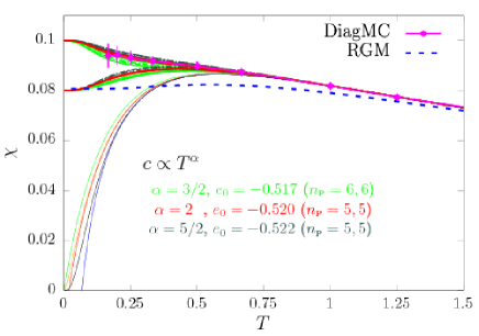
Figure 15: Susceptibility $\chi(T)$ of the $S=1/2$ PHAF: Comparison of our EM data ($e_{0}=-0.522$, $\alpha=5/2$; $e_{0}=-0.520$, $\alpha=2$; $e_{0}=-0.517$, $\alpha=3/2$) with results obtained by the rotation-invariant Green’s function method Müller et al. (2019) (dashed blue), by diagrammatic Monte Carlo Huang et al. (2016), and by the HTE (thin solid curves; we show the same HTE data for $N=\infty$ as shown in Fig. 5).

As for the specific heat, we finally compare our EM results for $\chi(T$) with data calculated by HTE (without subsequent EM interpolation), by the Green’s function approach Müller et al. (2019), cf. Fig. 15, where we also include the data of the diagrammatic Monte Carlo simulations Huang et al. (2016). The Green’s function results deviate already below $T\sim 1.5$, and the HTE coincides down to $T\sim 0.7$, whereas $\chi(T)$ profiles with $\chi_{0}=0.1$ are in excellent agreement with the data of Ref. Huang et al. (2016).

V Conclusions and summary

We have studied the specific heat $c(T)$, the entropy $s(T)$, and the static uniform susceptibility $\chi(T)$ of the spin-half pyrochlore Heisenberg antiferromagnet (PHAF) on a finite lattice of $N=32$ sites using the finite-temperature Lanczos method (FTLM) and on the infinite lattice using the high-temperature expansion (HTE) up to order 13 and a sophisticated interpolation between the low- and high-temperature behavior of the thermodynamic potential entropy $s$ as a function of internal energy $e$ [the entropy method (EM)].

We found that finite lattices of such size are not appropriate to get reasonable results below $T\sim 0.7$, but they might be useful to get a general impression on the strong frustration effects present in the PHAF by comparison of the HAF on finite pyrochlore and simple-cubic lattices. A similar limitation to temperatures above $T\sim 0.7$ is valid for the HTE even if the range of validity of the high-temperature series is extended by Padé approximants. Only the EM interpolation is suitable to overcome these limitation and to provide sound data for the whole temperature range.

Our main findings for the specific heat $c(T)$ are as follows. (i) Contrary to the two-dimensional kagome HAF, we do not find hints neither for an extra low-$T$ peak nor an extra shoulder below the main maximum. However, the absence of an extra low-$T$ feature goes hand in hand with a significant shift of the single maximum towards $T\sim 0.25$, which is much lower than for the kagome HAF, where the main maximum is at $T_{\rm max}/J=0.67$ Schnack et al. (2018); Bernu et al. (2019). This conclusion is robust, i.e., it is obtained not only for gapless excitations for all reasonable exponents $\alpha$ of the low-temperature power law of $c(T)$, but holds also for gapped excitations. (ii) A gapless spectrum is more favorable than a gapped one, i.e., most likely there is power-law low-$T$ behavior of $c(T)$. Although best results are for an exponent $\alpha=2$, other exponents ($\alpha=1,3/2,5/2,3$) cannot be excluded. (iii) We predict a ground-state energy $e_{0}\approx-0.52$ .

Our EM data for the susceptibility $\chi(T)$ in comparison with data obtained by diagrammatic Monte Carlo Huang et al. (2016) provide further evidence for a gapless spectrum with a ground-state energy $e_{0}\approx-0.52$. The temperature profile of $\chi$ most likely does not show a maximum, rather there is a monotonous increase of $\chi$ upon decreasing of $T$ reaching a zero-temperature value of $\chi_{0}\approx 0.1$.

Recently, we have learned that R. Schäfer et al. et al. (2020) also examined thermodynamics of the quantum PHAF, however, using for that numerical linked-cluster expansions.

Appendix A: M. Planck’s derivation of the specific heat $c(T)$ of an oscillator

In his revolutionary paper in 1900 Planck (1900) (see also the Nobel Prize address [Notes 7, 12, and 13 at the end of the Nobel Prize address “The origin and development of the quantum theory” by Max Planck delivered before the Royal Swedish Academy of Sciences at Stockholm, 2 June, 1920] Planck (The Clarendon Press, Oxford 1922)), M. Planck investigated the energy distribution of electromagnetic radiation emitted by a black body in thermal equilibrium. For that he considered the entropy of the equilibrium radiation $S$ in relation with its energy $U$, or more accurately, the second derivative ${\rm d}^{2}S/{\rm d}U^{2}$. According to Wien’s law it is

$$\frac{{\rm d}^{2}S}{{\rm d}U^{2}}=-\frac{1}{bU}.$$ (A.1)

But in view of experiments for high temperatures one has $U=cT$, i.e.,

$$\frac{{\rm d}^{2}S}{{\rm d}U^{2}}=-\frac{c}{U^{2}}.$$ (A.2)

(M. Planck here refers to experiments by F. Kurlbaum.) While Wien’s law (A.1) is valid for small energy values (short wave length), Eq. (A.2) describes the high-energy limit (long wave length, Rayleigh-Jeans law). To get agreement with experimental data M. Planck suggested

$$\frac{{\rm d}^{2}S}{{\rm d}U^{2}}=-\frac{c}{U\left(bc+U\right)}\longrightarrow\left\{\begin{array}[]{cc}-\frac{1}{bU},&U\ll bc,\\ -\frac{c}{U^{2}},&U\gg bc,\end{array}\right.$$ (A.5)

which interpolates between both limiting cases. By integrating we get

$$\frac{1}{T}=\frac{{\rm d}S}{{\rm d}U}=\frac{1}{b}\ln\left(1+\frac{bc}{U}\right),$$ (A.6)

which yields Planck’s formula

$$U=\frac{bc}{e^{b/T}-1}.$$ (A.7)

These arguments can be formulated within the setup of the entropy method to find the specific heat $c(T)$ of a (Bose) oscillator, which represents the electromagnetic radiation with the frequency $\nu=2\pi\omega$. Now we know that $b=\hbar\omega$ and $c=1$. Taking into account the zero-point energy we have to replace $U\to e=U+\hbar\omega/2$. Then the Planck’s interpolation formula (A.5) for the auxiliary function $G(e)=(s(e))^{\prime\prime}$ reads:

$$G(e)=-\frac{1}{\left(e-\frac{\hbar\omega}{2}\right)\left(e+\frac{\hbar\omega}{2}\right)}=\frac{1}{\left(\frac{\hbar\omega}{2}\right)^{2}-e^{2}}$$

$$\longrightarrow\left\{\begin{array}[]{cc}-\frac{1}{\hbar\omega\left(e-\frac{\hbar\omega}{2}\right)},&e\ll\hbar\omega,\\ -\frac{1}{e^{2}},&e\gg\hbar\omega.\end{array}\right.$$ (A.10)

The subscript app in the left-hand side of this equation is omitted since the suggested expression for $G(e)=(s(e))^{\prime\prime}$ (Appendix A: M. Planck’s derivation of the specific heat $c(T)$ of an oscillator) appears to be exact. By integrating we get

$$\frac{1}{T}=s^{\prime}(e)=\int\limits_{e}^{\infty}{\rm d}e\frac{1}{e^{2}-\left(\frac{\hbar\omega}{2}\right)^{2}}=\frac{1}{\frac{\hbar\omega}{2}}{\rm arccth}\frac{e}{\frac{\hbar\omega}{2}}$$ (A.11)

and then

$$c(e)=-\frac{(s^{\prime}(e))^{2}}{s^{\prime\prime}(e)}=\frac{e^{2}-\left(\frac{\hbar\omega}{2}\right)^{2}}{\left(\frac{\hbar\omega}{2}\right)^{2}}{\rm arccth}^{2}\frac{e}{\frac{\hbar\omega}{2}}$$ (A.12)

and finally

$$c(T)=\left(\frac{\frac{\hbar\omega}{2T}}{{\rm sh}\frac{\hbar\omega}{2T}}\right)^{2}.$$ (A.13)

Appendix B: HTE for the $S=1/2$ PHAF

We report here the HTE coefficients for the spin-half PHAF up to order 13 obtained by the Magdeburg HTE code developed mainly by A. Lohmann Lohmann (2012). Note that the coefficients up to order 10 where presented previously for arbitrary spin $S$ in Refs. Schmidt et al. (2011); Lohmann et al. (2014).

For the specific heat (per site) we have

$$c(\beta)=\sum_{i}d_{i}\beta^{i},$$

$$d_{1}=0,\;\frac{d_{2}}{J^{2}}=+\frac{9}{16},\;\frac{d_{3}}{J^{3}}=-\frac{9}{32},\;\frac{d_{4}}{J^{4}}=-\frac{207}{256},$$

$$\frac{d_{5}}{J^{5}}=+\frac{195}{256},\;\frac{d_{6}}{J^{6}}=+\frac{3\,549}{4\,096},$$

$$\frac{d_{7}}{J^{7}}=-\frac{59\,073}{40\,960},\;\frac{d_{8}}{J^{8}}=-\frac{34\,535}{65\,536},$$

$$\frac{d_{9}}{J^{9}}=+\frac{345\,491}{163\,840},\;\frac{d_{10}}{J^{10}}=-\frac{9\,385\,203}{36\,700\,160},$$

$$\frac{d_{11}}{J^{11}}=-\frac{337\,285\,883}{132\,120\,576},\;\frac{d_{12}}{J^{12}}=+\frac{39\,036\,781\,051}{26\,424\,115\,200},$$

$$\frac{d_{13}}{J^{13}}=+\frac{144\,963\,365\,443}{58\,133\,053\,440}.\quad$$ (B.1)

For the static uniform susceptibility (per site) we have

$$\chi(\beta)=\sum_{i}c_{i}\beta^{i},$$

$$c_{1}=+\frac{1}{4},\;\frac{c_{2}}{J}=-\frac{3}{8},\;\frac{c_{3}}{J^{2}}=+\frac{3}{8},\;\frac{c_{4}}{J^{3}}=-\frac{17}{64},$$

$$\frac{c_{5}}{J^{4}}=+\frac{85}{512},\;\frac{c_{6}}{J^{5}}=-\frac{97}{640},$$

$$\frac{c_{7}}{J^{6}}=+\frac{20\,207}{122\,880},\;\frac{c_{8}}{J^{7}}=-\frac{210\,989}{1\,720\,320},$$

$$\frac{c_{9}}{J^{8}}=+\frac{92\,147}{1\,966\,080},\;\frac{c_{10}}{J^{9}}=-\frac{4\,936\,709}{247\,726\,080},$$

$$\frac{c_{11}}{J^{10}}=+\frac{540\,939\,383}{9\,909\,043\,200},\;\frac{c_{12}}{J^{11}}=-\frac{5\,315\,724\,257}{72\,666\,316\,800},$$

$$\frac{c_{13}}{J^{12}}=+\frac{20\,479\,483\,351}{747\,424\,972\,800}.\quad$$ (B.2)

Appendix C: Additional EM data for $c$, $s$, and $\chi$ of the $S=1/2$ PHAF

In this appendix we collect more figures presenting EM data for the specific heat, the entropy, and the susceptibility which are briefly discussed but not shown as figures in Sec. IV.2.

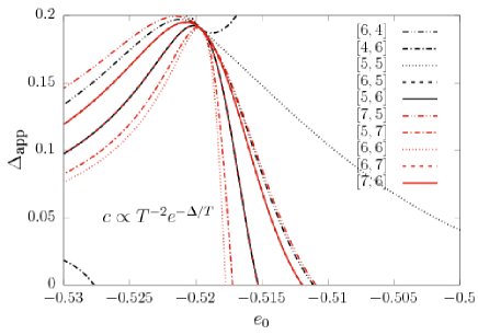
Figure 16: The same as in Fig. 6, but for $e_{0}$ values within a narrower region $-0.53\ldots-0.50$.

In Fig. 16 we show some results related to Fig. 6 using a smaller region of $e_{0}$.

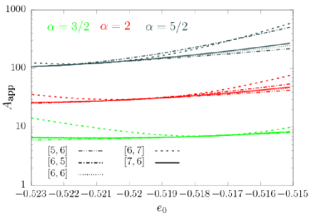
Figure 17: The same as in Fig. 8, but for $\alpha=3/2,2,5/2$ only and a narrower region of $e_{0}=-0.523\ldots-0.515$.

In Fig. 17 we show some results related to Fig. 8 using a smaller region of $e_{0}$. The region of $e_{0}$ in which various Padé approximants yield almost the same prefactor $A_{\rm app}$ (3.8) is different for $\alpha=3/2,2,5/2$. Clearly, the values of $\alpha$ and $A$ are linked. For example, after assuming $\alpha=2$ for $e_{0}=-0.520\ldots-0.519$ the EM prediction for the specific heat as $T\to 0$ reads: $c(T)=A_{\rm app}T^{2}$ with $A_{\rm app}=29\ldots 31$.

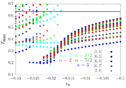
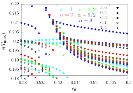
Figure 18: The same as in Fig. 9, but for wider region of $e_{0}=-0.53\ldots-0.5$ and all five values of $\alpha=1,3/2,2,5/2,3$. Black straight lines correspond to the Padé approximant $[6,7]$ of high-temperature series of $c(T)$ [$T_{\max}\approx 0.637$, $c(T_{\max})\approx 0.182$].

In Fig. 18 we show some results related to Fig. 9 using a wider region of $e_{0}$ and including exponents $\alpha=1$ and $\alpha=3$. The position and the height of the maximum of the specific heat, as they follow from raw HTE series extended by the Padé approximant $[6,7]$, have the values $T_{\max}\approx 0.637$ and $c(T_{\max})\approx 0.182$. The EM predictions for $\alpha=2$ and $e_{0}=-0.520\ldots-0.519$ are different: $T_{\max}\approx 0.25\ldots 0.28$ and $c(T_{\max})\approx 0.205\ldots 0.208$.

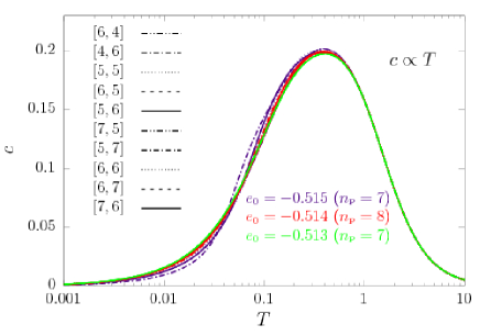
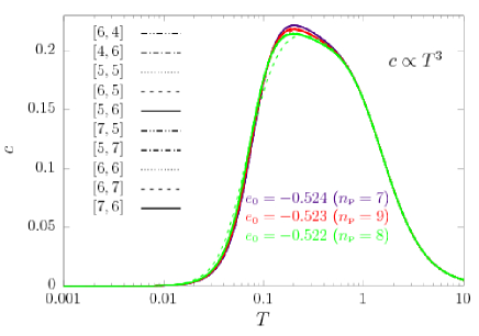
Figure 19: Supplement to Fig. 10; EM results for the specific heat; gapless spectrum. (Top) $e_{0}=-0.515\ldots-0.513$, $\alpha=1$. (Bottom) $e_{0}=-0.524\ldots-0.522$, $\alpha=3$.

Fig. 19 is supplementary to Fig. 10 of the main text. It contains similar EM predictions for $c(T)$ under less favorable assumptions $\alpha=1$ and $\alpha=3$.

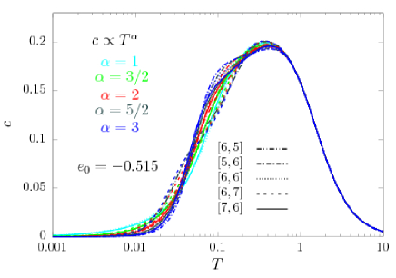
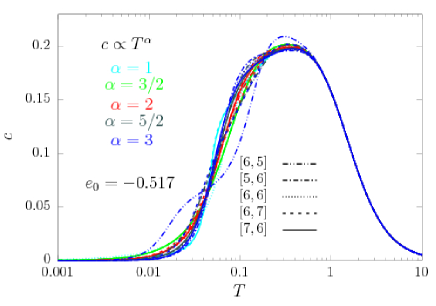
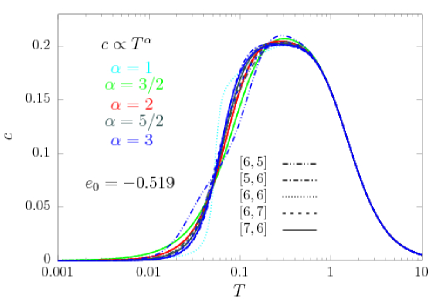
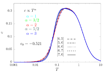
Figure 20: EM results for the specific heat; gapless spectrum. Various $e_{0}=-0.521\ldots-0.515$ (from bottom to top) and $\alpha=1,3/2,2,5/2,3$ (cyan, green, red, magenta, blue, respectively).

Fig. 20 provides temperature profiles of the specific heat which complement those shown in Fig. 10 and Fig. 19: We show $c(T)$ for $e_{0}=-0.521$, $e_{0}=-0.519$, $e_{0}=-0.517$, and $e_{0}=-0.515$ (from bottom to top) and compare data for $\alpha=1$ (cyan), $\alpha=3/2$ (green), $\alpha=2$ (red), $\alpha=5/2$ (magenta), and $\alpha=3$ (blue). The shown temperature profiles allow to estimate how close to each other are the various EM data based on different Padé approximants.

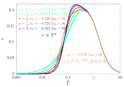
Figure 21: Specific heat $c(T)$ of the $S=1/2$ PHAF: Comparison of EM data for gapped (light brown) and gapless (other colors) excitations.

In Fig. 21 we collect the best (i.e., for such a value of $e_{0}$ which gives the largest number of almost coinciding resulting curves) EM predictions for $c(T)$ for the gapped and the gapless spectrum.

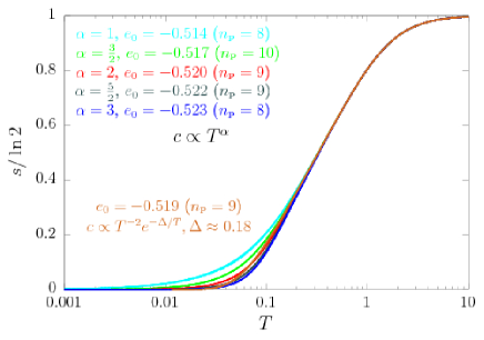
Figure 22: Comparison of EM data for the entropy for the gapped and gapless cases.

The best EM results for the temperature dependence of the entropy are shown in Fig. 22. Note, all curves for each color are indistinguishable in this figure.

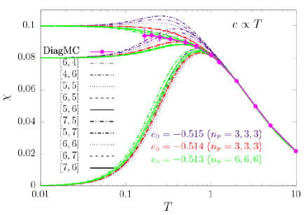
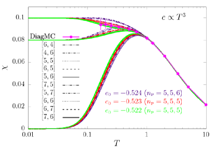
Figure 23: Supplement to Fig. 14; EM results for the susceptibility; gapless spectrum. (Top) $e_{0}=-0.515\ldots-0.513$, $\alpha=1$. (Bottom) $e_{0}=-0.524\ldots-0.522$, $\alpha=3$. $\chi_{0}=0,0.08,0.1$.

Fig. 23 is supplementary to Fig. 14 of the main text. It presents EM results for $\chi(T)$ for less favorable exponents $\alpha=1$ and $\alpha=3$.

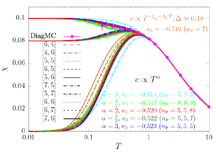
Figure 24: Susceptibility $\chi(T)$ of the $S=1/2$ PHAF: Comparison of EM data under the gapped (light brown) and gapless (other colors) assumptions. $\chi_{0}=0,0.08,0.1$.

In Fig. 24 we collect the best (i.e., for such a value of $e_{0}$ which gives the largest number of almost coinciding resulting curves) EM predictions for $\chi(T)$ under the gapped assumption and the gapless assumption with several values of $\alpha$. Note, $\chi(T)$ as it follows from the assumption about gapless singlet excitations but $\chi_{0}=0$ (all colors except light brown) deviates stronger from the diagrammatic Monte Carlo result than $\chi(T)$ as it follows from the assumption about gapped excitations (light brown). However, the agreement of different seven $\chi(T)$ curves for the latter case is rather poor.

References

- Gardner et al. (2010) J. S. Gardner, M. J. P. Gingras, and J. E. Greedan, “Magnetic pyrochlore oxides,” Rev. Mod. Phys. 82, 53 (2010).
- Gingras and McClarty (2014) M. J. P. Gingras and P. A. McClarty, “Quantum spin ice: a search for gapless quantum spin liquids in pyrochlore magnets,” Reports on Progress in Physics 77, 056501 (2014).
- Rau and Gingras (2019) Jeffrey G. Rau and Michel J.P. Gingras, “Frustrated quantum rare-earth pyrochlores,” Annual Review of Condensed Matter Physics 10, 357–386 (2019).
- Reimers et al. (1991) J. N. Reimers, A. J. Berlinsky, and A.-C. Shi, “Mean-field approach to magnetic ordering in highly frustrated pyrochlores,” Phys. Rev. B 43, 865 (1991).
- Reimers (1992) J. N. Reimers, “Absence of long-range order in a three-dimensional geometrically frustrated antiferromagnet,” Phys. Rev. B 45, 7287–7294 (1992).
- Moessner and Chalker (1998a) R. Moessner and J. T. Chalker, “Properties of a classical spin liquid: The Heisenberg pyrochlore antiferromagnet,” Phys. Rev. Lett. 80, 2929 (1998a).
- Moessner and Chalker (1998b) R. Moessner and J. T. Chalker, “Low-temperature properties of classical geometrically frustrated antiferromagnets,” Phys. Rev. B 58, 12049 (1998b).
- Isakov et al. (2004) S. V. Isakov, K. Gregor, R. Moessner, and L. Sondhi, “Dipolar spin correlations in classical pyrochlore magnets,” Phys. Rev. Lett. 93, 167204 (2004).
- Henley (2010) C. L. Henley, “The Coulomb phase in frustrated systems,” Annu. Rev. Condens. Matter Phys. 1, 179 (2010).
- Lapa and Henley (2012) M. F. Lapa and C. L. Henley, “Ground states of the classical antiferromagnet on the pyrochlore lattice,” arXiv:1210.6810 (2012).
- Iqbal et al. (2019) Y. Iqbal, T. Müller, P. Ghosh, M. J. P. Gingras, H. O. Jeschke, S. Rachel, J. Reuther, and R. Thomale, “Quantum and classical phases of the pyrochlore Heisenberg model with competing interactions,” Phys. Rev. X 9, 011005 (2019).
- Harris et al. (1991) A. B. Harris, A. J. Berlinsky, and C. Bruder, “Ordering by quantum fluctuations in a strongly frustrated Heisenberg antiferromagnet,” J. Appl. Phys. 69, 5200 (1991).
- Isoda and Mori (1998) M. Isoda and S. Mori, “Valence-bond crystal and anisotropic excitation spectrum on 3-dimensionally frustrated pyrochlore,” J. Phys. Soc. Jpn. 67, 4022 (1998).
- Canals and Lacroix (1998) B. Canals and C. Lacroix, “Pyrochlore antiferromagnet: A three-dimensional quantum spin liquid,” Phys. Rev. Lett. 80, 2933 (1998).
- Canals and Lacroix (2000) B. Canals and C. Lacroix, “Quantum spin liquid: The Heisenberg antiferromagnet on the three-dimensional pyrochlore lattice,” Phys. Rev. B 61, 1149 (2000).
- Koga and Kawakami (2001) A. Koga and N. Kawakami, “Frustrated Heisenberg antiferromagnet on the pyrochlore lattice,” Phys. Rev. B 63, 144432 (2001).
- Tsunetsugu (2001a) H. Tsunetsugu, “Antiferromagnetic quantum spins on the pyrochlore lattice,” J. Phys. Soc. Jpn. 70, 640 (2001a).
- Tsunetsugu (2001b) H. Tsunetsugu, “Spin-singlet order in a pyrochlore antiferromagnet,” Phys. Rev. B 65, 024415 (2001b).
- Berg et al. (2003) E. Berg, E. Altman, and A. Auerbach, “Singlet excitations in pyrochlore: A study of quantum frustration,” Phys. Rev. Lett. 90, 147204 (2003).
- Moessner et al. (2006) R. Moessner, S. L. Sondhi, and M. O. Goerbig, “Quantum dimer models and effective Hamiltonians on the pyrochlore lattice,” Phys. Rev. B 73, 094430 (2006).
- Tchernyshyov et al. (2006) O. Tchernyshyov, R. Moessner, and S. L. Sondhi, “Flux expulsion and greedy bosons: Frustrated magnets at large ,” Europhysics Letters (EPL) 73, 278–284 (2006).
- Kim and Han (2008) J. H. Kim and J. H. Han, “Chiral spin states in the pyrochlore Heisenberg magnet: Fermionic mean-field theory and variational Monte Carlo calculations,” Phys. Rev. B 78, 180410 (2008).
- Burnell et al. (2009) F. J. Burnell, Shoibal Chakravarty, and S. L. Sondhi, “Monopole flux state on the pyrochlore lattice,” Phys. Rev. B 79, 144432 (2009).
- Chandra and Sahoo (2018) V. R. Chandra and J. Sahoo, “Spin-1/2 Heisenberg antiferromagnet on the pyrochlore lattice: An exact diagonalization study,” Phys. Rev. B 97, 144407 (2018).
- Müller et al. (2019) Patrick Müller, Andre Lohmann, Johannes Richter, and Oleg Derzhko, “Thermodynamics of the pyrochlore-lattice quantum Heisenberg antiferromagnet,” Phys. Rev. B 100, 024424 (2019).
- Huang et al. (2016) Y. Huang, K. Chen, Y. Deng, N. Prokof’ev, and B. Svistunov, “Spin-ice state of the quantum Heisenberg antiferromagnet on the pyrochlore lattice,” Phys. Rev. Lett. 116, 177203 (2016).
- Schmidt et al. (2011) H.-J. Schmidt, A. Lohmann, and J. Richter, “Eighth-order high-temperature expansion for general Heisenberg Hamiltonians,” Phys. Rev. B , 104443 (2011).
- Planck (1900) Max Planck, “Über eine Verbesserung der Wienschen Spektralgleichung,” Verhandl. Dtsch. Phys. Ges. 2, 202–204 (1900).
- Bernu and Misguich (2001) B. Bernu and G. Misguich, “Specific heat and high-temperature series of lattice models: Interpolation scheme and examples on quantum spin systems in one and two dimensions,” Phys. Rev. B 63, 134409 (2001).
- Misguich and Bernu (2005) G. Misguich and B. Bernu, “Specific heat of the Heisenberg model on the kagome lattice: High-temperature series expansion analysis,” Phys. Rev. B 71, 014417 (2005).
- Plumb et al. (2019) K. W. Plumb, Hitesh J. Changlani, A. Scheie, Shu Zhang, J. W. Kriza, J. A. Rodriguez-Rivera, Yiming Qiu, B. Winn, R. J. Cava, and C. L. Broholm, “Continuum of quantum fluctuations in a three-dimensional Heisenberg magnet,” Nature Physics 15, 54 (2019).
- Zhang et al. (2019) Shu Zhang, Hitesh J. Changlani, Kemp W. Plumb, Oleg Tchernyshyov, and Roderich Moessner, “Dynamical structure factor of the three-dimensional quantum spin liquid candidate NaCaNi2F7,” Phys. Rev. Lett. 122, 167203 (2019).
- Greedan et al. (1986) J. E. Greedan, M. Sato, Xu Yan, and F. S. Razavi, “Spin-glass-like behavior in Y2Mo2O7, a concentrated, crystalline system with negligible apparent disorder,” Solid State Communications 59, 895 (1986).
- Silverstein et al. (2014) H. J. Silverstein, K. Fritsch, F. Flicker, A. M. Hallas, J. S. Gardner, Y. Qiu, G. Ehlers, A. T. Savici, Z. Yamani, K. A. Ross, B. D. Gaulin, M. J. P. Gingras, J. A. M. Paddison, K. Foyevtsova, R. Valenti, F. Hawthorne, C. R. Wiebe, and H. D. Zhou, “Liquidlike correlations in single-crystalline Y2Mo2O7: An unconventional spin glass,” Phys. Rev. B 89, 054433 (2014).
- Thygesen et al. (2017) P. M. M. Thygesen, J. A. M. Paddison, R. Zhang, K. A. Beyer, K. W. Chapman, H. Y. Playford, M. G. Tucker, D. A. Keen, M. A. Hayward, and A. L. Goodwin, “Orbital dimer model for the spin-glass state in Y2Mo2O7,” Phys. Rev. Lett. 118, 067201 (2017).
- Gao et al. (2018) S. Gao, K. Guratinder, U. Stuhr, J. S. White, M. Mansson, B. Roessli, T. Fennell, V. Tsurkan, A. Loidl, M. Ciomaga Hatnean, G. Balakrishnan, S. Raymond, L. Chapon, V. O. Garlea, A. T. Savici, A. Cervellino, A. Bombardi, D. Chernyshov, Ch. Rüegg, J. T. Haraldsen, and O. Zaharko, “Manifolds of magnetic ordered states and excitations in the almost Heisenberg pyrochlore antiferromagnet MgCr2O4,” Phys. Rev. B 97, 134430 (2018).
- Ji et al. (2009) S. Ji, S.-H. Lee, C. Broholm, T. Y. Koo, W. Ratcliff, S.-W. Cheong, and P. Zschack, “Spin-lattice order in frustrated ZnCr2O4,” Phys. Rev. Lett. 103, 037201 (2009).
- Matsuda et al. (2007) M. Matsuda, M. Takeda, M. Nakamura, K. Kakurai, A. Oosawa, E. Lelièvre-Berna, J.-H. Chung, H. Ueda, H. Takagi, and S.-H. Lee, “Spiral spin structure in the Heisenberg pyrochlore magnet CdCr2O4,” Phys. Rev. B 75, 104415 (2007).
- Sadeghi et al. (2015) A. Sadeghi, M. Alaei, F. Shahbazi, and M. J. P. Gingras, “Spin Hamiltonian, order out of a Coulomb phase, and pseudocriticality in the frustrated pyrochlore Heisenberg antiferromagnet FeF3,” Phys. Rev. B 91, 140407 (2015).
- Planck (The Clarendon Press, Oxford 1922) Max Planck, “The origin of quantum theory,” (Nobel prize address 1920) (The Clarendon Press, Oxford 1922).
- Bernu et al. (2013) B. Bernu, C. Lhuillier, E. Kermarrec, F. Bert, P. Mendels, R. H. Colman, and A. S. Wills, “Exchange energies of kapellasite from high-temperature series analysis of the kagome lattice -Heisenberg model,” Phys. Rev. B 87, 155107 (2013).
- Bernu and Lhuillier (2015) B. Bernu and C. Lhuillier, “Spin susceptibility of quantum magnets from high to low temperatures,” Phys. Rev. Lett. 114, 057201 (2015).
- Schmidt et al. (2017) H.-J. Schmidt, A. Hauser, A. Lohmann, and J. Richter, “Interpolation between low and high temperatures of the specific heat for spin systems,” Phys. Rev. E 95, 042110 (2017).
- Bernu et al. (2019) Bernard Bernu, Laurent Pierre, Karim Essafi, and Laura Messio, “Effect of perturbations on the kagome s=1/2 antiferromagnet at all temperatures,” ArXiv e-prints (2019), arXiv:arXiv:1909.00993 [cond-mat.str-el] .
- Jaklič and Prelovšek (1994) J. Jaklič and P. Prelovšek, “Lanczos method for the calculation of finite-temperature quantities in correlated systems,” Phys. Rev. B 49, 5065–5068 (1994).
- Jaklič and Prelovšek (2000) J. Jaklič and P. Prelovšek, “Finite-temperature properties of doped antiferromagnets,” Adv. Phys. 49, 1–92 (2000).
- Schnack and Wendland (2010) Jürgen Schnack and Oliver Wendland, “Properties of highly frustrated magnetic molecules studied by the finite-temperature Lanczos method,” Eur. Phys. J. B 78, 535–541 (2010).
- Prelovšek and Bonča (2013) P. Prelovšek and J. Bonča, “Strongly correlated systems, numerical methods,” (Berlin, Heidelberg, 2013) Chap. Ground State and Finite Temperature Lanczos Methods.
- Hanebaum and Schnack (2014) Oliver Hanebaum and Jürgen Schnack, “Advanced finite-temperature Lanczos method for anisotropic spin systems,” Eur. Phys. J. B 87, 194 (2014).
- Schmidt and Thalmeier (2017) Burkhard Schmidt and Peter Thalmeier, “Frustrated two dimensional quantum magnets,” Phys. Rep. 703, 1 – 59 (2017).
- Pavarini et al. (2017) Eva Pavarini, Erik Koch, Richard Scalettar, and Richard M. Martin, eds., “The physics of correlated insulators, metals, and superconductors,” (2017) Chap. The Finite Temperature Lanczos Method and its Applications by P. Prelovšek, ISBN 978-3-95806-224-5.
- Schnack et al. (2018) J. Schnack, J. Schulenburg, and J. Richter, “Magnetism of the kagome lattice antiferromagnet,” Phys. Rev. B 98, 094423 (2018).
- Schnack et al. (2019) J. Schnack, J. Richter, and R. Steinigeweg, “Accuracy of the finite-temperature lanczos method compared to simple typicality-based estimates,” ArXiv e-prints (2019).
- Schulenburg (2017) Jörg Schulenburg, spinpack 2.56, Magdeburg University (2017).
- Richter and Schulenburg (2010) J. Richter and J. Schulenburg, “The spin-1/2 - Heisenberg antiferromagnet on the square lattice: Exact diagonalization for n=40 spins,” Eur. Phys. J. B 73, 117–124 (2010).
- Oitmaa et al. (2006) J. Oitmaa, C. Hamer, and W. Zheng, Series Expansion Methods for Strongly Interacting Lattice Models (Cambridge University Press, 2006).
- Lohmann (2012) A. Lohmann, Diploma thesis, University Magdeburg (2012).
- Lohmann et al. (2014) A. Lohmann, H.-J. Schmidt, and J. Richter, “Tenth-order high-temperature expansion for the susceptibility and the specific heat of spin- Heisenberg models with arbitrary exchange patterns: Application to pyrochlore and kagome magnets,” Phys. Rev. B , 014415 (2014).
- Elstner and Young (1994) N. Elstner and A. P. Young, “Spin-1/2 Heisenberg antiferromagnet on the kagome lattice: High-temperature expansion and exact-diagonalization studies,” Phys. Rev. B 50, 6871 (1994).
- Nakamura and Miyashita (1995) Tota Nakamura and Seiji Miyashita, “Thermodynamic properties of the quantum Heisenberg antiferromagnet on the kagomé lattice,” Phys. Rev. B 52, 9174–9177 (1995).
- Tomczak and Richter (1996) Piotr Tomczak and Johannes Richter, “Thermodynamical properties of the Heisenberg antiferromagnet on the kagomé lattice,” Phys. Rev. B 54, 9004–9006 (1996).
- Munehisa (2014) T. Munehisa, “An improved finite temperature Lanczos method and its application to the spin-1/2 Heisenberg model on the kagome lattice,” World Journal of Condensed Matter Physics 4, 134 (2014).
- Shimokawa and Kawamura (2016) T. Shimokawa and H. Kawamura, “Finite-temperature crossover phenomenon in the antiferromagnetic Heisenberg model on the kagome lattice,” J. Phys. Soc. Jpn. 85, 113702 (2016).
- Chen et al. (2018) Xi Chen, Shi-Ju Ran, Tao Liu, Cheng Peng, Yi-Zhen Huang, and Gang Su, “Thermodynamics of spin-1/2 kagome Heisenberg antiferromagnet: algebraic paramagnetic liquid and finite-temperature phase diagram,” Science Bulletin 63, 1545–1550 (2018).
- Sobral and Lacroix (1997) R. R. Sobral and C. Lacroix, “Order by disorder in the pyrochlore antiferromagnets,” Solid State Communications 103, 407–409 (1997).
- Wessel (2010) Stefan Wessel, “Critical entropy of quantum heisenberg magnets on simple-cubic lattices,” Phys. Rev. B 81, 052405 (2010).
- Note (1) It is worth to make the following remark here. As explained in the main text, we followed the protocol to determine the best ground-state energy suggested in Ref. Bernu et al. (2019) see Sec. IIIE in Supplemental Material of arXiv:1909.00993v1. The authors of that paper tested this protocol and commented on its accuracy that is important, in particular, when the HTE is known at not very high orders.
- et al. (2020) R. Schäfer et al., to be submitted (2020).
- Note (2) In Eqs. (A.1) – (A.7) we use notations of Ref. Planck (The Clarendon Press, Oxford 1922).