Explaining Non-Bisimilarity in a Coalgebraic Approach: Games and Distinguishing Formulas

Abstract

Behavioural equivalences can be characterized via bisimulation, modal logics, and spoiler-duplicator games. In this paper we work in the general setting of coalgebra and focus on generic algorithms for computing the winning strategies of both players in a bisimulation game. The winning strategy of the spoiler (if it exists) is then transformed into a modal formula that distinguishes the given non-bisimilar states. The modalities required for the formula are also synthesized on-the-fly, and we present a recipe for re-coding the formula with different modalities, given by a separating set of predicate liftings. Both the game and the generation of the distinguishing formulas have been implemented in a tool called T-Beg.

1 Introduction

There are many contexts in which it is useful to check whether two system states are behaviourally equivalent respectively bisimilar. In this way one can compare a system with its specification, replace a subsystem by another one that is behaviourally equivalent or minimize a transition system. Here we will concentrate on methods for explaining that two given states in a transition system are not bisimilar. The idea is to provide a witness for non-bisimilarity. Such a witness can be used to explain (to the user) why an implementation does not conform to a specification and give further insights for adjusting it.

Two states are bisimilar if they are related by a bisimulation relation. But this definition does not provide us with an immediate witness for non-bisimilarity, since we would have to enumerate all relations including that particular pair of states and show that they are not bisimulations. Hence, we have to resort to other characterizations of bisimilarity: bisimulation games [27], also known as spoiler-duplicator games, and modal logic. In the former case a proof of the non-bisimilarity of two states is given by a winning strategy of the spoiler. In the latter case the Hennessy-Milner theorem [14] guarantees for image-finite labelled transition systems that, given two non-bisimilar states $x_{0},x_{1}$, there exists a modal formula $\varphi$ such that one of the states satisfies $\varphi$ and the other does not. The computation of such distinguishing formulas is explained in [6].

While the results and techniques above have been introduced for labelled transition systems, we are here interested in the more general setting of coalgebras [25], which encompass various types of transition systems. Here we concentrate on coalgebras living in $\mathbf{Set}$, where an endofunctor $F\colon\mathbf{Set}\to\mathbf{Set}$ specifies the branching type of the coalgebra (non-deterministic, probabilistic, etc.).

Modal logics have been extensively studied for coalgebras and it has been shown that under certain restrictions, modal coalgebraic logic is expressive, i.e., it satisfies the Hennessy-Milner theorem [23, 26]. However, to our knowledge, no explicit construction of distinguishing formulas in the coalgebraic setting has yet been given.

Coalgebraic games have been studied to a lesser extent: we refer to Baltag [2, 3], where the game is based on providing subsets of bisimulation relations (under the assumption that the functor $F$ is weak pullback preserving) and a generalization of Baltag’s game to other functors in [21]. Furthermore there is our own contribution [19], on which this article is based, and [16], which considers codensity games from an abstract, fibrational perspective.

We combine both the game and the modal logic view on coalgebras and present the following contributions:

$\triangleright$ We describe how to compute the winning strategies of the players in the behavioural equivalence game.

$\triangleright$ We show how to construct a distinguishing formula based on the spoiler strategy. The modalities for the formula are not provided a priori, but are synthesized on-the-fly as so-called cone modalities while generating the formula.

$\triangleright$ Finally we show under which conditions one can re-code a formula with such modalities into a formula with different modalities, given by a separating set of predicate liftings.

Both the game and the generation of the distinguishing formulas have been implemented in a generic tool called T-Beg, where the functor is provided as a parameter. In particular, using this tool, one can visualize coalgebras, play the game (against the computer), derive winning strategies and convert the winning strategy of the spoiler into a distinguishing formula. Since the development of the tool was our central aim, we have made design decisions in such a way that we obtain effective algorithms. This means that we have taken a hands-on approach and avoided constructions that potentially iterate over infinitely many elements (such as the set of all modalities, which might be infinite). The partition refinement algorithm presented in the paper distinguishes states that are not behaviourally equivalent by a single equivalence class compared to other techniques which iterate over the final chain [17, 9]. Separation via a single equivalence class is a technique used within known algorithms for checking bisimilarity in labelled transition systems [15, 22]. This requires a certain assumption on the endofunctor specifying the branching type (dubbed separability by singletons). Note that [22] has already been generalized to a coalgebraic setting in [9], using the assumption of zippability. Here we compare these two assumptions.

After presenting the preliminaries (Section 2), including the game, we describe how to compute the winning strategies in Section 3. In Section 4 we show how to construct and re-code distinguishing formulas, followed by a presentation of the tool T-Beg in Section 5. Finally, we conclude in Section 6. The proofs can be found in Appendix 0.A.

2 Preliminaries

Equivalence relations and characteristic functions:

Let $R\subseteq X\times X$ be an equivalence relation, where the set of all equivalence relations on $X$ is given by $\mathit{Eq}(X)$. For $x_{0}\in X$ we denote the equivalence class of $x_{0}$ by $[x_{0}]_{R}=\{x_{1}\in X\mid(x_{0},x_{1})\in R\}$. By $E(R)$ we denote the set of all equivalence classes of $R$. Given $Y\subseteq X$, we define the $R$-closure of $Y$ as follows: $[Y]_{R}=\{x_{1}\in X\mid\exists\,x_{0}\in Y\,(x_{0},x_{1})\in R\}$.

For $Y\subseteq X$, we denote its predicate or characteristic function by $\chi_{Y}\colon X\to\{0,1\}$. Furthermore, given a characteristic function $\chi\colon X\to\{0,1\}$, its corresponding set is denoted $\hat{\chi}\subseteq X$.

We will sometimes overload the notation and for instance write $[p]_{R}$ for the $R$-closure of a predicate $p$. Furthermore we will write $p_{0}\cap p_{1}$ for the intersection of two predicates.

Coalgebra:

We restrict our setting to the category $\mathbf{Set}$, in particular we assume an endofunctor $F\colon\mathbf{Set}\to\mathbf{Set}$, intuitively describing the branching type of the transition system under consideration. A coalgebra [25], describing a transition system of this branching type, is given by a function $\alpha\colon X\to FX$. Two states $x_{0},x_{1}\in X$ are behaviourally equivalent ($x_{0}\sim x_{1}$) if there exists a coalgebra homomorphism $f$ from $\alpha$ to some coalgebra $\beta\colon Y\to FY$ (i.e., a function $f\colon X\to Y$ with $\beta\circ f=Ff\circ\alpha$) such that $f(x_{0})=f(x_{1})$. We assume that $F$ preserves weak pullbacks, which means that behavioural equivalence and coalgebraic bisimilarity coincide, and we will use the two terms interchangeably.

Preorder lifting:

Furthermore we need to lift preorders under a functor $F$. To this end, we use the lifting introduced in [1] (essentially the standard Barr extension of $F$ [4, 28]), which guarantees that the lifted relation is again a preorder provided that $F$ preserves weak pullbacks: Let $\leq$ be a preorder on $Y$, i.e. $\leq\ \subseteq Y\times Y$. We define a preorder $\leq^{F}$ on $FY$ by $t_{0}\leq^{F}t_{1}$ iff there exists $t\in F(\leq)$ such that $F\pi_{i}(t)=t_{i}$ for $i\in\{0,1\}$, where $\pi_{i}\colon\leq\ \to Y$ are the usual projections. More concretely, we consider the order $\leq\ =\{(0,0),(0,1),(1,1)\}$ over $2=\{0,1\}$ and its corresponding liftings $\leq^{F}$.

Note that applying the functor is monotone wrt. the lifted order:

Lemma 2 ([19])

Let $(Y,\leq)$ be an ordered set and let $p_{0},p_{1}\colon X\to Y$ be functions. Then $p_{0}\leq p_{1}$ implies $Fp_{0}\leq^{F}Fp_{1}$, with both inequalities read pointwise.

Predicate liftings:

In order to define the modal logic, we need the notion of predicate liftings (also called modalities). Formally, a predicate lifting for $F$ is a natural transformation $\bar{\lambda}\colon\mathcal{Q}\Rightarrow\mathcal{Q}F$, where $\mathcal{Q}$ is the contravariant powerset functor. It transforms subsets $P\subseteq X$ into subsets $\bar{\lambda}(P)\subseteq FX$.

We use the fact that predicate liftings are in one-to-one correspondence with functions of type $\lambda\colon F2\to 2$ (which specify subsets of $F2$ and will also be called evaluation maps) [26]. We view subsets $P\subseteq X$ as predicates $p=\chi_{P}$ and lift them via $p\mapsto\lambda\circ Fp$. In order to obtain expressive logics, we also need the notion of a separating set of predicate liftings.

Definition 1

A set $\Lambda$ of evaluation maps for a functor $F\colon\mathbf{Set}\to\mathbf{Set}$ is separating if for all sets $X$ and $t_{0},t_{1}\in FX$ with $t_{0}\neq t_{1}$, there exists $\lambda\in\Lambda$ and $p\colon X\to 2$ such that $\lambda(Fp(t_{0}))\neq\lambda(Fp(t_{1}))$.

This means that every $t\in FX$ is uniquely determined by the set $\{(\lambda,p)\mid\lambda\in\Lambda,p\colon X\to 2,\lambda(Fp(t))=1\}$. Such a separating set of predicate liftings exists iff $(Fp\colon FX\rightarrow F2)_{p\colon X\rightarrow 2}$ is jointly injective.

Here we concentrate on unary predicate liftings: If one generalizes to polyadic predicate liftings, a separating set of predicate liftings can be found for every accessible functor [26].

Separating sets of monotone predicate liftings and the lifted order on $F2$ are related as follows:

Proposition 2 ([19])

An evaluation map $\lambda\colon F2\to 2$ corresponds to a monotone predicate lifting $(p\colon X\to 2)\mapsto(\lambda\circ Fp\colon FX\to 2)$ iff $\lambda\colon(F2,\leq^{F})\to(2,\leq)$ is monotone.

Proposition 3 ([19])

$F$ has a separating set of monotone predicate liftings iff $\leq^{F}\subseteq F2\times F2$ is anti-symmetric and $(Fp\colon FX\rightarrow F2)_{p\colon X\rightarrow 2}$ is jointly injective.

Coalgebraic modal logics:

Given a cardinal $\kappa$ and a set $\Lambda$ of evaluation maps $\lambda\colon F2\to 2$, we define a coalgebraic modal language $\mathcal{L}^{\kappa}(\Lambda)$ via the grammar

$$\varphi::=\bigwedge\Phi\mid\neg\varphi\mid[\lambda]\varphi\quad\text{where $\Phi\subseteq\mathcal{L}^{\kappa}(\Lambda)$ with $\mathit{card}(\Phi)<\kappa$ and $\lambda\in\Lambda$.}$$

The last case describes the prefixing of a formula $\varphi$ with a modality $[\lambda]$. Given a coalgebra $\alpha\colon X\to FX$ and a formula $\varphi$, the semantics of such a formula is given by a map $\llbracket\varphi\rrbracket_{\alpha}\colon X\to 2$, where conjunction and negation are interpreted as usual and $\llbracket[\lambda]\varphi\rrbracket_{\alpha}=\lambda\circ F\llbracket\varphi\rrbracket_{\alpha}\circ\alpha$.

For simplicity we will often write $\llbracket\varphi\rrbracket$ instead of $\llbracket\varphi\rrbracket_{\alpha}$. Furthermore for $x\in X$, we write $x\models\varphi$ whenever $\llbracket\varphi\rrbracket(x)=1$. As usual, whenever $\llbracket\varphi\rrbracket_{\alpha}=\llbracket\psi\rrbracket_{\alpha}$ for all coalgebras $\alpha$ we write $\varphi\equiv\psi$. We will use derived operators such as $\mathit{tt}$ (empty conjunction), $\mathit{ff}$ ($\lnot\mathit{tt}$) and $\bigvee$ (disjunction).

The logic is always adequate, i.e., two behaviourally equivalent states satisfy the same formulas. Furthermore whenever $F$ is $\kappa$-accessible and the set $\Lambda$ of predicate liftings is separating, it can be shown that the logic is also expressive, i.e., two states that satisfy the same formulas are behaviourally equivalent [24, 26].

Bisimulation game:

We will present the game rules first introduced in [19]. At the beginning of a game, two states $x_{0},x_{1}$ are given. The aim of the spoiler (S) is to prove that $x_{0}\nsim x_{1}$, the duplicator (D) attempts to show $x_{0}\sim x_{1}$.

• Initial configuration: A coalgebra $\alpha\colon X\to FX$ and a position given as pair $(x_{0},x_{1})\in X\times X$. From a position $(x_{0},x_{1})$, the game play proceeds as follows:

• Step 1: $S$ chooses $j\in\{0,1\}$, (i.e. $x_{0}$ or $x_{1})$ , and a predicate $p_{j}\colon X\to 2$.

• Step 2: $D$ must respond for $x_{1-j}$ with a predicate $p_{1-j}$ satisfying

  $$Fp_{j}(\alpha(x_{j}))\leq^{F}Fp_{1-j}(\alpha(x_{1-j})).$$

• Step 3: $S$ chooses $\ell\in\{0,1\}$ (i.e. $p_{0}$ or $p_{1}$) and an $x^{\prime}_{\ell}\in X$ with $p_{\ell}(x^{\prime}_{\ell})=1$.

• Step 4: $D$ must respond with an $x^{\prime}_{1-\ell}\in X$ such that $p_{1-\ell}(x_{1-\ell}^{\prime})=1$.

After one round the game continues in Step $1$ with the pair $(x_{0}^{\prime},x_{1}^{\prime})$. $D$ wins if the game continues forever or if $S$ has no move at Step $3$. In all other cases, i.e. $D$ has no move at Step $2$ or Step $4$, $S$ wins.

This game generalizes a bisimulation game for probabilistic transition systems from [8]. Note that – different from the presentation in [8] – we could also restrict the game in such a way that $S$ has to choose index $\ell=1-j$ in Step 3.

We now give an example that illustrates the differences between our generic game and the classical bisimulation game for labelled transition systems [27].

Example 1

Consider the transition system in Figure 1, which depicts a coalgebra $\alpha\colon X\to FX$, where $F=\mathcal{P}_{f}(A\times(-))$ specifies finitely branching labelled transition systems. Clearly $x_{0}\nsim x_{1}$.

Figure 1: Spoiler has a winning strategy at $(x_{0},x_{1})$.

First consider the classical game where one possible winning strategy of the spoiler is as follows: he moves $x_{0}=1\stackrel{{\scriptstyle a}}{{\to}}4$, which must be answered by the duplicator via $x_{1}=2\stackrel{{\scriptstyle a}}{{\to}}5$. Now the spoiler switches and makes a move $5\stackrel{{\scriptstyle a}}{{\to}}8$, which can not be answered by the duplicator.

In our case a corresponding game proceeds as follows: the spoiler chooses $j=0$ and $p_{0}=\chi_{\{4\}}$. Now the duplicator takes $x_{1}$ and can for instance answer with $p_{1}=\chi_{\{5\}}$, which leads to

$$Fp_{0}(\alpha(x_{0}))=\{(a,0),(a,1)\}\leq^{F}\{(a,1)\}=Fp_{1}(\alpha(x_{1}))$$

(Compare this with the visualization of the order $\leq^{F}$ on $F2$ in Figure 4.) Regardless of how $S$ and $D$ choose states, the next game configuration is $(4,5)$.

Now the spoiler is not forced to switch, but can choose $j=0$ (i.e. $4$) and can play basically any predicate $p_{0}$, which leads to either $Fp_{0}(\alpha(4))=\{(b,1)\}$ or $Fp_{0}(\alpha(4))=\{(b,0)\}$. $D$ has no answering move, since $Fp_{1}(\alpha(5))$ will always contain tuples with $a$ and $b$, which are not in $\leq^{F}$-relation with the move of $S$ (see also Figure 4, which depicts $F2$ and its order).

The game characterizes bisimulation for functors that are weak pullback preserving and for which the lifted order $\leq^{F}$ is anti-symmetric. Then it holds that $x_{0}\sim x_{1}$ if and only if $D$ has a winning strategy from the initial configuration $(x_{0},x_{1})$. As already shown in [19], in the case of two non-bisimilar states $x_{0}\nsim x_{1}$ we can convert a modal formula $\varphi$ distinguishing $x_{0},x_{1}$, i.e., $x_{0}\models\varphi$ and $x_{1}\not\models\varphi$, into a winning strategy for the spoiler. Furthermore we can extract the winning strategy for the duplicator from the bisimulation relation.

However, in [19] we did not yet show how to directly derive the winning strategy of both players or how to construct a distinguishing formula $\varphi$.

3 Computation of Winning Strategies

In the rest of the paper we will fix a coalgebra $\alpha:X\rightarrow FX$ with finite $X$ for a weak pullback preserving endofunctor $F\colon\mathbf{Set}\to\mathbf{Set}$. Furthermore we assume that $F$ has a separating set of monotone predicate liftings, which implies that $\leq^{F}$, the lifted order on $2$, is anti-symmetric, hence a partial order.

We first present a simple but generic partition refinement algorithm to derive the winning strategy for the spoiler ($S$) and duplicator ($D$) for a given coalgebra $\alpha\colon X\to FX$. This is based on a fixpoint iteration that determines those pairs of states $(x_{0},x_{1})\in X\times X$ for which $D$ has a winning strategy, i.e. $x_{0}\sim x_{1}$. In particular we consider the relation $W_{\alpha}$, which – as we will show — is the greatest fixpoint of the following monotone function $\mathcal{F}_{\alpha}\colon\mathit{Eq}(X)\to\mathit{Eq}(X)$ on equivalence relations:

$$\mathcal{F}_{\alpha}(R) = \{(x_{0},x_{1})\in R\mid\forall P\in E(R)\colon F\chi_{P}(\alpha(x_{0}))=F\chi_{P}(\alpha(x_{1}))\}$$

$$W_{\alpha} = \{(x_{0},x_{1})\in X\times X\mid\text{there exists a winning strategy of $D$ for }(x_{0},x_{1})\}$$

Theorem 3.1 ([19])

Assume that $F$ preserves weak pullbacks and has a separating set of monotone evaluation maps. Then $x_{0}\sim x_{1}$ iff D has a winning strategy for the initial configuration $(x_{0},x_{1})$.

In the following, we will prove that the greatest fixpoint of $\mathcal{F}_{\alpha}$ (i.e. $\nu\mathcal{F}_{\alpha}$) coincides with $W_{\alpha}$ and hence gives us bisimilarity. Note that $\mathcal{F}_{\alpha}$ splits classes with respect to only a single equivalence class $P$. This is different from other coalgebraic partition refinement algorithms where the current equivalence relation is represented by a surjection $e$ with domain $X$ and we separate $x_{0},x_{1}$ whenever $Fe(\alpha(x_{0}))\neq Fe(\alpha(x_{1}))$, which intuitively means that we split with respect to all equivalence classes at once. Hence we will need to impose extra requirements on the functor, spelled out below, in order to obtain this result.

One direction of the proof deals with deriving a winning strategy for $S$ for each pair $(x_{0},x_{1})\notin\nu\mathcal{F}_{\alpha}$. In order to explicitly extract such a winning strategy for $S$ – which will also be important later when we construct the distinguishing formula – we will slightly adapt the algorithm based on fixpoint iteration. Before we come to this, we formally define and explain the strategies of $D$ and $S$.

We start with the winning strategy of the duplicator in the case where the two given states are bisimilar. This strategy has already been presented in [19], but we describe it here again explicitly. The duplicator only has to know a suitable coalgebra homomorphism.

Proposition 4 (Strategy of the duplicator, [19])

Let $\alpha\colon X\to FX$ be a coalgebra. Assume that $D$, $S$ play the game on an initial configuration $(x_{0},x_{1})$ with $x_{0}\sim x_{1}$. This means that there exists a coalgebra homomorphism $f\colon X\to Z$ from $\alpha$ to a coalgebra $\beta\colon Z\to FZ$ such that $f(x_{0})=f(x_{1})$.

Assume that in Step 2 $D$ answers with $p_{1-j}=[p_{j}]_{\mathit{ker}(f)}$, i.e., $p_{1-j}$ is the $\mathit{ker}(f)$-closure of the predicate $p_{j}$. (In other words: $p_{1-j}(s)=1$ iff there exists $t\in X$ such that $f(s)=f(t)$ and $p_{j}(t)=1$.)

Then the condition of Step 2 is satisfied and in Step 4 $D$ is always able to pick a state $x_{1-\ell}^{\prime}$ with $p_{1-\ell}(x_{1-\ell}^{\prime})=1$ and $f(x_{\ell}^{\prime})=f(x_{1-\ell}^{\prime})$.

We argue why this strategy is actually winning: Since $f$ is a coalgebra homomorphism we have $Ff(\alpha(x_{0}))=\beta(f(x_{0}))=\beta(f(x_{1}))=Ff(\alpha(x_{1}))$. By construction, $p_{1-j}$ factors through $f$, that is $p_{1-j}=p^{\prime}_{j}\circ f$ for some $p^{\prime}_{j}\colon Z\to 2$. This implies $Fp_{1-j}(\alpha(x_{j}))=Fp_{j}^{\prime}(Ff(\alpha(x_{j})))=Fp_{j}^{\prime}(Ff(\alpha(x_{1-j})))\allowbreak=Fp_{1-j}(\alpha(x_{1-j}))$. Since $p_{j}\leq p_{1-j}$ it follows from monotonicity (Lemma 2) that $Fp_{j}(\alpha(x_{j}))\leq^{F}Fp_{1-j}(\alpha(x_{j}))=Fp_{1-j}(\alpha(x_{1-j}))$. Hence $p_{1-j}$ satisfies the conditions of Step 2. Furthermore if the spoiler picks a state $x_{\ell}^{\prime}$ in $p_{j}$ in Step 3, the duplicator can pick the same state in $p_{1-j}$ in Step 4. If instead the spoiler picks a state $x_{\ell}^{\prime}$ in $p_{1-j}$, the duplicator can, due to the closure, at least pick a state $x_{1-\ell}^{\prime}$ in $p_{j}$ which satisfies $f(x_{1-\ell}^{\prime})=f(x_{\ell}^{\prime})$, which means that the game can continue.

We now switch to the spoiler strategy that can be used to explain why the states are not bisimilar. A strategy for the spoiler is given by a pair of functions

$$I\colon X\times X\rightarrow\mathbb{N}_{0}\cup\{\infty\}\text{ and }T\colon(X\times X)\backslash\nu\mathcal{F}_{\alpha}\rightarrow X\times\mathcal{P}{X}.$$

Here, $I(x_{0},x_{1})$ denotes the first index where $x_{0},x_{1}$ are separated in the fixpoint iteration of $\mathcal{F}_{\alpha}$. The second component $T$ tells the spoiler what to play in Step 1. In particular whenever $T(x_{0},x_{1})=(x_{j},P)$, $S$ will play $j$ (uniquely determined by $x_{j}$ unless $x_{0}=x_{1}$, in which case $S$ does not win) and $p_{j}=\chi_{P}$.

In the case $I(x_{0},x_{1})<\infty$ such a winning strategy for $S$ can be computed during fixpoint iteration, see Algorithm 1. Assume that the algorithm terminates after $n$ steps and returns $R_{n}$. It is easy to see that $R_{n}$ coincides with $\nu\mathcal{F}_{\alpha}$: as usual for partition refinement, we start with the coarsest relation $R_{0}=X\times X$. Since $\leq^{F}$ is, by assumption, anti-symmetric $F\chi_{P}(\alpha(x_{0}))\leq^{F}F\chi_{P}(\alpha(x_{1}))$ and $F\chi_{P}(\alpha(x_{1}))\leq^{F}F\chi_{P}(\alpha(x_{0}))$ are equivalent to $F\chi_{P}(\alpha(x_{0}))=F\chi_{P}(\alpha(x_{1}))$ and the algorithm removes a pair $(x_{0},x_{1})$ from the relation iff this condition does not hold. In addition, $T(x_{0},x_{1})$ and $I(x_{0},x_{1})$ are updated, where we distinguish whether $Fp(\alpha(x_{0}))\nleq^{F}Fp(\alpha(x_{1}))$ or $Fp(\alpha(x_{0}))\ngeq^{F}Fp(\alpha(x_{1}))$ hold.

Every relation $R_{i}$ is finer than its predecessor $R_{i-1}$ and, since $\mathcal{F}_{\alpha}$ preserves equivalences, each $R_{i}$ is an equivalence relation. Since we are assuming a finite set $X$ of states, the algorithm will eventually terminate.

1:procedure Compute greatest fixpoint of $\mathcal{F}_{\alpha}$ and winning moves for $S$

2:     for all  $(x_{0},x_{1})\in X\times X$ do

3:         $I(x_{0},x_{1})\leftarrow\infty$      

4:     $i\leftarrow 0$, $R_{0}\leftarrow X\times X$

5:     repeat

6:         $i\leftarrow i+1$, $R_{i}\leftarrow R_{i-1}$

7:         for all $(x_{0},x_{1})\in R_{i-1}$ do

8:              for all  $P\in E(R_{i-1})$ do

9:                  if $F\chi_{P}(\alpha(x_{0}))\nleq^{F}F\chi_{P}(\alpha(x_{1}))$ then

10:                       $T(x_{0},x_{1})\leftarrow(x_{0},P)$, $I(x_{0},x_{1})\leftarrow i$, $R_{i}\leftarrow R_{i}\setminus\{(x_{0},x_{1})\}$

11:                  else

12:                       if $F\chi_{P}(\alpha(x_{1}))\nleq^{F}F\chi_{P}(\alpha(x_{0}))$ then

13:                           $T(x_{0},x_{1})\leftarrow(x_{1},P)$, $I(x_{0},x_{1})\leftarrow i$, $R_{i}\leftarrow R_{i}\setminus\{(x_{0},x_{1})\}$                                                                 

14:     until $R_{i-1}=R_{i}$

15:return $R_{i},T,I$

Algorithm 1 Computation of $\nu\mathcal{F}_{\alpha}$ and the winning strategy of the spoiler

We will now show that Algorithm 1 indeed computes a winning strategy for the spoiler.

Assume that $R_{n}=\nu\mathcal{F}_{\alpha},T,I$ have been computed by Algorithm 1. Furthermore let $(x_{0},x_{1})\notin R_{n}$, which means that $I(x_{0},x_{1})<\infty$ and $T(x_{0},x_{1})$ is defined. Then the following constitutes a winning strategy for the spoiler:

• Let $T(x_{0},x_{1})=(x_{j},P)$. Then in Step 1 $S$ plays $j\in\{0,1\}$ and the predicate $p_{j}=\chi_{P}$.

• Assume that in Step 2, $D$ answers with a state $x_{1-j}$ and a predicate $p_{1-j}$ such that $Fp_{j}(\alpha(x_{j}))\leq^{F}Fp_{1-j}(\alpha(x_{1-j}))$.

• Then, in Step 3 there exists a state $x_{1-j}^{\prime}\in X$ such that $p_{1-j}(x_{1-j}^{\prime})=1$ and $I(x_{j}^{\prime},x_{1-j}^{\prime})<I(x_{0},x_{1})$ for all $x_{j}^{\prime}\in X$ with $p_{j}(x_{j}^{\prime})=1$. $S$ will hence select $\ell=1-j$, i.e. $p_{1-j}$, and this state $x_{1-j}^{\prime}$.

• In Step 4, $D$ selects some $x_{j}^{\prime}$ with $p_{j}(x_{j}^{\prime})=1$ and the game continues with $(x_{0}^{\prime},x_{1}^{\prime})$ where $(x_{0}^{\prime},x_{1}^{\prime})\in R_{n}$ and $I(x_{0}^{\prime},x_{1}^{\prime})<I(x_{0},x_{1})$.

We have to show that whenever we reach Step 3 there always exists a state $x_{1-j}^{\prime}\in X$ such that $p_{1-j}(x_{1-j}^{\prime})=1$ and $I(x_{j}^{\prime},x_{1-j}^{\prime})<I(x_{0},x_{1})$ for all $x_{j}^{\prime}\in X$ with $p_{j}(x_{j}^{\prime})=1$.

Let us first observe that $p_{1-j}\nleq p_{j}$. If this were the case, we would have $Fp_{j}(\alpha(x_{j}))\leq^{F}Fp_{1-j}(\alpha(x_{1-j}))\leq^{F}Fp_{j}(\alpha(x_{1-j}))$. But $\{x_{0},x_{1}\}=\{x_{j},x_{1-j}\}$ are separated at Step $I(x_{0},x_{1})=i$ precisely because this inequality does not hold for $p_{j}$ which represents one of the equivalence classes of $R_{i-1}$.

Hence there exists an $x_{1-j}^{\prime}\in X$ such that $p_{1-j}(x_{1-j}^{\prime})=1$ and $p_{j}(x_{1-j}^{\prime})=0$.

Since the equivalence relations $R_{i}$ are subsequently refined by the algorithm, $p_{j}$ – being an equivalence class of $R_{i-1}$ – is a union of equivalence classes of $R_{n}$. So, since $x_{1-j}^{\prime}$ is not contained in $P=\hat{p_{j}}$, it is not in $R_{i-1}$-relation to any $x_{j}^{\prime}\in P$, hence $I(x_{j}^{\prime},x_{1-j}^{\prime})\leq i-1$ for all such $x_{j}^{\prime}$.

Since the index $I(x_{0},x_{1})$ decreases after every round of the game, $D$ will eventually not be able to find a suitable answer in Step 2 and will lose. ∎

Finally, we show that $\nu\mathcal{F}_{\alpha}$ coincides with $W_{\alpha}$ and therefore also with behavioural equivalence $\sim$ (see [19]). For this purpose, we need one further requirement on the functor:

Definition 2

Let $F\colon\mathbf{Set}\to\mathbf{Set}$ be an endofunctor on $\mathbf{Set}$. Given a set $X$, $F$ is separable by singletons on $X$ if the following holds: for all $t_{0}\neq t_{1}$ with $t_{0},t_{1}\in FX$, there exists $p\colon X\to 2$ where $p(x)=1$ for exactly one $x\in X$ (i.e., $p$ is a singleton) and $Fp(t_{0})\neq Fp(t_{1})$. Moreover, $F$ is separable by singletons if $F$ is separable by singletons on all sets $X$.

It is obvious that separability by singletons implies the existence of a separating set of predicate liftings, however the reverse implication does not hold as the following example shows.

Example 2

A functor that does not have this property, but does have a separating set of predicate liftings, is the monotone neighbourhood functor $\mathcal{M}$ with $\mathcal{M}X=\{Y\in\mathcal{Q}\mathcal{Q}X\mid\text{$Y$ upwards-closed}\}$ (see e.g. [12]), where $\mathcal{Q}$ is the contravariant powerset functor. Consider $X=\{a,b,c,d\}$ and $t_{0},t_{1}\in\mathcal{M}X$ where $t_{0}=\ \uparrow\!\{\{a,b\},\{c,d\}\}$, $t_{1}=\ \uparrow\!\{\{a,b,c\},\{a,b,d\},\{c,d\}\}$. That is, the only difference is that $t_{0}$ contains the two-element set $\{a,b\}$ and $t_{1}$ does not. For any singleton predicate $p$, the image of $\mathcal{Q}p\colon\mathcal{P}2\to\mathcal{P}X$ does not contain a two-element set, hence $\mathcal{M}p(t_{0})=\mathcal{M}p(t_{1})$ – since $t_{1}$ and $t_{2}$ agree on subsets of $X$ of cardinality different from $2$ – and $t_{0},t_{1}$ cannot be distinguished.

By contrast, both the finite powerset functor $\mathcal{P}_{f}$ and the finitely supported probability distribution functor $\mathcal{D}$ (which are both $\omega$-accessible and hence yield a logic with only finite formulas) are separable by singletons.

As announced, separability by singletons implies that the fixpoint $\nu\mathcal{F}_{\alpha}$ coincides with behavioural equivalence:

Let $F$ be separable by singletons, and let $\alpha:X\rightarrow FX$ be an $F$-coalgebra. Then $\nu\mathcal{F}_{\alpha}=W_{\alpha}$, i.e., $\nu\mathcal{F}_{\alpha}$ contains exactly the pairs $(x_{0},x_{1})\in X\times X$ for which the duplicator has a winning strategy.

“$\subseteq$”

Assume that $(x_{0},x_{1})\in\nu\mathcal{F}_{\alpha}=R_{n}$. We show that $x_{0}\sim x_{1}$ and with [19] it follows that $(x_{0},x_{1})\in W_{\alpha}$. We do this by constructing a coalgebra homomorphism $f$ with $f(x_{0})=f(x_{1})$.

Let $Y=E(R_{n})$, the set of equivalence classes of $R_{n}$ and we define $f\colon X\to Y$, $f(x_{0})=[x_{0}]_{R_{n}}$. In order to show that $f$ is a coalgebra homomorphism, we have to construct a coalgebra $\beta\colon Y\to FY$ such that $\beta\circ f=Ff\circ\alpha$.

We define $\beta([x_{0}]_{R_{n}})=Ff(\alpha(x_{0}))$ and it suffices to show that $\beta$ is well-defined.

So let $(x_{0},x_{1})\in R_{n}$ and assume by contradiction that $t_{0}=Ff(\alpha(x_{0}))\neq Ff(\alpha(x_{1}))=t_{1}$. Then, since $F$ is separable by singletons, we have a singleton predicate $p$ with $Fp(t_{0})\neq Fp(t_{1})$. By expanding the definition we get $F(p\circ f)(\alpha(x_{0}))\neq F(p\circ f)(\alpha(x_{1}))$. By construction $p\circ f=\chi_{P}$, where $P$ is an equivalence class of $R_{n}$. This is a contradiction, since $\mathcal{F}_{\alpha}(R_{n-1})=R_{n}=R_{n-1}$, which indicates that there can not be such a $P$.

“$\supseteq$”

Whenever $(x_{0},x_{1})\notin\nu\mathcal{F}_{\alpha}=R_{n}$, we have shown in Proposition 3 that the spoiler has a winning strategy, which implies $(x_{0},x_{1})\notin W_{\alpha}$. Hence $W_{\alpha}\subseteq\nu\mathcal{F}_{\alpha}$. ∎

Example 3

We revisit Example 1 and explain the execution of Algorithm 1. In the first iteration we only have to consider one predicate $\chi_{X}$, and for all separated pairs of states $(s,t)$ we set $I(s,t)=1$ where the second component of $T(s,t)$ is $X$. That is, the states are simply divided into equivalence classes according to their outgoing transitions. More concretely, we obtain the separation of $\{1,2,3\}$ (with value $\{(a,1)\}$) from $\{4\}$ (with value $\{(b,1)\}$), $\{5\}$ (with value $\{(a,1),(b,1)\}$ and $\{6,7,8,9\}$ (with value $\emptyset$). In the second iteration the predicate $\chi_{\{4\}}$ is employed to separate $\{1\}$ (with value $\{(a,0),(a,1)\}$) from $\{2\}$ (with value $\{(a,0)\}$) and we get $I(1,2)=2$ with $T(1,2)=(1,\{4\})$, which also determines the strategy of the spoiler explained above. Similarly $\{3\}$ can be separated from both $\{1\}$ and $\{2\}$ with the predicate $\chi_{\{6,7,8,9\}}$.

The notion of separability by singletons is needed because the partition refinement algorithm we are using separates two states based on a single equivalence class of their successors, whereas other partition refinement algorithms (e.g. [17]) consider all equivalence classes. As shown in Example 2, this is indeed a restriction, however such additional assumptions seem necessary if we want to adapt efficient bisimulation checking algorithms such as the ones by Kanellakis/Smolka [15] or Paige/Tarjan [22] to the coalgebraic setting. In fact, the Paige/Tarjan algorithm already has a coalgebraic version [9] which operates under the assumption that the functor is zippable. Here we show that the related notion of $m$-zippability is very similar to separability by singletons. (The zippability of [9] is in fact $2$-zippability, which is strictly weaker than $3$-zippability [29, 30].)

Definition 3 (zippability)

A functor $F$ is $m$-zippable if the map

$$F(A_{1}+\dots+A_{m})\xlongrightarrow{\langle F(f_{1}),\dots,F(f_{m})\rangle}F(A_{1}+1)\times\dots\times F(A_{m}+1)$$

is injective for all sets $A_{1},\dots,A_{m}$, where $f_{i}=\mathit{id}_{A_{i}}+\ !\colon A_{1}+\dots+A_{m}\to A_{i}+1$, with $!\colon A_{1}+\dots+A_{i-1}+A_{i+1}+\dots+A_{m}\to 1$, is the function mapping all elements of $A_{i}$ to themselves and all other elements to $\bullet$ (assuming that $1=\{\bullet\}$).

If a functor $F$ is separable by singletons, then $F$ is $m$-zippable for all $m$. Conversely, if $F$ is $m$-zippable, then $F$ is separable by singletons on all sets $X$ with $|X|\leq m$.

• Suppose that $F$ is separable by singletons. We need to show that

  $$F(A_{1}+\dots+A_{m})\xlongrightarrow{\langle F(f_{1}),\dots,F(f_{m})\rangle}F(A_{1}+1)\times\dots\times F(A_{m}+1)$$

  is injective. Hence let $t_{0},t_{1}\in F(A_{1}+\dots+A_{m})$ with

  $$\langle F(f_{1}),\dots,F(f_{m})\rangle(t_{0})=\langle F(f_{1}),\dots,F(f_{m})\rangle(t_{1})$$

  be given. The situation is depicted in Figure 3 below.

  Now let $x_{i}\in A_{i}$ and consider the singleton predicate $\chi_{\{x_{i}\}}\colon A_{1}+\dots+A_{m}\to 2$, which decomposes as $\chi_{\{x_{i}\}}=h_{x_{i}}\circ f_{i}$ where $h_{x_{i}}\colon A_{i}+1\to 2$ is the characteristic function of $x_{i}$ on $A_{i}+1$ (see Figure 3 below).

  Figure 2:

  Figure 3:

  Now we can proceed as follows:

  $$\pi_{i}(\langle F(f_{1}),\dots,F(f_{m})\rangle(t_{0}))=\pi_{i}(\langle F(f_{1}),\dots,F(f_{m})\rangle(t_{1}))$$

  $$\Rightarrow\qquad \ F(f_{i})(t_{0})=F(f_{i})(t_{1})$$

  $$\Rightarrow\qquad \ Fh_{x_{i}}(F(f_{i})(t_{0}))=Fh_{x_{i}}(F(f_{i})(t_{1}))$$

  $$\Rightarrow\qquad \ F\chi_{\{x_{i}\}}(t_{0})=F\chi_{\{x_{i}\}}(t_{1})$$

  Since this holds for all $x_{i}$ in $A_{1}+\dots+A_{m}$, and $F$ is separable by singletons, we can conclude that $t_{0}=t_{1}$.

• We first observe that every functor that is $m$-zippable is also $m^{\prime}$-zippable for $m^{\prime}\leq m$ (just take $A_{i}=\emptyset$ for some $i$). Hence it is sufficient to prove that whenever $F$ is $m$-zippable, then it is separable by singletons on all sets $X$ with $|X|=m$. So we can assume without loss of generality that $X=\{x_{1},\dots,x_{m}\}$.

  We set $A_{i}=\{x_{i}\}$ and know from the premise that

  $$F(A_{1}+\dots+A_{m})\xlongrightarrow{\langle F(f_{1}),\dots,F(f_{m})\rangle}F(A_{1}+1)\times\dots\times F(A_{m}+1)$$

  is injective (see Figure 3).

  Let $t_{0},t_{1}\in FX$ and $t_{0}\neq t_{1}$ be given. Due to the injectivity of the map above, we know that there exists an index $i$ such that $Ff_{i}(t_{0})\neq Ff_{i}(t_{1})$. Since $A_{i}+1\cong 2$, every $f_{i}$ is itself a singleton predicate and hence we witness the inequality of $t_{0},t_{1}$ via a singleton. ∎

3.0.1 Runtime Analysis

We assume that $X$ is finite and that the inequalities in Algorithm 1 (with respect to $\leq^{F}$) are decidable in polynomial time. Then our algorithm terminates and has polynomial runtime.

In fact, if $|X|=n$, the algorithm runs through at most $n$ iterations, since there can be at most $n$ splits of equivalence classes. In each iteration we consider up to $n^{2}$ pairs of states, and in order to decide whether a pair can be separated, we have to consider up to $n$ equivalence classes, which results in $O(n^{4})$ steps (not counting the steps required to decide the inequalities).

For a finite label set $A$, the inequalities are decidable in linear time for the functors in our examples ($F=\mathcal{P}_{f}(A\times(-))$ and $F=(\mathcal{D}(-)+1)^{A})$. We expect that we can exploit optimizations based on [15, 22]. In particular one could incorporate the generalization of the Paige-Tarjan algorithm to the coalgebraic setting [9].

4 Construction of Distinguishing Formulas

Next we illustrate how to derive a distinguishing modal formula from the winning strategy of $S$ computed by Algorithm 1. The other direction (obtaining the winning strategy from a distinguishing formula) has been covered in [19].

4.1 Cone Modalities

We focus on an on-the-fly extraction of relevant modalities, to our knowledge a new contribution, and discuss the connection to other – given – sets of separating predicate liftings.

One way of enabling the construction of formulas is to specify the separating set of predicate liftings $\Lambda$ in advance. But this set might be infinite and hard to represent. Instead here we generate the modalities while constructing the formula. We focus in particular on what we call cone modalities: given $v\in F2$ we take the upward-closure of $v$ as a modality.

We also explain how logical formulas with cone modalities can be translated into other separating sets of modalities.

Definition 4 (Cone modalities)

Let $v\in F2$. A cone modality $[\uparrow\!v]$ is given by the following evaluation map $\uparrow\!v:F2\rightarrow 2$:

$$\uparrow\!v(u)=\lambda(u)=\begin{cases}1,&\text{if }v\leq^{F}u\\ 0,&\text{otherwise}\end{cases}$$

Under our running assumptions, these evaluation maps yield a separating set of predicate liftings: Since $F$ has a separating set of monotone predicate liftings, it suffices to show that the evaluation maps are jointly injective on $F2$. Now if $v_{0}\neq v_{1}$ for $v_{0},v_{1}\in F2$, then w.l.o.g. $v_{0}\nleq^{F}v_{1}$, since we require that the lifted order is anti-symmetric. Hence, $\uparrow\!v_{0}(v_{0})=1$ and $\uparrow\!v_{0}(v_{1})=0$.

Example 4

We discuss modalities respectively evaluation maps in more detail for the functor $F=\mathcal{P}_{f}(A\times(-))$ (see also Example 1). In our example, $A=\{a,b\}$. The set $F2$ with order $\leq^{F}$ is depicted as a Hasse diagram in Figure 4. For every element there is a cone modality, 16 modalities in total. It is known from the Hennessy-Milner theorem [14] that two modalities are enough: either $\Box_{a},\Box_{b}$ (box modalities) or $\Diamond_{a},\Diamond_{b}$ (diamond modalities), where for $v\in F2$,

$$\Box_{a}(v)=\begin{cases}1&\text{if }(a,0)\notin v\\ 0&\text{otherwise}\end{cases}\qquad\Diamond_{a}(v)=\begin{cases}1&\text{if }(a,1)\in v\\ 0&\text{otherwise.}\end{cases}$$

In Figure 4, $\Box_{a}$ respectively $\Diamond_{a}$ are represented by the elements above the two lines (solid respectively dashed).

Figure 4: The set $F2=\mathcal{P}_{f}(\{a,b\}\times 2)$ with the order $\leq^{F}$ (for labelled transition systems). The modality $\Box_{a}$ ($\Diamond_{a}$) is given by the elements above the solid (dashed) line.

Example 5

As a second example we discuss the functor $F=(\mathcal{D}(-)+1)^{A}$, specifying probabilistic transition systems. The singleton set $1=\{\bullet\}$ denotes termination. Again we set $A=\{a,b\}$.

Since $\mathcal{D}2$ is isomorphic to the interval $[0,1]$, we can simply represent any distribution $d\colon 2\to[0,1]$ by $d(1)$. Hence $F2\cong([0,1]+1)^{A}$. The partial order is componentwise and is depicted in Figure 5: it decomposes into four disjoint partial orders, depending on which of $a,b$ are mapped to $\bullet$. The right-hand part of this partial order consists of function $[0,1]^{A}$ with the pointwise order.

We will also abbreviate a map $[a\mapsto p,b\mapsto q]$ by $\langle a_{p},b_{q}\rangle$.

Figure 5: $F2\cong([0,1]+1)^{A}$ with order $\leq^{F}$ (for probabilistic transition systems).

4.2 From Winning Strategies to Distinguishing Formulas

We will now show how a winning strategy of $S$ can be transformed into a distinguishing formula, based on cone modalities, including some examples.

The basic idea behind the construction in Definition 5 is the following: Let $(x_{0},x_{1})$ be a pair of states separated in the $i$-th iteration of the partition refinement algorithm (Algorithm 1). This means that we have the following situation: $F\chi_{P}(\alpha(x_{0}))\nleq^{F}F\chi_{P}(\alpha(x_{1}))$ (or vice versa) for some equivalence class $P$ of $R_{i-1}$. Based on $v=F\chi_{P}(\alpha(x_{0}))$ we define a cone modality $\lambda=\ \uparrow\!v$. Now, if we can characterize $P$ by some formula $\psi$, i.e., $\llbracket\psi\rrbracket=\chi_{P}$ (we will later show that this is always possible), we can define the formula $\varphi=[\lambda]\psi$. Then it holds that:

$$\llbracket\varphi\rrbracket(x_{0})=\lambda(F\llbracket\psi\rrbracket(\alpha(x_{0})))=\ \uparrow\!v(F\chi_{P}(\alpha(x_{0})))=1$$

$$\llbracket\varphi\rrbracket(x_{1})=\lambda(F\llbracket\psi\rrbracket(\alpha(x_{1})))=\ \uparrow\!v(F\chi_{P}(\alpha(x_{1})))=0$$

That is we have $x_{0}\models\varphi$ and $x_{1}\not\models\varphi$, which means that we have constructed a distinguishing formula for $x_{0},x_{1}$.

First, we describe how a winning strategy for the spoiler for a pair $(x_{0},x_{1})$ is converted into a formula and then prove that this formula distinguishes $x_{0},x_{1}$.

Definition 5

Let $x_{0}\nsim x_{1}$ (equivalently $(x_{0},x_{1})\notin R_{n}$), and let $(T,I)$ be the winning strategy for the spoiler computed by Algorithm 1. We construct a formula $\varphi_{x_{0},x_{1}}$ as follows: assume that $T(x_{0},x_{1})=(s,P)$ where $s=x_{0}$. Then set $v=F\chi_{P}(\alpha(x_{0}))$, $\lambda=\ \uparrow\!v$ and $\varphi_{x_{0},x_{1}}=[\lambda]\varphi$, where $\varphi$ is constructed by recursion as follows:

• $I(x_{0},x_{1})=1$:   $\varphi=\mathit{tt}$

• $I(x_{0},x_{1})>1$:   $\varphi=\bigvee_{x_{0}^{\prime}\in P}\big{(}\bigwedge_{x_{1}^{\prime}\in\ X\setminus P}\;\varphi_{x_{0}^{\prime},x_{1}^{\prime}}\big{)}$

If $s=x_{1}$, then we set $v=F\chi_{P}(\alpha(x_{1}))$ and $\varphi_{x_{0},x_{1}}=\lnot[\lambda]\varphi$ instead. The recursion terminates because $I(x_{0}^{\prime},x_{1}^{\prime})<I(x_{0},x_{1})$ (since $P$ is an equivalence class of $R_{i-1}$ where $i=I(x_{0},x_{1})$).

Let $\alpha:X\to FX$ be a coalgebra and assume that we have computed $R_{n},T,I$ with Algorithm 1. Then, given $(x_{0},x_{1})\notin R_{n}$, the construction in Definition 5 yields a formula $\varphi_{x_{0},x_{1}}\in\mathcal{L}^{\kappa}(\Lambda)$ such that $x_{0}\vDash\varphi_{x_{0},x_{1}}$ and $x_{1}\nvDash\varphi_{x_{0},x_{1}}$.

We prove this by induction over $i=I(x_{0},x_{1})$:

$i=1:$

$x_{0},x_{1}$ have been separated at Step $1$, since $F\chi_{X}(\alpha(x_{0}))\nleq^{F}F\chi_{X}(\alpha(x_{1}))$, where $T(x_{0},x_{1})=(x_{0},X)$ (or vice versa), because $X$ is the only equivalence class so far. Note also that $\llbracket\mathit{tt}\rrbracket=X$.

We set $v=F\chi_{X}(\alpha(x_{0}))$, $\lambda=\uparrow\!v$ and we have

$$\llbracket\varphi_{x_{0},x_{1}}\rrbracket(x_{0}) = \lambda(F\llbracket\varphi\rrbracket(\alpha(x_{0})))=\lambda(F\chi_{X}(\alpha(x_{0})))=\lambda(v)=1$$

$$\llbracket\varphi_{x_{0},x_{1}}\rrbracket(x_{1}) = \lambda(F\llbracket\varphi\rrbracket(\alpha(x_{1})))=\lambda(F\chi_{X}(\alpha(x_{1})))=0$$

Hence $x_{0}\models\varphi_{x_{0},x_{1}}$ and $x_{1}\not\models\varphi_{x_{0},x_{1}}$.

In the case where $T(x_{0},x_{1})=(x_{1},X)$, we have $v=F\chi_{X}(\alpha(x_{1}))$, $\lambda=\uparrow\!v$ and we obtain

$$\llbracket[\lambda]\varphi\rrbracket(x_{0}) = \lambda(F\llbracket\varphi\rrbracket(\alpha(x_{0})))=\lambda(F\chi_{X}(\alpha(x_{0})))=0$$

$$\llbracket[\lambda]\varphi\rrbracket(x_{1}) = \lambda(F\llbracket\varphi\rrbracket(\alpha(x_{1})))=\lambda(F\chi_{X}(\alpha(x_{1})))=\lambda(v)=1$$

Hence again $x_{0}\models\varphi_{x_{0},x_{1}}$ and $x_{1}\not\models\varphi_{x_{0},x_{1}}$.

$i\to i+1:$

Due to the induction hypothesis we can assume that the $\varphi_{x_{0}^{\prime},x_{1}^{\prime}}$ are distinguishing formulas for $(x_{0}^{\prime},x_{1}^{\prime})$ with $I(x_{0}^{\prime},x_{1}^{\prime})<i+1$.

First, we show that $\llbracket\varphi\rrbracket=P$.

• Let $z\in P$. Then there exists an $x_{0}^{\prime}\in P$ (namely $x_{0}^{\prime}=z$) such that $z\models\varphi_{x_{0}^{\prime},x_{1}^{\prime}}$ for all $x_{1}^{\prime}\notin P$. Furthermore, by construction of $\varphi_{x_{0}^{\prime},x_{1}^{\prime}}$ it holds that $x_{1}^{\prime}\not\models\varphi_{x_{0}^{\prime},x_{1}^{\prime}}$. This means that $z\models\bigwedge_{x_{1}^{\prime}\in X\backslash P}\varphi_{x_{0}^{\prime},x_{1}^{\prime}}$ and also $z\models\bigvee_{x_{0}^{\prime}\in P}\bigwedge_{x_{1}^{\prime}\in X\backslash P}\varphi_{x_{0}^{\prime},x_{1}^{\prime}}=\varphi$.

• Let $z\notin P$. Then for every $x_{0}^{\prime}\in P$ there exists an $x_{1}^{\prime}\notin P$ (namely $x_{1}^{\prime}=z$) such that $z\not\models\varphi_{x_{0}^{\prime},x_{1}^{\prime}}$. Hence $z\not\models\bigwedge_{x_{1}^{\prime}\in X\backslash P}\varphi_{x_{0}^{\prime},x_{1}^{\prime}}$. Since this is true for every such $x_{0}^{\prime}$ we also have $z\not\models\bigvee_{x_{0}^{\prime}\in P}\bigwedge_{x_{1}^{\prime}\in X\backslash P}\varphi_{x_{0}^{\prime},x_{1}^{\prime}}=\varphi$.

Assume that $T(x_{0},x_{1})=(x_{0},P)$ (the case $T(x_{0},x_{1})=(x_{1},P)$ can be handled analogously as for $i=1$). Hence we know that $F\chi_{P}(\alpha(x_{0}))\nleq^{F}F\chi_{P}(\alpha(x_{1}))$.

We set $v=F\chi_{P}(\alpha(x_{0}))$, $\lambda=\uparrow\!v$ and we have

$$\llbracket\varphi_{x_{0},x_{1}}\rrbracket(x_{0}) = \lambda(F\llbracket\varphi\rrbracket(\alpha(x_{0})))=\lambda(F\chi_{P}(\alpha(x_{0})))=\lambda(v)=1$$

$$\llbracket\varphi_{x_{0},x_{1}}\rrbracket(x_{1}) = \lambda(F\llbracket\varphi\rrbracket(\alpha(x_{1})))=\lambda(F\chi_{P}(\alpha(x_{1})))=0$$

Hence $x_{0}\models\varphi_{x_{0},x_{1}}$ and $x_{1}\not\models\varphi_{x_{0},x_{1}}$.

∎

We next present an optimization of the construction in Definition 5, inspired by [6]. In the case $I(x_{0},x_{1})>1$ one can pick an arbitrary $x_{0}^{\prime}\in P$ and keep only one element of the disjunction.

In order to show that this simplification is permissible, we need the following lemma.

Given two states $(x_{0},x_{1})\notin R_{n}$ and a distinguishing formula $\varphi_{x_{0},x_{1}}$ based on Definition 5. Let $(x_{0}^{\prime},x_{1}^{\prime})$ be given such that $I(x_{0}^{\prime},x_{1}^{\prime})>I(x_{0},x_{1})$. Then $x_{0}^{\prime}\vDash\varphi_{x_{0},x_{1}}$ if and only if $x_{1}^{\prime}\vDash\varphi_{x_{0},x_{1}}$.

We have to distinguish two different cases for $I(x_{0}^{\prime},y_{1}^{\prime})$

$I(x_{0}^{\prime},x_{1}^{\prime})=1$:

this can not be true since we require $I(x_{0}^{\prime},x_{1}^{\prime})>I(x_{0},x_{1})\geq 1$.

$I(x_{0}^{\prime},x_{1}^{\prime})>1$:

For any $(x_{0},x_{1})$ with $I(x_{0},x_{1})<I(x_{0}^{\prime},x_{1}^{\prime})$ we have $x_{0}\vDash\varphi_{x_{0},x_{1}}$ and $x_{1}\nvDash\varphi_{x_{0},x_{1}}$ where $\varphi_{x_{0},x_{1}}=[\lambda]\varphi$, $\lambda=\ \uparrow\!F\chi_{P}(\alpha(x_{0}))$ and $T(x_{0},x_{1})=(x_{0},P)$ (the case $T(x_{0},x_{1})=(x_{1},P)$ is analogous). Furthermore, the semantics of $\varphi$ is $\llbracket\varphi\rrbracket=\chi_{P}$ (for details we refer to the proof of Proposition 4.2). Now, assume without loss of generality that the following holds

$$1= \ \llbracket\varphi_{x_{0},x_{1}}\rrbracket(x_{0}^{\prime})=\lambda(F\chi_{P}(\alpha(x_{0}^{\prime})))$$

$$0= \ \llbracket\varphi_{x_{0},x_{1}}\rrbracket(x_{1}^{\prime})=\lambda(F\chi_{P}(\alpha(x_{1}^{\prime})))$$

Due to Proposition 3 $\lambda$ is monotone. Therefore, the above assumption implies $F\chi_{P}(\alpha(x_{0}^{\prime}))\nleq^{F}F\chi_{P}(\alpha(x_{1}^{\prime}))$. But this yields a contradiction, since then $x_{0}^{\prime},x_{1}^{\prime}$ would have been separated in a Step $i\leq I(x_{0},x_{1})<I(x_{0}^{\prime},x_{1}^{\prime})$. ∎

Now we can show that we can replace the formula $\varphi$ from Definition 5 by a simpler formula $\varphi^{\prime}$.

Let $(x_{0},x_{1})\notin R_{i}$ and let $P$ be an equivalence class of $R_{i-1}$. Furthermore let

$$\varphi^{\prime}=\bigwedge_{\begin{subarray}{c}x_{1}^{\prime}\in\ X\setminus P\end{subarray}}\varphi_{x_{0}^{\prime},x_{1}^{\prime}}$$

for some $x_{0}^{\prime}\in P$. Then $\llbracket\varphi^{\prime}\rrbracket=\chi_{P}$.

Clearly $\llbracket\varphi^{\prime}\rrbracket\leq\llbracket\varphi\rrbracket=\chi_{P}$.

We now have to show that the other inequality holds as well, so let $z\in P$. Furthermore let $x_{1}^{\prime}$ be arbitrary such that $x_{1}^{\prime}\notin P$. Since $z,x_{0}^{\prime}\in P$ and $x_{1}^{\prime}\notin P$, where $P$ is an equivalence class, we know that $I(z,x_{0}^{\prime})>I(x_{0}^{\prime},x_{1}^{\prime})$ (possibly even $I(z,x_{0}^{\prime})=\infty$). Hence, by Lemma 4.2 we have that $z\models\varphi_{x_{0}^{\prime},x_{1}^{\prime}}$ if and only if $x_{0}^{\prime}\models\varphi_{x_{0}^{\prime},x_{1}^{\prime}}$. And since the latter holds, we have $z\models\varphi_{x_{0}^{\prime},x_{1}^{\prime}}$.

Hence $z\models\bigwedge_{x_{1}^{\prime}\in X\backslash P}\varphi_{x_{0}^{\prime},x_{1}^{\prime}}=\varphi$. In summary, we get $\chi_{P}\leq\llbracket\varphi\rrbracket$. ∎

Finally, we can simplify our construction described in Definition 5 to only one inner conjunction.

Corollary 2

We use the construction of $\varphi_{x_{0},x_{1}}$ as described in Definition 5 with the only modification that for $I(x_{0},x_{1})>1$ the formula $\varphi$ is replaced by

$$\varphi^{\prime}=\bigwedge_{\begin{subarray}{c}x_{1}^{\prime}\in\ X\setminus P\end{subarray}}\varphi_{x_{0}^{\prime},x_{1}^{\prime}}$$

for some $x_{0}^{\prime}\in P$. Then this yields a formula $\varphi_{x_{0},x_{1}}$ such that $x_{0}\vDash\varphi_{x_{0},x_{1}}$ and $x_{1}\nvDash\varphi_{x_{0},x_{1}}$.

A further optimization takes only one representative $x_{1}^{\prime}$ from every equivalence class different from $P$.

We now explore two slightly more complex examples.

Example 6

Take the coalgebra for the functor $F=(\mathcal{D}(-)+1)^{A}$ depicted in Figure 7, with $A=\{a,b\}$ and set $X=\{1,\dots,5\}$ of states. For instance, $\alpha(3)=[a\mapsto\delta_{3},b\mapsto\bullet]$ where $\delta_{3}$ is the Dirac distribution. This is visualized by drawing an arrow labelled $a,1$ from $3$ to $3$ and omitting $b$-labelled arrows.

We explain only selected steps of the construction: In the first step, the partition refinement algorithm (Algorithm 1) separates $1$ from $3$ (among other separations), where the spoiler strategy is given by $T(1,3)=(1,X)$. In order to obtain a distinguishing formula, we determine $v=F\chi_{X}(\alpha(1))=\langle a_{1},b_{1}\rangle$ (using the abbreviations explained in Example 5) and obtain $\varphi_{1,3}=[\uparrow\!\langle a_{1},b_{1}\rangle]\mathit{tt}$. In fact, this formula also distinguishes $1$ from $4$, hence $\varphi_{1,3}=\varphi_{1,4}$. If, on the other hand, we want to distinguish $3,4$, we obtain $\varphi_{3,4}=[\uparrow\!\langle a_{1},b_{\bullet}\rangle]\mathit{tt}$.

After the first iteration, we obtain the partition $\{1,2,5\},\{3\},\{4\}$. Now we consider states $1,2$ which can be separated by playing $T(2,1)=(2,\{1,2,5\})$, since $5$ behaves differently from $3$. Again we compute $v=F\chi_{P}(\alpha(2))=\langle a_{1},b_{0.8}\rangle$ (for $P=\{1,2,5\}$) and obtain $\varphi_{2,1}=[\uparrow\!\langle a_{1},b_{0.8}\rangle](\varphi_{1,3}\land\varphi_{1,4})$. Here we picked $1$ as the representative of its equivalence class.

In summary we obtain $\varphi_{2,1}=[\uparrow\!\langle a_{1},b_{0.8}\rangle][\uparrow\!\langle a_{1},b_{1}\rangle]\mathit{tt}$, which is satisfied by $2$ but not by $1$.

Figure 6: Probabilistic transition system

Figure 7: Non-deterministic transition system.

Example 7

We will now give an example where conjunction is required to obtain the distinguishing formula. We work with the coalgebra for the functor $F=\mathcal{P}_{f}(A\times(-))$ depicted in Figure 7, with $A=\{a,b,c,d,e,f\}$ and set $X=\{1,\dots,9\}$ of states.

We explain only selected steps: In the first step, the partition refinement separates $6$ from $7$ (among other separations), where the spoiler strategy is given by $T(6,7)=(6,X)$. As explained above, we determine $v=F\chi_{X}(\alpha(6))=\{(e,1)\}$ and obtain $\varphi_{6,7}=[\uparrow\!\{(e,1)\}]\mathit{tt}$. In fact, this formula also distinguishes $6$ from all other states, so we denote it by $\varphi_{6,*}$.

Next, we consider the states $3,4$, where the possible moves of $3$ are a proper subset of the moves of $4$. Hence the spoiler strategy is $T(3,4)=(4,\{6\})$, i.e., the spoiler has to move to state $6$, which is not reachable from $3$. Again we compute $v=F\chi_{P}(\alpha(4))=\{(b,1),(b,0)\}$ (for $P=\{6\}$) and obtain $\varphi_{3,4}=\linebreak\lnot[\uparrow\!\{(b,1),(b,0)\}]\varphi_{6,*}$. Note that this time we have to use negation, since the spoiler moves from the second state in the pair.

Finally, we consider the states $1,2$, where the spoiler strategy is $T(1,2)=(1,\{3\})$. We compute $v=F\chi_{P}(\alpha(1))=\{(a,1)\}$ (for $P=\{3\}$) and obtain $\varphi_{1,2}=[\uparrow\!\{(a,1)\}]\big{(}\bigwedge_{x\in\{1,2,4,\dots,9\}}\varphi_{3,x}\big{)}$. In fact, here it is sufficient to consider $x=4$ and $x=5$, resulting in the following distinguishing formula:

$$[\uparrow\!\{(a,1)\}]\big{(}\neg[\uparrow\!\{(b,0),(b,1)\}][\uparrow\!\{(e,1)\}]\mathit{tt}\ \wedge\ \neg[\uparrow\!\{(b,0),(b,1)\}][\uparrow\!\{(f,1)\}]\mathit{tt}\big{)}.$$

4.3 Recoding Modalities

Finally, we will show under which conditions one can encode cone modalities into given generic modalities, determined by a separating set of predicate liftings $\Lambda$, not necessarily monotone. We first need the notion of strong separation.

Definition 6

Let $\Lambda$ be a separating set of predicate liftings of the form $\lambda\colon F2\to 2$. We call $\Lambda$ strongly separating if for every $t_{0}\neq t_{1}$ with $t_{0},t_{1}\in F2$ there exists $\lambda\in\Lambda$ such that $\lambda(t_{0})\neq\lambda(t_{1})$.

We can generate a set of strongly separating predicate liftings from every separating set of predicate liftings.

Let $\Lambda$ be a separating set of predicate liftings. Furthermore we denote the four functions on $2$ by $\mathit{id}_{2}$, $\mathit{one}$ (constant $1$-function), $\mathit{zero}$ (constant $0$-function) and $\mathit{neg}$ ($\mathit{neg}(0)=1$, $\mathit{neg}(1)=0$).

Then

$$\Lambda^{\prime}=\{\lambda,\lambda\circ F\mathit{one},\lambda\circ F\mathit{zero},\lambda\circ F\mathit{neg}\mid\lambda\in\Lambda\}$$

is a set of strongly separating predicate liftings.

Furthermore for every formula $\varphi$ we have that

$$[\lambda\circ F\mathit{one}]\varphi\equiv[\lambda]\mathit{tt}\qquad{}[\lambda\circ F\mathit{zero}]\varphi\equiv[\lambda]\mathit{ff}\qquad{}[\lambda\circ F\mathit{neg}]\varphi\equiv[\lambda](\lnot\varphi)$$

Let $t_{0},t_{1}\in F2$ with $t_{0}\neq t_{1}$. According to the definition of separation there must be a predicate $p\colon 2\to 2$ such that $\lambda(Fp(t_{0}))\neq\lambda(Fp(t_{1}))$. Since there are only four such functions, $p$ must be one of $\mathit{id}_{2}$, $\mathit{one}$, $\mathit{zero}$, $\mathit{neg}$ and we immediately obtain that $\Lambda^{\prime}$ is strongly separating.

In addition we have that, given a coalgebra $\alpha\colon X\to FX$:

$$\llbracket[\lambda\circ F\mathit{one}]\varphi\rrbracket = \lambda\circ F\mathit{one}\circ F\llbracket\varphi\rrbracket\circ\alpha=\lambda\circ F(\mathit{one}\circ\llbracket\varphi\rrbracket)\circ\alpha$$

$$= \lambda\circ F\llbracket\mathit{tt}\rrbracket\circ\alpha=\llbracket[\lambda]\mathit{tt}\rrbracket$$

$$\llbracket[\lambda\circ F\mathit{zero}]\varphi\rrbracket = \lambda\circ F\mathit{zero}\circ F\llbracket\varphi\rrbracket\circ\alpha=\lambda\circ F(\mathit{zero}\circ\llbracket\varphi\rrbracket)\circ\alpha$$

$$= \lambda\circ F\llbracket\mathit{ff}\rrbracket\circ\alpha=\llbracket[\lambda]\mathit{ff}\rrbracket$$

$$\llbracket[\lambda\circ F\mathit{neg}]\varphi\rrbracket = \lambda\circ F\mathit{neg}\circ F\llbracket\varphi\rrbracket\circ\alpha=\lambda\circ F(\mathit{neg}\circ\llbracket\varphi\rrbracket)\circ\alpha$$

$$= \lambda\circ F\llbracket\lnot\varphi\rrbracket\circ\alpha=\llbracket[\lambda]\lnot\varphi\rrbracket$$

∎

This means that we can still express the new modalities with the previous ones. $\Lambda^{\prime}$ is just an auxiliary construct that helps us to state the following proposition. The construction of $\Lambda^{\prime}$ from $\Lambda$ was already considered in [26, Definition 24], where it is called closure.

Suppose that $F2$ is finite, and let $\Lambda$ be a strongly separating set of predicate liftings. Moreover, let $v\in F2$, and let $\varphi$ be a formula. For $u\in F2$, we write $\Lambda_{u}=\{\lambda\in\Lambda\mid\lambda(u)=1\}$. Then

$$[\uparrow\!v]\varphi\equiv\bigvee_{v\leq^{F}u}\big{(}\bigwedge_{\lambda\in\Lambda_{u}}[\lambda]\varphi\land\bigwedge_{\lambda\notin\Lambda_{u}}\lnot[\lambda]\varphi\big{)}.$$

First observe that since $\Lambda$ is strongly separating, every $u\in F2$ is characterized uniquely by $\Lambda_{u}$.

Let $\alpha\colon X\to FX$ be a coalgebra. We set $\psi_{u}=\bigwedge_{\lambda\in\Lambda_{u}}[\lambda]\varphi\land\bigwedge_{\lambda\notin\Lambda_{u}}\lnot[\lambda]\varphi$ and we first show that

$$x\models\psi_{u}\iff u=F\llbracket\varphi\rrbracket(\alpha(x))$$

• Assume that $x\models\psi_{u}$. This means that for every $\lambda\in\Lambda_{u}$ we have that $\lambda(F\llbracket\varphi\rrbracket(\alpha(x)))=1$ and for every $\lambda\notin\Lambda_{u}$ we have that $\lambda(F\llbracket\varphi\rrbracket(\alpha(x)))=0$. This means that $u$ and $F\llbracket\varphi\rrbracket(\alpha(x))$ are both characterized by $\Lambda_{u}$ and from the strong separation property it follows that they are equal, i.e., $u=F\llbracket\varphi\rrbracket(\alpha(x))$.

• Assume that $u=F\llbracket\varphi\rrbracket(\alpha(x))$. Then for every $\lambda\in\Lambda_{u}$ we have that $\llbracket[\lambda]\varphi\rrbracket(x)=\lambda(F\llbracket\varphi\rrbracket(\alpha(x)))=\lambda(u)=1$. For every $\lambda\notin\Lambda_{u}$ we obtain $\llbracket[\lambda]\varphi\rrbracket(x)=0$. Everything combined, we have $\llbracket\psi_{u}\rrbracket(x)=1$ and hence $x\models\psi_{u}$.

We can conclude the proof by observing that

$$x\models[\uparrow\!v]\varphi\iff v\leq^{F}F\llbracket\varphi\rrbracket(\alpha(x))\iff\exists u\colon\left(v\leq^{F}u\land u=F\llbracket\varphi\rrbracket(\alpha(x))\right)$$

$$\iff\exists u\colon\left(v\leq^{F}u\land x\models\psi_{u}\right)\iff x\models\bigvee_{v\leq^{F}u}\psi_{u}$$

∎ By performing this encoding inductively, we can transform a formula with cone modalities into a formula with modalities in $\Lambda$. The encoding preserves negation and conjunction, only the modalities are transformed.

Example 8

We come back to labelled transition systems and the functor $F=\mathcal{P}_{f}(A\times(-))$, with $A=\{a,b\}$. In this case the set $\{\Box_{a},\Box_{b},\Diamond_{a},\Diamond_{b}\}$ of predicate liftings is strongly separating.

Now let $v=\{(a,0),(b,1)\}\in\mathcal{P}_{f}(A\times 2)$. We show how to encode the corresponding cone modality using only box and diamond:

$$[\uparrow\!v]\varphi \equiv (\lnot\Box_{a}\varphi\land\Box_{b}\varphi\land\lnot\Diamond_{a}\varphi\land\Diamond_{b}\varphi)\lor(\lnot\Box_{a}\varphi\land\Box_{b}\varphi\land\Diamond_{a}\varphi\land\Diamond_{b}\varphi)$$

$$\mbox{}\lor(\Box_{a}\varphi\land\Box_{b}\varphi\land\Diamond_{a}\varphi\land\Diamond_{b}\varphi)$$

The first term describes $\{(a,0),(b,1)\}$, the second $\{(a,0),(a,1),(b,1)\}$ and the third $\{(a,1),(b,1)\}$.

Note that we cannot directly generalize Proposition 4.3 to the case where $F2$ is infinite. The reason for this is that the disjunction over all $u\in F2$ such that $v\leq^{F}u$ might violate the cardinality constraints of the logic. Hence we will consider an alternative, where the re-coding works only under certain assumptions. We will start with the following example.

Example 9

Consider the functor $F=(\mathcal{D}(-)+1)^{A}$ (see also Example 5) and the corresponding (countable) separating set of (monotone) predicate liftings

$$\Lambda=\{\lambda_{(a,q)}\colon F2\to 2\mid a\in A,q\in[0,1]\cap\mathbb{Q}\}\cup\{\lambda_{(a,\bullet)}\mid a\in A\}$$

where $\lambda_{(a,q)}(v)=1$ if $v(a)\in\mathbb{R}$ and $v(a)\geq q$ and $\lambda_{(a,\bullet)}=1$ if $v(a)=\bullet$. Here, $[\lambda_{(a,q)}]\varphi$ indicates that we do not terminate with $a$, and the probability of reaching a state satisfying $\varphi$ under an $a$-transition is at least $q$, and a modality $[\lambda_{(a,\bullet)}]$ ignores its argument formula, and tells us that we terminate with $a$.

The disjunction $\bigvee_{v\leq^{F}u}$ in the construction of $[\uparrow\!v]\varphi$ in Proposition 4.3 is in general uncountable and may hence fail to satisfy the cardinality constraints of the logic. However, we can exploit certain properties of this set of predicate liftings, in order to re-code modalities.

Let $F$ be the functor with $F=(\mathcal{D}(-)+1)^{A}$ and let $\Lambda$ be the separating set of predicate liftings from Example 9. Then

$$\uparrow\!v=\bigcap_{\lambda\in\Lambda,\lambda(v)=1}\lambda\quad\text{for all $v\in F2$.}$$ (1)

“$\subseteq$”

Let $u\in F2$ with $u\in\uparrow\!v$, i.e., $v\leq^{F}u$. Whenever $\lambda(v)=1$ we also have $\lambda(u)=1$ due to the monotonicity of the predicate liftings (cf. Proposition 2) and hence $u\in\hat{\lambda}$. Since this holds for all such $\lambda$, we can conclude that $u\in\bigcap_{\lambda\in\Lambda,\lambda(v)=1}\hat{\lambda}$.

“$\supseteq$”

Now suppose by contradiction that we have $u\in F2$ with $v\nleq^{F}u$ and $u\in\bigcap\limits_{\lambda\in\Lambda,\lambda(v)=1}\hat{\lambda}$.

There are three cases which may cause $v\nleq^{F}u$, in particular they are distinguished by a specific $a\in A$:

• $v(a),u(a)\in\mathbb{R}$, but $v(a)\nleq u(a)$, which implies $u(a)<v(a)$. However, there exists $q\in[0,1]\cap\mathbb{Q}$ with $u(a)<q\leq v(a)$ and for the corresponding modality $\lambda_{(a,q)}\in\Lambda$ we have $\lambda_{(a,q)}(u)=0$, $\lambda_{(a,q)}(v)=1$ and hence $u\not\in\bigcap\limits_{\lambda\in\Lambda,\lambda(v)=1}\hat{\lambda}$.

• $v(a)\in\mathbb{R}$, $u(a)=\bullet$: Now take any $q\in[0,1]\cap\mathbb{Q}$ with $q\leq v(a)$. We use the modality $\lambda_{(a,q)}$, for which we have $\lambda_{(a,q)}(u)=0$, $\lambda_{(a,q)}(v)=1$ and the proof proceeds as before.

• $v(a)=\bullet$, $u(a)\in\mathbb{R}$: Now we take the modality $\lambda_{(a,\bullet)}$, for which we have $\lambda_{(a,\bullet)}(u)=0$, $\lambda_{(a,\bullet)}(v)=1$ and again the proof proceeds as before.

∎

Note that this property does not hold for the $\Box$ and $\Diamond$ modalities for the functor $F=\mathcal{P}_{f}(A\times(-))$. This can be seen via Figure 4, where the upward closure of $\{(b,0)\}$ contains three elements. However, $\{(b,0)\}$ is only contained in the modality $\Box_{a}$ (and no other modality), which does not coincide with the upward-closure of $\{(b,0)\}$.

The following proposition, which relates to the well-known fact that predicate liftings are closed under infinitary Boolean combinations (e.g. [26]), provides a recipe for transforming cone modalities $\uparrow\!v$ into given modalities $\Lambda$ satisfying (1) as in Lemma 4.3:

Given a set $\Lambda^{\prime}\subseteq\Lambda$ of predicate liftings, understood as subsets of $F2$, we have

$$[\bigcap_{\lambda\in\Lambda^{\prime}}\lambda]\varphi\equiv\bigwedge_{\lambda\in\Lambda^{\prime}}[\lambda]\varphi.$$

“$\subseteq$”

Let $x\vDash[\bigcap_{\lambda\in\Lambda^{\prime}}\lambda]\varphi$, which implies that $(\bigcap_{\lambda\in\Lambda^{\prime}}\lambda)(F\llbracket\varphi\rrbracket(\alpha(x)))=1$. From this we conclude that $\lambda(F\llbracket\varphi\rrbracket(\alpha(x)))=1$ for all $\lambda\in\Lambda^{\prime}$, $x\models[\lambda]\varphi$. And finally we have $x\models\bigwedge_{\lambda\in\Lambda^{\prime}}[\lambda]\varphi$.

“$\supseteq$”

Let $x\vDash\bigwedge_{\lambda\in\Lambda^{\prime}}[\lambda]\varphi$, which means that $x\vDash[\lambda]\varphi$ for all $\lambda\in\Lambda^{\prime}$. This implies that $\lambda(F\llbracket\varphi\rrbracket(\alpha(x)))=1$. Hence we obtain $(\bigcap_{\lambda\in\Lambda^{\prime}}\lambda)(F\llbracket\varphi\rrbracket(\alpha(x)))=1$ and finally $x\vDash[\bigcap_{\lambda\in\Lambda^{\prime}}\lambda]\varphi$. ∎

Note that this construction might again violate the cardinality constraints of the logic. In particular, for the probabilistic case (Example 5) we have finite formulas, but countably many modalities. However, if we assume that the set of labels $A$ is finite and restrict the coefficients in the coalgebra to rational numbers, every cone modality can be represented as the intersection of only finitely many minimal given modalities and so the encoding preserves finiteness.

5 T-Beg: A Generic Tool for Games and the Construction of Distinguishing Formulas

5.1 Overview

A tool for playing bisimulation games is useful for teaching, for illustrating examples in talks, for case studies and in general for interaction with the user. There are already available tools, providing visual feedback to help the user understand why two states are (not) bisimilar, such as The Bisimulation Game Game or Bisimulation Games Tools [10]. Both games are designed for labelled transition systems and [10] also covers branching bisimulation.

Our tool T-Beg goes beyond labelled transition system and allows to treat coalgebras in general (under the restrictions that we impose), that is, we exploit the categorical view to create a generic tool. As shown earlier in Sections 3 and 4, the coalgebraic game defined in Definition 2 provides us with a generic algorithm to compute the winning strategies and distinguishing formulas.

The user can either take on the role of the spoiler or of the duplicator, playing on some coalgebra against the computer. The tool computes the winning strategy (if any) and follows this winning strategy if possible. We have also implemented the construction of the distinguishing formula for two non-bisimilar states.

The genericity over the functor is in practice achieved as follows: The user either selects an existing functor $F$ (e.g. the running examples of the paper), or implements his/her own functor by providing the code of one class with nine methods (explained below). Everything else, such as embedding the functor into the game and the visualization are automatically handled by T-Beg. In the case of weighted systems, T-Beg even handles the graphical representation.

Then, he/she enters or loads a coalgebra $\alpha:X\rightarrow FX$ (with $X$ finite), stored as csv (comma separated value) file. Now the user can switch to the game view and start the game by choosing one of the two roles (spoiler or duplicator) and selecting a pair of states $(x_{0},x_{1})$, based on the visual graph representation.

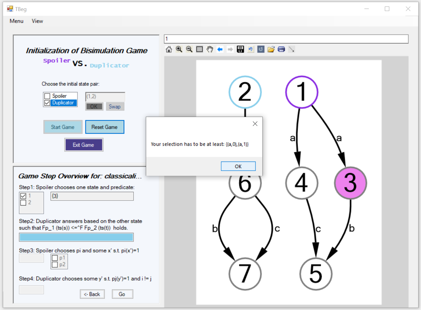
Figure 8: Screenshot of the graphical user interface with a game being played.

Next, the computer takes over the remaining role and the game starts: In the game overview, the user is guided through the steps by using two colors to indicate whether it is spoiler’s (violet) or duplicator’s (cyan) turn (see Figure 8).

In the case of two non-bisimular states, the tool will display a distinguishing formula at the end of the game.

5.2 Design

We now give an overview over the design and the relevant methods within the tool. We will also explain what has to be done in order to integrate a new functor.

T-Beg is a Windows tool offering a complete graphical interface, developed in Microsoft’s Visual Studio using $C\#$, especially Generics. It uses a graph library, which in turn provides a GraphEditor that allows for storing graphs as MSAGL files or as png and jpg files.

The program is divided into five components: Model, View, Controller, Game and Functor. We have chosen MVC (Model View Controller) as a modular pattern, so modules can be exchanged. Here we have several $\mathit{Model\langle T\rangle}$ managed by the $\mathit{Controller}$, where the functor in the sense of a Functor class, which always implements the Functor Interface, is indicated by the parameter $\langle T\rangle$.

While the tool supports more general functors, there is specific support for functors $F$ with $F=V^{G(-)}$ where $V$ specifies a semiring and $G$ preserves finite sets. That is, $F$ describes the branching type of a weighted transition system, where for instance $G=A\times(-)+1$ (introducing finitely many labels and termination). Coalgebras are of the form $X\to V^{GX}$ or – via currying – of the form $X\times GX\to V$, which means that they can be represented by $X\times GX$-matrices (matrices with index sets $X$, $GX$). In the implementation $V$ is the generic data type of the matrix entries. In the case of the powerset functor we simply have $V=2$ and $G=\mathit{Id}$.

If the branching type of the system can not simply be modelled as a matrix, there is an optional field that can be used to specify the system, since $\mathit{Model\langle T\rangle}$ calls the user-implemented method to initialize the $F$-coalgebra instance. The implementation of Algorithm 1 can be found in $\mathit{Game}\langle T,V\rangle$, representing the core of the tool’s architecture, whose correctness is only guaranteed for functors that meet our requirements, such as the functors used in the paper.

5.2.1 Functor Interface

As mentioned previously, the user has to provide nine methods in order to implement the functor in the context of T-Beg: two are needed for the computation, two for rendering the coalgebra as a graph, one for creating modal formulas, another two for loading and saving, and two more for customizing the visual matrix representation.

We would like to emphasize here that the user is free to formally implement the functor in the sense of the categorical definition as long as the nine methods needed for the game are provided. In particular, we do not need the application of the functor to arrows since we only need to lift predicates $p:X\rightarrow 2$.

Within $\mathit{MyFunctor}$, which implements the interface $\mathit{Functor\langle F,V\rangle}$, the user defines the data structure $F$ for the branching type of the transition system (e.g., a list or bit vector for the powerset functor, or the corresponding function type in the case of the distribution functor). Further, the user specifies the type $V$ that is needed to define the entries of $X\times GX$ (e.g. a double value for a weight or $0,1$ to indicate the existence of a transition).

Then the following nine methods has to be provided:

$\mathit{Matrix\langle F,V\rangle InitMatrix(\dots)}$:

This method initializes the transition system with the string-based input of the user. The information about the states and the alphabet is provided via an input mask in the form of a matrix.

$\mathit{bool\ CheckDuplicatorsConditionStep2(\dots)}$: given two states $x_{0},x_{1}$ and two predicates $p_{0},p_{1}$, this method checks whether

$$Fp_{0}(\alpha(x_{0}))\leq^{F}Fp_{1}(\alpha(x_{1})).$$

This method is used when playing the game (in Step $2$) and in the partition refinement algorithm (Algorithm 1) for the case $p_{0}=p_{1}$.

$\mathit{TSToGraph(\dots)}$: This method handles the implementation of the graph-based visualization of the transition system. For weighted systems the user can rely on the default implementation included within the Model. In this case, arrows between states and their labels are generated automatically.

$\mathit{GraphToTS(\dots)}$: This method is used for the other direction, i.e. to derive the transition system from a directed graph given by $\mathit{Graph}$.

$\mathit{string\ GetModalityToString(\dots)}$: This method is essential for the automatic generation of the modal logical formulas distinguishing two non-bisimilar states as described in Definition 5. In each call, the cone modality that results from $F\chi_{P}(\alpha(s))$ with $T(x_{0},x_{1})=(s,P)$ is converted into a string.

$\mathit{SaveTransitionSystem(\dots)}$: In order to store a transition system in a csv file.

$\mathit{LoadTransitionSystem(\dots)}$: In order to load a transition system from a csv file.

$\mathit{GetRowHeadings(\dots)}$: T-Beg can visualize a transition system $\alpha:X\rightarrow FX$ as a $X\times GX$ matrix within a DataGrid. For this purpose, the user needs to specify how the RowHeaders can be generated automatically.

$\mathit{ReturnRowCount(\dots)}$: This method returns the number of rows of the matrix representing the coalgebra.

The implementation costs arising on the user side can be improved by employing a separate module that automatically generates functors (see [7]). But it is not clear whether the lifting of the preorder can be obtained automatically. Nevertheless, a combination of [7] and [18] featuring T-Beg would result in a very powerful coalgebraic tool framework.

6 Conclusion and Discussion

Our aim in this paper is to give concrete recipes for explaining non-bisimilarity in a coalgebraic setting. This involves the computation of the winning strategy of the spoiler in the bisimulation game, based on a partition refinement algorithm, as well as the generation of distinguishing formulas, following the ideas of [6]. Furthermore we have presented a tool that implements this functionality in a generic way. Related tools, as mentioned in [10], are limited to labelled transition systems and mainly focus on the spoiler strategy instead of generating distinguishing formulas.

In the future we would like to combine our prototype implementation with an efficient coalgebraic partition refinement algorithm, adapting the ideas of Kanellakis/Smolka [15] or Paige/Tarjan [22] or using the existing coalgebraic generalization [9], thus enabling the efficient computation of winning strategies and distinguishing formulae.

For the generation of distinguishing formulas, an option would be to fix the modalities a priori and to use them in the game, similar to the notion of $\lambda$-bisimulation [11, 19]. However, there might be infinitely many modalities and the partition refinement algorithm can not iterate over all of them. A possible solution would be to find a way to check the conditions symbolically in order to obtain suitable modalities.

Of course we are also interested in whether we can lift the extra assumptions that were necessary in order to re-code modalities in Section 4.3. We also expect that the bisimulation game can be extended to polyadic predicate liftings.

An interesting further idea is to translate the coalgebra into multi-neighbourhood frames [13, 20], based on the predicate liftings, and to derive a $\lambda$-bisimulation game as in [19, 11] from there. (The $\lambda$-bisimulation game does not require weak pullback preservation and extends the class of admissible functors, but requires us to fix the modalities rather than generate them.) One could go on and translate these multi-neighbourhood frames into Kripke frames, but this step unfortunately does not preserve bisimilarity.

We also plan to study applications where we can exploit the fact that the distinguishing formula witnesses non-bisimilarity. For instance, we see interesting uses in the area of differential privacy [5], for which we would need to generalize the theory to a quantitative setting. That is, we would like to construct distinguishing formulas in the setting of quantitative coalgebraic logics, which characterize behavioural distances.

Acknowledgements

We would like to thank the reviewers for the careful reading of the paper and their valuable comments. Furthermore we thank Thorsten Wißmann and Sebastian Küpper for inspiring discussions on (efficient) coalgebraic partition refinement and zippability.

Appendix 0.A Proofs

References

- [1] Balan, A., Kurz, A.: Finitary functors: From Set to Preord and Poset. In: Proc. of CALCO ’11. pp. 85–99. Springer (2011), LNCS 6859
- [2] Baltag, A.: Truth-as-Simulation: Towards a Coalgebraic Perspective on Logic and Games. Tech. Rep. SEN-R9923, CWI (November 1999)
- [3] Baltag, A.: A logic for coalgebraic simulation. In: Coalgebraic Methods in Computer Science, CMCS 2000. ENTCS, vol. 33, pp. 42–60. Elsevier (2000)
- [4] Barr, M.: Relational algebras. In: Proc. Midwest Category Seminar. LNM, vol. 137. Springer (1970)
- [5] Chatzikokolakis, K., Gebler, D., Palamidessi, C., Xu, L.: Generalized Bisimulation Metrics. In: Proc. of CONCUR ’14. Springer (2014), LNCS/ARCoSS 8704
- [6] Cleaveland, R.: On Automatically Explaining Bisimulation Inequivalence. In: Proc. of CAV ’90. pp. 364–372. Springer (1990), LNCS 531
- [7] Deifel, H.P., Milius, S., Schröder, L., Wißmann, T.: Generic Partition Refinement and Weighted Tree Automata. In: ter Beek, M.H., McIver, A., Oliveira, J.N. (eds.) Formal Methods – The Next 30 Years. pp. 280–297. Springer International Publishing, Cham (10 2019)
- [8] Desharnais, J., Laviolette, F., Tracol, M.: Approximate analysis of probabilistic processes: Logic, simulation and games. In: Proc. of QEST ’08. pp. 264–273. IEEE (2008)
- [9] Dorsch, U., Milius, S., Schröder, L., Wißmann, T.: Efficient Coalgebraic Partition Refinement. In: Proc. of CONCUR 2017. LIPIcs, Schloss Dagstuhl - Leibniz-Zentrum fuer Informatik (2017)
- [10] de Frutos Escrig, D., Keiren, J.J.A., Willemse, T.A.C.: Games for Bisimulations and Abstraction (2016), https://arxiv.org/abs/1611.00401, arXiv:1611.00401
- [11] Gorín, D., Schröder, L.: Simulations and Bisimulations for Coalgebraic Modal Logics. In: Proc. of CALCO ’13. pp. 253–266. Springer (2013), LNCS 8089
- [12] Hansen, H., Kupke, C.: A coalgebraic perspective on monotone modal logic. In: Coalgebraic Methods in Computer Science, CMCS 2004. LNCS, vol. 106, pp. 121–143. Elsevier (2004)
- [13] Hansen, H.H.: Monotonic Modal Logics. Master’s thesis, University of Amsterdam (2003)
- [14] Hennessy, M., Milner, A.: Algebraic Laws for Nondeterminism and Concurrency. Journal of the ACM 32(1), 137–161 (Jan 1985)
- [15] Kanellakis, P.C., Smolka, S.A.: CCS Expressions, Finite State Processes, and Three Problems of Equivalence. Information and Computation 86, 43–68 (1990)
- [16] Komorida, Y., Katsumata, S.Y., Hu, N., Klin, B., Hasuo, I.: Codensity Games for Bisimilarity. In: Proc. of LICS ’19. pp. 1–13. ACM (2019)
- [17] König, B., Küpper, S.: A Generalized Partition Refinement Algorithm, Instantiated to Language Equivalence Checking for Weighted Automata. Soft Computing 22(4) (2018)
- [18] König, B., Küpper, S., Mika, C.: PAWS: A Tool for the Analysis of Weighted Systems. In: Proceedings 15th Workshop on Quantitative Aspects of Programming Languages and Systems, QAPL@ETAPS 2017, Uppsala, Sweden, 23rd April 2017. pp. 75–91 (2017)
- [19] König, B., Mika-Michalski, C.: (Metric) Bisimulation Games and Real-Valued Modal Logics for Coalgebras. In: Proc. of CONCUR ’18. LIPIcs, vol. 118, pp. 37:1–37:17. Schloss Dagstuhl – Leibniz Center for Informatics (2018)
- [20] Kracht, M., Wolter, F.: Normal Monomodal Logics Can Simulate All Others. The Journal of Symbolic Logic 64(1), 99–138 (1999)
- [21] Kupke, C.: Terminal Sequence Induction via Games. In: Prof. of TbiLLC ’07 (International Tbilisi Symposium on Language, Logic and Computation). pp. 257–271. Springer (2009), LNAI 5422
- [22] Paige, R., Tarjan, R.E.: Three Partition Refinement Algorithms. SIAM Journal on Computing 16(6), 973–989 (1987)
- [23] Pattinson, D.: Coalgebraic modal logic: soundness, completeness and decidability of local consequence. Theoretical Computer Science 309(1), 177 – 193 (2003)
- [24] Pattinson, D.: Expressive logics for coalgebras via terminal sequence induction. Notre Dame Journal of Formal Logic 45, 19–33 (2004)
- [25] Rutten, J.: Universal coalgebra: a theory of systems. Theoretical Computer Science 249(1), 3 – 80 (2000)
- [26] Schröder, L.: Expressivity of coalgebraic modal logic: The limits and beyond. Theoretical Computer Science 390(2), 230 – 247 (2008)
- [27] Stirling, C.: Bisimulation, modal logic and model checking games. Logic Journal of the IGPL 7(1), 103–124 (01 1999)
- [28] Trnková, V.: General theory of relational automata. Fundamenta Informaticae 3, 189–234 (1980)
- [29] Wißmann, T.: Personal communication
- [30] Wißmann, T.: Coalgebraic Semantics and Minimization in Sets and Beyond. Ph.D. thesis, Friedrich-Alexander-Universität Erlangen-Nürnberg (2020)