$\beta$ decay of even-A nuclei within the interacting boson model based on nuclear density functional theory

Abstract

We compute the $\beta$-decay $ft$-values within the frameworks of the energy density functional (EDF) and the interacting boson model (IBM). Based on the constrained mean-field calculation with the Gogny-D1M EDF, the IBM Hamiltonian for an even-even nucleus and essential ingredients of the interacting boson-fermion-fermion model (IBFFM) for describing the neighboring odd-odd nucleus are determined in a microscopic way. Only the boson-fermion and residual neutron-proton interaction strengths are determined empirically. The Gamow-Teller (GT) and Fermi (F) transition rates needed to compute the $\beta$-decay $ft$-values are obtained without any additional parameter or quenching of the $g_{A}$ factor. The observed $\log{ft}$ values for the $\beta^{+}$ decays of the even-even Ba into odd-odd Cs nuclei, and of the odd-odd Cs to the even-even Xe nuclei, with mass $A\approx 130$ are reasonably well described. The predicted GT and F transition rates represent a sensitive test of the quality of the IBM and IBFFM wave functions.

I Introduction

The $\beta$ decay of atomic nuclei is a consequence of electro-weak fundamental processes and its ability to convert protons in neutrons and vice-versa make it a very relevant reaction mechanism in many nuclear physics scenarios. For instance, it plays an important role in modeling the creation of elements in astrophysical nucleosynthesis scenarios. Precise measurement and the theoretical description of the (single) $\beta$ decay are also crucial to better estimating the matrix element of the $\beta\beta$ decay, especially the one that does not emit neutrinos (neutrino-less $\beta\beta$ decay), a rare event that would signal the existence of physics beyond the Standard Model of elementary particles Faessler and Simkovic (1998); Engel and Menéndez (2017).

The quantitative understanding of the $\beta$ decay process requires a good and consistent description of the low-lying spectrum of both parent and daughter nuclei. A variety of theoretical methods have been used for this purpose. Without trying to be exhaustive, we can mention the quasiparticle random phase approximation (QRPA) used at various levels of sophistication Sarriguren et al. (2001); Šimkovic et al. (2013); Pirinen and Suhonen (2015); Marketin et al. (2016); Mustonen and Engel (2016); Nabi and Böyükata (2016), the beyond mean-field approaches within the nuclear energy density functional (EDF) framework Rodríguez and Martínez-Pinedo (2010); Yao et al. (2015), the description based on large-scale interacting shell model calculations Langanke and Martínez-Pinedo (2003); Caurier et al. (2005); Honma et al. (2005); Shimizu et al. (2018); Yoshida et al. (2018), or that based on the interacting boson model (IBM) Dellagiacoma and Iachello (1989); Navrátil and Dobe (1988); Iachello and Van Isacker (1991); Yoshida et al. (2002); Zuffi et al. (2003); Brant et al. (2004, 2006); Barea and Iachello (2009); Yoshida and Iachello (2013); Mardones et al. (2016). Each of the theoretical methods have their own advantages and drawbacks that defined their range of applicability in the nuclear chart.

In the present work, we employ the IBM framework with input from microscopic EDF calculations Nomura et al. (2008). Our principal aim is a consistent theoretical description of the low-lying states and $\beta$ decay of even-A nuclei, including even-even and odd-odd ones. Within this approach, the potential energy surface (PES) for a given even-even nucleus is computed microscopically by means of the constrained mean-field method based on a nuclear EDF. The mean-field PES is mapped onto the expectation value of the IBM Hamiltonian in the intrinsic state of the $s$ (with spin and parity $0^{+}$) and $d$ ($2^{+}$) boson system. This procedure completely determines the strength parameters of the IBM Hamiltonian, which provides excitation spectra and transition strengths in arbitrary nuclear systems. The method can be extended to odd-mass and odd-odd nuclear systems by using the particle-boson coupling scheme. In such an extension, an additional EDF mean-field calculation is carried out to provide the required spherical single-particle energies and occupation numbers for unpaired nucleon(s) in the odd-A or odd-odd nucleus. Those mean-field quantities represent an essential input to build the Hamiltonian of the interacting boson-fermion-fermion model (IBFFM) Brant et al. (1984); Iachello and Van Isacker (1991). The strength parameters for the boson-fermion and residual neutron-proton coupling terms are determined so as to reproduce reasonably well the experimental low-energy spectra in the neighboring odd-A nucleus, and the odd-odd nucleus of interest. At the price of having to determine these few coupling constants empirically, the method allows for a systematic, detailed and simultaneous description of spectroscopy in even-even, odd-A, and odd-odd nuclei in a computationally feasible manner as also required in $\beta$ decay studies.

In Ref. Nomura et al. (2020a), we implemented the EDF-based interacting boson-fermion model (IBFM) Iachello and Scholten (1979); Iachello and Van Isacker (1991) approach in the study of the $\beta$ decay of odd-A nuclei. There we studied the allowed $\beta$ decays, where the spin of the parent nucleus changes according to the $\Delta I=0,\pm 1$ rule and parity is conserved. Both the Gamow-Teller (GT) and Fermi (F) transition strengths were considered in the evaluation of the $ft$ values of the $\beta$ decay. One of the advantages of our approach is that the calculation for the GT and F transition rates does not involve any additional free parameter, and that can be considered a very stringent test for the IBFM wave functions for the parent and daughter nuclei.

In the present work, since we are focusing in $\beta$ decay between even-mass nuclei, the calculation of the $ft$-values requires the IBM and IBFFM wave functions for the parent and daughter (or vise versa) even-even and odd-odd nuclei, respectively. Calculation of the single-$\beta$ decay between such even-A nuclei is also required for computing the $\beta\beta$ decay nuclear matrix elements, which are suggested to occur between a number of even-even nuclei. As in Ref. Nomura et al. (2020a), we consider the $\beta$ decays of those nuclei in the $A\approx 130$ mass region. There are a number of (phenomenological) IBFM calculations for the low-lying states and $\beta$ decay of odd-A nuclei. However, application of the IBFFM framework to the spectroscopy in odd-odd nuclear systems has rarely been pursued, let alone their $\beta$ decays. To the best of our knowledge, the IBFFM has been employed to study the $\beta$ decays only in Refs. Brant et al. (2006) and Yoshida and Iachello (2013). The former study is a first attempt to implement IBFFM in the $\beta$ decay of even-even system, but only one nucleus ¹²⁴Ba was considered there. In the latter reference, two-neutrino $\beta\beta$ decays from Te to Xe isotopes was explored. The results of both studies are encouraging, since they show that the IBFFM framework is capable of describing the $\beta$ decay of even-A nuclei, even though the IBFFM Hamiltonian was determined in a fully phenomenological way.

We have used the parametrization D1M Goriely et al. (2009) of the Gogny-EDF J. Decharge and M. Girod and D. Gogny (1975); Robledo et al. (2019) for the microscopic calculation of the PES. Previous studies, using the EDF-to-IBM mapping procedure, have shown that the Gogny-D1M EDF provides a reasonable description of the spectroscopic properties of odd-A and odd-odd nuclei Nomura et al. (2017a, b, 2019, 2020b) in variety of mass regions including medium mass and heavy nuclei.

This paper is outlined as follows. In Sec. II we briefly describe the procedures to build the IBFFM Hamiltonians from the constrained Gogny-EDF calculations, and introduce the $\beta$ decay operators. The results of our calculations for the low-lying energy levels of the even-even Xe and Ba, and odd-odd Cs nuclei are briefly reviewed in Sec. III. The $\log{ft}$ values obtained for the $\beta$ decays of the studied even-A nuclei are discussed in Sec. IV. Finally, Sec. V is devoted to the summary and the concluding remarks.

II Theoretical framework

II.1 Hamiltonian

Let us first introduce the IBFFM Hamiltonian $\hat{H}$ for odd-odd systems. Note that we use the version of the IBFFM (called IBFFM-2) that distinguishes between neutron and proton degrees of freedom. The IBFFM-2 Hamiltonian consists of the IBM (called IBM-2) Hamiltonian $\hat{H}_{\text{B}}$ for an even-even nucleus, the Hamiltonians $\hat{H}_{\text{F}}^{\rho}$ for the odd neutron ($\rho=\nu$) and proton ($\rho=\pi$), the Hamiltonians $\hat{H}^{\rho}_{\text{BF}}$ that couple the odd neutron and the odd proton to the IBM-2 core, and finally the residual neutron-proton interaction $\hat{V}_{\text{res}}$:

$$\hat{H}_{\text{}}=\hat{H}_{\text{B}}+\hat{H}_{\text{F}}^{\nu}+\hat{H}_{\text{F}}^{\pi}+\hat{H}_{\text{BF}}^{\nu}+H_{\text{BF}}^{\pi}+\hat{V}_{\text{res}}.$$ (1)

The IBM-2 Hamiltonian reads:

$$\hat{H}_{\text{B}}=\epsilon(\hat{n}_{d_{\nu}}+\hat{n}_{d_{\pi}})+\kappa\hat{Q}_{\nu}\cdot\hat{Q}_{\pi}$$ (2)

where $\hat{n}_{d_{\rho}}=d^{\dagger}_{\rho}\cdot\tilde{d}_{\rho}$ is the $d$-boson number operator, and $\hat{Q}_{\rho}=d_{\rho}^{\dagger}s_{\rho}+s_{\rho}^{\dagger}\tilde{d}_{\rho}^{\dagger}+\chi_{\rho}(d^{\dagger}_{\rho}\times\tilde{d}_{\rho})^{(2)}$ is the quadrupole operator. The parameters of the Hamiltonian are denoted by $\epsilon$, $\kappa$, $\chi_{\nu}$, and $\chi_{\pi}$. The doubly-magic nucleus ¹³²Sn is taken as the inert core for the boson space. The numbers of neutron $N_{\nu}$ and proton $N_{\pi}$ bosons are computed as the numbers of neutron-hole and proton-particle pairs, respectively Otsuka et al. (1978). In the following, we will simplify the notation and we will refer to the IBM-2 and IBFFM-2 Hamiltonians simply as IBM and IBFFM, respectively.

The single-nucleon Hamiltonian $\hat{H}_{\text{F}}^{\rho}$ is given as

$$\hat{H}_{\text{F}}^{\rho}=-\sum_{j_{\rho}}\epsilon_{j_{\rho}}\sqrt{2j_{\rho}+1}(a_{j_{\rho}}^{\dagger}\times\tilde{a}_{j_{\rho}})^{(0)}$$ (3)

with $\epsilon_{j_{\rho}}$ being the single-particle energy of the odd nucleon. Here, $j_{\nu}$ ($j_{\pi}$) stands for the angular momentum of the single neutron (proton). The fermion creation and annihilation operators are denoted by $a_{j_{\rho}}^{(\dagger)}$ and $\tilde{a}_{j_{\rho}}$, with $\tilde{a}_{jm}=(-1)^{j-m}a_{j-m}$. For the fermion valence space, we consider the full neutron and proton major shell $N,Z=50-82$, i.e., the $3s_{1/2}$, $2d_{3/2}$, $2d_{5/2}$, $1g_{7/2}$, and $1h_{11/2}$ orbitals.

The boson-fermion coupling Hamiltonian $\hat{H}_{\text{BF}}^{\rho}$ takes the form:

$$\hat{H}_{\text{BF}}^{\rho}=\Gamma_{\rho}\hat{Q}_{\rho^{\prime}}\cdot\hat{q}_{\rho}+\Lambda_{\rho}\hat{V}_{\rho^{\prime}\rho}+A_{\rho}\hat{n}_{d_{\rho}}\hat{n}_{\rho}$$ (4)

where $\rho^{\prime}\neq\rho$. The first, second, and third terms in the expression above are the quadrupole dynamical, exchange, and monopole terms, respectively. The strength parameters are denoted by $\Gamma_{\rho}$, $\Lambda_{\rho}$, and $A_{\rho}$. As in previous studies Scholten (1985); Arias et al. (1986) we assume that both the quadrupole dynamical and exchange terms are dominated by the interaction between unlike particles (i.e., between the odd neutron and proton bosons and between the odd proton and neutron bosons). On the other hand, for the monopole term we only consider the interaction between like-particles (i.e., between the odd neutron and neutron bosons and between the odd proton and proton bosons). The bosonic quadrupole operator $\hat{Q}_{\rho}$ in Eq. (4) has been defined in Eq. (2). The fermionic quadrupole operator $\hat{q}_{\rho}$ reads:

$$\hat{q}_{\rho}=\sum_{j_{\rho}j^{\prime}_{\rho}}\gamma_{j_{\rho}j^{\prime}_{\rho}}(a^{\dagger}_{j_{\rho}}\times\tilde{a}_{j^{\prime}_{\rho}})^{(2)},$$ (5)

where $\gamma_{j_{\rho}j^{\prime}_{\rho}}=(u_{j_{\rho}}u_{j^{\prime}_{\rho}}-v_{j_{\rho}}v_{j^{\prime}_{\rho}})Q_{j_{\rho}j^{\prime}_{\rho}}$ and $Q_{j_{\rho}j^{\prime}_{\rho}}=\langle l\frac{1}{2}j_{\rho}||Y^{(2)}||l^{\prime}\frac{1}{2}j^{\prime}_{\rho}\rangle$ represents the matrix element of the fermionic quadrupole operator in the considered single-particle basis. The exchange term $\hat{V}_{\rho^{\prime}\rho}$ in Eq. (4) reads:

$$\hat{V}_{\rho^{\prime}\rho}= -(s_{\rho^{\prime}}^{\dagger}\tilde{d}_{\rho^{\prime}})^{(2)}\cdot\Bigg{\{}\sum_{j_{\rho}j^{\prime}_{\rho}j^{\prime\prime}_{\rho}}\sqrt{\frac{10}{N_{\rho}(2j_{\rho}+1)}}\beta_{j_{\rho}j^{\prime}_{\rho}}\beta_{j^{\prime\prime}_{\rho}j_{\rho}}$$

$$:((d_{\rho}^{\dagger}\times\tilde{a}_{j^{\prime\prime}_{\rho}})^{(j_{\rho})}\times(a_{j^{\prime}_{\rho}}^{\dagger}\times\tilde{s}_{\rho})^{(j^{\prime}_{\rho})})^{(2)}:\Bigg{\}}+(H.c.),$$

with $\beta_{j_{\rho}j^{\prime}_{\rho}}=(u_{j_{\rho}}v_{j^{\prime}_{\rho}}+v_{j_{\rho}}u_{j^{\prime}_{\rho}})Q_{j_{\rho}j^{\prime}_{\rho}}$. In the second line of the expression above the notation $:(\cdots):$ indicates normal ordering. The definition of the number operator for the odd fermion in the monopole interaction has already appeared in Eq. (3).

For the residual neutron-proton interaction $\hat{V}_{\text{res}}$, we adopted the following form

$$\hat{V}_{\text{res}}=4\pi u_{\rm D}\delta({\bf r})+u_{\rm T}\Bigg{\{}\frac{3(\sigma_{\nu}\cdot{\bf r})(\sigma_{\pi}\cdot{\bf r})}{r^{2}}-\sigma_{\nu}\cdot\sigma_{\pi}\Bigg{\}},$$ (7)

where the first and second terms denote the delta and tensor interactions, respectively. We have found that these two terms are enough to provide a reasonable description of the low-lying states in the considered odd-odd nuclei. Note that by definition ${\bf r}={\bf r_{\nu}}-{\bf r_{\pi}}$ and that $u_{\rm D}$ and $u_{\rm T}$ are the parameters of this term. Furthermore, the matrix element $V_{\text{res}}^{\prime}$ of the residual interaction $\hat{V}_{\text{res}}$ can be expressed as Yoshida and Iachello (2013):

$$V_{\text{res}}^{\prime} =(u_{j_{\nu}^{\prime}}u_{j_{\pi}^{\prime}}u_{j_{\nu}}u_{j_{\nu}}+v_{j_{\nu}^{\prime}}v_{j_{\pi}^{\prime}}v_{j_{\nu}}v_{j_{\nu}})V^{J}_{j_{\nu}^{\prime}j_{\pi}^{\prime}j_{\nu}j_{\pi}}$$

$${}-(u_{j_{\nu}^{\prime}}v_{j_{\pi}^{\prime}}u_{j_{\nu}}v_{j_{\pi}}+v_{j_{\nu}^{\prime}}u_{j_{\pi}^{\prime}}v_{j_{\nu}}u_{j_{\pi}})$$

$$\times\sum_{J^{\prime}}(2J^{\prime}+1)\left\{\begin{array}[]{ccc}{j_{\nu}^{\prime}}&{j_{\pi}}&J^{\prime}\\ {j_{\nu}}&{j_{\pi}^{\prime}}&J\end{array}\right\}V^{J^{\prime}}_{j_{\nu}^{\prime}j_{\pi}j_{\nu}j_{\pi}^{\prime}},$$ (10)

where

$$V^{J}_{j_{\nu}^{\prime}j_{\pi}^{\prime}j_{\nu}j_{\pi}}=\langle j_{\nu}^{\prime}j_{\pi}^{\prime};J|\hat{V}_{\text{res}}|j_{\nu}j_{\pi};J\rangle$$ (11)

represents the matrix element between the neutron-proton pair with angular momentum $J$. The bracket in Eq. (II.1) represents the corresponding Racah coefficient. As was done in Ref. Morrison et al. (1981), the terms resulting from contractions are neglected in Eq. (II.1).

The matrix form of the IBFFM Hamiltonian of Eq. (1) is obtained in the basis $\ket{[L_{\nu}\otimes L_{\pi}]^{(L)}\otimes[j_{\nu}\otimes j_{\pi}]^{(J)}]^{(I)}}$. Here, $L_{\rho}$ is the angular momentum of proton or neutron boson system, $L$ is the total angular momentum of the boson system, and $I$ is the total angular momentum of the coupled boson-fermion-fermion system.

II.2 Procedure to build the IBFFM Hamiltonian

As the first step to build the IBFFM Hamiltonian, we have carried out (constrained) Hartree-Fock-Bogoliubov (HFB) calculations, based on the parametrization D1M of the Gogny-EDF. Those HFB calculations provide the potential energy surfaces (PESs), in terms of the quadrupole deformation parameters $\beta$ and $\gamma$, for the even-even core nuclei ^124-132Xe and ^124-132Ba. For a given nucleus, the Gogny-D1M PES is then mapped onto the expectation value of the IBM-2 Hamiltonian in the boson coherent state Ginocchio and Kirson (1980) (see, Refs. Nomura et al. (2008, 2010), for details). This mapping procedure uniquely determines the parameters $\epsilon$, $\kappa$, $\chi_{\nu}$, and $\chi_{\pi}$ in the boson Hamiltonian. Their values have already been given in Ref. Nomura et al. (2020a).

Second, the single-particle energies $\epsilon_{j_{\nu}}$ ($\epsilon_{j_{\pi}}$) and occupation probabilities $v^{2}_{j_{\nu}}$ ($v^{2}_{j_{\pi}}$) of the unpaired neutron (proton) for the neighboring odd-N (odd-Z) nucleus are computed with the help of Gogny-D1M HFB calculations constrained to zero deformation Nomura et al. (2017a). Those energies are used as input to the Hamiltonians $\hat{H}_{\mathrm{F}}^{\nu}$ ($\hat{H}_{\mathrm{F}}^{\pi}$) and $\hat{H}_{\mathrm{BF}}^{\nu}$ ($\hat{H}_{\mathrm{BF}}^{\pi}$), for the odd-$N$ Xe and odd-$Z$ Cs isotopes, respectively. The optimal values of the strength parameters for the boson-fermion Hamiltonian $\hat{H}_{\mathrm{BF}}^{\nu}$ ($\hat{H}_{\mathrm{BF}}^{\pi}$), i.e., $\Gamma_{\nu}$, $\Lambda_{\nu}$, and $A_{\nu}$ ($\Gamma_{\pi}$, $\Lambda_{\pi}$, and $A_{\pi}$), are chosen separately for positive and negative parity, so as to reproduce the experimental low-energy spectrum for each of the considered odd-$N$ Xe (odd-$Z$ Cs) nuclei.

Third, the use the previous strength parameters $\Gamma_{\nu}$, $\Lambda_{\nu}$, and $A_{\nu}$ ($\Gamma_{\pi}$, $\Lambda_{\pi}$, and $A_{\pi}$) for the IBFFM Hamiltonian for the odd-odd nuclei ^124-132 Cs. In this case, the values of $\epsilon_{j_{\rho}}$ and $v^{2}_{j_{\rho}}$ are calculated again for each of these odd-odd nuclei. The employed boson-fermion interaction strengths, and $\epsilon_{j_{\rho}}$ and $v^{2}_{j_{\rho}}$ for the odd-odd Cs nuclei can be found in Ref. Nomura et al. (2020b). Finally, the strength parameters for the residual neutron-proton interaction, $u_{\text{D}}=0.7$ MeV and $u_{\text{T}}=0.02$ MeV, are taken also from Ref. Nomura et al. (2020b).

II.3 Gamow-Teller and Fermi transition operators

To obtain the $\beta$-decay $ft$-values, the Gamow-Teller (GT) and Fermi (F) matrix elements should be computed by using the IBM and IBFFM wave functions that correspond to the initial state (with spin $\ket{I_{\mathrm{i}}}$) for the parent nucleus and the final state (with spin $\ket{I_{\mathrm{f}}}$) for the daughter nucleus, or vice versa. The building blocks are the following one-fermion transfer operators Dellagiacoma and Iachello (1989):

$$A^{(j)\dagger}_{m} =\zeta_{j}a_{jm}^{\dagger}+\sum_{j^{\prime}}\zeta_{jj^{\prime}}s^{\dagger}_{\rho}(\tilde{d}_{\rho}\times a_{j^{\prime}}^{\dagger})^{(j)}_{m}$$ (12)

$$B^{(j)\dagger}_{m} =\theta_{j}s^{\dagger}_{\rho}\tilde{a}_{jm}+\sum_{j^{\prime}}\theta_{jj^{\prime}}(d^{\dagger}_{\rho}\times\tilde{a}_{j^{\prime}})^{(j)}_{m}$$ (13)

Both operators increase the number of valence neutrons (protons) $n_{j}+2N_{\rho}$ by one. Note, that the index of $j_{\rho}$ is omitted for the sake of simplicity. The conjugate operators read:

$$\tilde{A}^{(j)}_{m}=\zeta_{j}^{*}\tilde{a}_{jm}+\sum_{j^{\prime}}\zeta_{jj^{\prime}}^{*}s_{\rho}(d^{\dagger}_{\rho}\times\tilde{a}_{j^{\prime}})^{(j)}_{m}$$ (14)

$$\tilde{B}^{(j)}_{m}=-\theta_{j}^{*}s_{\rho}a_{jm}^{\dagger}-\sum_{j^{\prime}}\theta_{jj^{\prime}}^{*}(\tilde{d}_{\rho}\times a_{j^{\prime}}^{\dagger})^{(j)}_{m}$$ (15)

These operators decrease the number of valence neutrons (protons) $n_{j}+2N_{\rho}$ by one.

The coefficients $\zeta_{j}$, $\zeta_{jj^{\prime}}$, $\theta_{j}$, and $\theta_{jj^{\prime}}$ in Eqs. (12)-(15) are given Iachello and Van Isacker (1991) by

$$\zeta_{j} =u_{j}\frac{1}{K_{j}^{\prime}},$$ (16)

$$\zeta_{jj^{\prime}} =-v_{j}\beta_{j^{\prime}j}\sqrt{\frac{10}{N_{\rho}(2j+1)}}\frac{1}{KK_{j}^{\prime}},$$ (17)

$$\theta_{j} =\frac{v_{j}}{\sqrt{N_{\rho}}}\frac{1}{K_{j}^{\prime\prime}},$$ (18)

$$\theta_{jj^{\prime}} =u_{j}\beta_{j^{\prime}j}\sqrt{\frac{10}{2j+1}}\frac{1}{KK_{j}^{\prime\prime}}.$$ (19)

The parameters $K$, $K_{j}^{\prime}$, and $K_{j}^{\prime\prime}$ entering the previous expressions read Dellagiacoma (1988); Dellagiacoma and Iachello (1989); Iachello and Van Isacker (1991):

$$K=\left(\sum_{jj^{\prime}}\beta_{jj^{\prime}}^{2}\right)^{1/2},$$ (20a)

$$K_{j}^{\prime}=\left(1+2\left(\frac{v_{j}}{u_{j}}\right)^{2}\frac{\braket{(\hat{n}_{s_{\rho}}+1)\hat{n}_{d_{\rho}}}_{0^{+}_{1}}}{N_{\rho}(2j+1)}\frac{\sum_{j^{\prime}}\beta_{j^{\prime}j}^{2}}{K^{2}}\right)^{1/2},$$ (20b)

$$K_{j}^{\prime\prime}=\left(\frac{\braket{\hat{n}_{s_{\rho}}}_{0^{+}_{1}}}{N_{\rho}}+2\left(\frac{u_{j}}{v_{j}}\right)^{2}\frac{\braket{\hat{n}_{d_{\rho}}}_{0^{+}_{1}}}{2j+1}\frac{\sum_{j^{\prime}}\beta_{j^{\prime}j}^{2}}{K^{2}}\right)^{1/2}$$ (20c)

In these definition, $\hat{n}_{s_{\rho}}$ is the number operator for the $s_{\rho}$ boson and $\braket{\cdots}_{0^{+}_{1}}$ represents the expectation value of a given operator in the $0^{+}_{1}$ ground state of the considered even-even nucleus. For a more detailed account, the reader is referred to Refs. Dellagiacoma (1988); Dellagiacoma and Iachello (1989); Iachello and Van Isacker (1991).

The boson images of the Fermi ($t^{\pm}$) and Gamow-Teller ($t^{\pm}\sigma$) transition operators, denoted by $\hat{O}^{\text{F}}$ and $\hat{O}^{\text{GT}}$, respectively, take the form

$$t^{\pm}\longmapsto\hat{O}^{\rm F}=-\sum_{j}\sqrt{2j+1}\left(P^{(j)}_{\nu}\times P^{(j)}_{\pi}\right)^{(0)},$$ (21)

$$t^{\pm}\sigma\longmapsto\hat{O}^{\rm GT}=\sum_{j^{\prime}j}\eta_{j^{\prime}j}\left(P^{(j^{\prime})}_{\nu}\times P^{(j)}_{\pi}\right)^{(1)}$$ (22)

where the $\eta_{j^{\prime}j}$ coefficients are proportional to the reduced matrix elements of the spin operator

$$\eta_{j^{\prime}j} =-\frac{1}{\sqrt{3}}\langle\ell^{\prime}\frac{1}{2};j^{\prime}||{\bf\sigma}||\ell\frac{1}{2};j\rangle$$

$$=-\delta_{\ell^{\prime}\ell}\sqrt{2(2j^{\prime}+1)(2j+1)}W\left(\ell j^{\prime}\frac{1}{2}1;\frac{1}{2}j\right),$$ (23)

with $W$ being a Racah coefficient. In the case of $\beta^{+}$ decay $P_{\nu}^{(j^{\prime})}=\tilde{B}_{\nu}^{(j^{\prime})}$ and $P_{\pi}^{(j)}=\tilde{A}_{\pi}^{(j)}$ while for $\beta^{-}$ decay $P_{\nu}^{(j^{\prime})}=B_{\nu}^{(j^{\prime})\dagger}$ and $P_{\pi}^{(j)}={A_{\pi}^{(j)\dagger}}$. Then, the reduced Fermi $\braket{M_{\text{F}}}$ and Gamow-Teller $\braket{M_{\text{GT}}}$ matrix elements read:

$$\braket{M_{\text{F}}}=\frac{1}{\sqrt{2I_{\mathrm{i}}+1}}|\langle I_{\mathrm{f}}||\hat{O}^{\mathrm{F}}||I_{\mathrm{i}}\rangle|$$ (24)

$$\braket{M_{\text{GT}}}=\frac{1}{\sqrt{2I_{\mathrm{i}}+1}}|\langle I_{\mathrm{f}}||\hat{O}^{\mathrm{GT}}||I_{\mathrm{i}}\rangle|$$ (25)

The $ft$-value for the $\beta$ decay $I_{\mathrm{i}}\rightarrow I_{\mathrm{f}}$, can be computed, in seconds, using the expression

$$ft=\frac{6163}{\braket{M_{\text{F}}}^{2}+g_{A}^{2}\braket{M_{\text{GT}}}^{2}}.$$ (26)

The quantity $g_{A}$ is the ratio of the axial-vector to vector coupling constants, $g_{A}=G_{A}/G_{V}$. We have employed the free nucleon value $g_{A}=1.2701(25)$ Beringer et al. (2012) for all the studied nuclei without quenching.

III Low-energy structure of the parent and daughter nuclei

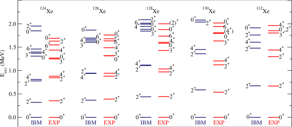
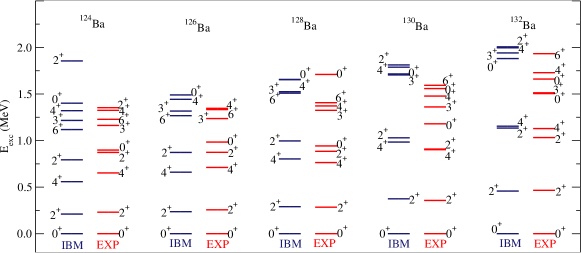
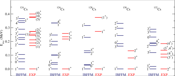
Figure 1: (Color online) Low-energy and low-spin excitation spectra for the even-even ^124-132Xe and ^124-132Ba, and the odd-odd ^124-132Cs nuclei considered in this work. The experimental data are taken from the compilation of the ENSDF database Brookhaven National Nuclear Data Center .

The low-lying level structure and electromagnetic properties of the even-even Ba and Xe, as well as odd-odd Cs, nuclei have already been discussed in detail in Ref. Nomura et al. (2020b). Also in this reference, the IBFM description of the neighboring odd-$N$ Ba and Xe as well as odd-$Z$ Cs isotopes has been amply discussed and shown to be also in reasonable agreement with experiment. The even-even ^124-132Xe nuclei are taken as the cores for the odd-odd ^124-132Cs nuclei. The Gogny-HFB PESs and mapped IBM description of these even-even Xe nuclei have shown that quite many of them are $\gamma$-soft Nomura et al. (2017b). Therefore, the low-energy spectra of the odd-odd Cs nuclei are described in terms of an unpaired neutron hole and a proton coupled to the $\gamma$-soft even-even core Xe nuclei. The low-energy positive-parity states of the odd-odd Cs nuclei, with excitation energies typically up to $E_{\text{exc}}\approx 0.4$ MeV, have been shown Nomura et al. (2020b) to be built on the $(\nu sdg)^{-1}\otimes(\pi sdg)^{1}$ neutron-proton pair configuration.

The low-energy spectra for the even-even ^124-132Ba and ^124-132Xe isotopes are shown in Fig. 1. The IBM description of the low-lying excited states of the even-even systems looks very nice. An exception is perhaps the excitation energy of the $0^{+}_{2}$ level in many of the Ba nuclei, which is overestimated by the calculation. This is because the Gogny-HFB PESs have a minimum at a rather large deformation leading to a rather pronounced rotational energy spectrum in the IBM calculation. Also in Fig. 1, the calculated and experimental positive-parity excitation spectra for the odd-odd ^124-132Cs nuclei are depicted up to 0.4 MeV excitation energy. Note that the energy spectra for the odd-odd Cs, shown in the figure, are taken from Ref. Nomura et al. (2020b) without any modification. Except for the ¹³²Cs nucleus, the IBFFM reproduces the correct ground-state spin. The calculation is not able to describe all the details of the lowest-lying level structures in each nucleus. But this is not surprising, considering the presence of both the unpaired neutron and proton degrees of freedom.

There are also those higher-spin positive-parity states with an excitation energy of $E_{\text{exc}}\geqslant 0.4$ MeV and with a spin typically $I\geqslant 6^{+}$. These high-spin states are mostly accounted for by the $(\nu h_{11/2})^{-1}\otimes(\pi h_{11/2})^{1}$ configuration, and are considered to be members of a chiral band. Note, however, that most of the $\beta$ decays considered in this work are relevant only for the low-spin states, i.e., $I\leqslant 4^{+}$, of the odd-odd Cs. Furthermore, the admixture of the $(\nu h_{11/2})^{-1}\otimes(\pi h_{11/2})^{1}$ pair configuration into the lowest-lying states is so small, that its effect on the $\beta$ decay rates from and to the ground states of the odd-odd Cs can be considered as negligible.

Other spectroscopic properties of the low-lying states of the even-even Xe and Ba and odd-odd Cs isotopes, such as the electric quadrupole and magnetic dipole moments and transition strengths, were described reasonably well Nomura et al. (2020b).

IV $\beta$ decay

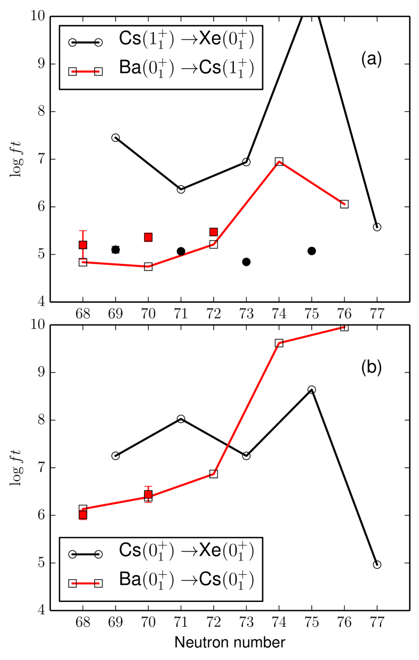
Figure 2: (Color online) The predicted $\log{ft}$ values (open symbols connected by solid lines) for the $\beta^{+}$ decays/EC (electron capture) between even-A nuclei, i.e., (a) Ba$(0^{+}_{1})\rightarrow$Cs$(1^{+}_{1})$, and Cs$(1^{+}_{1})\rightarrow$Xe$(0^{+}_{1})$, and (b) Ba$(0^{+}_{1})\rightarrow$Cs$(0^{+}_{1})$, and Cs$(0^{+}_{1})\rightarrow$Xe$(0^{+}_{1})$, plotted against the neutron number. The experimental $\log{ft}$ values, taken from the ENSDF database Brookhaven National Nuclear Data Center , are represented by filled circles (Cs$\rightarrow$Xe decays) and squares (Ba$\rightarrow$Cs decays).

IV.1 $\beta$ decays of even-even Ba

Table 1: The predicted and experimental $\log{ft}$ values in seconds for the $\beta^{+}$ decays/EC of the even-even ^124,126,128Ba into odd-odd ^124,126,128Cs nuclei. The experimental data have been taken from Ref. Brookhaven National Nuclear Data Center .

Decay	$I_{\mathrm{i}}\rightarrow I_{\mathrm{f}}$	$\log{ft}$
		Theory	Experiment
124 Ba$\rightarrow^{124}$ Cs	$0^{+}_{1}\rightarrow 0^{+}_{1}$	6.134	6.01(10)
	$0^{+}_{1}\rightarrow 1^{+}_{1}$	4.837	5.2(3)
	$0^{+}_{1}\rightarrow 1^{+}_{2}$	5.902	5.07(7)
	$0^{+}_{1}\rightarrow 1^{+}_{3}$	5.289	5.72(9)
	$0^{+}_{1}\rightarrow 1^{+}_{4}$	6.300	6.01(10)
	$0^{+}_{1}\rightarrow 1^{+}_{5}$	4.600	6.04(9)
	$0^{+}_{1}\rightarrow 1^{+}_{6}$	4.948	6.23(10)
	$0^{+}_{1}\rightarrow 1^{+}_{7}$	5.176	6.83(16)
	$0^{+}_{1}\rightarrow 1^{+}_{8}$	5.437	4.54(7)
126 Ba$\rightarrow^{126}$ Cs	$0^{+}_{1}\rightarrow 0^{+}_{1}$	6.348	6.44(17)
	$0^{+}_{1}\rightarrow 1^{+}_{1}$	4.744	5.36(9)
	$0^{+}_{1}\rightarrow 1^{+}_{2}$	4.823	6.36(12)
	$0^{+}_{1}\rightarrow 1^{+}_{3}$	5.392	5.49(5)
	$0^{+}_{1}\rightarrow 1^{+}_{4}$	5.624	6.44(17)
	$0^{+}_{1}\rightarrow 1^{+}_{5}$	4.538	5.18(6)
	$0^{+}_{1}\rightarrow 1^{+}_{6}$	6.028	5.12(7)
	$0^{+}_{1}\rightarrow 1^{+}_{7}$	8.944	5.08(8)
	$0^{+}_{1}\rightarrow 1^{+}_{8}$	10.810	4.54(7)
128 Ba$\rightarrow^{128}$ Cs	$0^{+}_{1}\rightarrow 0^{+}_{1}$	6.868
	$0^{+}_{1}\rightarrow 1^{+}_{1}$	5.201	5.471(9)
	$0^{+}_{1}\rightarrow 1^{+}_{2}$	4.858	8.26(11)
	$0^{+}_{1}\rightarrow 1^{+}_{3}$	5.324	7.83(5)
	$0^{+}_{1}\rightarrow 1^{+}_{4}$	7.823	5.57(4)
	$0^{+}_{1}\rightarrow 1^{+}_{5}$	4.776	7.83(9)
	$0^{+}_{1}\rightarrow 1^{+}_{6}$	6.784	7.33(7)
	$0^{+}_{1}\rightarrow 1^{+}_{7}$	8.595	6.68(6)

We show in Fig. 2 the predicted $\log{ft}$ values for the $\beta^{+}$ decay (electron-capture (EC)) of the even-A nuclei, that is, ^124-132 Ba$(0^{+}_{1})\rightarrow^{124-132}$ Cs$(1^{+}_{1})$, and ^124-132 Cs$(1^{+}_{1})\rightarrow^{124-132}$ Xe$(0^{+}_{1})$ (panel (a)), and ^124-132 Ba$(0^{+}_{1})\rightarrow^{124-132}$ Cs$(0^{+}_{1})$, and ^124-130 Cs$(0^{+}_{1})\rightarrow^{124-130}$ Xe$(0^{+}_{1})$ (panel (b)). The experimental data are taken from the ENSDF database Brookhaven National Nuclear Data Center and are also depicted in the figure. The calculated $\log{ft}$ values for the ground-state-to-ground-state decays $0^{+}_{1}$(Ba)$\rightarrow 1^{+}_{1}$(Cs) are in a very good agreement with the experiment. The $\log{ft}$ values for the $1^{+}_{1}$(Cs)$\rightarrow 0^{+}_{1}$(Xe) decays are, however, considerably overestimated. The $0^{+}_{1}\leftrightarrows 1^{+}_{1}$ decays involve only the GT transitions, and the $\braket{M_{\text{GT}}}^{2}$ values for these decays appear to be too small in our calculation. We will discuss below the reason for this small matrix elements. As for the $0^{+}_{1}\rightarrow 0^{+}_{1}$ decays (see, Fig. 2(b)), where only the Fermi transition enters, the present calculation gives a very good description of the experimental $\log{ft}$ values for the decays of ^124,126Ba into ^124,126Cs nuclei. A characteristic systematic trend of the predicted $\log{ft}$ value is that for both the $\Delta I=\pm 1$ (Fig. 2(a)) and $\Delta I=0$ (Fig. 2(b)) decays it changes abruptly between $N=72$ and $N=76$ (for the Ba$\rightarrow$Cs decays) and between $N=73$ and $N=77$ (for the Cs$\rightarrow$Xe decays). Such an abrupt change in the $\log{ft}$ values could reflect the evolution of nuclear structure between axially-symmetric and $\gamma$-soft deformed states. Accordingly, the structures of those wave functions for the boson-core Xe nuclei, as well as the neighboring odd-A Xe and Cs nuclei, are supposed to be very different between before and after the shape transition.

In Table 1, we make a more detailed comparison between the predicted and experimental $\log{ft}$ values for the $\beta^{+}$ decays of the $0^{+}_{1}$ ground states of even-even ^124,126,128Ba into those higher-lying states in odd-odd ^124,126,128Cs nuclei. Experimentally, there are many degenerate levels in those nuclei, and their spin and/or parities are also not firmly established. This makes very difficult to establish a one-to-one correspondence between the calculated and experimental $\log{ft}$ values. Those situations involving experimental degenerate levels are mentioned in the footnotes of Table 1. The same rule applies to Tables 2, 3, and 4, in the following Sec. IV.2. Among other things, we emphasize that, as seen from Table 1, a very good agreement between the predicted and experimental $\log{ft}$ values is obtained for the $\beta^{+}$ decays to the $1^{+}_{1}$ ground states of the ^124,126,128Cs nuclei. This situation is already shown in Fig. 2(a). In addition, the observed $\log{ft}$ values for the $0^{+}_{1}\rightarrow 0^{+}_{1}$ decays of ^124,126 Ba, where the GT transition is forbidden and only the Fermi transition enters, are well reproduced by our calculation. As for the $\log{ft}$ values for the decays into higher-energy, non-yrast $0^{+}$ and $1^{+}$ states, especially those higher than the 4-th lowest-energy ones for each spin, the discrepancy between the calculation and experiment increases. We can understand this trend by taking into account that the IBFFM is built in a reduced valence space, and the strength parameters are determined so as to fit the low-lying energy levels of odd-odd nuclei. Therefore, the wave functions for these higher non-yrast states in the present IBFFM calculation are not supposed to be as reliable as the ones of the lowest-energy states.

IV.2 $\beta$ decays of odd-odd Cs

Table 2: Same as Table 1, but for the $\beta^{+}$/EC decays of the odd-odd ¹²⁴Cs to even-even ¹²⁴Xe nuclei.

Decay	$I_{\mathrm{i}}\rightarrow I_{\mathrm{f}}$	$\log{ft}$
		Theory	Experiment
124 Cs$\rightarrow^{124}$ Xe	$1^{+}_{1}\rightarrow 0^{+}_{1}$	7.452	5.10(7)
	$1^{+}_{1}\rightarrow 0^{+}_{2}$	6.659	5.54(7)
	$1^{+}_{1}\rightarrow 0^{+}_{3}$	6.621	6.21(7)
	$1^{+}_{1}\rightarrow 0^{+}_{4}$	7.560	5.72(7)
	$1^{+}_{1}\rightarrow 0^{+}_{5}$	7.496	5.69(7)
	$1^{+}_{1}\rightarrow 0^{+}_{6}$	10.268	6.6(4)
	$1^{+}_{1}\rightarrow 1^{+}_{1}$	5.810	6.6(4)
	$1^{+}_{1}\rightarrow 1^{+}_{2}$	6.022	5.69(7)
	$1^{+}_{1}\rightarrow 2^{+}_{1}$	6.061	5.10(7)
	$1^{+}_{1}\rightarrow 2^{+}_{2}$	8.949	5.89(7)
	$1^{+}_{1}\rightarrow 2^{+}_{3}$	8.628	5.73(7)
	$1^{+}_{1}\rightarrow 2^{+}_{4}$	7.017	6.15(7)
	$1^{+}_{1}\rightarrow 2^{+}_{5}$	7.245	6.01(7)
	$1^{+}_{1}\rightarrow 2^{+}_{6}$	6.636	6.43(7)
	$1^{+}_{1}\rightarrow 2^{+}_{7}$	6.757	5.40(7)
	$1^{+}_{1}\rightarrow 2^{+}_{8}$	6.710	5.69(7)
	$7^{+}_{1}\rightarrow 6^{+}_{1}$	6.965	7.4
	$7^{+}_{1}\rightarrow 6^{+}_{2}$	7.797	7.7
	$7^{+}_{1}\rightarrow 6^{+}_{3}$	10.596	7.6
	$7^{+}_{1}\rightarrow 6^{+}_{4}$	8.341	6.2
	$7^{+}_{1}\rightarrow 6^{+}_{5}$	8.862	7.3
	$7^{+}_{1}\rightarrow 7^{+}_{1}$	7.761	7.6
	$7^{+}_{1}\rightarrow 7^{+}_{2}$	8.087	7.3
	$7^{+}_{1}\rightarrow 7^{+}_{3}$	8.693	6.7
	$7^{+}_{1}\rightarrow 7^{+}_{4}$	9.711	6.7
	$7^{+}_{1}\rightarrow 8^{+}_{1}$	7.654	7.3
	$7^{+}_{1}\rightarrow 8^{+}_{2}$	9.506	6.7
	$7^{+}_{1}\rightarrow 8^{+}_{3}$	8.634	6.7

Table 3: Same as Table 1, but for the $\beta^{+}$/EC decays of the odd-odd ¹²⁶Cs to even-even ¹²⁶Xe nuclei.

Decay	$I_{\mathrm{i}}\rightarrow I_{\mathrm{f}}$	$\log{ft}$
		Theory	Experiment
126 Cs$\rightarrow^{126}$ Xe	$1^{+}_{1}\rightarrow 0^{+}_{1}$	6.366	5.066(19)
	$1^{+}_{1}\rightarrow 0^{+}_{2}$	6.832	5.39(3)
	$1^{+}_{1}\rightarrow 0^{+}_{3}$	7.345
	$1^{+}_{1}\rightarrow 0^{+}_{4}$	7.084	6.93
	$1^{+}_{1}\rightarrow 0^{+}_{5}$	9.782	6.176(25)
	$1^{+}_{1}\rightarrow 0^{+}_{6}$	7.907	5.941(25)
	$1^{+}_{1}\rightarrow 0^{+}_{7}$	6.307	6.67(4)
	$1^{+}_{1}\rightarrow 0^{+}_{8}$	6.465
	$1^{+}_{1}\rightarrow 0^{+}_{9}$	9.447	6.09(3)
	$1^{+}_{1}\rightarrow 1^{+}_{1}$	6.161	$>$7.1
	$1^{+}_{1}\rightarrow 1^{+}_{2}$	7.639	6.93
	$1^{+}_{1}\rightarrow 1^{+}_{3}$	8.279	6.176(25)
	$1^{+}_{1}\rightarrow 2^{+}_{1}$	8.405	6.791(24)
	$1^{+}_{1}\rightarrow 2^{+}_{2}$	4.426	7.574(20)
	$1^{+}_{1}\rightarrow 2^{+}_{3}$	5.127	8.83(10)
	$1^{+}_{1}\rightarrow 2^{+}_{4}$	5.563	6.306(12)
	$1^{+}_{1}\rightarrow 2^{+}_{5}$	5.417	6.988(18)
	$1^{+}_{1}\rightarrow 2^{+}_{6}$	7.349	$>$7.1

Table 4: Same as Table 1, but for the $\beta^{+}$/EC decays of the odd-odd ^128,130,132Cs to even-even ^128,130,132Xe nuclei.

Decay	$I_{\mathrm{i}}\rightarrow I_{\mathrm{f}}$	$\log{ft}$
		Theory	Experiment
128 Cs$\rightarrow^{128}$ Xe	$1^{+}_{1}\rightarrow 0^{+}_{1}$	6.941	4.843(10)
	$1^{+}_{1}\rightarrow 0^{+}_{2}$	7.236	5.579(24)
	$1^{+}_{1}\rightarrow 0^{+}_{3}$	8.783	7.48(4)
	$1^{+}_{1}\rightarrow 0^{+}_{4}$	6.744	5.70(3)
	$1^{+}_{1}\rightarrow 1^{+}_{1}$	5.853	6.37(3)
	$1^{+}_{1}\rightarrow 1^{+}_{2}$	8.427	6.32(3)
	$1^{+}_{1}\rightarrow 1^{+}_{3}$	7.577	6.49(3)
	$1^{+}_{1}\rightarrow 2^{+}_{1}$	6.924	5.089(24)
	$1^{+}_{1}\rightarrow 2^{+}_{2}$	7.386	5.829(25)
	$1^{+}_{1}\rightarrow 2^{+}_{3}$	6.640	6.10(3)
	$1^{+}_{1}\rightarrow 2^{+}_{4}$	6.772	6.37(3)
	$1^{+}_{1}\rightarrow 2^{+}_{5}$	7.130	6.24(3)
	$1^{+}_{1}\rightarrow 2^{+}_{6}$	6.867	6.32(3)
	$1^{+}_{1}\rightarrow 2^{+}_{7}$	7.046	6.49(3)
130 Cs$\rightarrow^{130}$ Xe	$1^{+}_{1}\rightarrow 0^{+}_{1}$	10.523	5.073(6)
	$1^{+}_{1}\rightarrow 0^{+}_{2}$	6.334	7.0(1)
	$1^{+}_{1}\rightarrow 0^{+}_{3}$	6.711	6.2(1)
	$1^{+}_{1}\rightarrow 1^{+}_{1}$	6.800	6.9(2)
	$1^{+}_{1}\rightarrow 1^{+}_{2}$	8.373
	$1^{+}_{1}\rightarrow 2^{+}_{1}$	7.309	6.3(1)
	$1^{+}_{1}\rightarrow 2^{+}_{2}$	5.233	7.5(4)
	$1^{+}_{1}\rightarrow 2^{+}_{3}$	4.826	6.2(1)
	$1^{+}_{1}\rightarrow 2^{+}_{4}$	7.564	6.9(2)
132 Cs$\rightarrow^{132}$ Xe	$1^{+}_{1}\rightarrow 0^{+}_{1}$	5.575
	$1^{+}_{1}\rightarrow 0^{+}_{2}$	6.991
	$1^{+}_{1}\rightarrow 2^{+}_{1}$	6.375
	$1^{+}_{1}\rightarrow 2^{+}_{2}$	4.388
	$2^{+}_{1}\rightarrow 2^{+}_{1}$	6.364	6.679
	$2^{+}_{1}\rightarrow 2^{+}_{2}$	4.459	8.7(1)
	$2^{+}_{1}\rightarrow 2^{+}_{3}$	4.685	6.61(2)
	$2^{+}_{1}\rightarrow 3^{+}_{1}$	6.367	7.17(2)

Experimental data is more abundant for the $\beta^{+}$ decay of the odd-odd Cs isotopes. In Table 2, the predicted $\log{ft}$ values for the decays of the $1^{+}_{1}$ ground state of the ¹²⁴Cs nucleus into ¹²⁴Xe are compared with the experimental data. The $\log{ft}$ value for the decay to the $I_{f}=0^{+}_{1}$ ground state of ¹²⁴Xe is predicted to be unexpectedly larger than the experimental one. This means that the calculated GT transition rate is too small. The dominant pair configurations in the IBFFM wave function for the $1^{+}_{1}$ ground state are: $[(\nu s_{1/2})^{-1}\otimes(\pi s_{1/2})^{1}]^{(J=1^{+})}$ (14.2 %), $[(\nu s_{1/2})^{-1}\otimes(\pi d_{3/2})^{1}]^{(J=1^{+})}$ (10.8 %), $[(\nu s_{1/2})^{-1}\otimes(\pi d_{5/2})^{1}]^{(J=3^{+})}$ (12.8 %), and $[(\nu s_{1/2})^{-1}\otimes(\pi g_{7/2})^{1}]^{(J=3^{+})}$ (11.2 %). The rest of the wave function is made up of numerous other components that are so small in their magnitudes as to be neglected. The odd neutron occupying the $3s_{1/2}$ orbital makes dominant contributions to the above mentioned pair configurations. This seems to be consistent with the fact that the ${1/2}^{+}_{1}$ ground state of the neighboring odd-A nucleus ¹²³Xe is mostly accounted for by the $3s_{1/2}$ neutron hole coupled to the even-even core ¹²⁴Xe Nomura et al. (2020a).

Major contributions to the $\braket{M_{\text{GT}}}$ value for the $1^{+}_{1}\rightarrow 0^{+}_{1}$ decay of ¹²⁴Cs turn out to be from those terms proportional to $[a^{\dagger}_{j_{\nu}}\times a^{\dagger}_{j_{\pi}}]^{(1)}$, $[\tilde{d}_{\nu}\times[a^{\dagger}_{j_{\nu}}\times a^{\dagger}_{j_{\pi}}]]^{(1)}$, and $[\tilde{d}_{\nu}\times\tilde{d}_{\pi}]\times[a^{\dagger}_{j_{\nu}}\times a^{\dagger}_{j_{\pi}}]]^{(1)}$. Their matrix elements are calculated as $0.02886$, $-0.02576$, and $-0.02152$, respectively. Two of these matrix elements have almost the equal magnitude but with opposite sign, and this leads to the too small $\braket{M_{\text{GT}}}$ value. A similar kind of cancellation, among different components in $\braket{M_{\text{GT}}}$ seems to take place in the GT transitions to the non-yrast $0^{+}$ states of the daughter nucleus. In the previous IBFFM calculation for the $\beta$ decay of ¹²⁴Ba in Ref. Brant et al. (2006), the same kind of discrepancy (too large $\log{ft}$-values) was also found. The authors of Ref. Brant et al. (2006) also attributed it to the cancellations of small components in the GT matrix element. On the other hand, for the decays with $\Delta I=0$, i.e., $1^{+}_{1}\rightarrow 1^{+}_{1}$, the predicted $\log{ft}$ values are generally smaller and reproduce the experimental data better than for the $\Delta I=\pm 1$ decays. This is mainly because $\braket{M_{\text{F}}}$ matrix elements also appear in the denominator in the expression for the $ft$-value for the $1^{+}_{1}\rightarrow 1^{+}_{1}$ decays (see, Eq. (26).

In the case of the ¹²⁴Cs nucleus in particular, there are also the experimental data for the decays from the higher-spin state with $I_{\text{i}}=7^{+}$. In the present IBFFM calculation, those states with spin higher than $I\approx 7^{+}$ are formed mainly of the $(\nu h_{11/2})^{-1}\otimes(\pi h_{11/2})^{1}$ neutron-proton pair configuration. In contrast, the low-spin and low-energy states in the vicinity of the ground state and with $I\leqslant 4^{+}$ are mainly based on the neutron and proton positive-parity $sdg$ orbitals. The experimental $\log{ft}$ values for the decays of $7^{+}$ state are generally $\log{ft}\approx 7$, being larger than for the decays of the ground state $1^{+}_{1}$, which are typically $\log{ft}\approx 5\sim 6$. The description of the $\log{ft}$ values for this type of the $\beta$ decay in the present calculation appears to be good, at least for the decays to the few lowest levels in the daughter nucleus. We confirmed that, as expected, the configurations that involve the neutron and proton unique-parity $h_{11/2}$ single-particle orbitals make significant contributions to the $\braket{M_{\text{GT}}}$ matrix elements for the decays of the $I_{\text{i}}=7^{+}$ state.

The calculated $\log{ft}$ for the rest of the odd-odd Cs nuclei are shown in Table 3 and Table 4 and compared to the experimental data. Similarly to the ¹²⁴Cs $\rightarrow^{124}$Xe decay, the calculated $\log{ft}$ values for the decays of ^126-132 Cs, especially for the $\Delta I=\pm 1$ decays, are too large as compared with the experimental values. This appears to happen mainly because the cancellation between components of the $\braket{M_{\text{GT}}}$ matrix elements occurs to the extent that too small GT rates are obtained. On the other hand, the agreement with experimental data is relatively good for the $\Delta I=0$ decays. Note, that a extremely large deviation is found in the decay ¹³⁰ Cs$(1^{+}_{1})\rightarrow^{130}$ Xe$(0^{+}_{1})$ (see, Table 4 and also Fig. 2). The predicted $ft$-value for this decay is larger than the experimental one implying a difference in the half-life of 5 orders of magnitude. Regarding the decay of the ¹³²Cs nucleus, where experimentally the $2^{+}_{1}$ state is suggested to be the ground state, the present calculation reproduces very nicely the $\log{ft}$ value for the $2^{+}_{1}\rightarrow 2^{+}_{1}$ decay.

V Summary and concluding remarks

To summarize, the $\beta$ decays of even-$A$ nuclei are investigated within the EDF-based IBM approach. The even-even boson-core Hamiltonian, and essential building blocks of the particle-boson coupling Hamiltonians, i.e., single-particle energies and occupation probabilities of odd particles, are determined based on a fully-microscopic mean field calculation with the Gogny EDF. A few coupling constants for the boson-fermion Hamiltonians, and for the residual neutron-proton interaction, remain as the only free parameters of the model. They are determined as to reasonably reproduce the low-energy levels of each of the neighbouring odd-$A$ and odd-odd nuclei. The IBM and IBFFM wave functions obtained after diagonalization of the corresponding Hamiltonians for the parent and daughter nuclei are used to calculate Gamow-Teller and Fermi matrix elements, which are required to compute the $\beta$-decay $ft$-values. No additional parameter is introduced for the computations of the $ft$-values. The $g_{A}$ factor for the GT transition is not quenched in the present calculation.

The present work, as well as the preceding ones of Refs. Nomura et al. (2020b, a), show that the employed theoretical method provides an excellent descriptions of the low-lying levels and electromagnetic transition rates in the relevant even-even Ba and Xe and odd-odd Cs, we as well as the neighboring odd-A Ba, Xe, and Cs nuclei. The observed $\beta^{+}$ decays/electron captures of the ground state $0^{+}_{1}$ of the even-even ^124,126,128Ba into the $1^{+}_{1}$ ground states and $0^{+}_{1}$ states of ^124,126,128Cs are described very nicely. On the other hand, the $\log{ft}$ values for the $1^{+}\rightarrow 0^{+}$ decays of the odd-odd Cs into even-even Xe nuclei are, in general, predicted to be too large with respect to the experimental values. It is shown that the deviation occurs mainly because numerous small components in the GT matrix element $\braket{M_{\text{GT}}}$ cancel each other, leading to the too small GT transition rates. This is attributed to the combination of various factors in the adopted theoretical procedure, such as, the chosen boson-fermion coupling constants, residual neutron-proton interaction, and underlying microscopic inputs from the Gogny EDF.

The EDF-based IBM framework, employed here and in Ref. Nomura et al. (2020a), represents a computationally feasible theoretical method for studying simultaneously the low-energy excitations and fundamental processes in atomic nuclei. Especially, we consider the results for a single $\beta$ decay between even-mass nuclei quite encouraging, as they represent a crucial step toward the computation of the $\beta\beta$ decay nuclear matrix elements between even-even nuclei. Work along this direction is in progress and will be reported in near future.