Influence of hadronic resonances on the chemical freeze-out in heavy-ion collisions

Abstract

Detailed knowledge of the hadronic spectrum is still an open question, which has phenomenological consequences on the study of heavy-ion collisions. A previous lattice QCD study concluded that additional strange resonances are missing in the currently tabulated lists provided by the Particle Data Group (PDG). That study identified the list labeled PDG2016+ as the ideal spectrum to be used as an input in thermal-model-based analyses. In this work, we determine the effect of additional resonances on the freeze-out parameters of systems created in heavy-ion collisions. These parameters are obtained from thermal fits of particle yields and net-particle fluctuations. For a complete picture, we compare several hadron lists including both experimentally discovered and theoretically predicted states. We find that the inclusion of additional resonances mildly influences the extracted parameters – with a general trend of progressively lowering the temperature – but is not sufficient to close the gap in temperature between light and strange hadrons previously observed in the literature.

I Introduction

Determining the number of hadronic resonances and their corresponding properties has been a fundamental question in nuclear physics for decades. Experimentally, new resonances (and their decay channels) are measured through spectroscopy and an up-to-date compilation of those searches can be found in the Particle Data Group booklet Tanabashi et al. (2018). Each new particle is assigned a star on a scale of * to **** which indicates the experimental confidence of the measurement, where * states are the most uncertain and **** states are the most established. Theoretical calculations, such as Quark Models Capstick and Isgur (1986); Ebert et al. (2009), predict many more resonances beyond those experimentally measured. Furthermore, there have been general theoretical arguments, originally made by Hagedorn, that near a limiting temperature (now understood as the phase transition of the hadron gas into the Quark Gluon Plasma Cabibbo and Parisi (1975)) an exponentially increasing mass spectrum Hagedorn (1965) is expected, i.e. heavier and heavier resonances can form that decay almost immediately into their daughter particles. Using these so-called “Hagedorn states” and comparing thermodynamic quantities to lattice Quantum Chromodynamics (QCD) calculations, initial evidence was found that the older versions of the PDG were insufficient to describe the lattice results Noronha-Hostler et al. (2010a); Majumder and Muller (2010); Noronha-Hostler et al. (2012). With the particle production results published by the ALICE Collaboration (${\rm Pb-Pb}\,\,2.76\,{\rm TeV}$ Abelev et al. (2014); Adam et al. (2017) and preliminary ${\rm Pb-Pb}\,\,5.02\,{\rm TeV}$ Bellini (2019)) a new issue arose, the so-called “proton anomaly” wherein thermal model fits generally over-predict the proton yields while simultaneously under-predicting the yields of strange baryons. Fluctuation analyses show the same trend Bellwied et al. (2019); Bluhm and Nahrgang (2019); Bellwied et al. (2020). A number of possible solutions were suggested such as a flavor hierarchy of freeze-out temperatures between light and strange hadrons Bellwied et al. (2013), further missing Hagedorn states Bazavov et al. (2014); Noronha-Hostler and Greiner (2014a, b), final state reactions Rapp and Shuryak (2001); Steinheimer et al. (2013), in-medium effects Aarts et al. (2019) or corrections to the ideal HRG model Lo et al. (2018); Andronic et al. (2019).

In order to settle much of these debates on the number of hadron resonances, lattice calculations have played a vital role in recent years. Initial results from Ref. Bazavov et al. (2014) found evidence of missing strange resonances from first principle calculations. In a more recent work, using partial contributions to the QCD pressure of particles grouped according to their quantum numbers, the exact nature of the missing resonances was determined Alba et al. (2017). Evidence for the need of additional states was seen in certain sectors and even with their inclusion, the contribution of strange mesons still underestimates lattice QCD results. However, in Ref. Alba et al. (2017) it was shown that the Quark Model predicts too many states – in particular in the $\left|S\right|=2$ sector – and thus overestimates most of the partial pressures. The list which correctly reproduces the largest number of observables is the PDG2016+ list (see definition below). For completeness, in this manuscript we will also consider Quark Model states, in order to investigate the effect of including the largest possible number of resonances in the analyses.

It is worth mentioning that missing hadronic resonances have been found to affect a number of areas in heavy-ion collisions such as the transport coefficients $\eta/s$ and $\zeta/s$ Noronha-Hostler et al. (2009, 2012); Rais et al. (2019), and may somewhat affect collective flow Noronha-Hostler et al. (2014); Alba et al. (2018) and mildly improve the $\chi^{2}$ of thermal fits Noronha-Hostler et al. (2010b). In Ref. Alba et al. (2018) we incorporated these missing states from the PDG into a hydrodynamic model and found that they are able to improve the fits to particle spectra and $\langle p_{T}\rangle$. Similar results were found in Ref. Devetak et al. (2019).

In this follow-up paper, we compare different hadronic lists with an increasing number of states, performing fits of particle yield and fluctuation data from RHIC and the LHC. One of the most pressing questions is whether these new states can close the gap between light and strange freeze-out temperatures, as suggested in Ref. Bazavov et al. (2014). Initial explorations in this direction can be found in Refs. Chatterjee et al. (2013, 2017), where smaller particle resonance lists were used. We study a scenario with a freeze-out temperature common to all species, as well as one where different freeze-out temperatures result for strange and light species. In the case of fits to yields and their ratios we compare the fit quality from both scenarios.

This manuscript is organized as follows. In Section II we describe the different hadronic lists we utilize in this work. Moreover, we provide the details on how the decay properties of the resonant states were estimated, when not known experimentally. In Section III we briefly describe the HRG model and the data sets employed in the fits we perform. In Sections IV and V we show our results for fits to yields and ratios in the single and double freeze-out scenarios, respectively. In Section VI we study the chemical freeze-out from an analysis of net-particle fluctuations from the Beam Energy Scan (BES) at RHIC. We first analyze fluctuations of net-proton and net-charge, then those of net-kaon. Finally, in Section VII we present our conclusions.

The particle lists PDG2005, PDG2016, PDG2016+ and QM utilized in this work, together with the corresponding decay channels can be downloaded from the link provided in Ref. pdg .

II Different hadron lists

We consider the following lists of hadronic resonances. PDG2005: PDG from 2005 Eidelman et al. (2004); PDG2016: PDG **-**** states from 2016 Patrignani et al. (2016); PDG2016+: PDG *-**** states from 2016 Patrignani et al. (2016); and QM: PDG2016+ combined with additional Quark Model states from Refs. Capstick and Isgur (1986); Ebert et al. (2009). The comparison between PDG2005 and PDG2016 is performed to demonstrate the difference between earlier thermal fit models and modern day ones. The PDG2016+ is tested in thermal fits in this paper for the first time. One primary reason why this has not yet been done in the past is that many of the * and ** states do not have adequate decay channel and branching ratio information in order to describe all the particle interactions based only on experimental data. In this paper, we use phenomenology to fill in these gaps. For completeness, we consider a mixture of the PDG2016+ with the addition of Quark Model states that in Ref. Alba et al. (2017) appeared to fit some lattice QCD data well. Note that the list we label as QM does not exclusively contain states predicted by the Quark Model. We replaced the Quark Model states that are already known experimentally with the corresponding ones from the PDG2016+ list. In order to discern whether a state predicted by the Quark Model was already listed in the PDG, we considered states sharing the same quantum numbers (baryon number, strangeness, electric charge, isospin and spin degeneracy), with comparable masses (mass difference below $\sim 150\,\,{\rm MeV}$, or within $15\%$ of the mass of the PDG state, whichever is smaller). The issue with the decays is even more pronounced for the QM, where no decay channels are given. In this case we relied entirely on phenomenological approaches that are described in detail below.

II.1 Decay lists

In the PDG database Patrignani et al. (2016), only the relatively few established states are provided with an exhaustive set of decays, whereas most states are only given branching ratios which do not sum up to $100\%$. In this case, additional decays are listed as “dominant”, “seen” or “not seen”.

When considering the effect of resonance decays, we include all the strong decays listed by the PDG with a branching ratio of at least $\simeq 1\%$, but we do not include weak decays. When the listed branching ratios do not sum up to $100\%$, we assign the remaining percentage to an electromagnetic decay of the kind $N_{2}\rightarrow N_{1}+\gamma$ – where $N_{2}$ and $N_{1}$ are hadrons with the same quantum numbers, $N_{1}$ being the next state in descending mass order with compatible parity for such a decay. We decay resonances that lack quantitative information predominantly radiatively (as explained above), in order to populate the next state with known branching ratios.

The situation is different for the hadronic resonant states predicted by relativistic quark models, since these are not supplied with any information on their decay properties. In order to take into account the effect of these additional states on observables, we need to estimate their branching ratios.

Along the lines of the work done for the PDG states, we infer the branching ratios of the additional QM states using the following procedure. Every state is assigned a predominant radiative decay, analogously to PDG states with incomplete information. The remaining percentage is reserved for hadronic decays, for which we use linear extrapolation from known branching ratios of PDG particles with the same quantum numbers $B,~{}S,~{}I$ and $Q$ (baryon number, strangeness, isospin and electric charge).

The linear extrapolation is performed as follows. States from the PDG2016+ list are divided into “families” with the same quantum numbers, and all strong decay modes present in the family are grouped together. For each channel appearing in the family, a linear interpolation of its branching ratio as a function of the particle mass is performed. Then, QM states of the same family are assigned branching ratios by sampling the linear mass dependence constructed as explained above. At this point, all negative BR values are discarded, as well as all decays that violate mass conservation. Finally, the sum of branching ratios for strong decays is normalized and put together with the electromagnetic ones.

We emphasize here that for the QM states we have the least amount of information and, therefore, the largest amount of uncertainties.

III Thermal Fits and the Hadron Resonance Gas model

The study of chemical freeze-out we present here makes use of the Hadron Resonance Gas (HRG) model, which describes the hadronic phase below the transition temperature $T_{c}$ as a system of non-interacting particles Hagedorn (1965); Dashen et al. (1969); Venugopalan and Prakash (1992). The HRG model has a wide-spread applicability in heavy-ion studies in reproducing thermal particle abundances and lately also in providing results on fluctuations of conserved charges $(B,~{}Q,~{}S)$ Alba et al. (2014, 2015); Bellwied et al. (2019); Bluhm and Nahrgang (2019); Poberezhnyuk et al. (2019). Recently, these observables have been compared to the measured moments of net-particle distributions, and provided freeze-out temperatures which are compatible with the ones obtained by comparing the experimental data to lattice QCD calculations Alba et al. (2014); Karsch and Redlich (2011); Garg et al. (2013); Fu (2013); Borsanyi et al. (2013, 2014).

Historically, the HRG model has been widely employed to compare data on particle production for energies ranging from the AGS to the LHC Becattini et al. (2006, 2013); Cleymans et al. (2006); Torrieri and Rafelski (2007); Andronic et al. (2011); Braun-Munzinger et al. (2004); Andronic et al. (2006); Bhattacharyya et al. (2019, 2020). Produced particle yields $\langle N_{i}\rangle$ are obtained by adding the contribution from resonances to the primordial thermal yield, given by $Vn_{i}$:

$$\langle N_{i}\rangle~{}=~{}V\,n_{i}~{}+~{}V\,\sum_{R}\langle n_{i}\rangle_{R}\,n_{R}~{}.$$ (1)

In the above, $\langle n_{i}\rangle_{R}$ is the average number of particles of type $i$ resulting from a decay of resonance $R$, $n_{i}$ and $n_{R}$ are thermal densities calculated through the statistical model, and $V$ is the system volume. Conditions on the net-strangeness and net-charge density are imposed, to match the heavy-ion collision situation:

$$\langle n_{S}(T;\mu_{B},\mu_{Q},\mu_{S})\rangle=0\,\,,$$

$$\langle n_{Q}(T;\mu_{B},\mu_{Q},\mu_{S})\rangle=\dfrac{Z}{A}\langle n_{B}\rangle\,\,.$$ (2)

These allow one to constrain the three chemical potentials. In this way, yields and ratios calculated within the HRG model only depend on the thermal parameters $(T,\mu_{B})$ (and $V$ in the case of yields).

Thermal properties at the chemical freeze-out have been studied using yields and ratios from STAR data in Au-Au collisions at $\sqrt{s_{\mathrm{NN}}}=200,~{}130,~{}39,~{}27,~{}19.6,~{}11.5,~{}7.7$ GeV Abelev et al. (2009); Adams et al. (2007); Adamczyk et al. (2017); Cleymans et al. (2005) and from ALICE data in Pb-Pb collisions at $\sqrt{s_{\mathrm{NN}}}=2.76\,{\rm TeV}$ and $5.02\,{\rm TeV}$ Abelev et al. (2013a, 2014, b, 2015); Andronic et al. (2018); Bellini (2019).

In this manuscript, we focus on the STAR data at $\sqrt{s_{\mathrm{NN}}}=200$ GeV and $0-5\%$ centrality, and the ALICE data at $\sqrt{s_{\mathrm{NN}}}=5.02$ TeV and $0-10\%$ centrality. We perform thermal fits of the particle yields and ratios, using published data on ratios, if available, for STAR Abelev et al. (2009) and for ALICE. In order to build the remaining ratios, published data on yields from both collaborations have been used with a proper propagation of the errors in the final result. We evaluate the yields and ratios for each hadronic list and extract the thermal parameters $(T,~{}\mu_{B},~{}V)$ by using the thermal fit package FIST Vovchenko and Stoecker (2019). The package allows users to choose their own particle lists, as well as data sets, in the fit.

IV Single Freeze-out Scenario

Initially, we consider a common freeze-out temperature for strange and light hadrons. We fit the measured yields for the following particles: $\pi^{+},~{}\pi^{-},~{}K^{+},~{}K^{-},~{}p,~{}\bar{p},~{}\Lambda,~{}\bar{\Lambda},~{}\phi,~{}\Xi,~{}\bar{\Xi},~{}\Omega,~{}\bar{\Omega}$ at the LHC, while at RHIC the separate $\Omega$ and $\bar{\Omega}$ yields are replaced by the sum $\Omega+\bar{\Omega}$. When we take the ratios, we divide the light particle yields by the yield of either $\pi^{+}$ or $\pi^{-}$ and the strange particle yields by the yield of either $K^{+}$ or $K^{-}$. The results of the thermal fits for both yields and ratios while varying the particle resonance list are shown in Table 1 for LHC data at $\sqrt{s_{NN}}=5.02\,{\rm TeV}$ and in Table 2 for STAR data at $\sqrt{s_{NN}}=200\,{\rm GeV}$. At the LHC we hold $\mu_{B}=1\,{\rm MeV}$ fixed to avoid the possibility of negative chemical potentials and remain consistent with previous analyses Andronic et al. (2013).

	T [MeV]		$\mu_{B}$ [MeV]		Volume [$\,{\rm fm}^{3}$]	$\chi^{2}$/DOF
	Yields	Ratios	Yields	Ratios	Yields	Yields	Ratios
PDG2005	158.3 $\pm$ 1.8	$155.7\pm 1.6$	1	1	4904 $\pm$ 456	74.0/11	80.7/12
PDG2016	152.1 $\pm$ 1.7	$149.2\pm 1.4$	1	1	5811 $\pm$ 545	102.4/11	111.5/12
PDG2016+	150.4 $\pm$ 1.5	$148.1\pm 1.3$	1	1	6250 $\pm$ 561	79.0/11	89.0/12
QM	147.9 $\pm$ 1.4	$146.0\pm 1.2$	1	1	6867 $\pm$ 581	64.7/11	75.0/12

Table 1: Temperatures and baryon chemical potential (fixed to 1 MeV) in the single chemical freeze-out scenario. The results are obtained from thermal fits to total yields and ratios from ALICE data (Bellini (2019)) at $0-10\%$ centrality in PbPb collisions, at $\sqrt{s_{NN}}=5.02\,{\rm TeV}$, using different particle lists. For the case of total yields, the volume is shown as well. The last two columns show the chi square per number of degrees of freedom in the fits.

	T [MeV]		$\mu_{B}$ [MeV]		Volume [$\,{\rm fm}^{3}$]	$\chi^{2}$/DOF
	Yields	Ratios	Yields	Ratios	Yields	Yields	Ratios
PDG2005	160.2 $\pm$ 2.1	$164.0\pm 2.7$	23.2 $\pm$ 8.1	$24.4\pm 9.3$	2251 $\pm$ 260	42.9/9	15.6/10
PDG2016	159.8 $\pm$ 2.3	$161.6\pm 2.8$	22.5 $\pm$ 7.2	$24.1\pm 8.6$	1984 $\pm$ 270	32.0/9	16.3/10
PDG2016+	156.4 $\pm$ 2.2	$158.5\pm 2.5$	21.1 $\pm$ 6.6	$23.1\pm 8.3$	2248 $\pm$ 304	14.5/9	8.7/10
QM	151.5 $\pm$ 1.8	$154.0\pm 2.1$	20.3 $\pm$ 6.6	$22.4\pm 8.2$	2768 $\pm$ 333	18.4/9	8.8/10

Table 2: Temperatures and baryon chemical potentials from thermal fits with a single chemical freeze-out scenario compared to either ratios or total yields from STAR data Abelev et al. (2009); Adams et al. (2007) for $0-5\%$ centrality in AuAu collisions at $\sqrt{s_{NN}}=200\,{\rm GeV}$, using different particle lists. For the case of total yields, the volume is shown as well. The last two columns show the chi square per number of degrees of freedom in the fits.

From Tables 1 and 2 a few trends begin to emerge:

• for both yields and ratios, more hadronic states generally decrease the chemical freeze-out temperature;

• the chemical freeze-out temperatures from yields and ratios approximately agree;

• generally, due to the decrease of the chemical freeze-out temperature with the increase of the number of hadronic states, the volume increases accordingly;

• $\mu_{B}$ is relatively stable when changing the particle resonance list;

• RHIC appears to have somewhat higher chemical freeze-out temperatures compared to the LHC;

• the inclusion of resonant states beyond the PDG2016+ list improves the fit quality at the LHC for both yields and ratios, while at RHIC the PDG2016+ fits best for the yields and the QM and PDG2016+ are equivalent for the ratios.

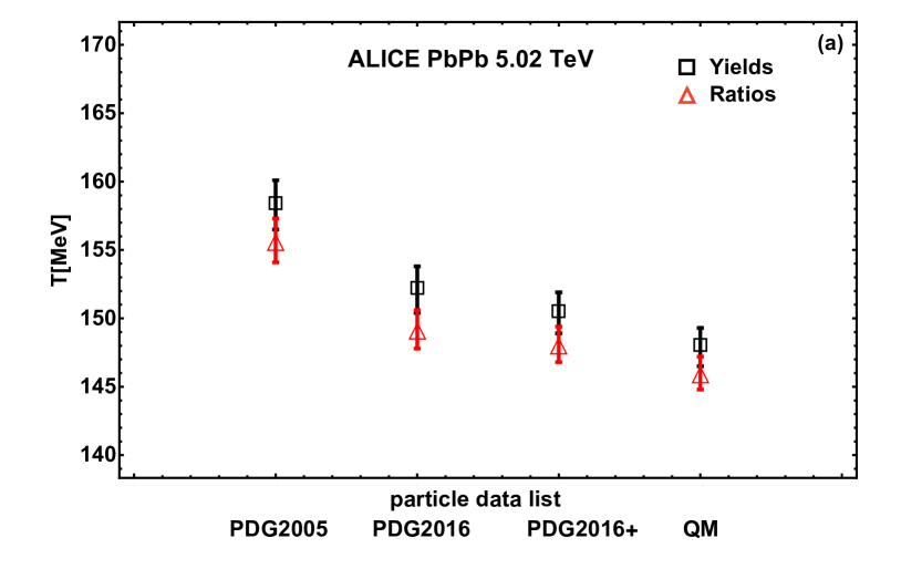
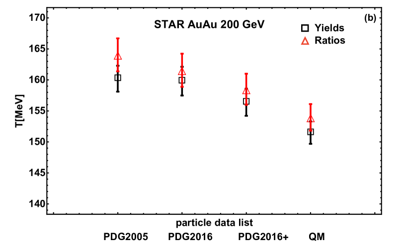
Figure 1: Dependence of the chemical freeze-out temperature on the particle data lists at the LHC (upper panel) and RHIC (lower panel). We compare the results extracted from yields (black squares) and ratios (red triangles).

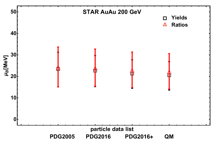
Figure 2: Dependence of $\mu_{B}$ on the particle data lists at RHIC. We compare the results extracted from yields (black squares) and the ratios (red triangles).

The second to last point is puzzling because one expects the freeze-out curves to remain roughly constant at low baryon chemical potential, according to lattice QCD studies of the phase transition at finite $\mu_{B}$ Bellwied et al. (2015); Bazavov et al. (2017).

The values of temperature and chemical potential listed in Tables 1 and 2 are shown in Fig. 1 and Fig. 2, respectively.

In Fig. 1, the decreasing trend of the chemical freeze-out temperature with the increasing number of hadronic states in the list is clearly visible. As mentioned previously, slightly higher temperatures are found at RHIC. On the other hand, in Fig. 2 we can see that the RHIC freeze-out chemical potential barely changes with different resonance lists, and that the results from yields and ratios agree well.

V Two Freeze-out Scenario

		T [MeV]		$\mu_{B}$ [MeV]		Volume [$\,{\rm fm}^{3}$]	$\chi^{2}$
		Yields	Ratios	Yields	Ratios	Yields	Yields	Ratios
PDG2005	Light	148.8 $\pm$ 2.2	144.9 $\pm$ 2.0	1	1	7598 $\pm$ 837	17.1/4	0.058/5
	Strange	167.5 $\pm$ 2.2	167.5 $\pm$ 2.0	1	1	3212 $\pm$ 335	23.8/7	20.1/8
PDG2016	Light	143.2 $\pm$ 1.8	140.3 $\pm$ 1.6	1	1	9096 $\pm$ 897	15.8/4	0.062/5
	Strange	169.8 $\pm$ 2.6	169.8 $\pm$ 2.3	1	1	2472 $\pm$ 319	7.2/7	6.1/8
PDG2016+	Light	142.5 $\pm$ 1.7	139.8 $\pm$ 1.6	1	1	9374 $\pm$ 902	14.7/4	0.063/5
	Strange	165.0 $\pm$ 2.4	164.7 $\pm$ 2.1	1	1	2978 $\pm$ 377	0.77/7	0.70/8
QM	Light	140.9 $\pm$ 1.6	138.5 $\pm$ 1.5	1	1	9961 $\pm$ 927	14.0/4	0.063/5
	Strange	158.5 $\pm$ 1.9	158.5 $\pm$ 1.7	1	1	3835 $\pm$ 433	0.12/7	0.10/8

Table 3: Temperatures and baryon chemical potential (fixed to 1 MeV) in the double chemical freeze-out scenario obtained from fits to ratios or total yields from ALICE data Bellini (2019) for $0-10\%$ centrality in PbPb collisions at $\sqrt{s_{NN}}=5.02$ TeV, using different PDG lists. For the case of total yields, the volume is shown as well. The last two columns show the chi square per number of degrees of freedom in the fits.

		T [MeV]		$\mu_{B}$ [MeV]		Volume [$\,{\rm fm}^{3}$]	$\chi^{2}$
		Yields	Ratios	Yields	Ratios	Yields	Yields	Ratios
PDG2005	Light	162.4 $\pm$ 7.0	$159.5\pm 6.2$	$23.9\pm 14.6$	$24.1\pm 10.7$	1943 $\pm$ 589	3.1/3	0.12/4
	Strange	160.0 $\pm$ 2.6	$165.0\pm 2.9$	$23.1\pm 9.8$	$24.3\pm 18.3$	2284 $\pm$ 362	42.8/5	14.8/6
PDG2016	Light	153.6 $\pm$ 5.1	$151.8\pm 4.7$	$22.6\pm 14.1$	$23.2\pm 10.3$	2528 $\pm$ 650	3.1/3	0.16/4
	Strange	161.0 $\pm$ 3.0	$166.1\pm 3.2$	$21.3\pm 8.9$	$22.4\pm 17.1$	1880 $\pm$ 352	28.4/5	10.1/6
PDG2016+	Light	152.5 $\pm$ 4.9	$150.9\pm 4.5$	$22.4\pm 13.9$	$23.0\pm 10.2$	2631 $\pm$ 654	2.9/3	0.18/4
	Strange	158.4 $\pm$ 3.1	$161.7\pm 2.9$	$20.3\pm 7.8$	$21.0\pm 14.7$	1981 $\pm$ 403	12.7/5	4.5/6
QM	Light	150.1 $\pm$ 4.5	$148.8\pm 4.1$	$22.0\pm 13.8$	$22.7\pm 10.1$	2860 $\pm$ 679	2.9/3	0.23/4
	Strange	152.4 $\pm$ 2.5	$155.8\pm 2.4$	$19.5\pm 7.8$	$20.3\pm 14.8$	2600 $\pm$ 474	17.8/5	6.5/6

Table 4: Temperatures and baryon chemical potentials in the double chemical freeze-out scenario obtained from fits to ratios or total yields from STAR data Abelev et al. (2009); Adams et al. (2007) for $0-5\%$ centrality in AuAu collisions at $\sqrt{s_{NN}}=200$ GeV, using different PDG lists. For the case of total yields, the volume is shown as well. The last two columns show the chi square per number of degrees of freedom in the fits.

We now explore the possibility of a flavor hierarchy between light and strange particles, using the same particle resonance lists as in the previous section. There, we saw that the Quark Model list produces the best fit to the experimental data at ALICE, while at RHIC the PDG2016+ provided the best fit for the yields and for the ratios the QM and PDG2016+ list were nearly equivalent. Nevertheless, we stress here again that the QM results are shown here just for illustration, as in Ref. Alba et al. (2017) it was found that the QM contains too many states and fails to reproduce several thermodynamic quantities from lattice QCD. For this analysis, we allow for two separate chemical freeze-out temperatures as well as two separate freeze-out baryon chemical potentials for light and strange particles.

For the light hadron fit we use $\pi^{+}$, $\pi^{-}$, $p$, $\overline{p}$, $K^{+}$ and $K^{-}$, while for the strange hadrons fit we use all species except pions and (anti)protons. We construct the ratios of strange hadrons dividing by the $K^{\pm}$ yields, to avoid mixing of light and strange degrees of freedom. We do this also because, if light particles freeze-out at a lower temperature than the one for strange particles, the respective volumes would be different and thus would not cancel out when taking ratios. In Tables 3 and 4 the extracted chemical freeze-out temperatures, chemical potentials and volumes (for yields only, as before) are shown for both the light and strange hadrons at the LHC and RHIC, respectively. As in the case of a single freeze-out scenario, there is very good agreement between fits to yields and ratios. Moreover, the freeze-out temperature for strange hadrons is systematically higher than that of light hadrons.

An additional effect of the two temperatures is that the light temperature is significantly lower than in the single freeze-out temperature scenario. This means that the fit in that case is driven by the strange states, as it was discussed in Alba et al. (2015). We also notice that the inclusion of more resonances affects the strange freeze-out temperature more than the light one. This is not unexpected, as most of the additional states carry strangeness.

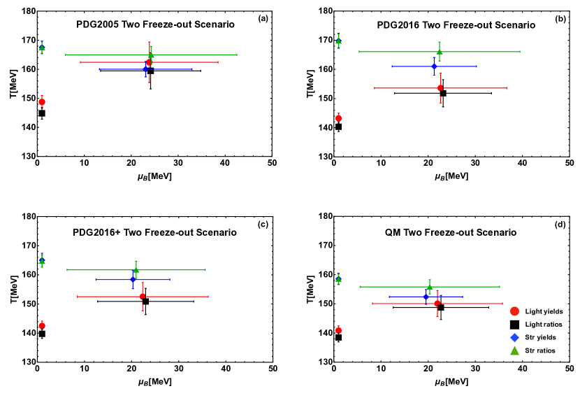
Figure 3: (Color online) Extracted light and strange freeze-out temperatures and chemical potentials from yields and ratios at the LHC and RHIC, in the case of a double freeze-out scenario. Each panel corresponds to a different particle list.

A summary of our results from Tables 3 and 4 is shown in Fig. 3, for yields and ratios from both ALICE and STAR, and with the four different hadron lists we consider. In this pictorial representation, the separation in temperature between strange and light freeze-out appears very clearly, especially from fits to LHC data. In this case, all lists lead to a very pronounced separation. In the case of STAR data, the separation is especially evident when utilizing the PDG2016 and PDG2016+ lists, although still present even for fits with the QM list. There seems to be a general trend in these last three hadron lists, where the presence of more states leads to a smaller separation of the strange and light freeze-out temperatures. The PDG2005 list is excluded from this trend: it contains a significantly smaller number of resonances, which is not realistic in modern calculations. On the other hand, we also know that the strange states contained in the QM list are too numerous, as noted earlier and shown in Ref. Alba et al. (2017).

In Appendix A (Figs. 5-8) a comparison of the yields and ratios to experimental data is shown, both in the single (red lines) and double (blue dotted lines) freeze-out scenarios.

VI Freeze-out from fluctuations

In this Section we complete our analysis by studying net-particle fluctuations from the BES at RHIC. We employ the state-of-the-art list PDG2016+ to perform the analysis of net-proton and net-charge fluctuations from Ref. Alba et al. (2014), as well as the analysis of net-kaon fluctuations from Ref. Bellwied et al. (2019). Both analyses were originally carried out with an older PDG list, which we here indicate as PDG2012.

In order to determine both the temperature and chemical potential at the chemical freeze-out, in general two experimental quantities are required. However, due to the large experimental errors on higher order fluctuations  (i.e., the ratio $\chi_{3}/\chi_{2}$) as noted in Adam et al. (2020); Koch (2010), in Ref. Bellwied et al. (2019) we obtained the freeze-out parameters as follows. Starting from the net-proton and net-charge freeze-out parameters obtained in Ref. Alba et al. (2014), we followed the isentropic trajectories determined in Ref. Gunther et al. (2017) via a Taylor-expanded equation of state from lattice QCD. These were constructed by first determining the entropy-per-baryon ratio at the freeze-out point for each collision energy from Ref. Alba et al. (2014), and then following the path that conserves $S/N_{B}$. The ratio $\chi^{K}_{1}/\chi^{K}_{2}$ was then calculated along these trajectories , and compared to the experimental results. For each collision energy, the overlap region will then correspond to the freeze-out points for net-kaons, which are shown in Fig. 4 in gray, while the red points correspond to the net-proton and net-charge freeze-out points from Ref. Alba et al. (2014).

In order to repeat the analysis with the PDG2016+ list, we first calculated the freeze-out parameters for light hadrons via a combined fit of $\chi_{1}^{p}/\chi_{2}^{p}$ and $\chi_{1}^{Q}/\chi_{2}^{Q}$ with the new list. We then used these light freeze-out parameters to determine the new isentropic trajectories in the QCD phase diagram. As was done in Ref. Gunther et al. (2017), we utilized a Taylor-expanded equation of state from lattice QCD. With the new isentropic trajectories, we could then calculate the net-kaon fluctuations along them and determine the freeze-out parameters.

We note that, both for the net-proton and net-charge, as well as for the net-kaon analysis, we included the effect of resonance decays, and imposed the same kinematic cuts employed in the experiments Adamczyk et al. (2014a, b, 2018). Moreover, for the light hadron analysis we included the effect of isospin randomization Kitazawa and Asakawa (2012a, b), which has a large impact on net-proton fluctuations.

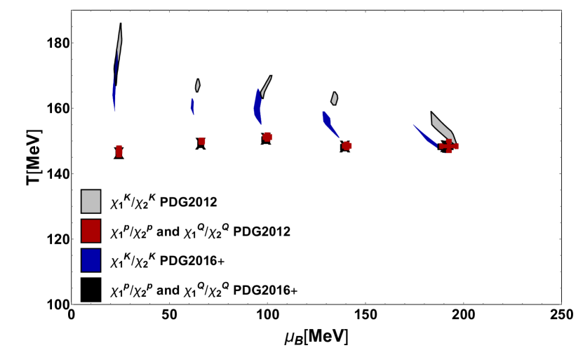
Figure 4: (Color online) Comparison of freeze-out parameters obtained via a combined fit of net-proton and net-electric charge with those obtained from the net-kaon fluctuations following the analysis from Ref. Bellwied et al. (2019) with different particle lists.

The results for the light and kaon freeze-out with the PDG2016+ list are shown in Fig. 4 with black points and blue shapes, respectively. We can see that, as in the analysis with the PDG2012 list from Refs. Alba et al. (2014); Bellwied et al. (2019), there is a separation of the net-kaon from the light particle freeze-out temperature at the higher collision energies (lower $\mu_{B}$) that decreases as the collision energy decreases. With the inclusion of more resonances in the HRG model, the freeze-out temperature for the net-kaons is decreased, while the light hadron freeze-out is mostly unchanged. However, the gap between the two freeze-out temperatures is not closed, and the resulting temperatures are compatible with the ones obtained in the previous Section with the analysis of fits in the double freeze-out scenario.

VII Conclusions

In this paper we explored the effects that including additional, not-well-established hadronic resonances in the PDG lists, as well as a combination of the latter with predicted (but not yet measured) Quark Model states, has on the extracted freeze-out parameters in heavy-ion collisions. In Ref. Bazavov et al. (2014) it was suggested that the addition of missing strange states could possibly explain the tension between proton and multi-strange hadrons production at the LHC. An alternative picture was proposed in Ref. Bellwied et al. (2013) wherein strange hadrons freeze-out at a higher temperature than the light ones, which is due to the higher hadronization temperature of strange particles compared to light particles. We explore this alternative picture here.

For the first time in this paper, we systematically explore the effect of enlarged hadronic resonance spectra – along with their decay properties – on thermal fits, and find that this tension is not resolved. Especially at the LHC, the separation between strange and light freeze-out is extremely pronounced. At RHIC the separation is smaller, and is almost resolved when states from the Quark Model are included, although it is important to remember that certainly too many strange states are predicted by these calculations, as was shown in Ref. Alba et al. (2017). From thermal fits based on the most realistic particle list PDG2016+, we estimate the light chemical freeze-out temperature to be $T_{L}\sim 141-144$ MeV and the strange chemical freeze-out temperature to be $T_{S}\sim 163-167$ MeV at the LHC, and $T_{L}\sim 148-158$ MeV and $T_{S}\sim 155-161$ MeV at RHIC. Generally, the light chemical freeze-out temperature appears to be consistent with the net-p and net-Q results (within error bars), while the strange temperature is consistent with the one obtained from net-K fluctuations.

Finally, we note that in other works Steinheimer et al. (2013); Noronha-Hostler and Greiner (2014b, a) it was suggested the a dynamical scenario could explain the proton to pion puzzle at the LHC. The inclusion of the additional states in such a scenario is left for a future work. Generally, we find hints of two separate chemical freeze-out temperatures, but smaller error bars in the experimental data would be needed before a definitive answer can be given.

Appendix A Graphs

In this Appendix we show a comparison of the yields and ratios to experimental data. The four figures (Figs. 5-8) show the four different particle list fits to yields and ratios at the LHC and RHIC, both in the single (red lines) and double (blue dotted lines) freeze-out scenarios. In the former, $\Lambda$’s and $\Omega$’s tend to be under-predicted by thermal fits while protons tend to be over-predicted. The use of two separate freeze-out temperatures helps to alleviate this tension and tends to achieve a better overall fit of the data. The inclusion of more resonances does not solve the tension in the single freeze-out scenario, as discussed above.

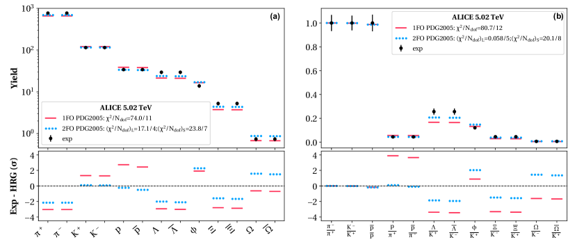
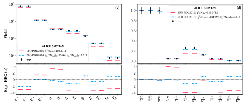
Figure 5: Color online: ALICE PbPb $\sqrt{s_{NN}}=5.02$ TeV data for particle yields (left) and ratios (right) in $0-10\%$ collisions, in comparison to HRG model calculations with the PDG2005 (upper) and PDG2016 (lower); deviations in units of experimental errors $\sigma$ are shown below each panel.

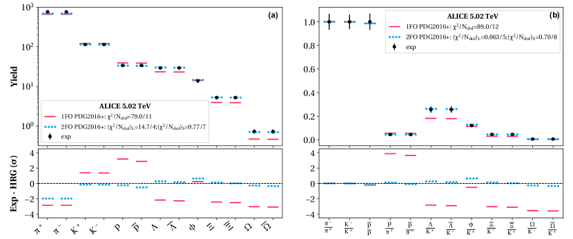
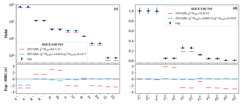
Figure 6: Color online: ALICE PbPb $\sqrt{s_{NN}}=5.02$ TeV data for particle yields (left) and ratios (right) in $0-10\%$ collisions, in comparison to HRG model calculations with the PDG2016+ (upper) and QM (lower) lists; deviations in units of experimental errors $\sigma$ are shown below each panel.

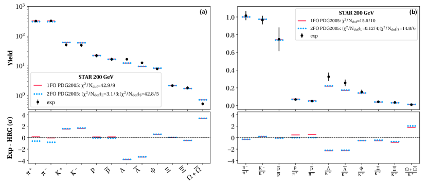
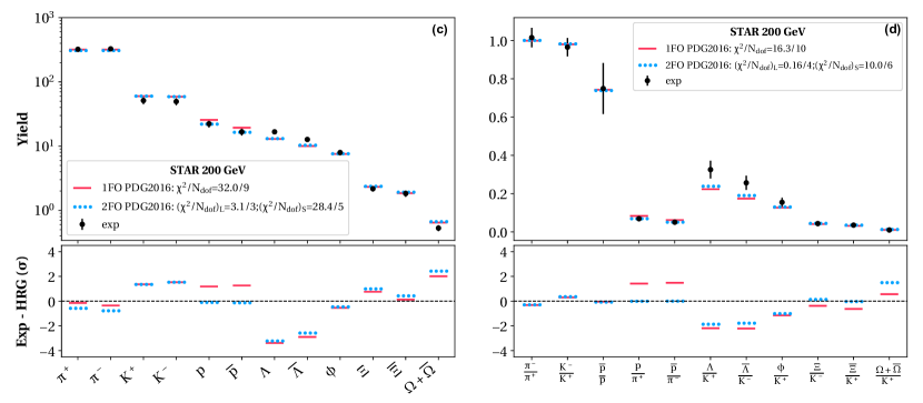
Figure 7: Color online: STAR AuAu $\sqrt{s_{NN}}=200$ GeV data for particle yields (left) and ratios (right) in $0-5\%$ collisions, in comparison to HRG model calculations with the PDG2005 (upper) and PDG2016 (lower); deviations in units of experimental errors $\sigma$ are shown below each panel.

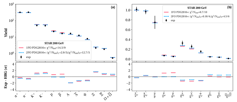
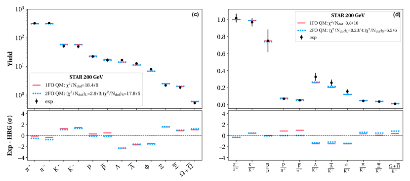
Figure 8: Color online: STAR AuAu $\sqrt{s_{NN}}=200$ GeV data for particle yields (left) and ratios (right) in $0-5\%$ collisions, in comparison to HRG model calculations with the PDG2016+ (upper) and QM (lower); deviations in units of experimental errors $\sigma$ are shown below each panel.

References

- Tanabashi et al. (2018) M. Tanabashi et al. (Particle Data Group), Phys. Rev. D98, 030001 (2018).
- Capstick and Isgur (1986) S. Capstick and N. Isgur, Proceedings, International Conference on Hadron Spectroscopy: College Park, Maryland, April 20-22, 1985, Phys. Rev. D34, 2809 (1986), [AIP Conf. Proc.132,267(1985)].
- Ebert et al. (2009) D. Ebert, R. N. Faustov, and V. O. Galkin, Phys. Rev. D79, 114029 (2009), arXiv:0903.5183 [hep-ph] .
- Cabibbo and Parisi (1975) N. Cabibbo and G. Parisi, Phys. Lett. 59B, 67 (1975).
- Hagedorn (1965) R. Hagedorn, Nuovo Cim. Suppl. 3, 147 (1965).
- Noronha-Hostler et al. (2010a) J. Noronha-Hostler, M. Beitel, C. Greiner, and I. Shovkovy, Phys. Rev. C81, 054909 (2010a), arXiv:0909.2908 [nucl-th] .
- Majumder and Muller (2010) A. Majumder and B. Muller, Phys. Rev. Lett. 105, 252002 (2010), arXiv:1008.1747 [hep-ph] .
- Noronha-Hostler et al. (2012) J. Noronha-Hostler, J. Noronha, and C. Greiner, Phys. Rev. C86, 024913 (2012), arXiv:1206.5138 [nucl-th] .
- Abelev et al. (2014) B. B. Abelev et al. (ALICE), Phys. Lett. B728, 216 (2014), [Erratum: Phys. Lett.B734,409(2014)], arXiv:1307.5543 [nucl-ex] .
- Adam et al. (2017) J. Adam et al. (ALICE), Nature Phys. 13, 535 (2017), arXiv:1606.07424 [nucl-ex] .
- Bellini (2019) F. Bellini (ALICE), Proceedings, 27th International Conference on Ultrarelativistic Nucleus-Nucleus Collisions (Quark Matter 2018): Venice, Italy, May 14-19, 2018, Nucl. Phys. A982, 427 (2019), arXiv:1808.05823 [nucl-ex] .
- Bellwied et al. (2019) R. Bellwied, J. Noronha-Hostler, P. Parotto, I. Portillo Vazquez, C. Ratti, and J. M. Stafford, Phys. Rev. C99, 034912 (2019), arXiv:1805.00088 [hep-ph] .
- Bluhm and Nahrgang (2019) M. Bluhm and M. Nahrgang, Eur. Phys. J. C79, 155 (2019), arXiv:1806.04499 [nucl-th] .
- Bellwied et al. (2020) R. Bellwied, S. Borsanyi, Z. Fodor, J. N. Guenther, J. Noronha-Hostler, P. Parotto, A. Pasztor, C. Ratti, and J. M. Stafford, Phys. Rev. D 101, 034506 (2020), arXiv:1910.14592 [hep-lat] .
- Bellwied et al. (2013) R. Bellwied, S. Borsanyi, Z. Fodor, S. D. Katz, and C. Ratti, Phys. Rev. Lett. 111, 202302 (2013), arXiv:1305.6297 [hep-lat] .
- Bazavov et al. (2014) A. Bazavov et al., Phys. Rev. Lett. 113, 072001 (2014), arXiv:1404.6511 [hep-lat] .
- Noronha-Hostler and Greiner (2014a) J. Noronha-Hostler and C. Greiner, (2014a), arXiv:1405.7298 [nucl-th] .
- Noronha-Hostler and Greiner (2014b) J. Noronha-Hostler and C. Greiner, Proceedings, 24th International Conference on Ultra-Relativistic Nucleus-Nucleus Collisions (Quark Matter 2014): Darmstadt, Germany, May 19-24, 2014, Nucl. Phys. A931, 1108 (2014b), arXiv:1408.0761 [nucl-th] .
- Rapp and Shuryak (2001) R. Rapp and E. V. Shuryak, Phys. Rev. Lett. 86, 2980 (2001), arXiv:hep-ph/0008326 [hep-ph] .
- Steinheimer et al. (2013) J. Steinheimer, J. Aichelin, and M. Bleicher, Phys. Rev. Lett. 110, 042501 (2013), arXiv:1203.5302 [nucl-th] .
- Aarts et al. (2019) G. Aarts, C. Allton, D. De Boni, and B. Jäger, Phys. Rev. D99, 074503 (2019), arXiv:1812.07393 [hep-lat] .
- Lo et al. (2018) P. M. Lo, B. Friman, K. Redlich, and C. Sasaki, Phys. Lett. B778, 454 (2018), arXiv:1710.02711 [hep-ph] .
- Andronic et al. (2019) A. Andronic, P. Braun-Munzinger, B. Friman, P. M. Lo, K. Redlich, and J. Stachel, Phys. Lett. B792, 304 (2019), arXiv:1808.03102 [hep-ph] .
- Alba et al. (2017) P. Alba et al., Phys. Rev. D96, 034517 (2017), arXiv:1702.01113 [hep-lat] .
- Noronha-Hostler et al. (2009) J. Noronha-Hostler, J. Noronha, and C. Greiner, Phys. Rev. Lett. 103, 172302 (2009), arXiv:0811.1571 [nucl-th] .
- Rais et al. (2019) J. Rais, K. Gallmeister, and C. Greiner, (2019), arXiv:1909.04522 [hep-ph] .
- Noronha-Hostler et al. (2014) J. Noronha-Hostler, J. Noronha, G. S. Denicol, R. P. G. Andrade, F. Grassi, and C. Greiner, Phys. Rev. C89, 054904 (2014), arXiv:1302.7038 [nucl-th] .
- Alba et al. (2018) P. Alba, V. Mantovani Sarti, J. Noronha, J. Noronha-Hostler, P. Parotto, I. Portillo Vazquez, and C. Ratti, Phys. Rev. C 98, 034909 (2018), arXiv:1711.05207 [nucl-th] .
- Noronha-Hostler et al. (2010b) J. Noronha-Hostler, H. Ahmad, J. Noronha, and C. Greiner, Phys. Rev. C82, 024913 (2010b), arXiv:0906.3960 [nucl-th] .
- Devetak et al. (2019) D. Devetak, A. Dubla, S. Floerchinger, E. Grossi, S. Masciocchi, A. Mazeliauskas, and I. Selyuzhenkov, (2019), arXiv:1909.10485 [hep-ph] .
- Chatterjee et al. (2013) S. Chatterjee, R. M. Godbole, and S. Gupta, Phys. Lett. B727, 554 (2013), arXiv:1306.2006 [nucl-th] .
- Chatterjee et al. (2017) S. Chatterjee, D. Mishra, B. Mohanty, and S. Samanta, Phys. Rev. C96, 054907 (2017), arXiv:1708.08152 [nucl-th] .
- (33) http://nsmn1.uh.edu/cratti/decays.html.
- Eidelman et al. (2004) S. Eidelman et al. (Particle Data Group), Phys. Lett. B592, 1 (2004).
- Patrignani et al. (2016) C. Patrignani et al. (Particle Data Group), Chin. Phys. C40, 100001 (2016).
- Dashen et al. (1969) R. Dashen, S.-K. Ma, and H. J. Bernstein, Phys. Rev. 187, 345 (1969).
- Venugopalan and Prakash (1992) R. Venugopalan and M. Prakash, Nucl. Phys. A546, 718 (1992).
- Alba et al. (2014) P. Alba, W. Alberico, R. Bellwied, M. Bluhm, V. Mantovani Sarti, M. Nahrgang, and C. Ratti, Phys. Lett. B738, 305 (2014), arXiv:1403.4903 [hep-ph] .
- Alba et al. (2015) P. Alba, R. Bellwied, M. Bluhm, V. Mantovani Sarti, M. Nahrgang, and C. Ratti, Phys. Rev. C92, 064910 (2015), arXiv:1504.03262 [hep-ph] .
- Poberezhnyuk et al. (2019) R. Poberezhnyuk, V. Vovchenko, A. Motornenko, M. I. Gorenstein, and H. Stoecker, Phys. Rev. C100, 054904 (2019), arXiv:1906.01954 [hep-ph] .
- Karsch and Redlich (2011) F. Karsch and K. Redlich, Phys. Lett. B695, 136 (2011), arXiv:1007.2581 [hep-ph] .
- Garg et al. (2013) P. Garg, D. K. Mishra, P. K. Netrakanti, B. Mohanty, A. K. Mohanty, B. K. Singh, and N. Xu, Phys. Lett. B726, 691 (2013), arXiv:1304.7133 [nucl-ex] .
- Fu (2013) J. Fu, Physics Letters B 722, 144 (2013).
- Borsanyi et al. (2013) S. Borsanyi, Z. Fodor, S. D. Katz, S. Krieg, C. Ratti, and K. K. Szabo, Phys. Rev. Lett. 111, 062005 (2013), arXiv:1305.5161 [hep-lat] .
- Borsanyi et al. (2014) S. Borsanyi, Z. Fodor, S. D. Katz, S. Krieg, C. Ratti, and K. K. Szabo, Phys. Rev. Lett. 113, 052301 (2014), arXiv:1403.4576 [hep-lat] .
- Becattini et al. (2006) F. Becattini, J. Manninen, and M. Gazdzicki, Phys. Rev. C73, 044905 (2006), arXiv:hep-ph/0511092 [hep-ph] .
- Becattini et al. (2013) F. Becattini, M. Bleicher, T. Kollegger, T. Schuster, J. Steinheimer, and R. Stock, Phys. Rev. Lett. 111, 082302 (2013), arXiv:1212.2431 [nucl-th] .
- Cleymans et al. (2006) J. Cleymans, H. Oeschler, K. Redlich, and S. Wheaton, Phys. Rev. C73, 034905 (2006), arXiv:hep-ph/0511094 [hep-ph] .
- Torrieri and Rafelski (2007) G. Torrieri and J. Rafelski, Phys. Rev. C75, 024902 (2007), arXiv:nucl-th/0608061 [nucl-th] .
- Andronic et al. (2011) A. Andronic, P. Braun-Munzinger, K. Redlich, and J. Stachel, Quark matter. Proceedings, 22nd International Conference on Ultra-Relativistic Nucleus-Nucleus Collisions, Quark Matter 2011, Annecy, France, May 23-28, 2011, J. Phys. G38, 124081 (2011), arXiv:1106.6321 [nucl-th] .
- Braun-Munzinger et al. (2004) P. Braun-Munzinger, K. Redlich, and J. Stachel, Quark-Gluon Plasma 3, 491 (2004), arXiv:nucl-th/0304013 .
- Andronic et al. (2006) A. Andronic, P. Braun-Munzinger, and J. Stachel, Nucl. Phys. A772, 167 (2006), arXiv:nucl-th/0511071 [nucl-th] .
- Bhattacharyya et al. (2019) S. Bhattacharyya, D. Biswas, S. K. Ghosh, R. Ray, and P. Singha, Phys. Rev. D100, 054037 (2019), arXiv:1904.00959 [nucl-th] .
- Bhattacharyya et al. (2020) S. Bhattacharyya, D. Biswas, S. K. Ghosh, R. Ray, and P. Singha, Phys. Rev. D101, 054002 (2020), arXiv:1911.04828 [hep-ph] .
- Abelev et al. (2009) B. I. Abelev et al. (STAR), Phys. Rev. C79, 034909 (2009), arXiv:0808.2041 [nucl-ex] .
- Adams et al. (2007) J. Adams et al. (STAR), Phys. Rev. Lett. 98, 062301 (2007), arXiv:nucl-ex/0606014 [nucl-ex] .
- Adamczyk et al. (2017) L. Adamczyk et al. (STAR), Phys. Rev. C96, 044904 (2017), arXiv:1701.07065 [nucl-ex] .
- Cleymans et al. (2005) J. Cleymans, B. Kampfer, M. Kaneta, S. Wheaton, and N. Xu, Phys. Rev. C 71, 054901 (2005), arXiv:hep-ph/0409071 .
- Abelev et al. (2013a) B. Abelev et al. (ALICE), Phys. Rev. C88, 044910 (2013a), arXiv:1303.0737 [hep-ex] .
- Abelev et al. (2013b) B. B. Abelev et al. (ALICE), Phys. Rev. Lett. 111, 222301 (2013b), arXiv:1307.5530 [nucl-ex] .
- Abelev et al. (2015) B. B. Abelev et al. (ALICE), Phys. Rev. C91, 024609 (2015), arXiv:1404.0495 [nucl-ex] .
- Andronic et al. (2018) A. Andronic, P. Braun-Munzinger, K. Redlich, and J. Stachel, Nature 561, 321 (2018), arXiv:1710.09425 [nucl-th] .
- Vovchenko and Stoecker (2019) V. Vovchenko and H. Stoecker, Comput. Phys. Commun. 244, 295 (2019), arXiv:1901.05249 [nucl-th] .
- Andronic et al. (2013) A. Andronic, P. Braun-Munzinger, K. Redlich, and J. Stachel, Proceedings, 23rd International Conference on Ultrarelativistic Nucleus-Nucleus Collisions : Quark Matter 2012 (QM 2012): Washington, DC, USA, August 13-18, 2012, Nucl. Phys. A904-905, 535c (2013), arXiv:1210.7724 [nucl-th] .
- Bellwied et al. (2015) R. Bellwied, S. Borsanyi, Z. Fodor, J. Günther, S. D. Katz, C. Ratti, and K. K. Szabo, Phys. Lett. B751, 559 (2015), arXiv:1507.07510 [hep-lat] .
- Bazavov et al. (2017) A. Bazavov et al. (HotQCD), Phys. Rev. D96, 074510 (2017), arXiv:1708.04897 [hep-lat] .
- Adam et al. (2020) J. Adam et al. (STAR), (2020), arXiv:2001.06419 [nucl-ex] .
- Koch (2010) V. Koch, “Hadronic Fluctuations and Correlations,” in Relativistic Heavy Ion Physics, Springer, Heidelberg, edited by R. Stock (2010) pp. 626–652, arXiv:0810.2520 [nucl-th] .
- Gunther et al. (2017) J. Gunther, R. Bellwied, S. Borsanyi, Z. Fodor, S. D. Katz, A. Pasztor, and C. Ratti, Proceedings, 12th Conference on Quark Confinement and the Hadron Spectrum (Confinement XII): Thessaloniki, Greece, EPJ Web Conf. 137, 07008 (2017), arXiv:1607.02493 [hep-lat] .
- Adamczyk et al. (2014a) L. Adamczyk et al. (STAR), Phys. Rev. Lett. 112, 032302 (2014a), arXiv:1309.5681 [nucl-ex] .
- Adamczyk et al. (2014b) L. Adamczyk et al. (STAR), Phys. Rev. Lett. 113, 092301 (2014b), arXiv:1402.1558 [nucl-ex] .
- Adamczyk et al. (2018) L. Adamczyk et al. (STAR), Phys. Lett. B785, 551 (2018), arXiv:1709.00773 [nucl-ex] .
- Kitazawa and Asakawa (2012a) M. Kitazawa and M. Asakawa, Phys. Rev. C85, 021901 (2012a), arXiv:1107.2755 [nucl-th] .
- Kitazawa and Asakawa (2012b) M. Kitazawa and M. Asakawa, Phys. Rev. C86, 024904 (2012b), [Erratum: Phys. Rev.C86,069902(2012)], arXiv:1205.3292 [nucl-th] .