ConQUR: Mitigating Delusional Bias in Deep Q-learning

Abstract

Delusional bias is a fundamental source of error in approximate Q-learning. To date, the only techniques that explicitly address delusion require comprehensive search using tabular value estimates. In this paper, we develop efficient methods to mitigate delusional bias by training Q-approximators with labels that are “consistent” with the underlying greedy policy class. We introduce a simple penalization scheme that encourages Q-labels used across training batches to remain (jointly) consistent with the expressible policy class. We also propose a search framework that allows multiple Q-approximators to be generated and tracked, thus mitigating the effect of premature (implicit) policy commitments. Experimental results demonstrate that these methods can improve the performance of Q-learning in a variety of Atari games, sometimes dramatically.

1 Introduction

Q-learning (Watkins & Dayan, 1992; Sutton & Barto, 2018) lies at the heart of many of the recent successes of deep reinforcement learning (RL) (Mnih et al., 2015; Silver et al., 2016), with recent advancements (e.g., van Hasselt (2010); Bellemare et al. (2017); Wang et al. (2016); Hessel et al. (2017)) helping to make it among the most widely used methods in applied RL. Despite these successes, many properties of Q-learning are poorly understood, and it is challenging to successfully apply deep Q-learning in practice. Various modifications have been proposed to improve convergence or approximation error (Gordon, 1995, 1999; Szepesvári & Smart, 2004; Melo & Ribeiro, 2007; Maei et al., 2010; Munos et al., 2016); but it remains difficult to reliably attain both robustness and scalability.

Recently, Lu et al. (2018) identified a source of error in Q-learning with function approximation known as delusional bias. This bias arises because Q-learning updates the value of state-action pairs using estimates of (sampled) successor-state values that can be mutually inconsistent given the policy class induced by the approximator. This can result in unbounded approximation error, divergence, policy cycling, and other undesirable behavior. To handle delusion, the authors propose a policy-consistent backup operator that maintains multiple Q-value estimates organized into information sets. Each information set has its own backed-up Q-values and corresponding “policy commitments” responsible for inducing these values. Systematic management of these sets ensures that only consistent choices of maximizing actions are used to update Q-values. All potential solutions are tracked to prevent premature convergence on specific policy commitments. Unfortunately, the proposed algorithms use tabular representations of Q-functions, so while this establishes foundations for delusional bias, the function approximator is used neither for generalization nor to manage the size of the state/action space. Consequently, this approach is not scalable to practical RL problems.

In this work, we develop ConQUR (CONsistent Q-Update Regression), a general framework for integrating policy-consistent backups with regression-based function approximation for Q-learning and for managing the search through the space of possible regressors (i.e., information sets). With suitable search heuristics, the proposed framework provides a computationally effective means for minimizing the effects of delusional bias, while scaling to practical problems.

Our main contributions are as follows. First, we define novel augmentations of Q-regression to increase the degree of policy consistency across training batches. Since testing exact consistency is expensive, we introduce an efficient soft-consistency penalty that promotes consistency of labels with earlier policy commitments. Second, using information-set structure (Lu et al., 2018), we define a search space over Q-regressors to explore multiple sets of policy commitments. Third, we propose heuristics to guide the search, critical given the combinatorial nature of information sets. Finally, experimental results on the Atari suite (Bellemare et al., 2013) demonstrate that ConQUR can add (sometimes dramatic) improvements to Q-learning. These results further show that delusion does emerge in practical applications of Q-learning. We also show that straightforward consistency penalization on its own (i.e., without search) can improve both standard and double Q-learning.

2 Background

We assume a discounted, infinite horizon Markov decision process (MDP), $\mathbf{M}=(\mathcal{S},A,P,p_{0},R,\gamma)$. The state space $\mathcal{S}$ can reflect both discrete and continuous features, but we take the action space $A$ to be finite (and practically enumerable). We consider Q-learning with a function approximator $Q_{\theta}$ to learn an (approximately) optimal Q-function (Watkins, 1989; Sutton & Barto, 2018), drawn from some approximation class parameterized by $\Theta$ (e.g., the weights of a neural network). When the approximator is a deep network, we generically refer to this as DQN, the method at the heart of many RL successes (Mnih et al., 2015; Silver et al., 2016).

For online Q-learning, at a transition $s,a,r,s^{\prime}$, the Q-update is given by:

$$\theta\leftarrow\theta+\alpha\Big{(}r+\gamma\max_{a^{\prime}\in A}Q_{\theta}(s^{\prime},a^{\prime})-Q_{\theta}(s,a)\Big{)}\nabla_{\theta}Q_{\theta}(s,a).$$ (1)

Batch versions of Q-learning are similar, but fit a regressor repeatedly to batches of training examples (Ernst et al., 2005; Riedmiller, 2005), and are usually more data efficient and stable than online Q-learning. Batch methods use a sequence of (possibly randomized) data batches $D_{1},\ldots,D_{T}$ to produce a sequence of regressors $Q_{\theta_{1}},\ldots,Q_{\theta_{T}}=Q_{\theta}$, estimating the Q-function. For each $(s,a,r,s^{\prime})\in D_{k}$, we use a prior estimator $Q_{\theta_{k-1}}$ to bootstrap the Q-label $q=r+\gamma\max_{a^{\prime}}Q_{\theta_{k-1}}(s^{\prime},a^{\prime})$. We then fit $Q_{\theta_{k}}$ to this data using a regression procedure with a suitable loss function. Once trained, the (implicit) induced policy $\pi_{\theta}$ is the greedy policy w.r.t. $Q_{\theta}$, i.e., $\pi_{\theta}(s)=\operatorname*{arg\!max}_{a\in A}Q_{\theta}(s,a)$. Let $\mathcal{F}(\Theta)$ (resp., $G(\Theta)$) be the class of expressible Q-functions (resp., greedy policies).

Intuitively, delusional bias occurs whenever a backed-up value estimate is derived from action choices that are not (jointly) realizable in $G(\Theta)$ (Lu et al., 2018). Standard Q-updates back up values for each $(s,a)$ pair by independently choosing maximizing actions at the corresponding next states $s^{\prime}$. However, such updates may be “inconsistent” under approximation: if no policy in $G(\Theta)$ can jointly express all past action choices, backed up values may not be realizable by any expressible policy. Lu et al. (2018) show that delusion can manifest itself with several undesirable consequences (e.g., divergence). Most critically, it can prevent Q-learning from learning the optimal representable policy in $G(\Theta)$. To address this, they propose a non-delusional policy consistent Q-learning (PCQL) algorithm that provably eliminates delusion. We refer to the original paper for details, but review the main concepts.

The first key concept is that of policy consistency. For any $S\subseteq\mathcal{S}$, an action assignment $\sigma_{S}:S\rightarrow A$ associates an action $\sigma(s)$ with each $s\in S$. We say $\sigma$ is policy consistent if there is a greedy policy $\pi\in G(\Theta)$ s.t. $\pi(s)=\sigma(s)$ for all $s\in S$. We sometimes equate a set $\mathit{SA}$ of state-action pairs with the implied assignment $\pi(s)=a$ for all $(s,a)\in\mathit{SA}$. If $\mathit{SA}$ contains multiple pairs with the same state $s$, but different actions $a$, it is a multi-assignment (we use the term “assignment” when there is no risk of confusion).

In (batch) Q-learning, each new regressor uses training labels generated by assuming maximizing actions (under the prior regressor) are taken at its successor states. Let $\sigma_{k}$ be the collection of states and corresponding maximizing actions used to generate labels for regressor $Q_{\theta_{k}}$ (assume it is policy consistent). Suppose we train $Q_{\theta_{k}}$ by bootstrapping on $Q_{\theta_{k-1}}$. Now consider a training sample $(s,a,r,s^{\prime})$. Q-learning generates label $r+\gamma\max_{a^{\prime}}Q_{\theta_{k-1}}(s^{\prime},a^{\prime})$ for input $(s,a)$. Notice, however, that taking action $a^{*}=\operatorname*{arg\!max}_{a^{\prime}}Q_{\theta_{k}}(s^{\prime},a^{\prime})$ at $s^{\prime}$ may not be policy consistent with $\sigma_{k}$. Thus Q-learning will estimate a value for $(s,a)$ assuming execution of a policy that cannot be realized given the approximator. PCQL prevents this by ensuring that any assignment used to generate labels is consistent with earlier assignments. This means Q-labels will often not be generated using maximizing actions w.r.t. the prior regressor.

The second key concept is that of information sets. One will generally not be able to use maximizing actions to generate labels, so tradeoffs can be made when deciding which actions to assign to different states. Indeed, even if it is feasible to assign a maximizing action $a$ to state $s$ early in training, say at batch $k$, since it may prevent assigning a maximizing $a^{\prime}$ to $s^{\prime}$ later, say batch $k+\ell$, we may want to use a different assignment to $s$ to give more flexibility to maximize at other states later. PCQL does not anticipate the tradeoffs—rather it maintains multiple information sets, each corresponding to a different assignment to the states seen in the training data this far. Each gives rise to a different Q-function estimate, resulting in multiple hypotheses. At the end of training, the best hypothesis is that with maximum expected value w.r.t. an initial state distribution.

PCQL provides strong convergence guarantees, but it is a tabular algorithm: the function approximator restricts the policy class, but is not used to generalize Q-values. Furthermore, its theoretical guarantees come at a cost: it uses exact policy consistency tests—tractable for linear approximators, but impractical for large problems and DQN; and it maintains all consistent assignments. As a result, PCQL cannot be used for large RL problems of the type tackled by DQN.

3 The ConQUR Framework

We develop the ConQUR framework to provide a practical approach to reducing delusion in Q-learning, specifically addressing the limitations of PCQL identified above. ConQUR consists of three main components: a practical soft-constraint penalty that promotes policy consistency; a search space to structure the search over multiple regressors (information sets, action assignments); and heuristic search schemes (expansion, scoring) to find good Q-regressors.

3.1 Preliminaries

We assume a set of training data consisting of quadruples $(s,a,r,s^{\prime})$, divided into (possibly non-disjoint) batches $D_{1},\ldots,D_{T}$ for training. This perspective is quite general: online RL corresponds to $|D_{i}|=1$; offline batch training (with sufficiently exploratory data) corresponds to a single batch (i.e., $T=1$); and online or batch methods with replay are realized when the $D_{i}$ are generated by sampling some data source with replacement.

For any batch $D$, let $\chi(D)=\{s^{\prime}:(s,a,r,s^{\prime})\in D\}$ be the set of successor states of $D$. An action assignment $\sigma_{D}$ for $D$ is an assignment (or multi-assignment) from $\chi(D)$ to $A$, dictating which action $\sigma_{D}(s^{\prime})$ is considered “maximum” when generating a Q-label for pair $(s,a)$; i.e., $(s,a)$ is assigned training label $r+\gamma Q(s^{\prime},\sigma(s^{\prime}))$ rather than $r+\gamma\max_{a^{\prime}\in A}Q(s^{\prime},a^{\prime})$. The set of all such assignments $\Sigma(D)=A^{\chi(D)}$ grows exponentially with $|D|$.

Given a Q-function parameterization $\Theta$, we say $\sigma_{D}$ is $\Theta$-consistent (w.r.t. $D$) if there is some $\theta\in\Theta$ s.t. $\pi_{\theta}(s^{\prime})=\sigma(s^{\prime})$ for all $s^{\prime}\in\chi(D)$. This is simple policy consistency, but with notation that emphasizes the policy class. Let $\Sigma_{\Theta}(D)$ denote the set of all $\Theta$-consistent assignments over $D$. The union $\sigma_{1}\cup\sigma_{2}$ of two assignments (over $D_{1},D_{2}$, resp.) is defined in the usual way.

3.2 Consistency Penalization

Enforcing strict $\Theta$-consistency as regressors $\theta_{1},\theta_{2},\ldots,\theta_{T}$ are generated is computationally challenging. Suppose the assignments $\sigma_{1},\ldots,\sigma_{k-1}$, used to generate labels for $D_{1},\ldots D_{k-1}$, are jointly $\Theta$-consistent (let $\sigma_{\leq k-1}$ denote their multi-set union). Maintaining $\Theta$-consistency when generating $\theta_{k}$ imposes two requirements. First, one must generate an assignment $\sigma_{k}$ over $D_{k}$ s.t. $\sigma_{\leq k-1}\cup\sigma_{k}$ is consistent. Even testing assignment consistency can be problematic: for linear approximators this is a linear feasibility program (Lu et al., 2018) whose constraint set grows linearly with $|D_{1}\cup\ldots\cup D_{k}|$. For DNNs, this is a complex, more expensive polynomial program. Second, the regressor $\theta_{k}$ should itself be consistent with $\sigma_{\leq k-1}\cup\sigma_{k}$. This too imposes a severe burden on regression optimization: in the linear case, it is a constrained least-squares problem (solvable, e.g., as a quadratic program); while with DNNs, it can be solved, say, using a more involved projected SGD. However, the sheer number of constraints makes this impractical.

Rather than enforcing consistency, we propose a simple, computationally tractable scheme that “encourages” it: a penalty term that can be incorporated into the regression itself. Specifically, we add a penalty function to the usual squared loss to encourage updates of the Q-regressors to be consistent with the underlying information set, i.e., the prior action assignments used to generate its labels.

When constructing $\theta_{k}$, let $D_{\leq k}=\cup\{D_{j}:j\leq k\}$, and $\sigma\in\Sigma_{\Theta}({D_{\leq k}})$ be the collective assignment used to generate labels for all prior regressors (including $\theta_{k}$ itself). The multiset of pairs $B=\{(s^{\prime},\sigma(s^{\prime}))|s^{\prime}\in\chi(D_{\leq k})\}$, is called a consistency buffer. The assignment need not be consistent (as we elaborate below), nor does regressor $\theta_{k}$ need to be consistent with $\sigma$. Instead, we use the following soft consistency penalty when constructing $\theta_{k}$:

$$C_{\theta}(s^{\prime},a) =\sum_{a^{\prime}\in A}[Q_{\theta}(s^{\prime},a^{\prime})-Q_{\theta}(s^{\prime},a)]_{+},$$ (2)

$$C_{\theta}(B) =\sum_{(s^{\prime},\sigma(s^{\prime}))\in B}C_{\theta}(s^{\prime},\sigma(s^{\prime})),$$ (3)

where $[x]_{+}=\max(0,x)$. This penalizes Q-values of actions at state $s$ that are larger than that of action $\sigma(s)$. Notice $\sigma$ is $\Theta$-consistent iff $\min_{\theta\in\Theta}C_{\theta}(B)=0$. We add this penalty into our regression loss for batch $D_{k}$:

$$L_{\theta}(D_{k},B)=\sum_{(s,a,r,s^{\prime})\in D_{k}}\Big{[}r+\gamma Q_{\theta_{k-1}}(s^{\prime},\sigma(s^{\prime}))-\\ Q_{\theta}(s,a)\Big{]}^{2}+\lambda C_{\theta}(B).$$ (4)

Here $Q_{\theta_{k}}$ is the prior estimator on which labels are bootstrapped (other regressors may be used). The penalty effectively acts as a “regularizer” on the squared Bellman error, where $\lambda$ controls the degree of penalization, allowing a tradeoff between Bellman error and consistency with the assignment used to generate labels. It thus promotes consistency without incurring the expense of enforcing strict consistency. It is straightforward to replace the classic Q-learning update (1) with one using our consistency penalty:

$$\theta_{k}\leftarrow\theta_{k-1}+\sum_{(s,a,r,s^{\prime})\in D_{k}}\alpha\Big{[}r+\gamma Q_{\theta_{k-1}}(s^{\prime},\sigma(s^{\prime}))\\ -Q_{\theta}(s,a)\Big{]}\nabla_{\theta}Q_{\theta}(s,a)+\alpha\lambda\nabla_{\theta}C_{\theta}(B)\Bigr{\rvert}_{\theta=\theta_{k-1}}.$$ (5)

This scheme is quite general. First, it is agnostic as to how the prior action assignments are made (e.g., standard maximization w.r.t. the prior regressor as in DQN, Double DQN (DDQN) (Hasselt et al., 2016), or other variants). It can also be used in conjunction with a search through alternate assignments (see below).

Second, the consistency buffer $B$ may be populated in a variety of ways. Including all max-action choices from all past training batches promotes full consistency. However, this may be too constraining since action choices early in training are generally informed by inaccurate value estimates. $B$ may be implemented to focus only on more recent data (e.g., with a sliding recency window, weight decay, or subsampling); and the degree of recency bias may adapt during training (e.g., becoming more inclusive as training proceeds and the Q-function converges). Reducing the size of $B$ also has computational benefits. We discuss other ways of promoting consistency in Sec. 5.

The proposed consistency penalty resembles the temporal-consistency loss of Pohlen et al. (2018), but our aims are very different. Their temporal consistency notion penalizes changes in a next state’s Q-estimate over all actions, whereas we discourage inconsistencies in the greedy policy induced by the Q-estimator, regardless of the actual estimated values.

3.3 The Search Space

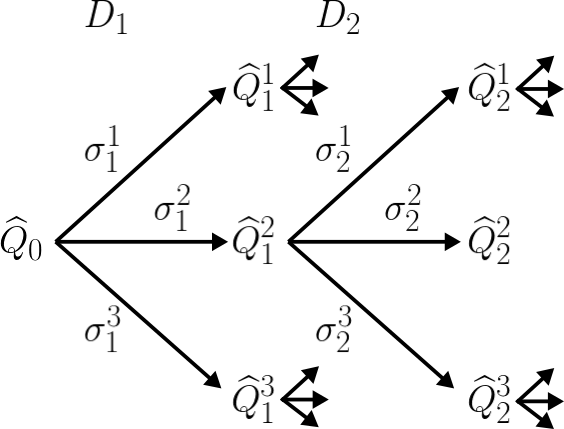
Figure 1: A generic search tree.

Ensuring optimality requires that PCQL track all $\Theta$-consistent assignments. While the set of such assignments has polynomial size (Lu et al., 2018), it is impractical to track in realistic problems. As such, in ConQUR we recast information set tracking as a search problem and propose several strategies for managing the search process. We begin by defining the search space and discussing its properties. We discuss search procedures in Sec. 3.4.

As above, assume training data is divided into batches $D_{1},\ldots,D_{T}$ and we have some initial Q-function estimate $\theta_{0}$ (for bootstrapping $D_{1}$’s labels). The regressor $\theta_{k}$ for $D_{k}$ can, in principle, be trained with labels generated by any assignment $\sigma\in\Sigma_{\Theta}(D_{k})$ of actions to its successor states $\chi(D_{k})$, not necessarily maximizing actions w.r.t. $\theta_{k-1}$. Each $\sigma$ gives rise to a different updated Q-estimator $\theta_{k}$. There are several restrictions we can place on “reasonable” $\sigma$-candidates: (i) $\sigma$ is $\Theta$-consistent; (ii) $\sigma$ is jointly $\Theta$-consistent with all $\sigma_{j}$, for $j<k$, used to construct the prior regressors on which we bootstrap $\theta_{k-1}$; (iii) $\sigma$ is not dominated by any $\sigma^{\prime}\in\Sigma_{\Theta}(D_{k})$, where we say $\sigma^{\prime}$ dominates $\sigma$ if $Q_{\theta_{k-1}}(s^{\prime},\sigma^{\prime}(s^{\prime}))\geq Q_{\theta_{k-1}}(s^{\prime},\sigma(s^{\prime}))$ for all $s^{\prime}\in\chi(D)$, and this inequality is strict for at least one $s^{\prime}$. Conditions (i) and (ii) are the strict consistency requirements of PCQL. We relax these below as discussed in Sec. 3.2. Condition (iii) is inappropriate in general, since we may add additional assignments (e.g., to new data) that render all non-dominated assignments inconsistent, requiring that we revert to some dominated assignment.

This gives us a generic search space for finding policy-consistent, delusion-free Q-function (see Fig. 1). Each node $n^{i}_{k}$ at depth $k$ in the search tree is associated with a regressor $\theta^{i}_{k}$ defining $Q_{\theta^{i}_{k}}$ and assignment $\sigma^{i}_{k}$ that justifies the labels used to train $\theta^{i}_{k}$ ($\sigma^{i}_{k}$ can be viewed as an information set). The root $n_{0}$ is based on an initial $\theta_{0}$, and has an empty assignment $\sigma_{0}$. Nodes at level $k$ of the tree are defined as follows. For each node $n_{k-1}^{i}$ at level $k-1$—with regressor $\theta_{k-1}^{i}$ and $\Theta$-consistent assignment $\sigma_{k-1}^{i}$—we have one child $n_{k}^{j}$ for each $\sigma_{k}^{j}\in\Sigma_{\Theta}(D_{k})$ such that $\sigma_{k-1}^{i}\cup\sigma_{k}^{j}$ is $\Theta$-consistent. Node $n_{k}^{j}$’s assignment is $\sigma_{k-1}^{i}\cup\sigma_{k}^{j}$, and its regressor $\theta_{k}^{i}$ is trained using the data set:

$$\{(s,a)\mapsto r+\gamma Q_{\theta_{k-1}^{i}}(s^{\prime},\sigma_{k}^{j}(s^{\prime}))\,:\,(s,a,r,s^{\prime})\in D_{k}\}.$$

The entire search space constructed in this fashion to a maximum depth of $T$. See Appendix B, Algorithm 1 for pseudocode of a simple depth-first recursive specification.

The exponential branching factor in this search tree would appear to make complete search intractable; however, since we only allow $\Theta$-consistent “collective” assignments we can bound the size of the tree—it is polynomial in the VC-dimension of the approximator.

Theorem 1.

The number of nodes in the search tree is no more than $O(nm\cdot[\binom{m}{2}n]^{\operatorname*{\mathsf{VCDim}}(\mathcal{G})})$ where $\operatorname*{\mathsf{VCDim}}(\cdot)$ is the VC-dimension (Vapnik, 1998) of a set of boolean-valued functions, and $\mathcal{G}$ is the set of boolean functions defining all feasible greedy policies under $\Theta$: $\mathcal{G}=\{g_{\theta}(s,a,a^{\prime}):={\mathbf{1}}[f_{\theta}(s,a)-f_{\theta}(s,a^{\prime})>0],\forall s,a\neq a^{\prime}~{}|~{}\theta\in\Theta\}.$

A linear approximator with a fixed set of $d$ features induces a policy-indicator function class $\mathcal{G}$ with VC-dimension $d$, making the search tree polynomial in the size of the MDP. Similarly, a fixed ReLU DNN architecture with $W$ weights and $L$ layers has VC-dimension of size $O(WL\log W)$ again rendering the tree polynomially sized.

Even with this bound, navigating the search space exhaustively is generally impractical. Instead, various search methods can be used to explore the space, with the aim of reaching a “high quality” regressor at some leaf of the tree.

3.4 Search Heuristics

Even with the bound in Thm. 1, traversing the search space exhaustively is generally impractical. Moreover, as discussed above, enforcing consistency when generating the children of a node, and their regressors, may be intractable. Instead, various search methods can be used to explore the space, with the aim of reaching a “high quality” regressor at some (depth $T$) leaf of the tree. We outline three primary considerations in the search process: child generation, node evaluation or scoring, and the search procedure.

Generating children. Given node $n^{i}_{k-1}$, there are, in principle, exponentially many action assignments, or children, $\Sigma_{\Theta}(D_{k})$ (though Thm. 1 limits this if we enforce consistency). Thus, we develop heuristics for generating a small set of children, driven by three primary factors.

The first factor is a preference for generating high-value assignments. To accurately reflect the intent of (sampled) Bellman backups, we prefer to assign actions to state $s^{\prime}\in\chi(D_{k})$ with larger predicted Q-values i.e., a preference for $a$ over $a^{\prime}$ if ${Q}_{\theta_{k-1}^{j}}(s^{\prime},a)>{Q}_{\theta_{k-1}^{j}}(s^{\prime},a^{\prime})$. However, since the maximizing assignment may be $\Theta$-inconsistent (in isolation, jointly with the parent information set, or with future assignments), candidate children should merely have higher probability of a high-value assignment. Second, we need to ensure diversity of assignments among the children. Policy commitments at stage $k$ constrain the assignments at subsequent stages. In many search procedures (e.g., beam search), we avoid backtracking, so we want the stage-$k$ commitments to offer flexibility in later stages. The third factor is the degree to which we enforce consistency.

There are several ways to generate high-value assignments. We focus on one natural technique: sampling action assignments using a Boltzmann distribution. Let $\sigma$ be the assignment of some node (parent) at level $k-1$ in the tree. We generate an assignment $\sigma_{k}$ for $D_{k}$ as follows. Assume some permutation $s_{1}^{\prime},\ldots,s^{\prime}_{|D_{k}|}$ of $\chi(D_{k})$. For each $s^{\prime}_{i}$ in turn, we sample $a_{i}$ with probability proportional to $e^{Q_{\theta_{k-1}}(s^{\prime}_{i},a_{i})/\tau}$. This can be done without regard to consistency, in which case we use the consistency penalty when constructing the regressor $\theta_{k}$ for this child to “encourage” consistency rather than enforce it. If we want strict consistency, we can use rejection sampling without replacement to ensure $a_{i}$ is consistent with $\sigma^{j}_{k-1}\cup\sigma_{\leq i-1}$ (we can also use a subset of $\sigma^{j}_{k-1}$ as a less restrictive consistency buffer). The temperature parameter $\tau$ controls the degree to which we focus on maximizing assignments versus diverse, random assignments. While sampling gives some diversity, this procedure biases selection of high-value actions to states that occur early in the permutation. To ensure further diversity, we use a new random permutation for each child.

Scoring children. Once the children of some expanded node are generated, we must assess the quality of each child to decide which new nodes to expand. One possiblity is to use the average Q-label (overall, or weighted using an initial distribution), Bellman error, or loss incurred by the regressor. However, care must be taken when comparing nodes at different depths of the tree. Since deeper nodes have a greater chance to accrue rewards or costs, simple calibration methods can be used. Alternatively, when a simulator is available, rollouts of the induced greedy policy can be used evaluate the node quality. However, rollouts incur considerable computational expense during training relative to the more direct scoring methods.

Search Procedure. Given a method for generating and scoring children, different search procedures can be applied: best-first search, beam search, local search, etc. all fit very naturally within the ConQUR framework. Moreover, hybrid strategies are possible—one we develop below is a variant of beam search in which we generate multiple children only at certain levels of the tree, then do “deep dives” using consistency-penalized Q-regression at the intervening levels. This reduces the size of the search tree considerably and, when managed properly, adds only a constant-factor (proportional to beam size) slowdown to methods like DQN.

3.5 An Instantiation of the ConQUR Framework

We now outline a specific instantiation of the ConQUR framework that effectively navigates the large search spaces that arise in practical RL settings. We describe a heuristic, modified beam-search strategy with backtracking and priority scoring. We outline only key features (see details in Algorithm 2, Appendix B).

Our search process alternates between two phases. In an expansion phase, parent nodes are expanded, generating one or more child nodes with assignments sampled from the Boltzmann distribution. For each child, we create target Q-labels, then optimize its regressor using consistency-penalized Bellman error Eq. 4, foregoing strict policy consistency. In a dive phase, each parent generates one child, whose action assignment is given by standard max-action selection w.r.t. the parent’s regressor. No diversity is considered but we continue to use consistency-penalized regression.

From the root, the search begins with an expansion phase to create $c$ children—$c$ is the splitting factor. Each child inherits its parent’s consistency buffer to which we add the new assignments used for that child’s Q-labels. To limit the tree size, we track a subset of the children (the frontier), selected using some scoring function. We select the top $\ell$-nodes for expansion, proceed to a dive phase and iterate.

We consider backtracking strategies that return to unexpanded nodes at shallower depths of the tree below.

3.6 Related Work

Other work has considered multiple hypothesis tracking in RL. One direct approach uses ensembling, with multiple Q-approximators updated in parallel (Faußer & Schwenker, 2015; Osband et al., 2016; Anschel et al., 2017) and combined to reduce instability and variance. Population-based methods, inspired by evolutionary search, are also used. Conti et al. (2018) combine novelty search and quality diversity to improve hypothesis diversity and quality. Khadka & Tumer (2018) augment an off-policy RL method with diversified population information derived from an evolutionary algorithm. These techniques do not target a specific weaknesses of Q-learning, such as delusion.

4 Empirical Results

We assess the performance of ConQUR using the Atari test suite (Bellemare et al., 2013). Since ConQUR directly tackles delusion, any performance improvement over Q-learning baselines strongly suggests the presence of delusional bias in the baselines in these domains. We first assess the impact of our consistency penalty in isolation (without search), treating it as a “regularizer” that promotes consistency with both DQN and DDQN. We then test our modified beam search to assess the full power of ConQUR. We do not directly compare ConQUR to policy gradient or actor-critic methods—which for some Atari games offer state-of-the-art performance (Schrittwieser et al., 2019; Kapturowski et al., 2020)—because our aim with ConQUR is to improve the performance of (widely used) Q-learning-based algorithms.

4.1 Consistency Penalization

We first study the effects of augmenting both DQN and DDQN with soft-policy consistency in isolation. We train models using an open-source implementation of DQN and DDQN, using default hyperparameters (Guadarrama et al., 2018) . We refer to the consistency-augmented algorithms as $\mathsf{DQN}{(\lambda)}$ and $\mathsf{DDQN}{(\lambda)}$, respectively, where $\lambda$ is the penalty weight (see Eq. 4). When $\lambda=0$, these correspond to DQN and DDQN themselves. This policy-consistency augmentation is lightweight and can be applied readily to any regression-based Q-learning method. Since we do not use search (i.e., do not track multiple hypotheses), these experiments use a small consistency buffer drawn only from the current data batch by sampling from the replay buffer—this prevents getting “trapped” by premature policy commitments. No diversity is used to generate action assignments—standard action maximization is used.

We evaluate $\mathsf{DQN}{(\lambda)}$ and $\mathsf{DDQN}{(\lambda)}$ for $\lambda\in\{0.25,0.5,1,1.5,2\}$ on 19 Atari games. In training, $\lambda$ is initialized at $0$ and annealed to the desired value to avoid premature commitment to poor assignments. Unsurprisingly, the best $\lambda$ tends to differ across games depending on the extent of delusional bias. Despite this, $\lambda=0.5$ works well across all games tested. Fig. 2 illustrates the effect of increasing $\lambda$ on two games. In Gravitar, it results in better performance in both $\mathsf{DQN}{}$ and $\mathsf{DDQN}{}$, while in SpaceInvaders, $\lambda=0.5$ improves both baselines, but relative performance degrades at $\lambda=2$.

We also compare performance on each game for each $\lambda$ value, as well as using the best $\lambda_{\textrm{best}}$ (see Fig. 8, Table 3 in Appendix C.4). $\mathsf{DQN}{(\lambda_{\text{best}})}$ and $\mathsf{DDQN}{(\lambda_{\text{best}})}$ outperform their “potentially delusional” counterparts in all but 3 and 2 games, respectively. In 9 games, both $\mathsf{DQN}{(\lambda_{\text{best}})}$ and $\mathsf{DDQN}{(\lambda_{\text{best}})}$ beat both baselines. With a fixed $\lambda=0.5$, $\mathsf{DQN}{(\lambda)}$ and $\mathsf{DDQN}{(\lambda)}$ each beat their respective baseline in 11 games. These results suggest that consistency penalization—independent of the general ConQUR model—can improve the performance of DQN and DDQN by addressing delusional bias. Moreover, promoting policy consistency appears to have a different effect on learning than double Q-learning, which addresses maximization bias. Indeed, consistency penalization, when applied to $\mathsf{DQN}{}$, achieves greater gains than $\mathsf{DDQN}{}$ in 15 games. Finally, in 9 games $\mathsf{DDQN}{(\lambda)}$ improves unaugmented $\mathsf{DQN}{(\lambda)}$. Further experiment details and results can be found in Appendix C.

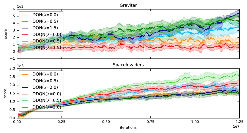
Figure 2: Varying penalization $\lambda$ (no search procedure).

4.2 Full ConQUR

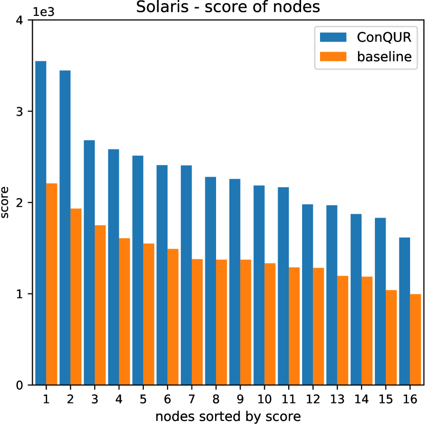
Figure 3: Policy value (game scores) of nodes, sorted.

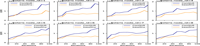
Figure 4: Training curves of 8 sorted nodes.

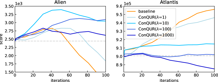
Figure 5: Performance effects of varying $\lambda$.

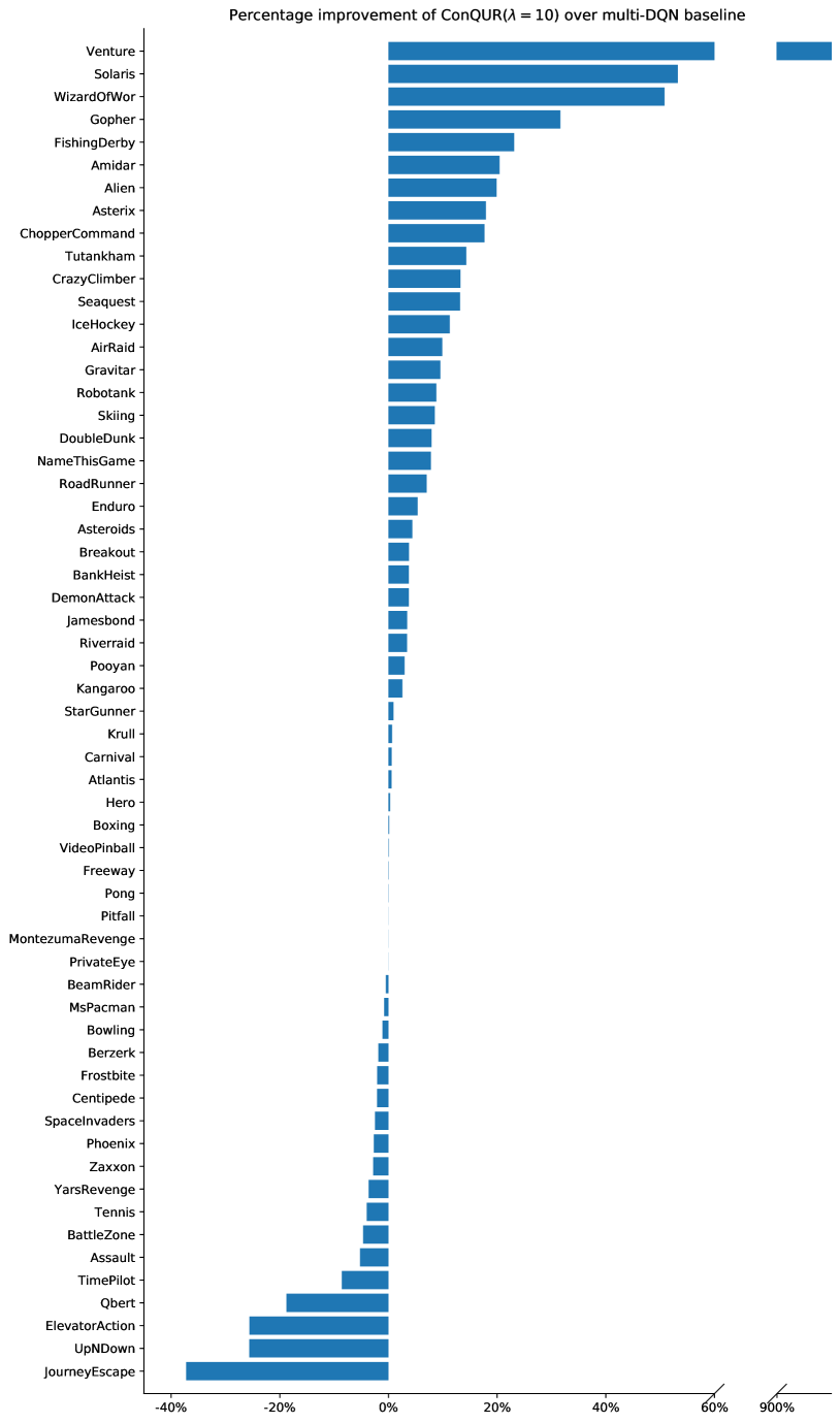
Figure 6: Improvements of ConQUR($\lambda=10$) over multi-DQN baseline on all 59 games. A frontier $F=16$ nodes was used.

We test the full ConQUR framework using our modified beam search (Sec. 3.5) on the full suite of 59 Atari games. Rather than training a full Q-network using ConQUR, we leverage pre-trained networks from the Dopamine package (Castro et al., 2018), and use ConQUR to learn final layer weights, i.e., a new “linear approximator” w.r.t. the learned feature representation. We do this for two reasons. First, this allows us to test whether delusional bias occurs in practice. By freezing the learned representation, any improvements offered by ConQUR when learning a linear Q-function over those same features provides direct evidence that (a) delusion is present in the original trained baselines, and (b) ConQUR does in fact mitigate its impact (without relying on novel feature discovery). Second, from a practical point of view, this “linear tuning” approach offers a relatively inexpensive way to apply our methodology in practice. By bootstrapping a model trained in standard fashion and extracting performance gains with a relatively small amount of additional training (e.g., linear tuning requires many fewer training samples, as our results show), we can offset the cost of the ConQUR search process itself.

We use DQN-networks with the same architecture as in Mnih et al. (2015), trained on 200M frames as our baseline. We use ConQUR to retrain only the last (fully connected) layer (freezing other layers), which can be viewed as a linear Q-approximator over the features learned by the CNN. We train Q-regressors in ConQUR using only 4M additional frames. We use a splitting factor of $c=4$ and frontier size 16. The dive phase is always of length nine (i.e., nine batches of data), giving an expansion phase every ten iterations. Regressors are trained using soft-policy consistency (Eq. 4), with the consistency buffer comprising all prior action assignments. We run ConQUR with $\lambda\in\{1,10\}$ and select the best performing policy. We use larger $\lambda$ values than in Sec. 4.1 since full ConQUR maintains multiple Q-regressors and can “discard” poor performers. This allows more aggressive consistency enforcement—in the extreme, with exhaustive search and $\lambda\to\infty$, ConQUR behaves like PCQL, finding a near-optimal greedy policy. See Appendix D for further details (e.g., hyperparameters) and results.

We first test two approaches to scoring nodes: (i) policy evaluation using rollouts; and (ii) scoring using the loss function (Bellman error with soft consistency). Results on a small selection of games are shown in Table 1. While rollouts, unsurprisingly, tend to induce better-performing policies, consistent-Bellman scoring is competitive. Since the latter much less computationally intense, and does not require a simulator (or otherwise sampling the environment), we use it throughout our remaining experiments.

We next compare ConQUR with the value of the pre-trained DQN. We also evaluate a “multi-DQN” baseline that trains multiple DQNs independently, warm-starting from the same pre-trained DQN. It uses the same number of frontier nodes as ConQUR, and is trained identically to ConQUR, but uses direct Bellman error (no consistency penalty). This gives DQN the same advantage of multiple-hypothesis tracking as ConQUR (without its policy consistency).

	Rollouts	Bellman + Consistency Penalty
BattleZone	33796.30	32618.18
BeamRider	9914.00	10341.20
Boxing	83.34	83.03
Breakout	379.21	393.00
MsPacman	5947.78	5365.06
Seaquest	2848.04	3000.78
SpaceInvader	3442.31	3632.25
StarGunner	55800.00	56695.35
Zaxxon	11064.00	10473.08

Table 1: Results of ConQUR with 8 nodes (split 2) on 9 games: comparing loss-based node scoring with scoring using rollouts.

We test on 59 games. ConQUR with frontier size 16 and expansion factor 4 and splitting factor 4 (16-4-4) with backtracking (as described in the Appendix D) results in significant improvements over the pre-trained DQN, with an average score improvement of 189%. The only games without improvement are Montezuma’s Revenge, Tennis, Freeway, Pong, PrivateEye and BankHeist. This demonstrates that, even when simply retraining the last layer of a highly tuned DQN network, removing delusional bias frequently improves policy performance significantly. ConQUR exploits the reduced parameterization to obtain these gains with only 4M frames of training data. A half-dozen games have outsized improvements over pre-trained DQN, including Venture (35 times greater value), ElevatorAction (23 times), Tutankham (5 times) and Solaris (5 times).

We found that $\lambda=10$ provided the best performance across all games. Fig. 6 shows the percentage improvement of ConQUR($\lambda=10$) over the multi-DQN baseline for all 59 games. The improvement is defined as $(s_{C}-s_{B})/|s_{B}|$ where $s_{C}$ and $s_{B}$ are the average scores (over 5 runs) of the policy generated by ConQUR and that by the multi-DQN baseline (16 nodes), respectively. Compared to this stronger baseline, ConQUR wins by a margin of at least 10% in 16 games, while 19 games see improvements of 1–10%, 16 games show little effect ($\pm 1$%) and 8 games show a decline of greater than 1%. Tables of complete results and figures of training curves (all games) appears in Appendix D.3, Table 4 and Fig. 11.

Figs. 3 and 4 (smoothed, best frontier node) show node policy values and training curves, respectively, for Solaris. When examining nodes ranked by their policy value (Fig. 3), we see that nodes of any given rank generated by ConQUR dominate their by multi-DQN (baseline) counterparts: the three highest-ranked nodes exceed their baseline counterparts by 18%, 13% and 15%, respectively, while the remaining nodes show improvements of roughly 11–12%. Fig. 5 (smoothed, best frontier node) shows the effect of varying $\lambda$. In Alien, increasing $\lambda$ from 1 to 10 improves performance, but performance starts to decline for higher $\lambda$ (we tested both 100 and 1000). This is similar to patterns observed in Sec. 4.1 and represents a trade-off between emphasizing consistency and not over-committing to action assignments. In Atlantis, stronger penalization tends to degrade performance. In fact, the stronger the penalization, the worse the performance.

5 Concluding Remarks

We have introduced ConQUR, a framework for mitigating delusional bias in various forms of Q-learning that relaxes some of the strict assumptions of exact delusion-free algorithms like PCQL to ensure scalability. Its main components are a search procedure used to maintain diverse, promising Q-regressors (and corresponding information sets); and a consistency penalty that encourages “maximizing” actions to be consistent with the approximator class. ConQUR embodies elements of both value-based and policy-based RL: it can be viewed as using partial policy constraints to bias the Q- value estimator, and as a means of using candidate value functions to bias the search through policy space. Empirically, we find that ConQUR can improve the quality of existing approximators by removing delusional bias. Moreover, the consistency penalty applied on its own, in either DQN or DDQN, can improve policy quality.

There are many directions for future research. Other methods for nudging regressors to be policy-consistent include exact consistency (i.e., constrained regression), other regularization schemes that push the regressor to fall within the information set, etc. Further exploration of search, child-generation, and node-scoring strategies should be examined within ConQUR. Our (full) experiments should also be extended beyond those that warm-start from a DQN model. We believe our methods can be extended to both continuous actions and soft max-action policies. We are also interested in the potential connection between maintaining multiple “hypotheses” (i.e., Q-regressors) and notions in distributional RL (Bellemare et al., 2017).

Appendix A An Example of Delusional Bias

We describe an example, taken directly from (Lu et al., 2018), to show concretely how delusional bias causes problems for Q-learning with function approximation. The MDP in Fig. 7 illustrates the phenomenon: Lu et al. (2018) use a linear approximator over a specific set of features in this MDP to show that:

1. No $\pi\in G(\Theta)$ can express the optimal (unconstrained) policy (which requires taking $a_{2}$ at each state);

2. The optimal feasible policy in $G(\Theta)$ takes $a_{1}$ at $s_{1}$ and $a_{2}$ at $s_{4}$ (achieving a value of $0.5$).

3. Online Q-learning (Eq. 1) with data generated using an $\varepsilon$-greedy behavior policy must converge to a fixed point (under a range of rewards and discounts) corresponding to a “compromise” admissible policy which takes $a_{1}$ at both $s_{1}$ and $s_{4}$ (value of $0.3$).

Q-learning fails to find a reasonable fixed-point because of delusion. Consider the backups at $(s_{2},a_{2})$ and $(s_{3},a_{2})$. Suppose $\hat{\theta}$ assigns a “high” value to $(s_{3},a_{2})$, so that $Q_{\hat{\theta}}(s_{3},a_{2})>Q_{\hat{\theta}}(s_{3},a_{1})$ as required by $\pi_{\theta^{\ast}}$. They show that any such $\hat{\theta}$ also accords a “high” value to $(s_{2},a_{2})$. But $Q_{\hat{\theta}}(s_{2},a_{2})>Q_{\hat{\theta}}(s_{2},a_{1})$ is inconsistent the first requirement. As such, any update that makes the Q-value of $(s_{2},a_{2})$ higher undercuts the justification for it to be higher (i.e., makes the “max” value of its successor state $(s_{3},a_{2})$ lower). This occurs not due to approximation error, but the inability of Q-learning to find the value of the optimal representable policy.

Figure 7: A simple MDP (Lu et al., 2018).

Appendix B Algorithms

The pseudocode of (depth-first) version of the ConQUR search framework is listed in Algorithm 1.

Algorithm 1 ConQUR Search (Generic, depth-first)

0:  Data sets $D_{k},D_{k+1},\ldots D_{T}$; regressor $\hat{Q}_{k-1}$; and assignment $\sigma$ over $D_{\leq k-1}=\cup_{1\leq j\leq k-1}D_{j}$ reflecting prior data; policy class $\Theta$.

1:  Let $\Sigma_{\Theta,\sigma}=\{\sigma_{k}\in\Sigma_{\Theta}(D_{j}):\sigma_{k}\cup\sigma\textrm{ is consistent}\}$

2:  for all $\sigma_{k}^{j}\in\Sigma_{\Theta,\sigma}$ do

3:     Training set $S\leftarrow\{\}$

4:     for all $(s,a,r,s^{\prime})\in D_{k}$ do

5:        $q\leftarrow r+\gamma\hat{Q}_{k-1}(s^{\prime},\sigma_{k}^{j}(s^{\prime}))$

6:        $S\leftarrow S\cup\{((s,a),q)\}$

7:     end for

8:     Train $\hat{Q}^{j}_{k}$ using training set $S$

9:     if $k=T$ then

10:        Return $\hat{Q}^{j}_{k}$ // terminate

11:     else

12:        Return Search($D_{k+1},\ldots D_{T};\,\hat{Q}^{j}_{k};\,\sigma_{k}^{j}\cup\sigma;\,\Theta$) // recurse

13:     end if

14:  end for

As discussed in Sec. 3.5, a more specific instantiation of the ConQUR algorithm is listed in Algorithm 2.

Algorithm 2 Modified Beam Search Instantiation of ConQUR Algorithm

0:  Search control parameters: $m$, $\ell$, $c$, $d$, $T$

1:  Maintain list of data batches $D_{1},...,D_{k}$, initialized empty

2:  Maintain candidate pool $P$ of at most $m$ nodes, initialized $P=\{n_{0}\}$

3:  Maintain frontier list $F$ of $\ell^{c}$ nodes

4:  Maintain for each node $n^{i}_{k}$ a regressor $\theta^{i}_{k}$ and an ancestor assignment $\sigma^{i}_{k}$

5:  for  each search level $k\leq T$  do

6:     Find top scoring node $n^{1}\in P$

7:     Use $\varepsilon$-greedy policy extracted from $Q_{\theta^{1}}$ to collect next data batch $D_{k}$

8:     if  $k$ is an expansion level  then

9:        Select top $\ell$ scoring nodes $n^{1},...,n^{\ell}\in P$

10:        for  each selected node $n^{i}$  do

11:           Generate $c$ children $n^{i,1},...,n^{i,c}$ using Boltzmann sampling on $D_{k}$ with $Q_{\theta^{i}}$

12:           for  each child $n^{i,j}$  do

13:              Let assignment history $\sigma^{i,j}$ be $\sigma^{i}\cup\{\textit{new assignment}\}$

14:              Determine regressor $\theta^{i,j}$ by applying update (5) from $\theta^{i}$

15:           end for

16:           Score and add child nodes to the candidate pool $P$

17:           Assign frontier nodes to set of child nodes, $F=\{n^{i,j}\}$

18:           if  $|P|>m$  then

19:              evict bottom scoring nodes, keeping top $m$ in $P$

20:           end if

21:        end for

22:     end if

23:     if  $k$ is a refinement (”dive”) level  then

24:        for  each frontier node $n^{i,j}\in F$  do

25:           Update regressor $\theta^{i,j}$ by applying update (5) to $\theta^{i,j}$

26:        end for

27:     end if

28:     Run $d$ ”dive” levels after each expansion level

29:  end for

Appendix C Additional Detail: Effects of Consistency Penalization

C.1 Delusional bias in DQN and DDQN

Both DQN and DDQN uses a delayed version of the $Q$-network $Q_{\theta^{-}}(s^{\prime},a^{\prime})$ for label generation, but in a different way. In DQN, $Q_{\theta^{-}}(s^{\prime},a^{\prime})$ is used for both value estimate and action assignment $\sigma_{\text{DQN}}(s^{\prime})=\operatorname*{arg\!max}_{a^{\prime}}Q_{\theta_{k}}(s^{\prime},a^{\prime})$, whereas in DDQN, $Q_{\theta^{-}}(s^{\prime},a^{\prime})$ is used only for value estimate and the action assignment is computed from the current network $\sigma_{\text{DDQN}}(s^{\prime})=\operatorname*{arg\!max}_{a^{\prime}}Q_{\theta_{k}}(s^{\prime},a^{\prime})$.

With respect to delusional bias, action assignment of DQN is consistent for all batches after the latest network weight transfer, as $\sigma_{\text{DQN}}(s^{\prime})$ is computed from the same $Q_{\theta^{-}}(s^{\prime},a^{\prime})$ network. DDQN, on the other hand, could have very inconsistent assignments, since the action is computed from the current network that is being updated at every step.

C.2 Training Methodology and Hyperparameters

We implement consistency penalty on top of the DQN and DDQN algorithm by modifying the open-source TF-Agents library (Guadarrama et al., 2018). In particular, we modify existing DqnAgent and DdqnAgent by adding a consistency penalty term to the original TD loss.

We use TF-Agents implementation of DQN training on Atari with the default hyperparameters, which are mostly the same as that used in the original DQN paper (Mnih et al., 2015). For conveniece to the reader, some important hyperparameters are listed in Table 2. The reward is clipped between $[-1,1]$ following the original DQN.

Hyper-parameter	Value
Mini-batch size	32
Replay buffer capacity	1 million transitions
Discount factor $\gamma$	0.99
Optimizer	RMSProp
Learning rate	0.00025
Convolution channel	$32,64,64$
Convolution filter size	$(8\times 8),(4\times 4),(3\times 3)$
Convolution stride	4, 2, 1
Fully-connected hidden units	512
Train exploration $\varepsilon_{\text{train}}$	0.01
Eval exploration $\varepsilon_{\text{eval}}$	0.001

Table 2: Hyperparameters for training DQN and DDQN with consistency penalty on Atari.

C.3 Evaluation Methodology

We empirically evaluate our modified DQN and DDQN agents trained with consistency penalty on 15 Atari games. Evaluation is run using the training and evaluation framework for Atari provided in TF-Agents without any modifications.

C.4 Detailed Results

Fig. 8 shows the effects of varying $\lambda$ on both DQN and DDQN. Table 3 summarizes the best penalties for each game and their corresponding scores. Fig. 9 shows the training curves of the best penalization constants. Finally, Fig. 10 shows the training curves for a fixed penalization of $\lambda=0.5$. The datapoints in each plot of the aforementioned figures are obtained by averaging over window size of 30 steps, and within each window, we take the largest policy value (and over $\approx$2–5 multiple runs). This is done to reduce visual clutter.

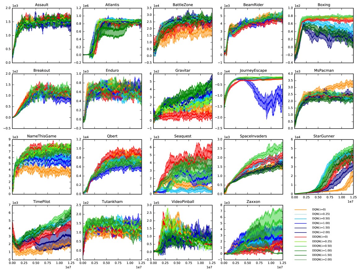
Figure 8: DQN and DDQN training curves for different penalty constant $\lambda$.

	$\mathsf{DQN}{}$	$\lambda_{\text{best}}$	$\mathsf{DQN}{(\lambda_{\text{best}})}$	$\mathsf{DDQN}{}$	$\lambda^{\prime}_{\text{best}}$	$\mathsf{DDQN}{(\lambda^{\prime}_{\text{best}})}$
Assault	2546.56	1.5	3451.07	2770.26	1	2985.74
Atlantis	995460.00	0.5	1003600.00	940080.00	1.5	999680.00
BattleZone	67500.00	2	55257.14	47025.00	2	48947.37
BeamRider	7124.90	0.5	7216.14	5926.59	0.5	6784.97
Boxing	86.76	0.5	90.01	82.80	0.5	91.29
Breakout	220.00	0.5	219.15	214.25	0.5	242.73
Enduro	1206.22	0.5	1430.38	1160.44	1	1287.50
Gravitar	475.00	1.5	685.76	462.94	1.5	679.33
JourneyEscape	-1020.59	0.25	-696.47	-794.71	1	-692.35
MsPacman	4104.59	2	4072.12	3859.64	0.5	4008.91
NameThisGame	7230.71	1	9013.48	9618.18	0.5	10210.00
Qbert	13270.64	0.5	14111.11	13388.92	1	12884.74
Seaquest	5849.80	1	6123.72	12062.50	1	7969.77
SpaceInvaders	2389.22	0.5	2707.83	3007.72	0.5	4080.57
StarGunner	40393.75	0.5	55931.71	55957.89	0.5	60035.90
TimePilot	4205.83	2	7612.50	6654.44	2	7964.10
Tutankham	222.76	1	265.86	243.20	0.25	247.17
VideoPinball	569502.19	0.25	552456.00	509373.50	0.25	562961.50
Zaxxon	5533.33	1	10520.00	7786.00	0.5	10333.33

Table 3: Consistency penalty ablation results on best penalty constants for DQN and DDQN.

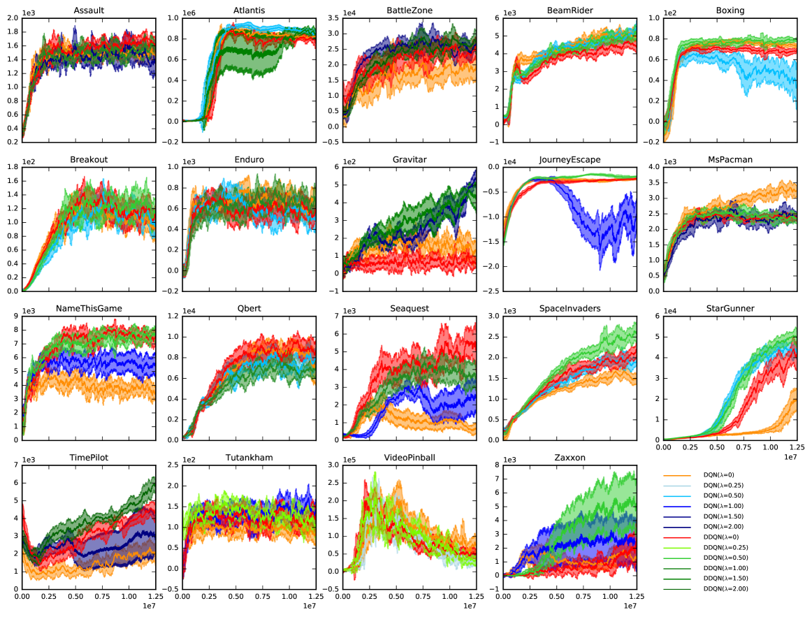
Figure 9: DQN and DDQN training curves for the respective best $\lambda$ and baseline.

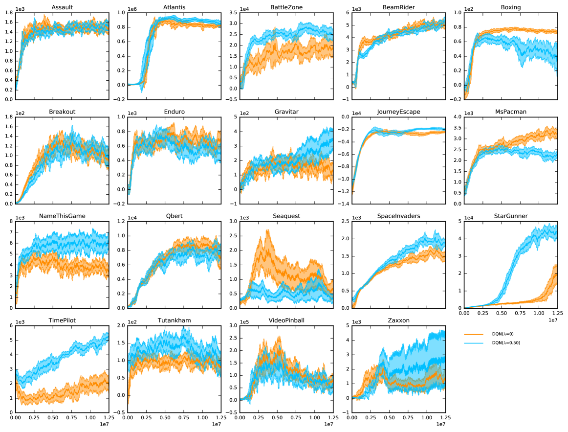
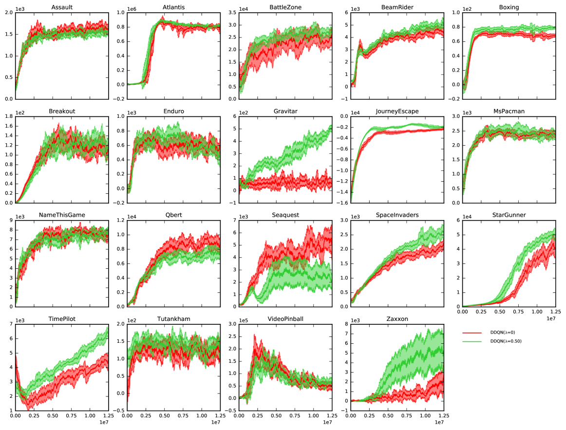
Figure 10: DQN and DDQN training curves for $\lambda=0.5$ and the baseline.

Appendix D Additional Detail: ConQUR Results

Our results use a frontier queue of size ($F$) 16 (these are the top scoring leaf nodes which receive gradient updates and rollout evaluations during training). To generate training batches, we select the best node’s regressor according to our scoring function, from which we generate training samples (transitions) using $\varepsilon$-greedy. Results are reported in Table 4, and training curves in Fig. 11. We used Bellman error plus consistency penalty as our scoring function. During the training process, we also calibrated the scoring to account for the depth difference between the leaf nodes at the frontier versus the leaf nodes in the candidate pool. We calibrated by taking the mean of the difference between scores of the current nodes in the frontier with their parents. We scaled this difference by multiplying with a constant of 2.5.

In our implementation, we initialized our Q-network with a pre-trained DQN. We start with the expansion phase. During this phase, each parent node splits into $l$ children nodes and the Q-labels are generated using action assignments from the Boltzmann sampling procedure, in order to create high quality and diversified children. We start the dive phase until the number of children generated is at least $F$. In particular, with $F=16$ configuration, we performed the expansion phase at the zero-th and first iterations, and then at every tenth iteration starting at iteration 10, then at 20, and so on until ending at iteration 90. All other iterations execute the “dive” phase. For every fifth iteration, Q-labels are generated from action assignments sampled according to the Boltzmann distribution. For all other iterations, Q-labels are generated in the same fashion as the standard Q-learning (taking the max Q-value). The generated Q-labels along with the consistency penalty are then converted into gradient updates that applies to one or more generated children nodes.

D.1 Training Methodology and Hyperparameters

Each iteration consists of 10k transitions sampled from the environment. Our entire training process has 100 iterations which consumes 1M transitions or 4M frames. We used RMSProp as the optimizer with a learning rate of $2.5\times 10^{-6}$. One training iteration has 2.5k gradient updates and we used a batch size of 32. We replace the target network with the online network every fifth iteration and reward is clipped between $[-1,1]$. We use a discount value of $\gamma=0.99$ and $\varepsilon$-greedy with $\varepsilon=0.01$ for exploration. Details of hyper-parameter settings can be found in Table 5, 6.

D.2 Evaluation Methodology

We empirically evaluate our algorithms on 59 Atari games (Bellemare et al., 2013), and followed the evaluation procedure as in Hasselt et al. (2016). We evaluate our agents on every 10-th iteration (and also the initial and first iteration) by suspending our training process. We evaluate on 500k frames, and we cap the length of the episodes for 108k frames. We used $\varepsilon$-greedy as the evaluation policy with $\varepsilon=0.001$. We evaluated our algorithm under the no-op starts regime—in this setting, we insert a random number of “do-nothing” (or no-op) actions (up to 30) at the beginning of each episode.

D.3 Detailed Results

Fig. 11 shows training curves of ConQUR with 16 nodes under different penalization strengths $\lambda\in\{1,10\}$. While each game has its own optimal $\lambda$, in general, we found that $\lambda=10$ gave the best performance for most games. Each plotted step of each training curve (including the baseline) shows the best performing node’s policy value as evaluated with full rollouts. Table 4 shows the summary of the highest policy values achieved for all 59 games for ConQUR and the baseline under 16 nodes. Both the baseline and ConQUR improve overall, but ConQUR’s advantage over the baseline is amplified. These results all use a splitting factor of $c=4$. (We show results with 8 nodes and a splitting factor of 2 below.)

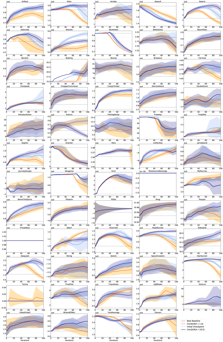
Figure 11: Training curves on 16 nodes with up to 30 no-op starts.

	ConQUR($\lambda_{\text{best}}$) (16 nodes)	Baseline (16 nodes)	Checkpoint
AirRaid	10613.01	9656.21	6916.88
Alien	3253.18	2713.05	2556.64
Amidar	555.75	446.88	203.08
Assault	2007.81	2019.99	1932.55
Asterix	5483.41	4649.52	2373.44
Asteroids	1249.13	1196.56	701.96
Atlantis	958932.00	931416.00	902216.00
BankHeist	1002.59	965.34	872.91
BattleZone	31860.30	32571.80	26559.70
BeamRider	9009.14	9052.38	6344.91
Berzerk	671.95	664.69	525.06
Bowling	38.36	39.79	25.04
Boxing	81.37	81.26	80.89
Breakout	372.31	359.17	286.83
Carnival	4889.19	4860.66	4708.14
Centipede	4025.57	2408.23	758.21
ChopperCommand	7818.22	6643.07	2991.00
CrazyClimber	134974.00	119194.00	63181.14
DemonAttack	11874.80	11445.20	7564.14
DoubleDunk	-14.04	-15.25	-16.66
ElevatorAction	24.67	28.67	0.00
Enduro	879.84	835.11	556.97
FishingDerby	16.28	13.22	6.92
Freeway	32.65	32.63	32.52
Frostbite	289.25	230.29	166.44
Gopher	11959.20	9084.00	4879.02
Gravitar	489.22	446.64	394.46
Hero	20827.00	20765.70	20616.30
IceHockey	-3.15	-3.55	-8.59
Jamesbond	710.78	681.05	624.36
JourneyEscape	902.22	1437.06	-947.18
Kangaroo	11017.65	10743.10	10584.20
Krull	9556.53	9487.49	3998.90
MontezumaRevenge	0.00	0.00	0.00
MsPacman	5444.31	5487.12	4160.50
NameThisGame	9104.40	8445.43	5524.73
Phoenix	5325.33	5430.49	4801.18
Pitfall	0.00	0.00	-4.00
Pong	21.00	21.00	20.95
Pooyan	5898.46	5728.05	4393.09
PrivateEye	100.00	100.00	100.00
Qbert	13812.40	15189.00	8625.88
Riverraid	15895.10	15370.10	11364.90
RoadRunner	50820.40	47481.10	45073.25
Robotank	62.74	57.66	53.08
Seaquest	3046.34	2691.88	1060.77
Skiing	-13638.80	-14908.21	-29897.07
Solaris	1991.33	1202.89	285.46
SpaceInvaders	3556.10	3520.96	2895.30
StarGunner	55679.27	55176.90	51490.60
Tennis	0.00	0.00	0.00
TimePilot	6698.88	7327.71	3806.54
Tutankham	252.51	220.90	36.07
UpNDown	31258.84	34455.20	5956.24
Venture	37.37	3.64	0.00
VideoPinball	423012.59	383105.41	268476.04
WizardOfWor	8154.73	4782.11	2012.24
YarsRevenge	26188.24	26330.31	25000.36
Zaxxon	11723.20	11589.90	5334.44

Table 4: Summary of scores with $\varepsilon$-greedy ($\varepsilon=0.001$) evaluation with up to 30 no-op starts. We ran ConQUR with 16 nodes and with $\lambda\in\{1,10\}$. We report the scores of the best $\lambda_{\text{best}}$ for each game. For most games, $\lambda_{\text{best}}$ is $10$.

Hyperparameters	Description	Value
Dive levels $d$ to run	We run $d$ levels of diving phase after each expansion phase	9
Boltzmann Iteration	Every module this number of iteration/level, Q-labels are generated from Boltzmann distribution in order to create diversified node.	5
Online network target network swap frequency	Iteration (Frequency) at which the online network parameters swap with the target network	5
Evaluation frequency	Iteration (Frequency) at which we perform rollout operation (testing with the environment).	10
Learning Rate	Learning rate for the optimizer.	$2.5\times 10^{-6}$
Optimizer	Optimizer for training the neural network.	RMSprop
Iteration training data transition size	For each iteration, we generate this number of transitions and use it as training data.	10k
Training step frequency	For each iteration, we perform (iteration training data transition size / training step frequency) number of gradient updates.	4
Mini-batch size	Size of the mini batch data used to train the Q-network.	32
$\varepsilon_{\textrm{train}}$	$\varepsilon$-greedy policy for exploration during training.	0.01
$\varepsilon_{\textrm{eval}}$	$\varepsilon$-greedy policy for evaluating Q-regressors.	0.001
Training calibration parameter	Calibration to adjust the difference between the nodes from the candidate pool $m$ which didn’t selected during both the expansion nor the dive phases. The calibration is performed based on the average difference between the frontier nodes and their parents. We denote this difference as $\bigtriangleup$.	$2.5\bigtriangleup$
Temperature $\tau$	Temperature parameter for Boltzmann sampling. Adaptively multiplied or divided by a factor of 1.5 or 4 respectively.	1
Discount factor $\gamma$	Discount factor during the training process.	0.99

Table 5: Common Hyperparameters for ConQUR training and evaluation.

Hyperparameters	Description	Value
Splitting factor $c$	Number of children created from a parent node	4
Candidate pool size $m$	Pool of candidate leaf nodes for selection into the dive or expansion phase	46
Maximum frontier nodes $F$	Maximum number of child leaf nodes for the dive phase	16
Top nodes to expand $l$	Select the top $l$ nodes from the candidate pool for the expansion phase.	4

Table 6: Hyperparameters for ConQUR (16 nodes) training and evaluation.

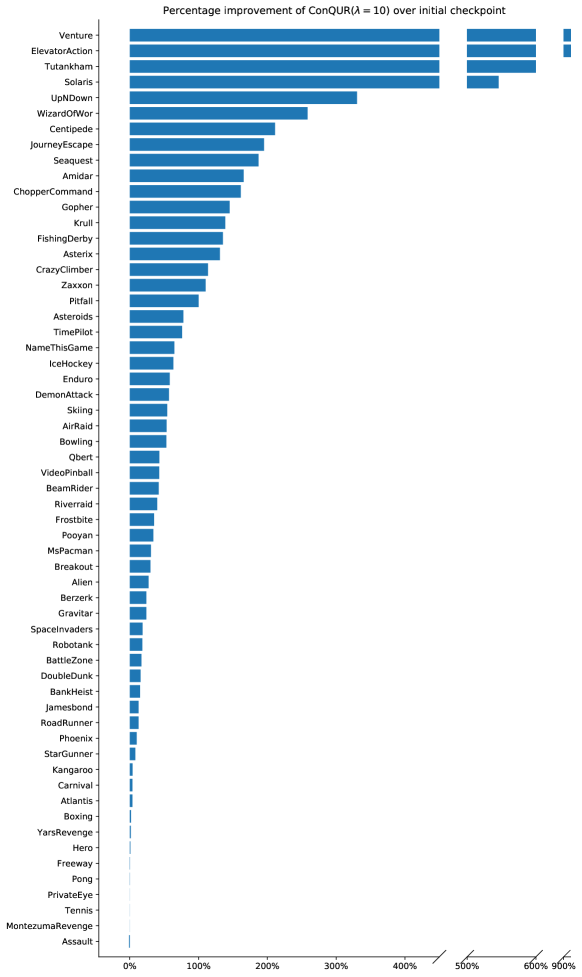
Figure 12: Improvement ConQUR($\lambda=10$) with 16 nodes achieves over the initial checkpoint Q-network.

D.4 Additional Results: ConQUR with 8 Nodes

As an additional study of ConQUR, we present results of the running our method using 8 nodes (rather than the 16 used above), and compare it to a multi-DQN baseline that also uses 8 “nodes” (i.e., 8 separate DQN runs). We use a splitting factor $c=2$ for $\textsc{ConQUR}{}.$ Table 7 shows the average scores for each game using ConQUR and the baseline with 8 nodes. Unsurprisingly, ConQUR with 8 nodes does not perform as well as ConQUR with 16 nodes; but as in the 16-node case, ConQUR outperforms the baseline when each uses 8 nodes. More importantly, the average improvement of $24.5\%$ for ConQUR with 16 nodes over the corresponding baseline exceeds the $19.6\%$ improvement of ConQUR in the 8-node case. This is a strong indication that increasing the number of nodes increases the performance gap relative to the corresponding multi-DQN baseline; this implies that a good search heuristic is critical to effectively navigate the search space (as compared to randomly selected nodes) with a greater number of candidate hypotheses.

	ConQUR($\lambda_{\text{best}}$) (8 nodes)	Baseline (8 nodes)	Checkpoint
AirRaid	10647.80	9050.86	6885.72
Alien	3341.36	3207.5.05	2556.64
Amidar	577.45	573.55	202.74
Assault	1892.02	1976.80	1873.05
Asterix	5026.24	4935.21	2373.44
Asteroids	1194.90	1170.11	704.38
Atlantis	949012.00	932668.00	902216.00
BankHeist	909.61	924.75	871.91
BattleZone	32139.90	30983.10	26558.70
BeamRider	8613.98	8109.63	6397.49
Berzerk	659.64	634.83	524.76
Bowling	30.07	25.29	25.04
Boxing	81.78	81.48	80.29
Breakout	350.11	362.98	286.14
Carnival	4862.30	4800.83	4708.23
Centipede	2747.89	2608.78	757.51
ChopperCommand	7188.25	6737.21	2641.71
CrazyClimber	131675.00	122424.00	63181.11
DemonAttack	11346.20	10947.90	8022.08
DoubleDunk	-13.57	-15.35	-16.66
ElevatorAction	28.00	21.33	0.00
Enduro	849.07	811.58	556.56
FishingDerby	13.34	11.56	7.15
Freeway	32.60	32.60	32.52
Frostbite	296.57	220.81	165.01
Gopher	9999.61	8013.34	4879.13
Gravitar	475.03	480.64	394.46
Hero	20803.60	20774.80	20598.40
IceHockey	-3.23	-4.78	-8.63
Jamesbond	664.98	669.54	626.53
JourneyEscape	-462.64	391.44	-947.18
Kangaroo	10974.00	10733.60	10584.20
Krull	9503.62	9538.22	4039.78
MontezumaRevenge	1.46	0.00	0.00
MsPacman	5066.17	5227.84	4160.50
NameThisGame	9181.30	8410.29	5529.50
Phoenix	5307.46	5227.84	4801.18
Pitfall	0.00	0.00	-4.00
Pong	21.00	20.99	20.95
Pooyan	5778.99	5184.14	4393.09
PrivateEye	100.00	100.00	100.00
Qbert	11953.40	13965.80	8625.88
Riverraid	15614.40	14812.40	11253.30
RoadRunner	49864.80	46302.20	45073.25
Robotank	61.92	56.90	53.08
Seaquest	2647.82	2560.61	1034.83
Skiing	-14058.90	-14079.80	-29896.80
Solaris	1956.24	1182.59	291.70
SpaceInvaders	3436.16	3292.68	2895.30
StarGunner	55479.00	54207.30	51419.60
Tennis	0.00	0.00	0.00
TimePilot	6717.62	6799.19	3806.22
Tutankham	242.03	229.23	36.00
UpNDown	22544.60	23331.20	5956.21
Venture	15.41	1.50	0.00
VideoPinball	382110.59	390540.41	209620.0
WizardOfWor	5750.05	3632.17	2011.77
YarsRevenge	25631.10	25396.70	25319.20
Zaxxon	10751.80	11156.20	5186.01

Table 7: Summary of scores with $\varepsilon$-greedy ($\varepsilon=0.001$) evaluation with up to 30 no-op starts. As a side study, we ran ConQUR with 8 nodes and with $\lambda\in\{1,10\}$. We report the scores of the best $\lambda_{\text{best}}$ for each game. For most games, $\lambda_{\text{best}}$ is $10$. The 8 nodes configuration follows the same as in Table 5, except that $c=2,m=38,F=8,l=2.$

References

- Anschel et al. (2017) Anschel, O., Baram, N., and Shimkin, N. Averaged-dqn: Variance reduction and stabilization for deep reinforcement learning. arXiv:1611.01929, 2017.
- Bellemare et al. (2017) Bellemare, M., Dabney, W., and Munos, R. A distributional perspective on reinforcement learning. In Proceedings of the International Conference on Machine Learning (ICML-17), 2017.
- Bellemare et al. (2013) Bellemare, M. G., Naddaf, Y., Veness, J., and Bowling, M. The arcade learning environment: An evaluation platform for general agents. Journal of Artificial Intelligence Research, 47:253–279, June 2013.
- Castro et al. (2018) Castro, P. S., Moitra, S., Gelada, C., Kumar, S., and Bellemare, M. G. Dopamine: A research framework for deep reinforcement learning. arXiv:1812.06110 [cs.LG], 2018.
- Conti et al. (2018) Conti, E., Madhavan, V., Such, F. P., Lehman, J., Stanley, K. O., and Clune, J. Improving exploration in evolution strategies for deep reinforcement learning via a population of novelty-seeking agents. arXiv:1712.06560, 2018.
- Ernst et al. (2005) Ernst, D., Geurts, P., and Wehenkel, L. Tree-based batch mode reinforcement learning. Journal of Machine Learning Research, 6:503–556, 2005.
- Faußer & Schwenker (2015) Faußer, S. and Schwenker, F. Neural network ensembles in reinforcement learning. Neural Processing Letters, 2015.
- Gordon (1999) Gordon, G. Approximation Solutions to Markov Decision Problems. PhD thesis, Carnegie Mellon University, 1999.
- Gordon (1995) Gordon, G. J. Stable function approximation in dynamic programming. In Proceedings of the Twelfth International Conference on Machine Learning (ICML-95), pp. 261–268, Lake Tahoe, 1995.
- Guadarrama et al. (2018) Guadarrama, S., Korattikara, A., Oscar Ramirez, P. C., Holly, E., Fishman, S., Wang, K., Gonina, E., Wu, N., Harris, C., Vanhoucke, V., and Brevdo, E. TF-Agents: A library for reinforcement learning in tensorflow. https://github.com/tensorflow/agents, 2018. URL https://github.com/tensorflow/agents.
- Hasselt et al. (2016) Hasselt, H. v., Guez, A., and Silver, D. Deep reinforcement learning with double q-learning. In Proceedings of the Thirtieth AAAI Conference on Artificial Intelligence, AAAI’16, pp. 2094–2100. AAAI Press, 2016. URL http://dl.acm.org/citation.cfm?id=3016100.3016191.
- Hessel et al. (2017) Hessel, M., Modayil, J., van Hasselt, H., Schaul, T., Ostrovski, G., Dabney, W., Horgan, D., Piot, B., Azar, M., and Silver, D. Rainbow: Combining improvements in deep reinforcement learning. arXiv:1710.02298, 2017.
- Kapturowski et al. (2020) Kapturowski, S., Ostrovski, G., Quan, J., Munos, R., and Dabney, W. Recurrent experience replay in distributed reinforcement learning. In 8th International Conference on Learning Representations, Addis Ababa, Ethiopia, 2020.
- Khadka & Tumer (2018) Khadka, S. and Tumer, K. Evolution-guided policy gradient in reinforcement learning. In Advances in Neural Information Processing Systems 31 (NeurIPS-18), Montreal, 2018.
- Lu et al. (2018) Lu, T., Schuurmans, D., and Boutilier, C. Non-delusional Q-learning and value iteration. In Advances in Neural Information Processing Systems 31 (NeurIPS-18), Montreal, 2018.
- Maei et al. (2010) Maei, H., Szepesvári, C., Bhatnagar, S., and Sutton, R. Toward off-policy learning control wtih function approximation. In International Conference on Machine Learning, Haifa, Israel, 2010.
- Melo & Ribeiro (2007) Melo, F. and Ribeiro, M. I. Q-learning with linear function approximation. In Proceedings of the International Conference on Computational Learning Theory (COLT), pp. 308–322, 2007.
- Mnih et al. (2015) Mnih, V., Kavukcuoglu, K., Silver, D., Rusu, A., Veness, J., Bellemare, M., Graves, A., Riedmiller, M., Fidjeland, A., Ostrovski, G., Petersen, S., Beattie, C., Sadik, A., Antonoglou, I., King, H., Kumaran, D., Wierstra, D., Legg, S., and Hassabis, D. Human-level control through deep reinforcement learning. Science, 518:529–533, 2015.
- Munos et al. (2016) Munos, R., Stepleton, T., Harutyunyan, A., and Bellemare, M. Safe and efficient off-policy reinforcement learning. In Advances in Neural Information Processing Systems 29 (NIPS-16), Barcelona, 2016.
- Osband et al. (2016) Osband, I., Blundell, C., Pritzel, A., and Van Roy, B. Deep exploration via bootstrapped dqn. Advances in Neural Information Processing Systems 29 (NIPS-16), 2016.
- Pohlen et al. (2018) Pohlen, T., Piot, B., Hester, T., Azar, M. G., Horgan, D., Budden, D., Barth-Maron, G., van Hasselt, H., Quan, J., Vecerík, M., Hessel, M., Munos, R., and Pietquin, O. Observe and look further: Achieving consistent performance on atari. CoRR, abs/1805.11593, 2018. URL http://arxiv.org/abs/1805.11593. arXiv:1805.1159.
- Riedmiller (2005) Riedmiller, M. Neural fitted q iteration—first experiences with a data efficient neural reinforcement learning method. In Proceedings of the 16th European Conference on Machine Learning, pp. 317–328, Porto, Portugal, 2005.
- Schrittwieser et al. (2019) Schrittwieser, J., Antonoglou, I., Hubert, T., Simonyan, K., Sifre, L., Schmitt, S., Guez, A., Lockhart, E., Hassabis, D., Graepel, T., Lillicrap, T., and Silver, D. Mastering atari, go, chess and shogi by planning with a learned model. arXiv:1911.08265 [cs.LG], 2019.
- Silver et al. (2016) Silver, D., Huang, A., Maddison, C. J., Guez, A., Sifre, L., Van Den Driessche, G., Schrittwieser, J., Antonoglou, I., Panneershelvam, V., Lanctot, M., et al. Mastering the game of Go with deep neural networks and tree search. Nature, 529(7587):484–489, 2016.
- Sutton & Barto (2018) Sutton, R. S. and Barto, A. G. Reinforcement Learning: An Introduction. MIT Press, Cambridge, MA, 2018.
- Szepesvári & Smart (2004) Szepesvári, C. and Smart, W. Interpolation-based Q-learning. In Proceedings of the International Conference on Machine Learning (ICML-04), 2004.
- van Hasselt (2010) van Hasselt, H. Double q-learning. In Advances in Neural Information Processing Systems 23 (NIPS-10), pp. 2613–2621, Vancouver, BC, 2010.
- Vapnik (1998) Vapnik, V. N. Statistical Learning Theory. Wiley-Interscience, September 1998.
- Wang et al. (2016) Wang, Z., Schaul, T., Hessel, M., van Hasselt, H., Lanctot, M., and de Freitas, N. Dueling network architectures for deep reinforcement learning. In Proceedings of the International Conference on Machine Learning (ICML-16), 2016.
- Watkins (1989) Watkins, C. J. C. H. Learning from Delayed Rewards. PhD thesis, King’s College, Cambridge, UK, May 1989.
- Watkins & Dayan (1992) Watkins, C. J. C. H. and Dayan, P. Q-learning. Machine Learning, 8:279–292, 1992.