Reconstructing Element-by-Element Dissipated Hysteretic Energy in Instrumented Buildings: Application to the Van Nuys Hotel Testbed

Abstract

The authors propose a seismic monitoring framework for instrumented buildings that employs dissipated energy as a feature for damage detection and localization. The proposed framework employs a nonlinear model-based state observer, which combines a nonlinear finite element model of a building and global acceleration measurements to estimate the time history of seismic response at all degrees of freedom of the model. This includes displacements, element forces, and plastic deformations in all structural members. The estimated seismic response is then used to 1) estimate inter-story drifts and determine the post-earthquake re-occupancy classification of the building based on performance-based criteria, 2) compare the estimated demands with code-based capacity and reconstruct element-by-element demand-to-capacity ratios and 3) reconstruct element-level normalized energy dissipation and ductility. The outcome of this process is employed for the performance-based monitoring, damage detection, and localization in instrumented buildings. The proposed framework is validated using data from the Van Nuys hotel testbed; a seven story reinforced concrete building instrumented by the California Strong Motion Instrumentation Program (Station 24386). The nonlinear state observer of the building is implemented using a distributed plasticity finite element model and seismic response measurements during the 1992 Big Bear and 1994 Northridge earthquakes. The performance and damage assessment results are compared with the post-earthquake damage inspection reports and photographic records. The results demonstrate the accuracy and capability of the proposed framework in the context of a real instrumented building that experienced significant localized structural damage.

1 Introduction

This paper proposes a seismic monitoring framework that employs dissipated energy as a feature for damage detection and localization in instrumented moment resisting frame building structures. The main advantages of the proposed energy-based approach are: i) the proposed feature is physically meaningful and correlates well with the level of cyclic damage experienced during strong earthquakes [Uang and Bertero (1990), Sucuoglu and Erberik (2004), Teran-Gilmore and Jirsa (2007)], ii) dissipated energy can be reconstructed from element level stress-strain fields, which can be estimated from global acceleration measurements [Stephens and Yao (1987), Roohi et al. (2019a)], and iii) it can be calibrated using experimental data [Krawinkler and Zohrei (1983), Park and Ang (1985), Sucuoglu and Erberik (2004)]. Despite the immediate appeal, the application of this feature for structural health monitoring purposes has been limited [Frizzarin et al. (2010), Hernandez and May (2012)] primarily due to the challenges associated with estimating dissipated energy under dynamic loading. The main contribution of this paper consists in reconstructing element-by-element dissipated hysteretic energy using a nonlinear model-data fusion approach. This approach deviates from the traditional approach used in structural monitoring and damage identification, which seeks changes in the structural parameters before and after an earthquake.

To contextualize the proposed energy-based method, current damage detection methods are briefly reviewed. Based on the damage features selected to distinguish between undamaged and damaged states of the structure, the existing methods can be widely categorized into 1) spectral, 2) wave propagation, 3) time series, 4) demand-to-capacity ratio, 5) model updating methods.

The spectral methods assume that changes in spectral parameters (mode shapes and frequencies) of a structure indicate the occurrence of structural damage; where the changes are identified from vibration measurements before/after or during strong ground motion. The main challenges associated with this approach include: i) spectral parameters can be conceptually defined if the dynamic response is governed by a linear equation of motion; however, this feature does not exist for nonlinear hysteretic structural systems, ii) damage localization is a challenging task using changes in spectral parameters; this is mainly because low-frequency modes are the only reliable modes identified from vibration data, and the sensitivity of these modes to localized damage is low, and iii) changes in spectral parameters can be due to other factors such as environmental effects, which can negatively affect the reliability of this approach to detect structural damage.

The wave propagation methods process the measured vibration data to extract travel times of seismic waves propagating through the structure and use this feature to detect changes in structural stiffness and subsequently infer structural damage. The main advantages of this approach include i) damage detection using a small number of instruments and ii) high sensitivity to localized damage. However, the resolution of damage detection depends on the number of instruments. This means that only two instruments are enough to determine if the building is damaged, and additional instruments are required to improve the resolution and specify the damaged part or floor of the structure.

The time series methods employ a data-driven approach to detect damage based on mathematical models extracted solely from measured vibrations. These methods require no information from structural models and only track changes in the time history response or the identified black box input-output model coefficients. Thus, it is a difficult task to correlate these features with the damage sensitive structural quantities. This drawback makes these methods less appealing for seismic monitoring purposes.

The demand-to-capacity ratio methods operate by comparing element-level force demands with capacities of any pertinent failure mode or comparing inter-story drifts with qualitative performance criteria to assess the level of damage in a particular member or story. The intention of selecting this damage feature for damage detection is to make the results similar to the way in which the buildings are designed, making them more interpretable. However, this approach has the drawback that the expected capacities are estimated based on codes and laboratory experiments, which can differ considerably from the actual capacities of structural elements because of the uncertainty in the stiffness and strength of building materials.

The model updating approach updates the structural model parameters to minimize the error between the model estimates and vibration measurements. The structural damage can be identified by seeking changes in the model parameters. The main drawback of the model updating approach include i) the effectiveness of this approach depends on the model class, and it is necessary to examine the robustness to modeling error, and ii) the uniqueness problem may arise in the case of structural models where free parameter space becomes too large. Therefore, it is necessary to have prior knowledge regarding elements likely to be damaged.

The proposed energy-based damage feature can overcome some of the drawbacks associated with existing methods if element-by-element energy demands can be reconstructed from global response measurement. In this paper, the authors propose a three step process: (1) implement a state observer to reconstruct the dynamic response at all degrees of freedom (DoF) of the model, (2) use the reconstructed response to estimate element-by-element forces and displacements, (3) use estimated displacement, forces, and constitutive laws to estimate element-level dissipated energy. The accuracy of this approach depends mostly on the performance of the state observer in reconstructing the dynamic response. Researchers have successfully implemented various nonlinear state observers including the extended Kalman filter (EKF) [Gelb (1974)], unscented Kalman filter (UKF) [Wan and Van Der Merwe (2000)], particle filter (PF) [Doucet et al. (2000)], and nonlinear model-based observer (NMBO) [Roohi et al. (2019a)] for response reconstruction in nonlinear structural systems. The EKF, UKF, and PF are computationally intensive and require the use of rather simple state-space models, which may not be capable of capturing the complexity of nonlinear structural behavior. However, the NMBO can be implemented directly as a second-order nonlinear FE model. This capability allows the NMBO to take advantage of simulation and computation using the conventional structural analysis software for the purpose of state estimation.

The primary aim of this paper is to address the reconstruction of element-by-element dissipated hysteretic energy for damage detection and localization in instrumented buildings. A seismic monitoring framework is proposed that employs the NMBO to combine a nonlinear FE model with acceleration measurements for reconstructing the complete dynamic response as the vibration measurements become available for every seismic event. Then, the estimated response is processed to 1) estimate inter-story drifts and determine the post-earthquake re-occupancy classification of the building based on performance-based criteria 2) to compare the estimated demands with code-based capacity and reconstruct element-by-element demand-to-capacity ratios and 3) reconstruct element-level dissipated energy and ductility. The outcome of this process is employed for the performance-based monitoring, damage detection, and localization of instrumented buildings.

A secondary objective of this paper is to validate the application of the NMBO for reconstruction of nonlinear response in the context of instrumented buildings that experience severe structural damage during an earthquake. The NMBO has been successfully validated using case study of the NEESWood Capstone project, a fully-instrumented six-story wood-frame building tested in full-scale at the E-Defense shake table in Japan. It was demonstrated that the NMBO could estimate quantities such as drifts and internal forces from a few acceleration measurements [Roohi (2019a), Roohi et al. (2019b)]. However, in this test, nonlinearity was limited and distributed throughout the building; e.g., during the maximum credible earthquake (MCE) level test corresponding to a 2%/50-year event, the damage was limited to nonstructural elements such as gypsum wallboard, and no structural damage was reported [van de Lindt et al. (2010)].

The effectiveness of the proposed energy-based damage detection and localization method is investigated using data from Van Nuys hotel testbed; a seven story reinforced concrete (RC) building instrumented by the California Strong Motion Instrumentation (CSMIP) Program (Station 24386). The Van Nuys building was severely damaged during the 1994 Northridge earthquake, and localized damage occurred in five of the nine columns in the 4th story (between floors 4 and 5) of the south longitudinal frame. In the literature, multiple researchers have studied this building for seismic damage assessment and localization. Traditionally, the main objective has been to use acceleration measurements to identify the presence of damage and reproduce its location and intensity with respect to the visual evidence.

The remainder of this paper is organized as follows. First, the nonlinear dynamic analysis of building structures is discussed, and the system and measurement models of interest are presented. This is followed by a section on dissipated energy reconstruction and nonlinear model-data fusion in instrumented buildings. Then, a section discussing the case study of Van Nuys seven-story RC building is presented. The paper ends with a section presenting the validation of the proposed damage detection and localization methodology using seismic response measurements of the case-study building.

2 Structural Modeling for Nonlinear Model-Data Fusion

Various approaches are available in the literature for the nonlinear structural modeling and dynamic analysis of moment resisting frame building structures subjected to seismic excitations. These approaches can be classified into three categories based on their scales: 1) global modeling, 2) discrete FE modeling, and 3) continuum FE modeling [Taucer et al. (1991)]. The global modeling approach condenses the nonlinear behavior of a building at selected global DoF. One example is to assign the hysteretic lateral load-displacement and energy dissipation characteristics of every story of building to an equivalent element and assemble these elements to construct a simplified model of a building. This method displays low-resolution, which depending on the specific application might be detrimental. The discrete FE modeling approach first formulates the hysteretic behavior of elements and then, assembles interconnected frame elements to construct an FE model of a structure. Two types of element formulations are used in research and practice, including 1) a concentrated plasticity formulation and 2) a distributed plasticity formulation. The concentrated plasticity formulation lumps the nonlinear behavior in springs or plastic hinges at the end of elastic elements. The distributed plasticity formulation that concentrates the nonlinear behavior at selected integration points along the element using cross-sections that are discretized to fibers, which account for stress-strain relations of corresponding material. The continuum FE element modeling approach discretizes structural elements into micro finite elements and requires localized model parameters (constitutive and geometric nonlinearity) calibration. The analysis of such high-resolution models increases the computational complexity. Therefore, this approach can be unpractical for the model-data fusion and response reconstruction applications. Figure 1 presents a schematic of five idealized nonlinear beam-column elements developed for nonlinear modeling of moment resisting frame building structures.

Figure 1: Schematic of nonlinear beam-column elements (Deierlein et al. 2010)

From these formulations, the concentrated and distributed plasticity formulations have been implemented in advanced structural simulation software packages such as OpenSEES, Perform, and SAP. In recent years, the fiber-based distributed plasticity FE modeling has been the most popular approach among researchers. The main reasons are: 1) the formulation accurately simulates the coupling between axial force and bending moment and also, accounts for element shear, 2) various uniaxial material models have been developed by researchers to characterize section fibers and are available for users of advanced structural simulation software, 3) the predictions using this formulation have been validated with experimental testing, and 4) the simulation and analysis are computationally efficient and accurate, even with a relatively low number of integration points per element. This paper employs a fiber-based distributed plasticity FE modeling approach for nonlinear model-data fusion and seismic response reconstruction.

2.1 System and measurement models of interest

The global response of building structures to seismic ground motions can be accurately described as

$$\mathbf{M}\ddot{q}(t)+\mathbf{C}_{\xi}\dot{q}(t)+f_{R}(q(t),\dot{q}(t),z(t))=-\mathbf{M}\mathbf{b}_{1}\ddot{u}_{g}(t)+\mathbf{b}_{2}w(t)$$ (1)

where the vector $q(t)\in\mathbb{R}^{n}$ contains the relative displacement (with respect to the ground) of all stories. $z(t)$ is a vector of auxiliary variables dealing with material nonlinearity and damage behavior. $n$ denotes the number of geometric DoF, $\mathbf{M}=\mathbf{M}^{T}\in\mathbb{R}^{n\times n}$ is the mass matrix, $\mathbf{C}_{\xi}=\mathbf{C}_{\xi}^{T}\in\mathbb{R}^{n\times n}$ is the damping matrix, $f_{R}(\cdot)$ is the resultant global restoring force vector. The matrix $\mathbf{b}_{1}\in\mathbb{R}^{n\times r}$ is the influence matrix of the $r$ ground acceleration time histories defined by the vector $\ddot{u}_{g}(t)\in\mathbb{R}^{r}$. The matrix $\mathbf{b}_{2}\in\mathbb{R}^{n\times p}$ defines the spatial distribution the vector $w(t)\in\mathbb{R}^{p}$, which in the context of this paper represents the process noise generated by unmeasured excitations and (or) modeling errors.

This study relies only on building vibrations measured horizontally in three independent and non-intersecting directions and assumes the vector of acceleration measurements, $\ddot{y}(t)\in\mathbb{R}^{m}$, is given by

$$\ddot{y}(t)=-\mathbf{c}_{2}\mathbf{M}^{-1}\left[\mathbf{C}_{\xi}\dot{q}(t)+f_{R}(q(t),\dot{q}(t),z(t))-\mathbf{b_{2}}w(t)\right]+\nu(t)$$ (2)

where $\mathbf{c}_{2}\in\mathbb{R}^{m\times n}$ is a Boolean matrix that maps the DoFs to the measurements, and $\nu(t)\in\mathbb{R}^{m\times 1}$ is the measurement noise.

3 Dissipated Energy Reconstruction from Response Measurements

This section presents the theoretical background necessary to calculate dissipated energy induced by material nonlinearity and proposes a nonlinear model-data fusion approach to reconstruct element-by-element dissipated energy from global response measurements of building structures.

3.1 Theoretical background

The dissipated hysteretic energy ($E_{h}$) can be defined by a change of variables and integrating equation of motion in time for multi-DoF systems as follows

$$\int\dot{q}(t)^{T}\mathbf{M}\ddot{q}(t)dt+\int\dot{q}(t)^{T}\mathbf{C}_{\xi}\dot{q}(t)dt+\int\dot{q}(t)^{T}f_{R}(q(t),\dot{q}(t),z(t))dt=-\int\dot{q}(t)^{T}\mathbf{M}\mathbf{b}_{1}\ddot{u}_{g}(t)dt$$ (3)

Equation 3 can be represented in energy-balance notation [Uang and Bertero (1990)] as follows

$$E_{k}+E_{\xi}+E_{s}=E_{i}$$ (4)

where $E_{k}$, $E_{\xi}$, $E_{s}$ and $E_{i}$ are kinetic, viscous damping, stain and input energy, respectively. The strain energy is the sum of recoverable elastic strain energy ($E_{e}$) and irrecoverable dissipated hysteretic energy ($E_{h}$). Thus, Equation 4 can be written as

$$E_{k}+E_{\xi}+(E_{e}+E_{h})=E_{i}$$ (5)

The dissipated hysteretic energy ($E_{h}$) can be calculated using element-level stress-strain or force-displacement demand by integrating the area under hysteresis loops as follows

$$E_{h}=\dfrac{1}{2}\int\epsilon^{T}\sigma dV$$ (6)

where $\sigma$ and $\epsilon$ are stress and strain demands and $V$ is the total volume of an element. In distributed plasticity beam-column elements, where energy dissipation occurs primarily due to bending, the dissipated hysteretic energy ($E_{h}$) can be calculated by integrating the moment-curvature response along the element as follows

$$E_{h}=\int_{0}^{L}M\phi dx=\sum_{j=1}^{N_{p}}(M\phi|_{x=\xi_{j}})\omega_{j}$$ (7)

where $M$ and $\phi$ are moment and curvature response of elements, respectively; $N_{p}$ is number of integration points along the element; $\xi_{j}$ and $\omega_{j}$ respectiveky denote locations and associated weights of integration points.

As can be seen from Equations 6 and 7, the calculation of $E_{h}$ requires element-level seismic response to be known. Therefore, there is a need to employ signal processing algorithms that can accurately reconstruct the element-level seismic response from global response measurements. The next subsection addresses this need by proposing the use of a recently developed nonlinear model-data fusion algorithm for seismic response reconstruction.

3.2 Nonlinear model-data fusion and seismic response reconstruction

Recently, [Roohi et al. (2019a)] proposed a nonlinear state observer for nonlinear model-data fusion in second-order nonlinear hysteretic structural systems. This nonlinear state observer has appealing properties for seismic monitoring application; two most important ones include: (1) it has been formulated to be realizable as a nonlinear FE model, which allows implementing the nonlinear state observer using the conventional structural analysis software; therefore, the computational costs would reduce significantly, and (2) it uses power spectral density (PSD) representation to account for measurement noise and unmeasured excitations explicitly. This property is important as it is consistent with the representation of seismic excitation in many stochastic models.

The NMBO estimate of the displacement response, ${\hat{q}}(t)$, is given by the solution of the following set of ordinary differential equations

$$\mathbf{M}\ddot{\hat{q}}(t)+(\mathbf{C}_{\xi}+\mathbf{c}_{2}^{T}\mathbf{E}\mathbf{c}_{2})\dot{\hat{q}}(t)+f_{R}(\hat{q}(t),\dot{\hat{q}}(t),z(t))=\mathbf{c}_{2}^{T}\mathbf{E}\dot{y}(t)$$ (8)

where $\dot{y}(t)$ is the measured velocity and $\mathbf{E}\in\mathbb{R}^{m\times m}$ is the feedback gain. It can be seen that Equation 8 is of the same form of the original nonlinear model of interest in Equation 1. A physical interpretation of the NMBO can be obtained by viewing the right-hand side of Equation 8 as a set of corrective forces applied to a modified version of the original nonlinear model of interest in the left-hand side. The modification consists in adding the damping term $c_{2}^{T}\mathbf{E}c_{2}$, where the matrix $\mathbf{E}$ is free to be selected. The diagonal terms of $\mathbf{E}$ are equivalent to grounded dampers in the measurement locations, and the off-diagonal terms (typically set to zero) are equivalent to dampers connecting the respective DoF of the measurement locations. To retain a physical interpretation, the constraints on $\mathbf{E}$ are symmetry and positive definiteness. Also, the corrective forces $\mathbf{c}_{2}^{T}\mathbf{E}\dot{y}(t)$ are proportional to the velocity measurements and added grounded dampers. The velocity measurements $\dot{y}(t)$ can be obtained by integration of acceleration measurements $\ddot{y}(t)$ in Equation 2. The integration might add long period drifts in velocity measurements, and high-pass filtering can be performed to remove these baseline shifts. To determine E, the objective function to be minimized is the trace of the estimation error covariance matrix. Since for a general nonlinear multi-variable case, a closed-form solution for the optimal matrix $\mathbf{E}$ has not been found, a numerical optimization algorithm is used. To derive the optimization objective function, Equation 8 is linearized as follows

$$\mathbf{M}\ddot{\hat{q}}(t)+(\mathbf{C}_{\xi}+\mathbf{c}_{2}^{T}\mathbf{E}\mathbf{c}_{2})\dot{\hat{q}}(t)+\mathbf{K}_{0}{\hat{q}}(t)=\mathbf{c}_{2}^{T}\mathbf{E}\dot{y}(t)$$ (9)

where $\mathbf{K}_{0}$ is the initial stiffness matrix. By defining the state error as $e=q-\hat{q}$, it was shown in [Hernandez (2011)] that the PSD of estimation error, $\boldsymbol{\Phi}_{ee}$, is given by

$$\boldsymbol{\Phi}_{ee}(\omega)=\mathbf{H}_{o}\mathbf{b}_{2}\boldsymbol{\Phi}_{ww}(\omega)\mathbf{b}_{2}^{T}\mathbf{H}_{o}^{*}+\mathbf{H}_{o}\mathbf{c}_{2}^{T}\mathbf{E}\boldsymbol{\Phi}_{vv}(\omega)\mathbf{E}^{T}\mathbf{c}_{2}\mathbf{H}_{o}^{*}$$ (10)

with $\mathbf{H}_{o}$ defined as

$$\mathbf{H}_{o}=\left(-\mathbf{M}\omega^{2}+\left(\mathbf{C}_{\xi}+\mathbf{c}_{2}^{T}\mathbf{Ec}_{2}\right)i\omega+\mathbf{K}_{0}\right)^{-1}$$ (11)

where the matrices $\boldsymbol{\Phi}_{ww}(\omega)$ and $\boldsymbol{\Phi}_{vv}(\omega)$ are the PSDs of the uncertain excitation on the system and measurement noise, respectively. In this paper, the uncertain input corresponds to the ground motion excitation, and the measurement noise corresponds to unmeasured excitations and (or) modeling errors. To select the optimal value of $\mathbf{E}$ matrix, the following optimization problem must be solved

$$\begin{aligned} &\operatorname*{arg\,min}_{\mathbf{E}\,\in\,\mathbb{R}^{+}}\,tr(\mathbf{P})\\ \end{aligned}$$ (12)

where $\mathbf{P}$ is the covariance matrix of displacement estimation error described as

$$\begin{aligned} \mathbf{P}&=\mathbb{E}\left[[q(t)-\hat{q}(t)][q(t)-\hat{q}(t)]^{T}\right]=\int_{-\infty}^{+\infty}\boldsymbol{\Phi}_{ee}(\omega)d\omega\end{aligned}$$ (13)

One alternative for the optimization problem in Equation 12 can be defined if the objective is minimization of the inter-story drifts (ISD) estimation error, $\mathbf{P_{\text{ISD}}}$, given by

$$\begin{aligned} &\operatorname*{arg\,min}_{\mathbf{E}\,\in\,\mathbb{R}^{+}}\,tr(\mathbf{P_{\text{ISD}}})\end{aligned}$$ (14)

where

$$\begin{aligned} tr(\mathbf{P_{\text{ISD}}})=\sum_{k=1}^{n}\mathbf{P_{\text{ISD}}}_{(k,k)}=\mathbf{P}_{(1,1)}+\sum_{k=2}^{n}[\mathbf{P}_{(k,k)}+\mathbf{P}_{(k-1,k-1)}-2\mathbf{P}_{(k,k-1)}]\end{aligned}$$ (15)

$k$ is story number and $n$ is total number of stories.

Any optimization algorithm (e.g., Matlab fminsearch) can be used to solve the optimization in Equations 12 and 14 by varying the values of the diagonal elements of the $\mathbf{E}$ matrix to determine the optimized feedback matrix. Figure 2 presents a summary of the nonlinear model-data fusion using the NMBO and Figure 3 schematically illustrates the implementation of the NMBO. Also, readers are kindly referred to [Hernandez (2011), Hernandez (2013), Hernandez et al. (2018), Roohi et al. (2019a), Roohi (2019b)] for implementation examples.

Figure 2: Summary of the nonlinear model-data fusion using the NMBO

Figure 3: Implementation of the proposed nonlinear model-based observer

4 Proposed Seismic Monitoring Framework

This paper proposes a seismic monitoring framework that can be accurately employed for seismic damage detection and localization in instrumented buildings subjected to seismic ground motions. This framework employs the NMBO to combine a nonlinear structural model with acceleration measurements for reconstructing the complete seismic response. Then, the estimated response is processed to 1) estimate inter-story drifts and determine the post-earthquake re-occupancy classification of the building based on performance-based criteria 2) to compare the estimated demands with code-based capacity and reconstruct element-by-element demand-to-capacity ratios and 3) reconstruct element-level dissipated energy and ductility. The outcome of this process is employed for the performance-based monitoring, damage detection, and localization in instrumented buildings. Figure 4 depicts a summary of the proposed seismic monitoring framework. The following subsections discuss each step of the framework in more detail.

Figure 4: Summary of the proposed mechanistic damage quantification and seismic monitoring framework

4.0.1 Performance-based assessment using Inter-story Drifts

The maximum inter-story drift ($\text{ISD}_{\mathrm{max}}$) estimate at each story can be calculated using the NMBO displacement estimates as follows

$$\text{ISD}_{\mathrm{max}_{k}}=\frac{\mathrm{max}\Big{\lvert}\hat{q}_{k}(t)-\hat{q}_{k-1}(t)\Big{\rvert}}{h_{k}}$$ (16)

where $h_{k}$ is height of $k$-th story, and the uncertainty in ISD estimation can be calculated as follows

$$\text{ISD}_{\mathrm{max}_{k}}{\>\mathbin{\leavevmode\hbox to6.46pt{\vbox to5.98pt{\text{[drawing]}}}}\>\sigma_{{\text{ISD}_{k}}}}={\mathrm{max}\Big{\lvert}\text{ISD}_{k}{\>\mathbin{\leavevmode\hbox to6.46pt{\vbox to5.98pt{\text{[drawing]}}}}\>\sqrt{\mathbf{{P}}_{\text{ISD}_{k}}}}\Big{\rvert}}$$ (17)

where $\sigma_{{\text{ISD}_{k}}}$ is the uncertainty standard deviation of ISD estimation for $k$-th story. The estimated ISDs are used to perform the post-earthquake evaluation of the building based on [FEMA (2000)] performance measures, including immediate occupancy (IO), life safety (LS), and collapse prevention (CP).

4.0.2 Demand-to-capacity ratio reconstruction

The demand-to-capacity ratio (DCR) for $i$-th element is reconstructed as follows

$$\mathrm{DCR}_{i}=\frac{\mathrm{max}|\hat{S}_{i}(t)|}{R_{i}}$$ (18)

where $\hat{S}_{i}(t)$ and $R_{i}$ are the seismic demand and capacity estimates of any pertinent failure mode in $i$-th structural element.

4.0.3 Dissipated energy reconstruction for damage detection and localization

The seismic damage index (DI) is reconstructed using a Park-Ang type damage model [Park and Ang (1985)] expressed as

$$DI=DI_{\mu}+DI_{E}=\dfrac{\mu_{m}}{\mu_{u}}+\psi\dfrac{E_{h}}{E_{max}}$$ (19)

where $DI_{\mu}$ and $DI_{E}$ represent damage due to excessive deformation and dissipated hysteretic energy, respectively; $\mu_{m}$ is the maximum ductility experienced during the earthquake, $\mu_{u}$ is the ultimate ductility capacity under monotonic loading, $\psi$ is calibration parameter, and $E_{max}$ is the maximum hysteretic energy dissipation capacity for all relevant failure modes.

5 Case-study: Van Nuys Hotel Testbed

The proposed methodology is validated in the remaining sections using seismic response measurements from Van Nuys hotel. The CSMIP instrumented this building as Station 24386, and the recorded data of this building are available from several earthquakes, including 1971 San Fernando, 1987 Whittier Narrows, 1992 Big Bear, and 1994 Northridge earthquakes. From these data, measurements during 1992 Big Bear and 1994 Northridge earthquakes are used in this study to demonstrate the proposed framework. Researchers have widely studied the Van Nuys building [Islam (1996), Loh and LIN (1996), Li and Jirsa (1998), Browning et al. (2000), Taghavi and Miranda (2005), Goel (2005), Bernal and Hernandez (2006), Ching et al. (2006), Naeim et al. (2006), Todorovska and Trifunac (2008), Rodríguez et al. (2010), Gičev and Trifunac (2012), Trifunac and Ebrahimian (2014), Shan et al. (2016), Pioldi et al. (2017)] and the building was selected as a testbed for research studies by researchers in PEER [Krawinkler (2005)].

5.1 Description of the Van Nuys building

The case-study building is a 7-story RC building located in San Fernando Valley in California. The building plan is 18.9 m $\times$ 45.7 m in the North-South and East-West directions, respectively. The total height of the building is 19.88 m, with the first story of 4.11 m tall, while the rest are 2.64 m approximately. The structure was designed in 1965 and constructed in 1966. Its vertical load transfer system consists of RC slabs supported by concrete columns and spandrel beams at the perimeter. The lateral resisting systems are made up of interior concrete column-slab frames and exterior concrete column-spandrel beam frames. The foundation consists of friction piles, and the local soil conditions are classified as alluvium. The testbed building is described in more detail in [Trifunac et al. (1999), Krawinkler (2005)].

5.2 Building instrumentation

The CSMIP initially instrumented the building with nine accelerometers at the 1st, 4th, and roof floors. Following the San Fernando earthquake, CSMIP replaced the recording layout by 16 remote accelerometer channels connected to a central recording system. These channels are located at 1st, 2nd, 3rd, 6th, and roof floors. Five of these sensors measure longitudinal accelerations, ten of them measure transverse accelerations, and one of them measures the vertical acceleration. Figure 5 shows the location of accelerometers.

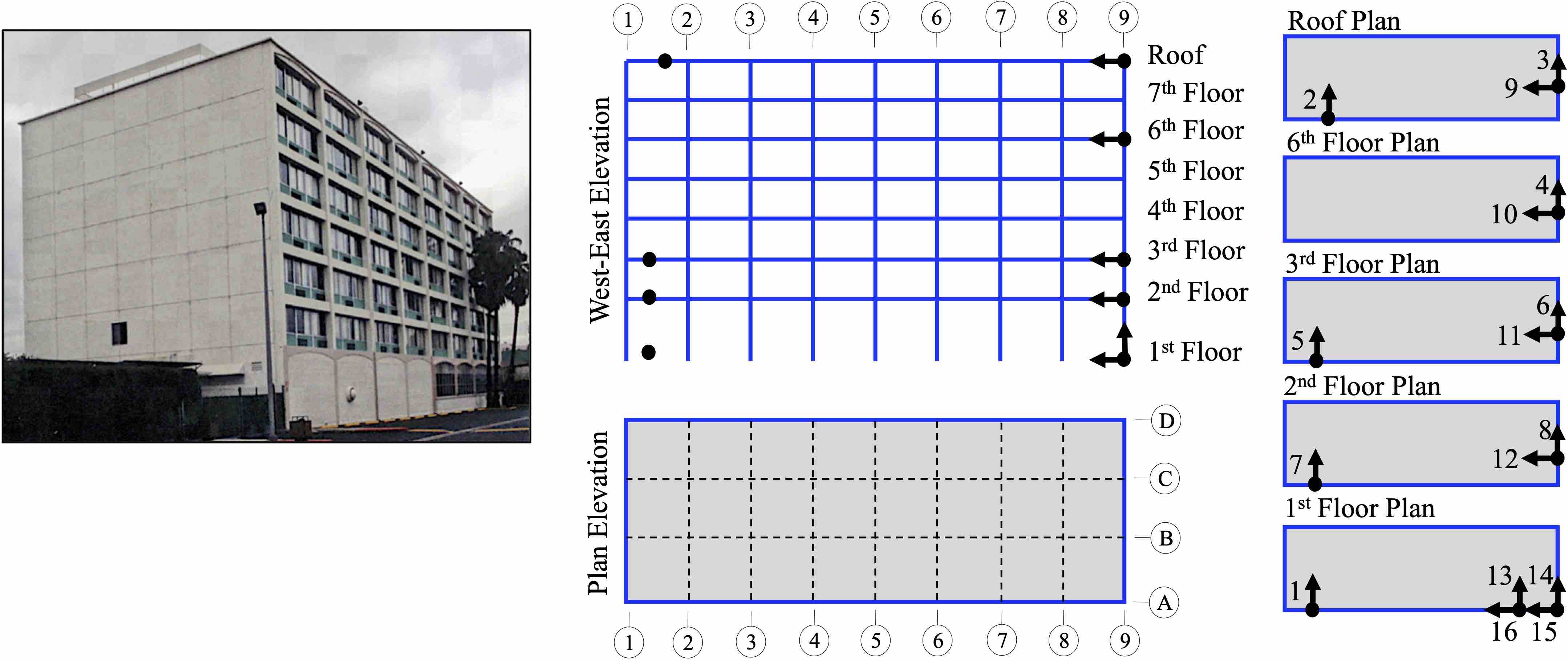
Figure 5: (left) Van Nuys hotel testbed (CSMIP Station 24386) and (Right) Location of building accelerometers on the West-East elevation and floor plans

5.3 Earthquake damage

Since the Van Nuys building was instrumented and inspected following earthquakes that affected the structure, the history of damage suffered by this building is well-documented. These documents show that the building has experienced insignificant structural and mostly nonstructural damage before the Northridge earthquake in 1994. However, the Northridge earthquake extensively damaged the building. Post-earthquake inspection red-tagged the building and revealed that the damage was severe in the south longitudinal frame (Frame A). In Frame A, five of the nine columns in the 4th story (between floors 4 and 5) were heavily damaged due to inadequate transverse reinforcement, and shear cracks ($\geq 5cm$) and bending of longitudinal reinforcement were easily visible [Trifunac and Ivanovic (2003)]. Figure 6 demonstrate the seismic damage following the 1994 Northridge earthquake in the south and north frames.

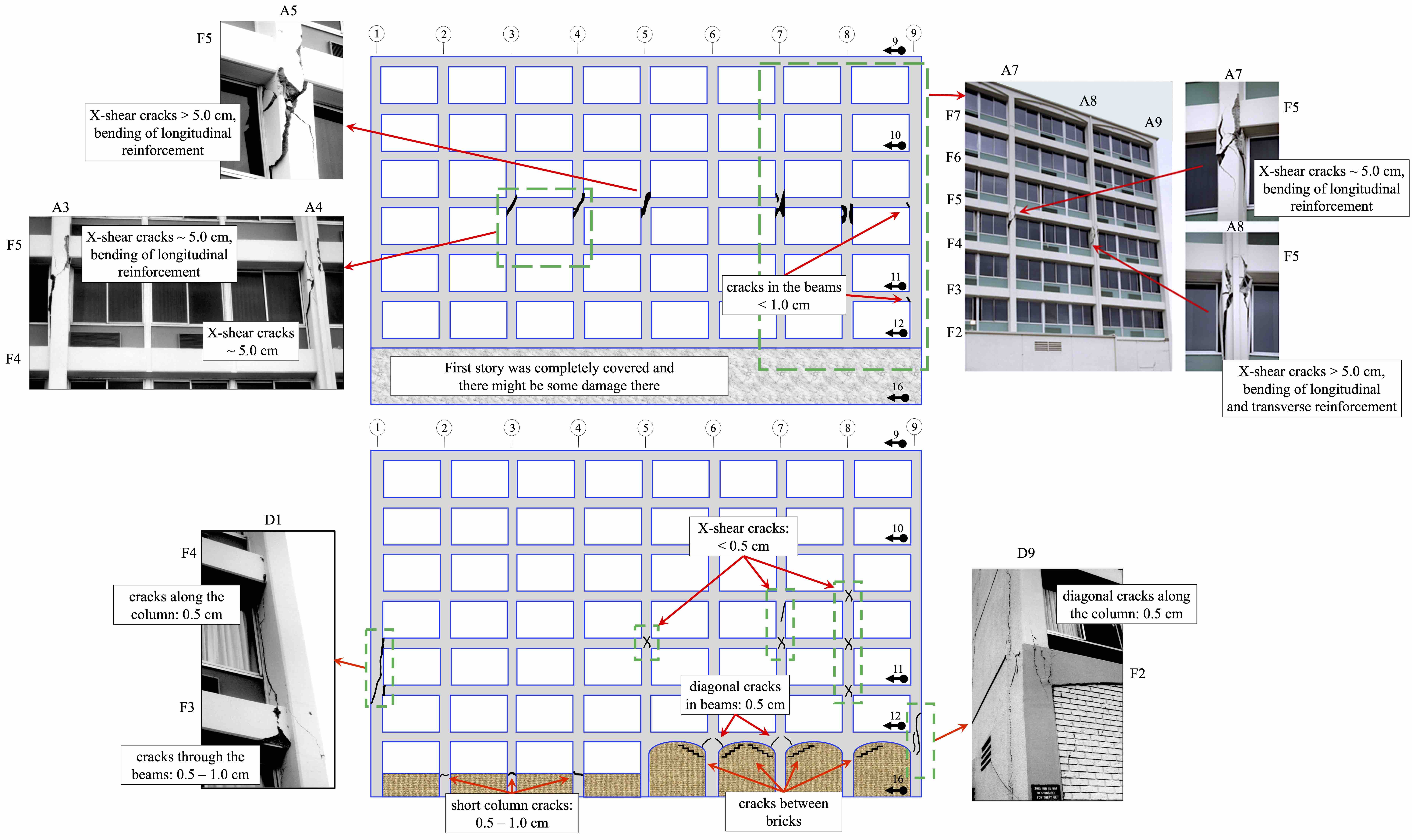
Figure 6: Schematic representation and photo records of of seismic damage following the 1994 Northridge earthquake: (top) south view of Frame A, and (bottom) south view of Frame D. (Adopted from Trifunac and Ivanovic 2003)

5.4 Previous damage assessment studies on Van Nuys building

[Browning et al. (2000)] reported the performance assessment results of the Van Nuys building based on studies of three independent research teams. These teams used nonlinear dynamic and nonlinear static analysis to localize structural damage and concluded that the various studies were successful to varying degrees. [Naeim et al. (2006)] presented a methodology for automated post-earthquake damage assessment of instrumented buildings. The methodology was applied to the measured response from Landers, Big Bear, and Northridge earthquakes. Their findings show that the building did not suffer structural damage under the Landers and Big Bear earthquakes and indicate a high probability of extensive damage to the middle floors of the building under the Northridge earthquake. They concluded that their methodology was not able to identify the exact floor level at which the damage occurs because no sensors were installed on the floor that was damaged. As previously mentioned; [Ching et al. (2006)] performed state estimation using measured data during the Northridge earthquake combined with a time-varying linear model and then, with a simplified time-varying nonlinear degradation model derived from a nonlinear finite-element model of the building. They found that state estimation using the nonlinear degradation model shows better performance and estimates the maximum ISD to be at the 4th story. They concluded that an appropriate estimation algorithm and a suitable identification model can improve the accuracy of the state estimation. [Todorovska and Trifunac (2008)] used impulse response functions computed from the recorded seismic response during 11 earthquakes, including the Northridge earthquake. They analyzed travel times of vertically propagating waves to obtain the degree and spatial distribution of changes in stiffness and infer the presence of structural damage. Their findings showed that during the Northridge earthquake, the rigidity decreased by about 60% between the ground and 2nd stories; by about 33% between 2nd and 3rd stories, and between 3rd and 6th stories; and by about 41% between the 6th story and roof. [Rodríguez et al. (2010)] implemented their proposed method called Baseline Stiffness Method to detect and assess structural and nonstructural damage to the Van Nuys building using data from the Northridge earthquake. Their approach was able to detect damage in connections with wide cracks of 5 cm or greater. On the other hand, the method identified damage in some elements of upper stories that were not detected by visual inspection reports, and also, they could not identify some of the moderate damages with small cracks. [Shan et al. (2016)] presented a model-reference damage detection algorithm of hysteretic buildings and investigated the Van Nuys hotel using measured data from Big Bear and Northridge earthquakes. The researchers concluded that their algorithm can only detect damages of certain floors and cannot detect damages in structural components or connections of the instrumented structure.

6 Implementation of the Proposed Seismic Monitoring Framework

6.1 Nonlinear modeling of the Van Nuys hotel testbed in OpenSEES

The nonlinear FE model of the building was implemented using a two-dimensional fixed-base model within the environment of OpenSEES [McKenna et al. (2000)]. This model corresponds to one of the longitudinal frames of the building (Frame A in Figure 5). In the FE model, beams and columns were modeled based on distributed plasticity modeling approach, and the force-based beam-column elements were used to accurately determine yielding and plastic deformations at the integration points along the element. Gauss-Lobatto integration approach was employed to evaluate the nonlinear response of force-based elements. Each beam and column element was discretized with four integration points, and the cross-section of each element was subdivided into fibers. The uniaxial Concrete01 material was selected to construct a Kent-Scott-Park object with a degraded linear unloading and reloading stiffness and zero tensile strength. The uniaxial Steel01 material was used to model longitudinal reinforcing steel as a bilinear model with kinematic hardening. The elasticity modulus and strain hardening parameters were assumed to be 200 GPa and 0.01, respectively. Due to insufficient transverse reinforcement in beams and columns [Jalayer et al. (2017)], an unconfined concrete model was defined to model concrete. The peak and post-peak strengths were defined at a strain of 0.002 and a compressive strain of 0.006, respectively. The corresponding strength at ultimate strain was defined as $0.05f^{\prime}_{c}$ for $f^{\prime}_{c}=34.5$ MPa and $f^{\prime}_{c}=27.6$ MPa and $0.2f^{\prime}_{c}$ for $f^{\prime}_{c}=20.7$ MPa. Based on the recommendation of [Islam (1996)], the expected yield strength of Grade 40 and Grade 60 steel were defined as 345 MPa (50 ksi) and 496 MPa (72 ksi), respectively, to account for inherent overstrength in the original material and strength gained over time.

6.2 Formulation of the OpenSEES-NMBO of Van Nuys building

The nonlinear FE model and response measurements of the Van Nuys building was employed to implement the NMBO in OpenSEES. The following subsections present the step-by-step formulation of the OpenSEES-NMBO.

6.2.1 PSD selection and numerical optimization

The PSD of ground motion, $\boldsymbol{\Phi}_{ww}(\omega)$, was characterized using the Kanai-Tajimi PSD given by

$$S(\omega)=G_{0}\frac{1+4\xi_{g}^{2}(\frac{\omega}{\omega_{g}})^{2}}{\left[1-(\frac{\omega}{\omega_{g}})^{2}\right]^{2}+4\xi_{g}^{2}(\frac{\omega}{\omega_{g}})^{2}}$$ (20)

and the amplitude modulating function $I(t)$ was selected as

$$I(t)=te^{-\alpha{t}}$$ (21)

The parameter were defined as $\xi_{g}=0.35$ for both earthquakes, $\omega_{g}=6\pi rad/s$ for Northridge earthquake and $\omega_{g}=2\pi rad/s$ for Big Bear earthquake. The underlying white noise spectral density $G_{0}$ for each direction of measured ground motion for each shake table test was found such that about 95% of the Fourier transform of the measured ground motion lies within two standard deviations of the average from the Fourier transforms of an ensemble of 200 realizations of the Kanai-Tajimi stochastic process. $\alpha$ was selected as 0.12. Details can be found in [Roohi et al. (2019a)]. Also, the PSD of measurement noise, $\boldsymbol{\Phi}_{vv}(\omega)$, in each measured channel was taken as zero mean white Gaussian sequences with a noise-to-signal root-mean-square (RMS) ratio of 0.02.

Numerical optimization was performed using Equation 14. Table 1 presents the optimized damper values for each seismic event.

Table 1: Optimized damper values in kN.s/m (kips.s/in) units

Earthquake	Story 1	Story 2	Story 5	Story 7
Big Bear	7283.11 (41.59)	9357.25 (53.43)	19299.40 (110.20)	34808.04 (198.76)
Northridge	5209.72 (29.75)	6592.45 (37.64)	16612.79 (94.86)	47217.69 (269.62)

6.2.2 Formulation of the OpenSEES-NMBO

The OpenSEES nonlinear FE model was modified by adding grounded dampers in measurement locations and was subjected to corrective forces. Dynamic analysis was performed to estimate the complete seismic response. Figure 7 presents a schematic of the Van Nuys hotel testbed (with the location of accelerometers) along with the OpenSEES-NMBO (with corresponding added viscous dampers and corrective forces in measurement locations).

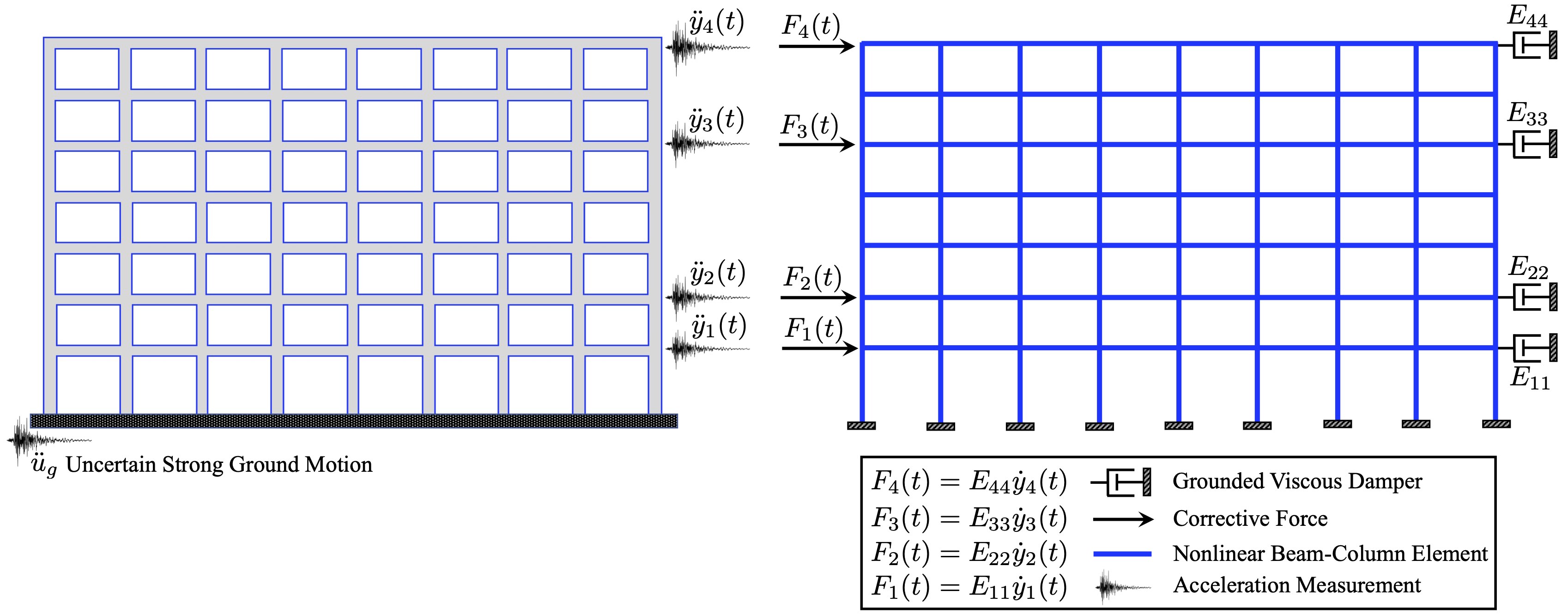
Figure 7: Schematic of the Van Nuys hotel testbed with location of accelerometers (left) and the OpenSEES-NMBO with corresponding added viscous dampers and corrective forces in measurement locations

6.3 Seismic damage reconstruction using estimated seismic response

Once the complete seismic response is estimated using the OpenSEES-NMBO, the seismic damage to the building can be quantified according to the Section 4.0.3. This subsection demonstrates the procedure in more detail.

6.3.1 Shear DCR reconstruction

The shear DCRs were estimated based on the Equation 18. The shear demands were obtained from OpenSEES-NMBO, and the capacity of columns were calculated based on the Section 6.5.2.3.1 of [FEMA (2000)].

6.3.2 Ductility demand reconstruction

The seismic damage caused by excessive deformation is the first term of the Equation 19 given by:

$$DI_{\mu}=\dfrac{\mu_{m}}{\mu_{u}}$$ (22)

where, the $\mu_{m}$ in each structural element is expressed by the maximum estimated curvature along integration points normalized by the yield curvature given by

$$\mu_{m}=max\{{\dfrac{\phi_{m,j}}{\phi_{y}}}\}_{j=1:N_{p}}$$ (23)

here, $\phi_{m,j}$ is maximum estimated curvature in integration point $j$, $\phi_{y}$ is curvature capacity and $N_{p}$ is number of integration points along element. The curvature ductility capacity ($\mu_{u}$) is obtained by

$$\begin{aligned} &\mu_{u}=\dfrac{\phi_{u}}{\phi_{y}}\end{aligned}$$ (24)

where $\phi_{u}$ is the ultimate curvature capacity of the section.

6.3.3 Dissipated hysteretic energy reconstruction

The seismic damage caused by dissipated hysteretic energy, $DI_{E}$ in Equation 19, was calculated based on flexure failure mode as follows

$$DI_{E}=\psi\dfrac{E_{h}}{E_{max}}\cong\psi\dfrac{E_{h}}{M_{y}\theta_{y}\mu_{u}}$$ (25)

where $M_{y}$ is yield moment and $\theta_{y}$ is yield rotation angle. The main issue with the calculation of $DI_{E}$ is the determination of $\psi$, which usually is calibrated to a number between 0.05 or 0.15. A reasonable $\psi$ value should properly account for the effect of load cycles causing structural damage. The selection of small value for $\psi$ neglects the effect of the $DI_{E}$ in the overall damage index [Williams and Sexsmith (1995)]. Since the true $\psi$ is unknown for the elements of Van Nuys building and in the scope of this paper, the objective is to localize seismic damage, the calibration parameter is set to one, and the estimated value of each term in the damage index will be first reported separately and then combined.

The dissipated hysteretic energy ($E_{h}$) is estimated based on Equation 7 and the seismic response estimated using OpenSEES-NMBO. The parameter $M_{y}$ was obtained based on section analysis and the value of $\theta_{y}\mu_{u}$ calculated as follows

$$\theta_{y}\mu_{u}=\theta_{p}=(\phi_{u}-\phi_{y})l_{p}=\phi_{p}l_{p}$$ (26)

where $l_{p}$ is the plastic hinge length and is defined using an empirically validated relationship proposed by [Bae and Bayrak (2008)] given by

$$\dfrac{l_{p}}{h}=\left[0.3\left(\dfrac{P}{P_{o}}\right)+\left(\dfrac{A_{s}}{A_{g}}\right)-1\right]\left(\dfrac{L}{h}\right)+0.25\geq 0.25$$ (27)

where $h$ and $L$ represent depth and length of column; $A_{g}$ and $A_{s}$ denote gross area of concrete section and area of tension reinforcement; $f^{\prime}_{c}$ and $f_{y}$ are compressive strength of concrete and yield stress of reinforcement; and $P_{o}=0.85f^{\prime}_{c}(A_{g}-A_{s})+f_{y}A_{s}$.

7 Seismic Response and Damage Reconstruction Results

A summary of the seismic response and damage reconstruction results is presented in this section to validate the proposed seismic monitoring framework.

7.1 Displacement estimation results

First, we compare the displacement estimates using OpenSEES-NMBO and its uncertainty with those obtained from 1) response measurements and 2) open-loop analysis under measured ground motion at instrumented and non-instrumented stories. Figures 8 and 9 present the comparison of the displacement estimates at instrumented 1st and 7th stories and non-instrumented 3rd and 6th stories during the Big Bear earthquake and Northridge earthquake, respectively.

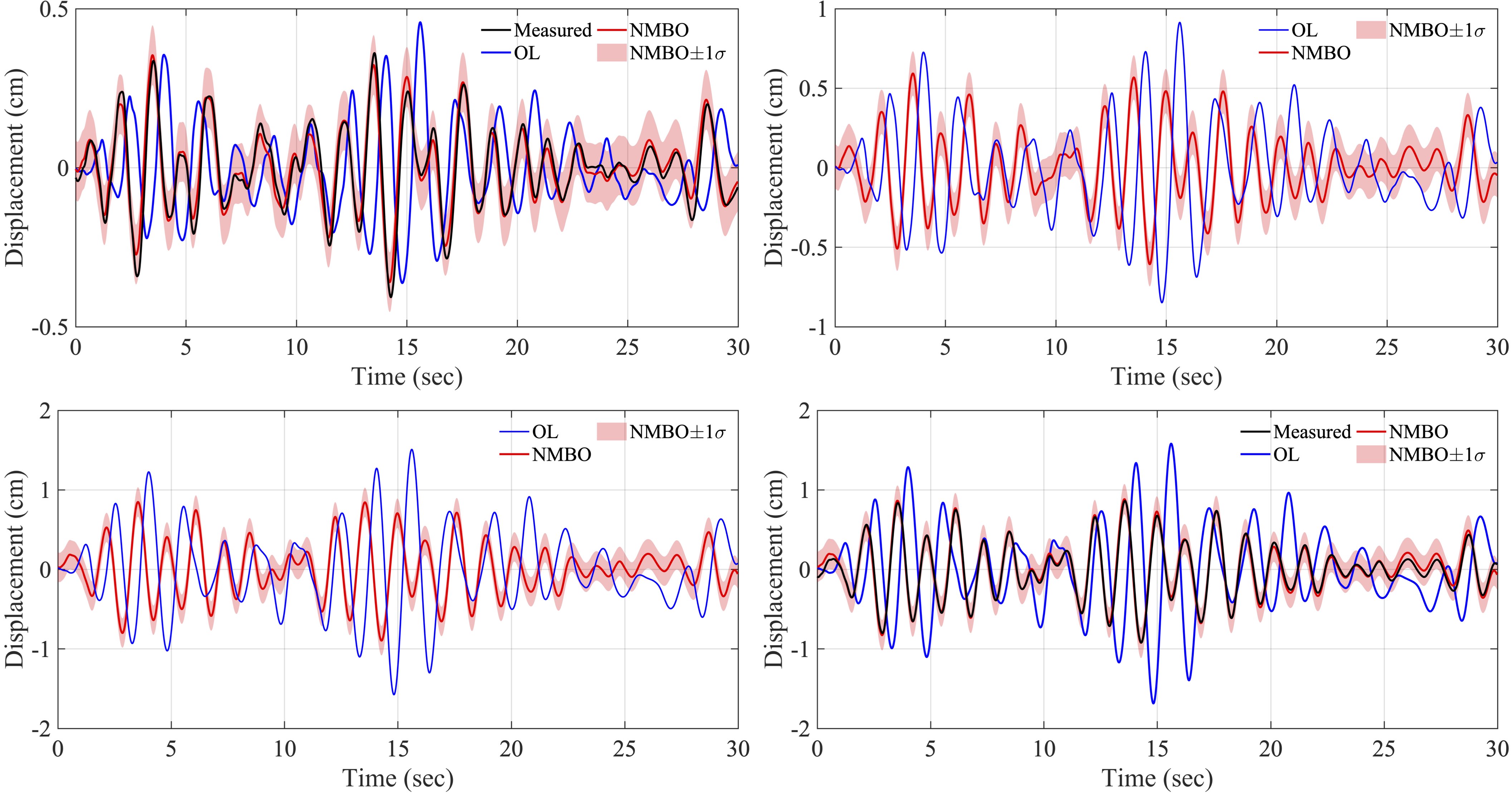
Figure 8: Comparison of displacement estimates using OpenSEES-NMBO with estimates using open-loop analysis and actual measurements in 1st floor (top left), 3rd floor (top right), 6th floor (bottom left) and 7th floor (bottom right) during Big Bear earthquake. The Measured represents measured response, the OL represents the open-loop analysis of OpenSEES model under measured ground motion and the NMBO represents the estimated response using the OpenSEES-NMBO with sensor measurements from measured location along with $1\sigma$ estimation uncertainty bound

7.2 Inter-story drift estimation results

Figure 10 depicts the estimated $\text{ISD}_{\mathrm{max}}$ ratios and their corresponding $1\sigma$ confidence intervals using OpenSEES-NMBO. These results are compared with estimated $\text{ISD}_{\mathrm{max}}$ using open-loop analysis and those obtained from instrumented stories. The OpenSEES-NMBO ISD estimates indicate that the building could be classified as IO following the Big Bear earthquake and as LS-CP following the Northridge earthquake. The actual performance and post-earthquake inspection reports of the buildings validate the accuracy of the performance estimates. Figure 11 gives an in-depth examination of the ISD estimates during the Northridge earthquake. The left plot in this figure shows the comparison of ISDs at 3rd, 4th, and 5th stories, and the right plot shows the comparison of relative ISDs between floors 3 and 4 and also, floors 4 and 5. Here, the relative ISD is defined as follows

$$\text{RISD}_{(k,k-1)}=\text{ISD}_{(k)}-\text{ISD}_{(k-1)}$$ (28)

where $\text{RISD}_{(k,k-1)}$ is relative ISD between stories $k$ and $k-1$. The estimation results show that even though the $\text{ISD}_{\mathrm{max}}$ occurs in the third story, the RISD demand between floors 4 and 5 is higher than floors 3 and 4.

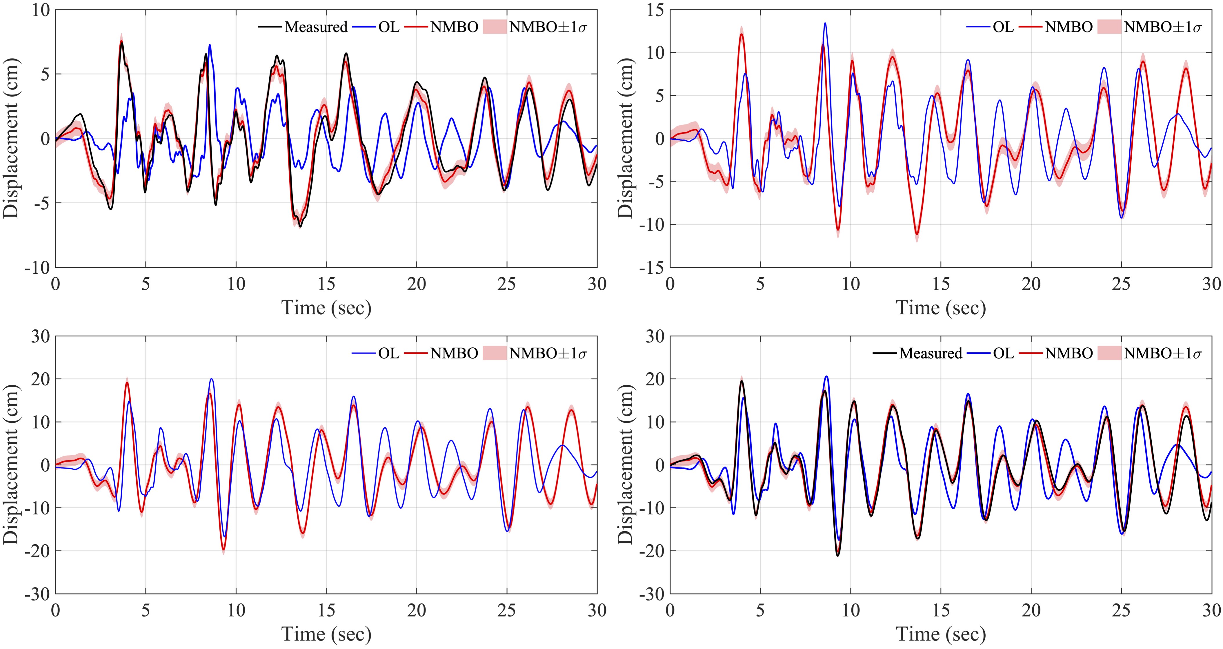
Figure 9: Comparison of displacement time history estimates with estimates using open-loop analysis and actual measurements in 1st floor (top left), 3rd floor (top right), 6th floor (bottom left) and 7th floor (bottom right) during Northridge earthquake.

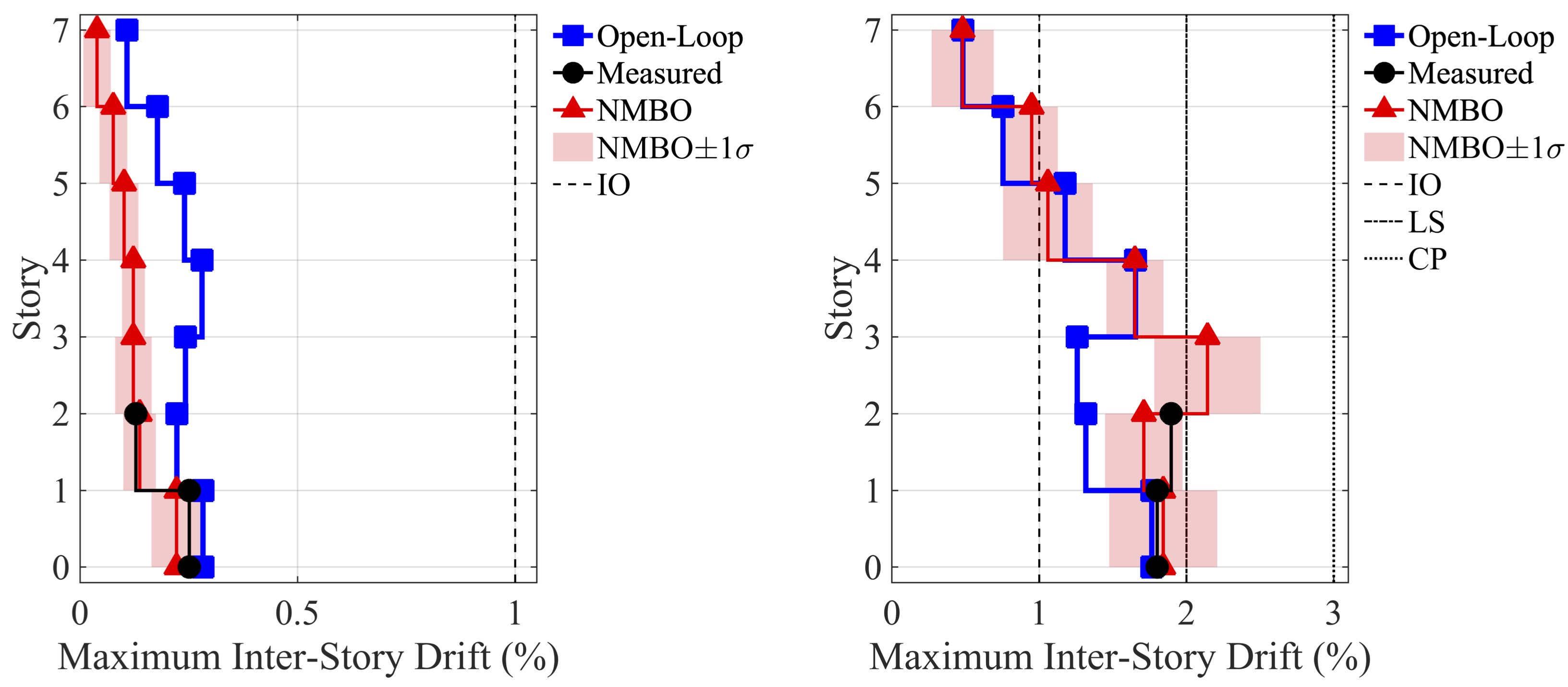
Figure 10: Comparison of $\text{ISD}_{\mathrm{max}}$ ratios obtained from response measurements with those estimated using OpenSEES-NMBO and open-loop analysis during 1992 Big Bear earthquake (left) and 1994 Northridge earthquake (right).

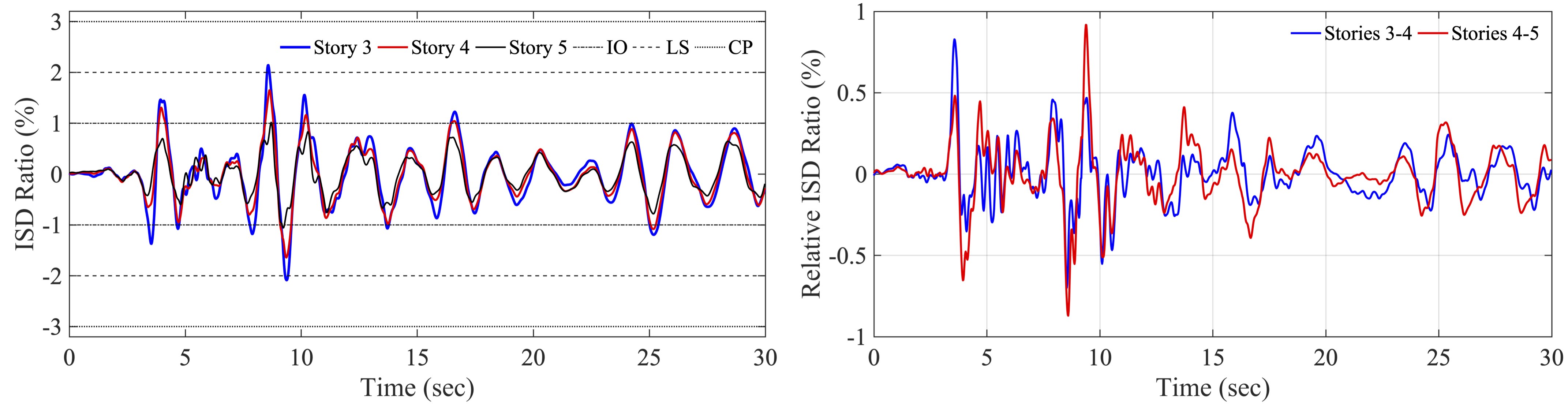
Figure 11: Comparison of ISD (left) and RISD (right) time history estimates for stories 3 to 5 during Northridge earthquake.

7.3 Elemet-by-element shear demand to capacity ratio reconstruction

Figure 12 shows results for shear estimated element-by-element shear DCR ratios by OpenSEES-NMBO using measured seismic response of the Van Nuys building during Big Bear (left) and Northridge (right) earthquakes.

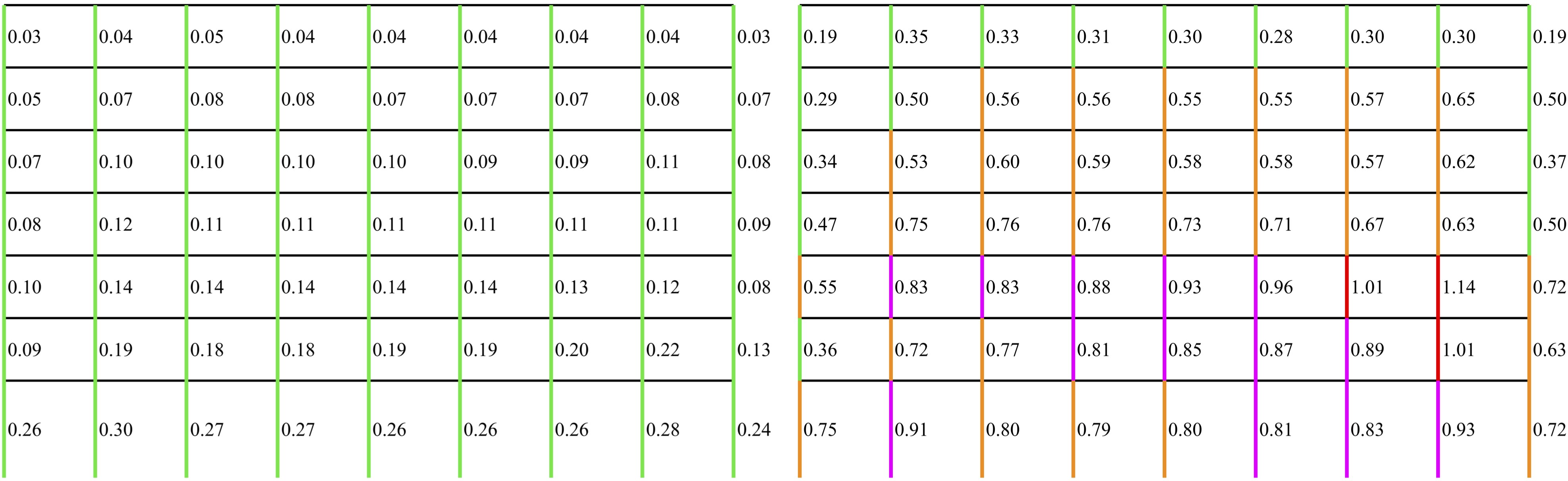
Figure 12: Estimated element-by-element shear demand to capacity ratios by OpenSEES-NMBO using measured seismic response of the Van Nuys building during 1992 Big Bear (left) and 1994 Northridge (right) earthquakes.

7.4 Element-by-element damage index reconstruction

This section presents the seismic damage quantification results using the estimated response from OpenSEES-NMBO and the damage model presented at Section 4.0.3, which is also demonstrated in more detail in Section 6.3. Figure 13 summarizes the estimated maximum curvature ductility demands ($\mu_{m}$) in two ends of columns for each earthquake. To interpret the $\mu_{m}$ demands, one needs to consider that the expected ductility capacity of columns in this building is relatively low as the columns are non-ductile. Figure 14 presents reconstructed element-by-element normalized energy dissipation. Figure 15 presents the reconstructed element-by-element damage indices. Figure 16 schematically depicts the seismic damage suffered during the Northridge earthquake to compare the reconstructed DIs with the building’s actual performance. The shear cracks with $\text{width}\geq 5cm$ are highlights in red color and the shear cracks ($0.5cm\leq\text{width}\leq 1$) are highlights in green color. As can be seen, the element-by-element comparison of estimated DIs with post-earthquake inspection results confirms the accuracy of damage localization using the proposed mechanistic approach.

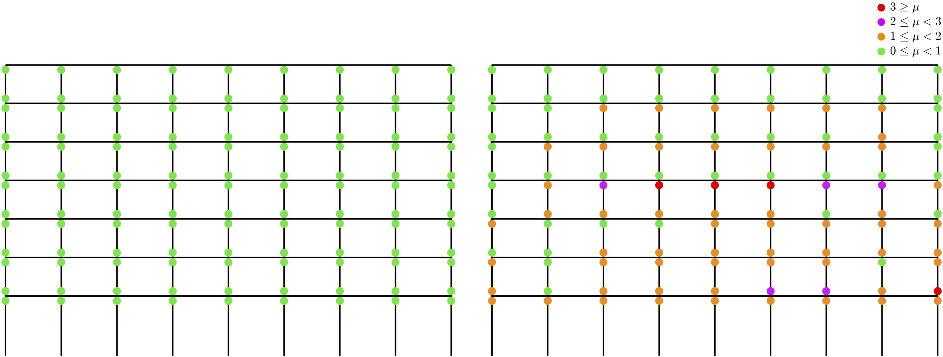
Figure 13: Reconstructed maximum end curvature ductility demands in columns by implementing OpenSEES-NMBO using measured seismic response of the Van Nuys building during 1992 Big Bear (left) and 1994 Northridge (right) earthquakes.

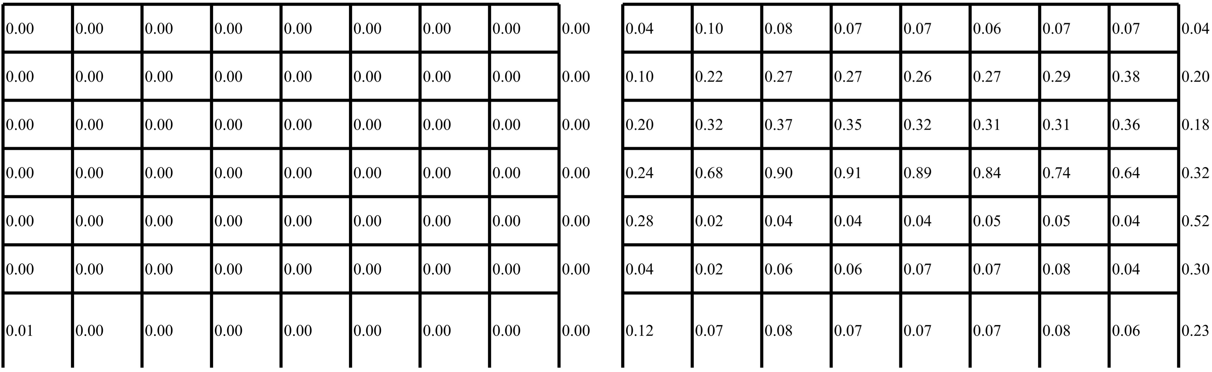
Figure 14: Reconstructed element-by-element normalized energy dissipation by OpenSEES-NMBO using measured seismic response of the Van Nuys building during 1992 Big Bear (left) and 1994 Northridge (right) earthquakes.

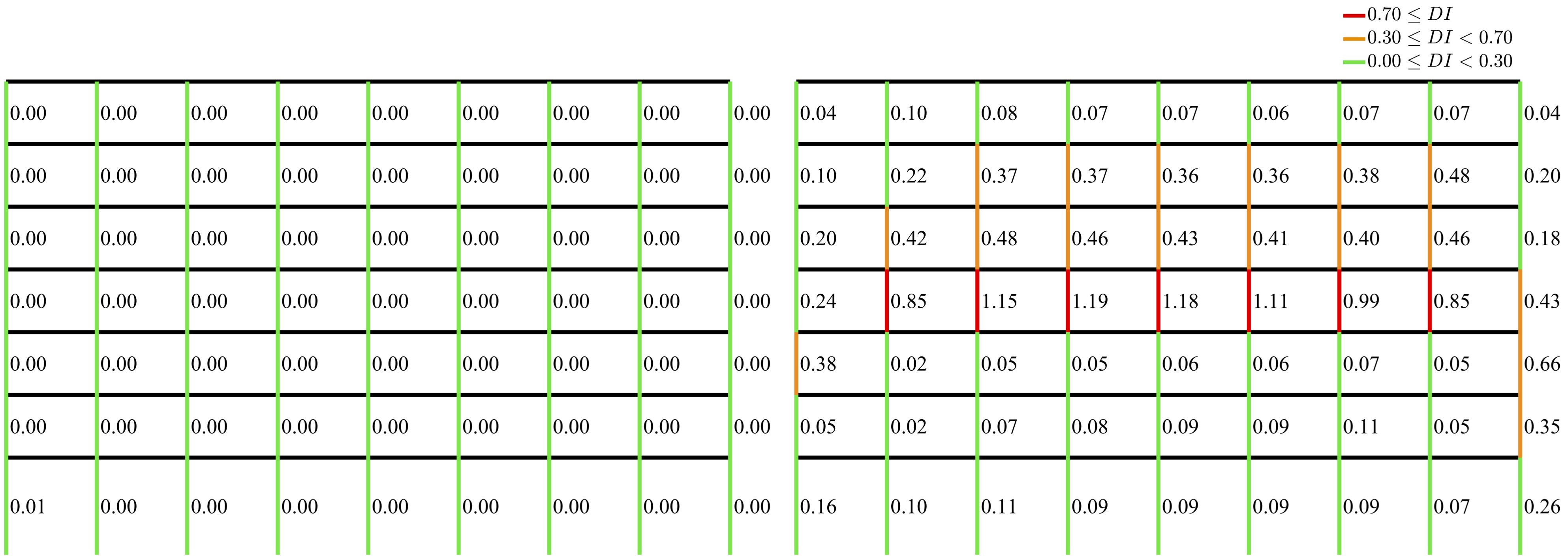
Figure 15: Reconstructed element-by-element damage indices by OpenSEES-NMBO using measured seismic response of the Van Nuys building during 1992 Big Bear (left) and 1994 Northridge (right) earthquakes.

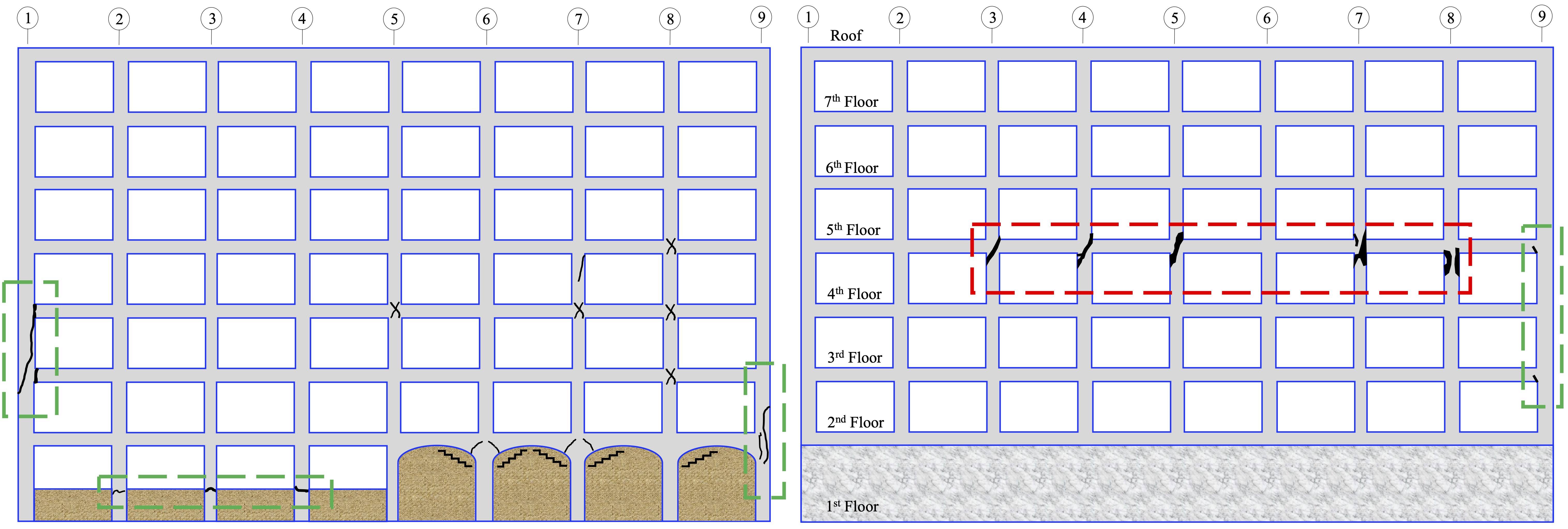
Figure 16: Seismic damage experienced during the 1994 Northridge earthquake: (left) south view of Frame D, and (right) south view of Frame A. (Adopted from Trifunac and Ivanovic 2003)

7.5 Discussion on damage detection and localization results

The results described in the preceding sections demonstrate that a nonlinear model-data fusion using a refined distributed plasticity FE model and a limited number of response measurements can accurately reconstruct the seismic response. Subsequently, the estimated response can be used to quantify the seismic damage based on damage sensitive response parameters and damage models. The estimated ISDs indicated that the performance-based post-earthquake re-occupancy category of the building was IO during the Big Bear earthquake and LS-CP during the Northridge earthquake. The ISD and RISD analysis during the Northridge earthquake showed that the $\text{ISD}_{\mathrm{max}}$ occurred at the 3rd story, while the maximum RISD occurs at the top of the 4th story. Also, dissipated energy and ductility reconstruction detects no structural damage during the Big Bear earthquake and severe damage during the Northridge earthquake. By combining the information from estimated ISDs, RISDs, maximum curvature ductility demands, and element-by-element damage indices during the Northridge earthquake, severe damage was localized in the columns of the 4th story (between floors 4 and 5) and also, small or moderate damage was estimated for the remaining columns. The location of severe damage in the 4th story can be explained mainly by widely spaced or absent transverse reinforcing in the beam-column joints contributed to the lower shear capacity of the story; which can be accounted for by the proposed mechanistic seismic monitoring framework through high-resolution seismic response and element-by-element damage index reconstruction. Finally, it was shown that the damage assessment results were consistent with the building’s actual performance and post-earthquake inspection reports following the Big Bear and Northridge earthquakes. Therefore, the applicability of the proposed framework is validated in the context of a real-world building that experienced severe localized damage during sequential seismic events.

8 Conclusions

This paper proposes a seismic monitoring framework to reconstruct element-by-element dissipated hysteretic energy and perform structural damage detection and localization. The framework employs a nonlinear model-based state observer (NMBO) to combine a design level nonlinear FE model with acceleration measurements at limited stories to estimate nonlinear seismic response at all DoF of the model. The estimated response is then used to reconstruct damage-sensitive response features, including 1) inter-story drifts, 2) code-based demand to capacity ratios, and 3) normalized dissipated hysteretic energy and ductility demands. Ultimately, the estimated features are used to conduct the performance-based post-earthquake assessment, damage detection, and localization.

The methodology was successfully validated using measured data from the seven-story Van Nuys hotel testbed instrumented by CSMIP (Station 24386) during 1992 Big Bear and 1994 Northridge earthquakes. The NMBO of the building was implemented using a distributed plasticity finite element model and measured data to reconstruct seismic response during each earthquake. The estimated seismic response was then used to reconstruct inter-story drifts and determine the performance-based post-earthquake re-occupation category of the building following each earthquake. The performance categories were estimated as IO and LS-CP during the Big Bear and Northridge earthquakes, respectively. Analysis during the Northridge earthquake showed that the maximum inter-story drift occurred at the 3rd story, while the maximum relative inter-story drift occurred at the top of the 4th story. Column-by-column shear demand to capacity ratios, ductility demands, and normalized dissipated hysteretic energy ratios were computed. The proposed framework correctly estimated linear behavior and no damage during the Big Bear earthquake and identified the location of major damage in the beam/column joints located at the fourth floor of the south frame during the Northridge earthquake. The damage indices were identified near unity and above (which corresponds to total failure of the member) in columns with severe damages (wide shear cracks equal or greater than 5 $cm$); between 0.35 and 0.70 in columns with moderate damage (shear cracks smaller than 1 $cm$); and smaller than 0.50 in the remaining columns which did not experienced visible cracks. To the best knowledge of authors, the results presented in this paper constitute the most accurate and the highest resolution damage estimates obtained for the Van Nuys hotel testbed.

9 Data Availability Statement

Some or all data, models, or code that support the findings of this study are available from the corresponding author upon reasonable request.

10 Acknowledgement

Support for this research provided, in part, by award No. 1453502 from the National Science Foundation is gratefully acknowledged.

References

- Bae and Bayrak (2008) Bae, S. and Bayrak, O. (2008). “Plastic hinge length of reinforced concrete columns.” ACI Structural Journal, 105(3), 290.
- Bernal and Hernandez (2006) Bernal, D. and Hernandez, E. (2006). “A data-driven methodology for assessing impact of earthquakes on the health of building structural systems.” The Structural Design of Tall and Special Buildings, 15(1), 21–34.
- Browning et al. (2000) Browning, J., Li, Y. R., Lynn, A., and Moehle, J. P. (2000). “Performance assessment for a reinforced concrete frame building.” Earthquake Spectra, 16(3), 541–556.
- Ching et al. (2006) Ching, J., Beck, J. L., Porter, K. A., and Shaikhutdinov, R. (2006). “Bayesian state estimation method for nonlinear systems and its application to recorded seismic response.” Journal of Engineering Mechanics, 132(4), 396–410.
- Doucet et al. (2000) Doucet, A., Godsill, S., and Andrieu, C. (2000). “On sequential monte carlo sampling methods for bayesian filtering.” Statistics and computing, 10(3), 197–208.
- FEMA (2000) FEMA (2000). “Prestandard and commentary for the seismic rehabilitation of buildings.” American Society of Civil Engineers (ASCE).
- Frizzarin et al. (2010) Frizzarin, M., Feng, M. Q., Franchetti, P., Soyoz, S., and Modena, C. (2010). “Damage detection based on damping analysis of ambient vibration data.” Structural Control and Health Monitoring, 17(4), 368–385.
- Gelb (1974) Gelb, A. (1974). Applied optimal estimation. MIT press.
- Gičev and Trifunac (2012) Gičev, V. and Trifunac, M. D. (2012). “A note on predetermined earthquake damage scenarios for structural health monitoring.” Structural control and health monitoring, 19(8), 746–757.
- Goel (2005) Goel, R. K. (2005). “Evaluation of modal and fema pushover procedures using strong-motion records of buildings.” Earthquake spectra, 21(3), 653–684.
- Hernandez et al. (2018) Hernandez, E., Roohi, M., and Rosowsky, D. (2018). “Estimation of element-by-element demand-to-capacity ratios in instrumented smrf buildings using measured seismic response.” Earthquake Engineering & Structural Dynamics, 47(12), 2561–2578.
- Hernandez (2011) Hernandez, E. M. (2011). “A natural observer for optimal state estimation in second order linear structural systems.” Mechanical Systems and Signal Processing, 25(8), 2938–2947.
- Hernandez (2013) Hernandez, E. M. (2013). “Optimal model-based state estimation in mechanical and structural systems.” Structural control and health monitoring, 20(4), 532–543.
- Hernandez and May (2012) Hernandez, E. M. and May, G. (2012). “Dissipated energy ratio as a feature for earthquake-induced damage detection of instrumented structures.” Journal of Engineering Mechanics, 139(11), 1521–1529.
- Islam (1996) Islam, M. S. (1996). “Analysis of the northridge earthquake response of a damaged non-ductile concrete frame building.” The structural design of tall buildings, 5(3), 151–182.
- Jalayer et al. (2017) Jalayer, F., Ebrahimian, H., Miano, A., Manfredi, G., and Sezen, H. (2017). “Analytical fragility assessment using unscaled ground motion records.” Earthquake Engineering & Structural Dynamics, 46(15), 2639–2663.
- Krawinkler (2005) Krawinkler, H. (2005). Van Nuys hotel building testbed report: exercising seismic performance assessment. Pacific Earthquake Engineering Research Center, College of Engineering ….
- Krawinkler and Zohrei (1983) Krawinkler, H. and Zohrei, M. (1983). “Cumulative damage in steel structures subjected to earthquake ground motions.” Computers & Structures, 16(1-4), 531–541.
- Li and Jirsa (1998) Li, Y. R. and Jirsa, J. O. (1998). “Nonlinear analyses of an instrumented structure damaged in the 1994 northridge earthquake.” Earthquake Spectra, 14(2), 265–283.
- Loh and LIN (1996) Loh, C.-H. and LIN, H.-M. (1996). “Application of off-line and on-line identification techniques to building seismic response data.” Earthquake engineering & structural dynamics, 25(3), 269–290.
- McKenna et al. (2000) McKenna, F., Fenves, G. L., Scott, M. H., et al. (2000). “Open system for earthquake engineering simulation.” University of California, Berkeley, CA.
- Naeim et al. (2006) Naeim, F., Lee, H., Hagie, S., Bhatia, H., Alimoradi, A., and Miranda, E. (2006). “Three-dimensional analysis, real-time visualization, and automated post-earthquake damage assessment of buildings.” The Structural Design of Tall and Special Buildings, 15(1), 105–138.
- Park and Ang (1985) Park, Y.-J. and Ang, A. H.-S. (1985). “Mechanistic seismic damage model for reinforced concrete.” Journal of structural engineering, 111(4), 722–739.
- Pioldi et al. (2017) Pioldi, F., Ferrari, R., and Rizzi, E. (2017). “Seismic fdd modal identification and monitoring of building properties from real strong-motion structural response signals.” Structural Control and Health Monitoring, 24(11), e1982.
- Rodríguez et al. (2010) Rodríguez, R., Escobar, J. A., and Gómez, R. (2010). “Damage detection in instrumented structures without baseline modal parameters.” Engineering Structures, 32(6), 1715–1722.
- Roohi (2019a) Roohi, Milad, H.-E. R. D. (September 10-12, 2019a). “Nonlinear seismic response reconstruction in minimally instrumented buildings— validation using neeswood capstone full-scale tests.” 2519–2526.
- Roohi (2019b) Roohi, M. (2019b). “Performance-based seismic monitoring of instrumented buildings.” Ph.D. thesis, Graduate College Dissertations and Theses. 1140. University of Vermont., Graduate College Dissertations and Theses. 1140. University of Vermont.
- Roohi et al. (2019a) Roohi, M., Hernandez, E. M., and Rosowsky, D. (2019a). “Nonlinear seismic response reconstruction and performance assessment in minimally instrumented wood-frame buildings - validation using neeswood capstone full-scale tests.” Structural Control & Health Monitoring, e2373.
- Roohi et al. (2019b) Roohi, M., Hernandez, E. M., and Rosowsky, D. (2019b). “Seismic damage assessment of instrumented wood-frame buildings: A case-study of neeswood full-scale shake table tests.” arXiv preprint arXiv:1902.09955.
- Shan et al. (2016) Shan, J., Shi, W., and Lu, X. (2016). “Model-reference health monitoring of hysteretic building structure using acceleration measurement with test validation.” Computer-Aided Civil and Infrastructure Engineering, 31(6), 449–464.
- Stephens and Yao (1987) Stephens, J. E. and Yao, J. T. (1987). “Damage assessment using response measurements.” Journal of Structural Engineering, 113(4), 787–801.
- Sucuoglu and Erberik (2004) Sucuoglu, H. and Erberik, A. (2004). “Energy-based hysteresis and damage models for deteriorating systems.” Earthquake engineering & structural dynamics, 33(1), 69–88.
- Taghavi and Miranda (2005) Taghavi, S. and Miranda, E. (2005). “Approximate floor acceleration demands in multistory buildings. ii: Applications.” Journal of Structural Engineering, 131(2), 212–220.
- Taucer et al. (1991) Taucer, F., Spacone, E., and Filippou, F. C. (1991). A fiber beam-column element for seismic response analysis of reinforced concrete structures, Vol. 91. Earthquake Engineering Research Center, College of Engineering, University ….
- Teran-Gilmore and Jirsa (2007) Teran-Gilmore, A. and Jirsa, J. O. (2007). “Energy demands for seismic design against low-cycle fatigue.” Earthquake engineering & structural dynamics, 36(3), 383–404.
- Todorovska and Trifunac (2008) Todorovska, M. I. and Trifunac, M. D. (2008). “Impulse response analysis of the van nuys 7-storey hotel during 11 earthquakes and earthquake damage detection.” Structural Control and Health Monitoring, 15(1), 90–116.
- Trifunac and Ebrahimian (2014) Trifunac, M. and Ebrahimian, M. (2014). “Detection thresholds in structural health monitoring.” Soil Dynamics and Earthquake Engineering, 66, 319–338.
- Trifunac and Ivanovic (2003) Trifunac, M. and Ivanovic, S. (2003). “Analysis of drifts in a seven-story reinforced concrete structure.” University of Southern California Report CE, 03–10.
- Trifunac et al. (1999) Trifunac, M., Ivanovic, S., and Todorovska, M. (1999). “Instrumented 7-storey reinforced concrete building in van nuys, california: description of the damage from the 1994 northridge earthquake and strong motion data.” Report CE 99, 2.
- Uang and Bertero (1990) Uang, C.-M. and Bertero, V. V. (1990). “Evaluation of seismic energy in structures.” Earthquake Engineering & Structural Dynamics, 19(1), 77–90.
- van de Lindt et al. (2010) van de Lindt, J. W., Gupta, R., Pei, S., Tachibana, K., Araki, Y., Rammer, D., and Isoda, H. (2010). “Damage assessment of a full-scale six-story wood-frame building following triaxial shake table tests.” Journal of Performance of Constructed Facilities, 26(1), 17–25.
- Wan and Van Der Merwe (2000) Wan, E. A. and Van Der Merwe, R. (2000). “The unscented kalman filter for nonlinear estimation.” Proceedings of the IEEE 2000 Adaptive Systems for Signal Processing, Communications, and Control Symposium (Cat. No. 00EX373), Ieee, 153–158.
- Williams and Sexsmith (1995) Williams, M. S. and Sexsmith, R. G. (1995). “Seismic damage indices for concrete structures: a state-of-the-art review.” Earthquake spectra, 11(2), 319–349.