Abstract

The performance of the code a compiler generates depends on the order in which it applies the optimization passes. Choosing a good order–often referred to as the phase-ordering problem, is an NP-hard problem. As a result, existing solutions rely on a variety of heuristics. In this paper, we evaluate a new technique to address the phase-ordering problem: deep reinforcement learning. To this end, we implement AutoPhase: a framework that takes a program and uses deep reinforcement learning to find a sequence of compilation passes that minimizes its execution time. Without loss of generality, we construct this framework in the context of the LLVM compiler toolchain and target high-level synthesis programs. We use random forests to quantify the correlation between the effectiveness of a given pass and the program’s features. This helps us reduce the search space by avoiding phase orderings that are unlikely to improve the performance of a given program. We compare the performance of AutoPhase to state-of-the-art algorithms that address the phase-ordering problem. In our evaluation, we show that AutoPhase improves circuit performance by 28% when compared to using the -O3 compiler flag, and achieves competitive results compared to the state-of-the-art solutions, while requiring fewer samples. Furthermore, unlike existing state-of-the-art solutions, our deep reinforcement learning solution shows promising result in generalizing to real benchmarks and 12,874 different randomly generated programs, after training on a hundred randomly generated programs.

1 Introduction

High-Level Synthesis (HLS) automates the process of creating digital hardware circuits from algorithms written in high-level languages. Modern HLS tools Xilinx (2019); Intel (2019); Canis et al. (2013) use the same front-end as the traditional software compilers. They rely on traditional software compiler techniques to optimize the input program’s intermediate representation (IR) and produce circuits in the form of RTL code. Thus, the quality of compiler front-end optimizations directly impacts the performance of HLS-generated circuit.

Program optimization is a notoriously difficult task. A program must be just in ”the right form” for a compiler to recognize the optimization opportunities. This is a task a programmer might be able to perform easily, but is often difficult for a compiler. Despite a decade of research on developing sophisticated optimization algorithms, there is still a performance gap between the HLS generated code and the hand-optimized one produced by experts.

In this paper, we build off the LLVM compiler Lattner & Adve (2004). However, our techniques, can be broadly applicable to any compiler that uses a series of optimization passes. In this case, the optimization of an HLS program consists of applying a sequence of analysis and optimization phases, where each phase in this sequence consumes the output of the previous phase, and generates a modified version of the program for the next phase. Unfortunately, these phases are not commutative which makes the order in which these phases are applied critical to the performance of the output.

Consider the program in Figure 1, which normalizes a vector. Without any optimizations, the norm function will take $\Theta(n^{2})$ to normalize a vector. However, a smart compiler will implement the loop invariant code motion (LICM) Muchnick (1997) optimization, which allows it to move the call to mag above the loop, resulting in the code on the left column in Figure 2. This optimization brings the runtime down to $\Theta(n)$—a big speedup improvement. Another optimization the compiler could perform is (function) inlining Muchnick (1997). With inlining, a call to a function is simply replaced with the body of the function, reducing the overhead of the function call. Applying inlining to the code will result in the code in the right column of Figure 2.

⬇

__attribute__((const))

double mag(int n, const double *A) {

double sum = 0;

for(int i=0; i<n; i++){

sum += A[i] * A[i];

}

return sqrt(sum);

}

void norm(int n, double *restrict out,

const double *restrict in) {

for(int i=0; i<n; i++) {

out[i] = in[i] / mag(n, in);

}

}

Figure 1: A simple program to normalize a vector.

⬇

void norm(int n, double *restrict out,

const double *restrict in) {

double precompute = mag(n, in);

for(int i=0; i<n; i++) {

out[i] = in[i] / precompute;

}

}

⬇

void norm(int n, double *restrict out,

const double *restrict in) {

double precompute, sum = 0;

for(int i=0; i<n; i++){

sum += A[i] * A[i];

}

precompute = sqrt(sum);

for(int i=0; i<n; i++) {

out[i] = in[i] / precompute;

}

}

Figure 2: Progressively applying LICM (left) then inlining (right) to the code in Figure 1.

⬇

void norm(int n, double *restrict out,

const double *restrict in) {

for(int i=0; i<n; i++) {

double sum = 0;

for(int j=0; j<n; j++){

sum += A[j] * A[j];

}

out[i] = in[i] / sqrt(sum);

}

}

⬇

void norm(int n, double *restrict out,

const double *restrict in) {

double sum;

for(int i=0; i<n; i++) {

sum = 0;

for(int j=0; j<n; j++){

sum += A[j] * A[j];

}

out[i] = in[i] / sqrt(sum);

}

}

Figure 3: Progressively applying inlining (left) then LICM (right) to the code in Figure 1.

Now, consider applying these optimization passes in the opposite order: first inlining then LICM. After inlining, we get the code on the left of Figure 3. Once again we get a modest speedup, having eliminated $n$ function calls, though our runtime is still $\Theta(n^{2})$. If the compiler afterwards attempted to apply LICM, we would find the code on the right of Figure 3. LICM was able to successfully move the allocation of sum outside the loop. However, it was unable to move the instruction setting sum=0 outside the loop, as doing so would mean that all iterations excluding the first one would end up with a garbage value for sum. Thus, the internal loop will not be moved out.

As this simple example illustrates, the order in which the optimization phases are applied can be the difference between the program running in $\Theta(n^{2})$ versus $\Theta(n)$. It is thus crucial to determine the optimal phase ordering to maximize the circuit speeds. Unfortunately, not only is this a difficult task, but the optimal phase ordering may vary from program to program. Furthermore, it turns out that finding the optimal sequence of optimization phases is an NP-hard problem, and exhaustively evaluating all possible sequences is infeasible in practice. In this work, for example, the search space extends to more than $2^{247}$ phase orderings.

The goal of this paper is to provide a mechanism for automatically determining good phase orderings for HLS programs to optimize for the circuit speed. To this end, we aim to leverage recent advancements in deep reinforcement learning (RL) Sutton & Barto (1998); Haj-Ali et al. (2019b) to address the phase ordering problem. With RL, a software agent continuously interacts with the environment by taking actions. Each action can change the state of the environment and generate a ”reward”. The goal of RL is to learn a policy—that is, a mapping between the observed states of the environment and a set of actions—to maximize the cumulative reward. An RL algorithm that uses a deep neural network to approximate the policy is referred to as a deep RL algorithm. In our case, the observation from the environment could be the program and/or the optimization passes applied so far. The action is the optimization pass to apply next, and the reward is the improvement in the circuit performance after applying this pass. The particular framing of the problem as an RL problem has a significant impact on the solution’s effectiveness. Significant challenges exist in understanding how to formulate the phase ordering optimization problem in an RL framework.

In this paper, we consider three approaches to represent the environment’s state. The first approach is to directly use salient features from the program. The second approach is to derive the features from the sequence of optimizations we applied while ignoring the program’s features. The third approach combines the first two approaches. We evaluate these approaches by implementing a framework that takes a group of programs as input and quickly finds a phase ordering that competes with state-of-the-art solutions. Our main contributions are:

• Extend a previous work Huang et al. (2019) and leverage deep RL to address the phase-ordering problem.

• An importance analysis on the features using random forests to significantly reduce the state and action spaces.

• AutoPhase: a framework that integrates the current HLS compiler infrastructure with the deep RL algorithms.

• We show that AutoPhase gets a 28% improvement over -O3 for nine real benchmarks. Unlike all state-of-the-art approaches, deep RL demonstrates the potential to generalize to thousands of different programs after training on a hundred programs.

2 background

2.1 Compiler Phase-ordering

Compilers execute optimization passes to transform programs into more efficient forms to run on various hardware targets. Groups of optimizations are often packaged into “optimization levels” , such as -O0 and -O3, for ease. While these optimization levels offer a simple set of choices for developers, they are handpicked by the compiler-designers and often most benefit certain groups of benchmark programs. The compiler community has attempted to address the issue by selecting a particular set of compiler optimizations on a per-program or per-target basis for software Triantafyllis et al. (2003); Almagor et al. (2004); Pan & Eigenmann (2006); Ansel et al. (2014).

Since the search space of phase-ordering is too large for an exhaustive search, many heuristics have been proposed to explore the space by using machine learning. Huang et al. tried to address this challenge for HLS applications by using modified greedy algorithms Huang et al. (2013; 2015). It achieved 16% improvement vs -O3 on the CHstone benchmarks Hara et al. (2008), which we used in this paper. In Agakov et al. (2006) both independent and Markov models were applied to automatically target an optimized search space for iterative methods to improve the search results. In Stephenson et al. (2003), genetic algorithms were used to tune heuristic priority functions for three compiler optimization passes. Milepost GCC Fursin et al. (2011) used machine learning to determine the set of passes to apply to a given program, based on a static analysis of its features. It achieved an 11% execution time improvement over -O3, for the ARC reconfigurable processor on the MiBench program suite1. In Kulkarni & Cavazos (2012) the challenge was formulated as a Markov process and supervised learning was used to predict the next optimization, based on the current program state. OpenTuner Ansel et al. (2014) autotunes a program using an AUC-Bandit-meta-technique-directed ensemble selection of algorithms. Its current mechanism for selecting the compiler optimization passes does not consider the order or support repeated optimizations. Wang et al. Wang & OBoyle (2018), provided a survey for using machine learning in compiler optimization where they also described that using program features might be helpful. NeuroVectorizer Haj-Ali et al. (2020; 2019a) used deep RL for automatically tuning compiler pragmas such as vectorization and interleaving factors. NeuroVectorizer achieves 97% of the oracle performance (brute-force search) on a wide range of benchmarks.

2.2 Reinforcement Learning Algorithms

Reinforcement learning (RL) is a machine learning approach in which an agent continually interacts with the environment Kaelbling et al. (1996). In particular, the agent observes the state of the environment, and based on this observation takes an action. The goal of the RL agent is then to compute a policy–a mapping between the environment states and actions–that maximizes a long term reward.

RL can be viewed as a stochastic optimization solution for solving Markov Decision Processes (MDPs) Bellman (1957), when the MDP is not known. An MDP is defined by a tuple with four elements: ${S,A,P(s,a),r(s,a)}$ where $S$ is the set of states of the environment, $A$ describes the set of actions or transitions between states, $s^{\prime}{\raise 0.73193pt\hbox{$\scriptstyle\mathtt{\sim}$}}P(s,a)$ describes the probability distribution of next states given the current state and action and $r(s,a):S\times A\rightarrow R$ is the reward of taking action $a$ in state $s$. Given an MDP, the goal of the agent is to gain the largest possible aggregate reward. The objective of an RL algorithm associated with an MDP is to find a decision policy $\pi^{*}(a|s):s\rightarrow A$ that achieves this goal for that MDP:

$$\pi^{*}=\operatorname*{arg\,max}_{\pi}\mathbb{E}_{\tau{\raise 0.1507pt\hbox{$\scriptstyle\mathtt{\sim}$}}\pi(\tau)}\left[\sum_{t}r(s_{t},a_{t})\right]=\\ \operatorname*{arg\,max}_{\pi}\sum_{t=1}^{T}\mathbb{E}_{(s_{t},a_{t}){\raise 0.1507pt\hbox{$\scriptstyle\mathtt{\sim}$}}\pi(s_{t},a_{t})}\left[r(s_{t},a_{t})\right].$$ (1)

Deep RL leverages a neural network to learn the policy (and sometimes the reward function). Policy Gradient (PG) Sutton et al. (2000), for example, updates the policy directly by differentiating the aggregate reward $\mathbb{E}$ in Equation 1:

$$\nabla_{\theta}J=\\ \frac{1}{N}\sum_{i=1}^{N}\left[(\sum_{t}\nabla_{\theta}log\pi_{\theta}(a_{i,t}|s_{i,t}))(\sum_{t}r(s_{i,t},a_{i,t}))\right]$$ (2)

and updating the network parameters (weights) in the direction of the gradient:

$$\theta\leftarrow\theta+\alpha\nabla_{\theta}J,$$ (3)

Note that PG is an on-policy method in that it uses decisions made directly by the current policy to compute the new policy.

Over the past couple of years, a plethora of new deep RL techniques have been proposed Mnih et al. (2016); Ross et al. (2011). In this paper, we mainly focus on Proximal Policy Optimization (PPO) Schulman et al. (2017), Asynchronous Advantage Actor-critic (A3C) Mnih et al. (2016).

PPO is a variant of PG that enables multiple epochs of minibatch updates to improve the sample complexity. Vanilla PG performs one gradient update per data sample while PPO uses a novel surrogate objective function to enable multiple epochs of minibatch updates. It alternates between sampling data through interaction with the environment and optimizing the surrogate objective function using stochastic gradient ascent. It performs updates that maximizes the reward function while ensuring the deviation from the previous policy is small by using a surrogate objective function. The loss function of PPO is defined as:

$$L^{CLIP}(\theta)=\hat{E}_{t}[min(r_{t}(\theta)\hat{A}_{t},clip(r_{t}(\theta),1-\varepsilon,1+\varepsilon)\hat{A}_{t})]$$ (4)

where $r_{t}(\theta)$ is defined as a probability ratio $\frac{\pi_{\theta}(\mathbf{a_{t}}|\mathbf{s_{t}})}{\pi_{\theta_{old}}(\mathbf{a_{t}}|\mathbf{s_{t}})}$ so $r(\theta_{old})=1$. This term penalizes policy update that move $r_{t}(\theta)$ from $r(\theta_{old})$. $\hat{A}_{t}$ denotes the estimated advantage that approximates how good $\mathbf{a_{t}}$ is compared to the average. The second term in the $min$ function acts as a disincentive for moving $r_{t}$ outside of $[1-\varepsilon,1+\varepsilon]$ where $\varepsilon$ is a hyperparameter.

A3C uses an actor (usually a neural network) that interacts with the critic, which is another network that evaluates the action by computing the value function. The critic tells the actor how good its action was and how it should adjust. The update performed by the algorithm can be seen as $\nabla_{\theta}log\pi_{\theta}(a_{i,t}|s_{i,t})\hat{A}_{t}$.

2.3 Evolutionary Algorithms

Evolutionary algorithms are another technique that can be used to search for the best compiler pass ordering. It contains a family of population-based meta-heuristic optimization algorithms inspired by natural selection. The main idea of these algorithms is to sample a population of solutions and use the good ones to direct the distribution of future generations. Two commonly used Evolutionary Algorithms are Genetic Algorithms (GA) Goldberg (2006) and Evolution Strategies (ES) Conti et al. (2018).

GA generally requires a genetic representation of the search space where the solutions are coded as integer vectors. The algorithm starts with a pool of candidates, then iteratively evolves the pool to include solutions with higher fitness by the three following strategies: selection, crossover, and mutation. Selection keeps a subset of solutions with the highest fitness values. These selected solutions act as parents for the next generation. Crossover merges pairs from the parent solutions to produce new offsprings. Mutation perturbs the offspring solutions with a low probability. The process repeats until a solution that reaches the goal fitness is found or after a certain number of generations.

ES works similarly to GA. However, the solutions are coded as real numbers in ES. In addition, ES is self-adapting. The hyperparameters, such as the step size or the mutation probability, are different for different solutions. They are encoded in each solution, so good settings get to the next generation with good solutions. Recent work Salimans et al. (2017) has used ES to update policy weights for RL and showed it is a good alternative for gradient-based methods.

3 AutoPhase Framework for Automatic Phase Ordering

We leverage an existing open-source HLS framework called LegUp Canis et al. (2013) that compiles a C program into a hardware RTL design. In Huang et al. (2013), an approach is devised to quickly determine the number of hardware execution cycles without requiring time-consuming logic simulation. We develop our RL simulator environment based on the existing harness provided by LegUp and validate our final results by going through the time-consuming logic simulation. AutoPhase takes a program (or multiple programs) and intelligently explores the space of possible passes to figure out an optimal pass sequence to apply. Table 1 lists all the passes used in AutoPhase. The workflow of AutoPhase is illustrated in Figure 4.

3.1 HLS Compiler

AutoPhase takes a set of programs as input and compiles them to a hardware-independent intermediate representation (IR) using the Clang front-end of the LLVM compiler. Optimization and analysis passes act as transformations on the IR, taking a program as input and emitting a new IR as output. The HLS tool LegUp is invoked after the compiler optimization as a back-end pass, which transforms LLVM IR into hardware modules.

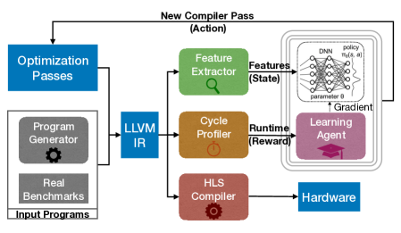
Figure 4: The block diagram of AutoPhase. The input programs are compiled to an LLVM IR using Clang/LLVM. The feature extractor and clock-cycle profiler are used to generate the input features (state) and the runtime improvement (reward), respectively from the IR. The input features and runtime improvement are fed to the deep RL agent as in input data to train on. The RL agent predicts the next best optimization passes to apply. After convergence, the HLS compiler is used to compile the LLVM IR to hardware RTL.

3.2 Clock-cycle Profiler

Once the hardware RTL is generated, one could run a hardware simulation to gather the cycle count results of the synthesized circuit. This process is quite time-consuming, hindering RL and all other optimization approaches. Therefore, we approximate cycle count using the profiler in LegUp Huang et al. (2013), which leverages the software traces and runs $20\times$ faster than hardware simulation. In LegUp, the frequency of the generated circuits is set as a compiler constraint that directs the HLS scheduling algorithm. In other words, HLS tool will always try to generate hardware that can run at a certain frequency. In our experiment setting, without loss of generality, we set the target frequency of all generated hardware to 200MHz. We experimented with lower frequencies too; the improvements were similar but the cycle counts the different algorithms achieved were better as more logic could be fitted in a single cycle.

3.3 IR Feature Extractor

Wang et al. Wang & OBoyle (2018) proposed to convert a program into an observation by extracting all the features from the program. Similarly, in addition to the LegUp backend tools, we developed analysis passes to extract 56 static features from the program, such as the number of basic blocks, branches, and instructions of various types. We use these features as partially observable states for the RL learning and hope the neural network can capture the correlation of certain combinations of these features and certain optimizations. Table 4 lists all the features used.

3.4 Random Program Generator

As a data-driven approach, RL generalizes better if we train the agent on more programs. However, there are a limited number of open-source HLS examples online. Therefore, we expand our training set by automatically generating synthetic HLS benchmarks. We first generate standard C programs using CSmith Yang et al. (2011), a random C program generator, which is originally designed to generate test cases for finding compiler bugs. Then, we develop scripts to filter out programs that take more than five minutes to run on CPU or fail the HLS compilation.

3.5 Overall Flow of AutoPhase

We integrate the compilation utilities into a simulation environment in Python with APIs similar to an OpenAI gym Brockman et al. (2016). The overall flow works as follows:

1. The input program is compiled into LLVM IR using the Clang/LLVM.

2. The IR Feature Extractor is run to extract salient program features.

3. LegUp compiles the LLVM IR into hardware RTL.

4. The Clock-cycle Profiler estimates a clock-cycle count for the generated circuit.

5. The RL agent takes the program features or the histogram of previously applied passes and the improvement in clock-cycle count as input data to train on.

6. The RL agent predicts the next best optimization passes to apply.

7. New LLVM IR is generated after the new optimization sequence is applied.

8. The machine learning algorithm iterates through steps (2)–(7) until convergence.

Note that AutoPhase uses the LLVM compiler and the passes used are listed in Table 4. However, adding support for any compiler or optimization passes in AutoPhase is very easy and straightforward. The action and state definitions must be specified again.

Table 1: LLVM Transform Passes.

0	1	2	3	4	5	6	7	8	9	10
-correlated-propagation	-scalarrepl	-lowerinvoke	-strip	-strip-nondebug	-sccp	-globalopt	-gvn	-jump-threading	-globaldce	-loop-unswitch

11	12	13	14	15	16	17	18	19	20	21
-scalarrepl-ssa	-loop-reduce	-break-crit-edges	-loop-deletion	-reassociate	-lcssa	-codegenprepare	-memcpyopt	-functionattrs	-loop-idiom	-lowerswitch

22	23	24	25	26	27	28	29	30	31	32	33
-constmerge	-loop-rotate	-partial-inliner	-inline	-early-cse	-indvars	-adce	-loop-simplify	-instcombine	-simplifycfg	-dse	-loop-unroll

34	35	36	37	38	39	40	41	42	43	44	45
-lower-expect	-tailcallelim	-licm	-sink	-mem2reg	-prune-eh	-functionattrs	-ipsccp	-deadargelim	-sroa	-loweratomic	-terminate

Table 2: Program Features.

0	Number of BB where total args for phi nodes >5	28	Number of And insts
1	Number of BB where total args for phi nodes is [1,5]	29	Number of BB’s with instructions between [15,500]
2	Number of BB’s with 1 predecessor	30	Number of BB’s with less than 15 instructions
3	Number of BB’s with 1 predecessor and 1 successor	31	Number of BitCast insts
4	Number of BB’s with 1 predecessor and 2 successors	32	Number of Br insts
5	Number of BB’s with 1 successor	33	Number of Call insts
6	Number of BB’s with 2 predecessors	34	Number of GetElementPtr insts
7	Number of BB’s with 2 predecessors and 1 successor	35	Number of ICmp insts
8	Number of BB’s with 2 predecessors and successors	36	Number of LShr insts
9	Number of BB’s with 2 successors	37	Number of Load insts
10	Number of BB’s with >2 predecessors	38	Number of Mul insts
11	Number of BB’s with Phi node # in range (0,3]	39	Number of Or insts
12	Number of BB’s with more than 3 Phi nodes	40	Number of PHI insts
13	Number of BB’s with no Phi nodes	41	Number of Ret insts
14	Number of Phi-nodes at beginning of BB	42	Number of SExt insts
15	Number of branches	43	Number of Select insts
16	Number of calls that return an int	44	Number of Shl insts
17	Number of critical edges	45	Number of Store insts
18	Number of edges	46	Number of Sub insts
19	Number of occurrences of 32-bit integer constants	47	Number of Trunc insts
20	Number of occurrences of 64-bit integer constants	48	Number of Xor insts
21	Number of occurrences of constant 0	49	Number of ZExt insts
22	Number of occurrences of constant 1	50	Number of basic blocks
23	Number of unconditional branches	51	Number of instructions (of all types)
24	Number of Binary operations with a constant operand	52	Number of memory instructions
25	Number of AShr insts	53	Number of non-external functions
26	Number of Add insts	54	Total arguments to Phi nodes
27	Number of Alloca insts	55	Number of Unary operations

4 Correlation of Passes and Program Features

Similar to the case with many deep learning approaches, explainability is one of the major challenges we face when applying deep RL to the phase-ordering challenge. To analyze and understand the correlation of passes and program features, we use random forests Breiman (2001) to learn the importance of different features. Random forest is an ensemble of multiple decision trees. The prediction made by each tree could be explained by tracing the decisions made at each node and calculating the importance of different features on making the decisions at each node. This helps us to identify the effective features and passes to use and show whether our algorithms learn informative patterns on data.

For each pass, we build two random forests to predict whether applying it would improve the circuit performance. The first forest takes the program features as inputs while the second takes a histogram of previously applied passes. To gather the training data for the forests, we run PPO with high exploration parameter on 100 randomly generated programs to generate feature–action–reward tuples. The algorithm assigns higher importance to the input features that affect the final prediction more.

4.1 Importance of Program Features

The heat map in Figure 5 shows the importance of different features on whether a pass should be applied. The higher the value is, the more important the feature is (the sum of the values in each row is one). The random forest is trained with 150,000 samples generated from the random programs. The index mapping of features and passes can be found in Tables 1 and 4. For example, the yellow pixel corresponding to feature index 17 and pass index 23 reflects that number-of-critical-edges affects the decision on whether to apply -loop-rotate greatly. A critical edge in control flow graph is an edge that is neither the only edge leaving its source block, nor the only edge entering its destination block. The critical edges can be commonly seen in a loop as a back edge so the number of critical edges might roughly represent the number of loops in a program. The transform pass -loop-rotate detects a loop and transforms a while loop to a do-while loop to eliminate one branch instruction in the loop body. Applying the pass results in better circuit performance as it reduces the total number of FSM states in a loop.

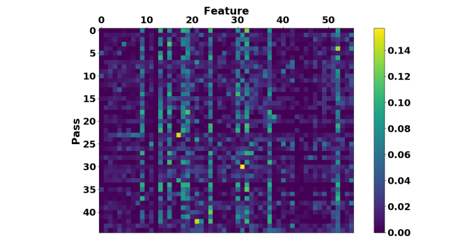
Figure 5: Heat map illustrating the importance of feature and pass indices.

Other expected behaviors are also observed in this figure. For instance, the correlation between number of branches and the transform passes -loop-simplify, -tailcallelism (which transforms calls of the current function i.e., self recursion, followed by a return instruction with a branch to the entry of the function, creating a loop), -lowerswitch (which rewrites switch instructions with a sequence of branches). Other interesting behaviors are also captured. For example, in the correlation between binary operations with a constant operand and -functionattrs, which marks different operands of a function as read-only (constant). Some correlations are harder to explain, for example, number of BitCast instructions and -instcombine, which combines instructions into fewer simpler instructions. This is actually a result of -instcombine reducing the loads and stores that call bitcast instructions for casting pointer types. Another example is number of memory instructions and -sink, where -sink basically moves memory instructions into successor blocks and delays the execution of memory until needed. Intuitively, whether to apply -sink should be dependent on whether there is any memory instruction in the program. Our last example to show is number of occurrences of constant 0 and -deadargelim, where -deadargelim helped eliminate dead/unused constant zero arguments.

Overall, we observe that all the passes are correlated to some features and are able to affect the final circuit performance. We also observe that multiple features are not effective at directing decisions and training with them could increase the variance that would result in lower prediction accuracy of our results. For example, the total number of instructions did not give a direct indication of whether applying a pass would be helpful or not. This is because sometimes more instructions could improve the performance (for example, due to loop unrolling) and eliminating unnecessary code could also improve the performance. In addition, the importance of features varies among different benchmarks depending on the tasks they perform.

4.2 Importance of Previously Applied Passes

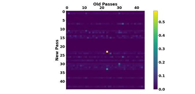
Figure 6: Heat map illustrating the importance of indices of previously applied passes and the new pass to apply.

Figure 6 illustrates the impact of previously applied passes on the new pass to apply. The higher the value is, the more important having the old pass is. From this figure, we learn that for the programs we trained on passes -scalarrepl, -gvn, -scalarrepl-ssa, -loop-reduce, -loop-deletion, -reassociate, -loop-rotate, -partial-inliner, -early-cse, -adce, -instcombine, -simplifycfg, -dse, -loop-unroll, -mem2reg, and -sroa, are more impactful on the performance compared to the rest of the passes regardless of their order in the trajectory. Point (23,23) has the highest importance in which implies that pass -loop-rotate is very helpful and should be included if not applied before. By examining thousands of the programs, we find that -loop-rotate indeed reduces the cycle count significantly. Interestingly, applying this pass twice is not harmful if the passes were given consecutively. However, giving this pass twice with some other passes between them is sometimes very harmful. Another interesting behavior our heat map captured is the fact that applying pass 33 (-loop-unroll) after (not necessarily consecutive) pass 23 (-loop-rotate) was much more useful compared to applying these two passes in the opposite order.

5 Problem Formulation

5.1 The RL Environment Definition

Assume the optimal number of passes to apply is $N$ and there are $K$ transform passes to select from in total, our search space $\mathcal{S}$ for the phase-ordering problem is $[0,K^{N})$. Given $M$ program features and the history of already applied passes, the goal of deep RL is to learn the next best optimization pass $a$ to apply that minimizes the long term cycle count of the generated hardware circuit. Note that the optimization state $s$ is partially observable in this case as the $M$ program features cannot fully capture all the properties of a program.

Action Space – we define our action space $\mathcal{A}$ as $\{a\in\mathbb{Z}:a\in[0,K)\}$ where $K$ is the total number of transform passes.

Observation Space – two types of input features were considered in our evaluation: ① program features $\mathbf{o_{f}}\in\mathbb{Z}^{M}$ listed in Table 4 and ② action history which is a histogram of previously applied passes $\mathbf{o_{a}}\in\mathbb{Z}^{K}$. After each RL step where the pass $i$ is applied, we call the feature extractor in our environment to return new $\mathbf{o_{f}}$, and update the action histogram element $o_{a_{i}}$ to $o_{a_{i}}+1$.

Reward – the cycle count of the generated circuit is reported by the clock-cycle profiler at each RL iteration. Our reward is defined as $R=c_{prev}-c_{cur}$, where $c_{prev}$ and $c_{cur}$ represent the previous and the current cycle count of the generated circuit respectively. It is possible to define a different reward for different objectives. For example, the reward could be defined as the negative of the area and thus the RL agent will optimize for the area. It is also possible to co-optimize multiple objectives (e.g., area, execution time, power, etc.) by defining a combination of different objectives.

5.2 Applying Multiple Passes per Action

An alternative to the action formulation above is to evaluate a complete sequence of passes with length $N$ instead of a single action $a$ at each RL iteration. Upon the start of training a new episode, the RL agent resets all pass indices $\mathbf{p}\in\mathbb{Z}^{N}$ to the index value $\frac{K}{2}$. For pass ${p_{i}}$ at index $i$, the next action to take is either to change to a new pass or not. By allowing positive and negative index update for each $p$, we reduced the total steps required to traverse all possible pass indices. The sub-action space $a_{i}$ for each pass is thus defined as $[-1,0,1]$. The total action space $\mathcal{A}$ is defined as $[-1,0,1]^{N}$. At each step, the RL agent predicts the updates $[a_{1},a_{2},...,a_{N}]$ to N passes, and the current optimization sequence $[p_{1},p_{2},...,p_{N}]$ is updated to $[p_{1}+a_{1},p_{2}+a_{2},...,p_{N}+a_{N}]$.

5.3 Normalization Techniques

In order for the trained RL agent to work on new programs, we need to properly normalize the program features and rewards so they represent a meaningful state among different programs. In this work, we experiment with two techniques: ① taking the logarithm of program features or rewards and, ② normalizing to a parameter from the original input program that roughly depicts the problem size. For technique ①, note that taking the logarithm of the program features not only reduces their magnitude, it also correlates them in a different manner in the neural network. Since, $w_{1}\log(o_{f_{1}})+w_{2}\log(o_{f_{2}})=log(o_{f_{1}}^{w_{1}}o_{f_{2}}^{w_{2}})$, the neural network is learning to correlate the products of features instead of a linear combination of them. For technique ②, we normalize the program features to the total number of instructions in the input program ($\mathbf{o_{f\_norm}}=\frac{\mathbf{o_{f}}}{o_{f_{51}}}$), which is feature #51 in Table 4.

6 Evaluation

To run our deep RL algorithms we use RLlib Liang et al. (2017), an open-source library for reinforcement learning that offers both high scalability and a unified API for a variety of applications. RLlib is built on top of Ray Moritz et al. (2018), a high-performance distributed execution framework targeted at large-scale machine learning and reinforcement learning applications. We ran the framework on a four-core Intel i7-4765T CPUwith a Tesla K20c GPUfor training and inference.

We set our frequency constraint in HLS to 200MHz and use the number of clock cycles reported by the HLS profiler as the circuit performance metric. In Huang et al. (2013), results showed a one-to-one correspondence between the clock cycle count and the actual hardware execution time under certain frequency constraint. Therefore, better clock cycle count will lead to better hardware performance.

6.1 Performance

To evaluate the effectiveness of various algorithms for tackling the phase-ordering problem, we run them on nine real HLS benchmarks and compare the results based on the final HLS circuit performance and the sample efficiency against state-of-the-art approaches for overcoming the phase ordering, which include random search, Greedy Algorithms Huang et al. (2013), OpenTuner Ansel et al. (2014), and Genetic Algorithms Fortin et al. (2012). These benchmarks are adapted from CHStone Hara et al. (2008) and LegUp examples. They are: adpcm, aes, blowfish, dhrystone, gsm, matmul, mpeg2, qsort, and sha. For this evaluation, the input features/rewards were not normalized, the pass length was set to 45, and each algorithm was run on a per-program basis. Table 3 lists the action and observation spaces used in all the deep RL algorithms.

Table 3: The observation and action spaces used in the different deep RL algorithms.

	RL-PPO1	RL-PPO2	RL-PPO3	RL-A3C	RL-ES
Deep RL Algorithm	PPO	PPO	PPO	A3C	ES
Observation Space	Program Features	Action History	Action History + Program Features	Program Features	Program Features
Action Space	Single-Action	Single-Action	Multiple-Action	Single-Action	Single-Action

The bar chart in Figure 7 shows the percentage improvement of the circuit performance compared to -O3 results on the nine real benchmarks from CHStone. The dots on the blue line in Figure 7 show the total number of samples for each program, which is the number of times the algorithm calls the simulator to gather the cycle count. -O0 and -O3 are the default compiler optimization levels. RL-PPO1 is a PPO explorer where we set all the rewards to 0 to test if the rewards are meaningful. RL-PPO2 is the PPO agent that learns the next pass based on a histogram of applied passes. RL-A3C is the A3C agent that learns based on the program features. Greedy performs the greedy algorithm, which always inserts the pass that achieves the highest speedup at the best position (out of all possible positions it can be inserted to) in the current sequence. RL-PPO3 uses a PPO agent and the program features but with the action space described in Section 5.2. explained in Section 5.2. OpenTuner runs an ensemble of six algorithms, which includes two families of algorithms: particle swarm optimization Kennedy (2010) and GA, each with three different crossover settings. RL-ES is similar to A3C agent that learns based on the program features, but updates the policy network using the evolution strategy instead of backpropagation. Genetic-DEAP Fortin et al. (2012) is a genetic algorithm implementation. random randomly generates a sequence of 45 passes at once instead of sampling them one-by-one.

From Greedy, we see that always adding the pass in the current sequence that achieves the highest reward leads to sub-optimal circuit performance. RL-PPO2 achieves higher performance than RL-PPO1, which shows that the deep RL captures useful information during training. Using the histogram of applied passes results in better sample efficiency, but using the program features with more samples results in a slightly higher speedup. RL-PPO2, for example, at the minor cost of 4% lower speedup, achieves 50$\times$ more sample efficiency than OpenTuner. Using ES to update the policy is supposed to be more sample efficient for problems with sparse rewards like ours, however, our experiments did not benefit from that. Furthermore, RL-PPO3 with multiple action updates achieves a higher speedup than the other deep RL algorithms with a single action. One reason for that is the ability of RL-PPO3 to explore more passes per compilation as it applies multiple passes simultaneously in between every compilation. On the other hand, the other deep RL algorithms apply a single pass at a time.

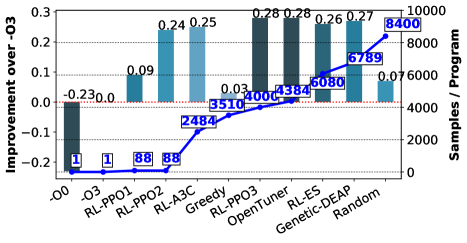
Figure 7: Circuit Speedup and Sample Size Comparison.

6.2 Generalization

With deep RL, the search should benefit from prior knowledge learned from other different programs. This knowledge should be transferable from one program to another. For example, as discussed in section 4 applying pass -loop-rotate is always beneficial, and -loop-unroll should be applied after -loop-rotate. Note that the black-box search algorithms, such as OpenTuner, GA, and greedy algorithms, cannot generalize. For these algorithms, rerunning a new search with many compilations is necessary for every new program, as they do not learn any patterns from the programs to direct the search and can be viewed as a smart random search.

To evaluate how generalizable deep RL could be with different programs and whether any prior knowledge could be useful, we train on 100 randomly-generated programs using PPO. Random programs are used for transfer learning due to lack of sufficient benchmarks and because it is the worst-case scenario, i.e., they are very different from the programs that we use for inference. The improvement can be higher if we train on programs that are similar to the ones we inference on. We train a network with $256\times 256$ fully connected layers and use the histogram of previously applied passes concatenated to the program features as the observation and passes as actions.

As described in Section 5.3, we experiment with two normalization techniques for the program features: ① taking the logarithm of all the program features and ② normalizing the program features to the total number of instructions in the program. In each pass sequence, the intermediate reward was defined as the logarithm of the improvement in cycle count after applying each pass. The logarithm was chosen so that the RL agent will not give much larger weights to big rewards from programs with longer execution time. Three approaches were evaluated: filtered-norm1 uses the filtered (based on the analysis in Section 4 where we only keep the important features and passes) program features and passes from Section with normalization technique ①, original-norm2 uses all the program features and passes with normalization technique ②, and filtered-norm2 uses the filtered program features and passes from Section 4 with normalization technique ②. Filtering the features and passes might not be ideal, especially when different programs have different feature characteristics and impactful passes. However, reducing the number of features and passes helps to reduce variance among all programs and significantly narrow the search space.

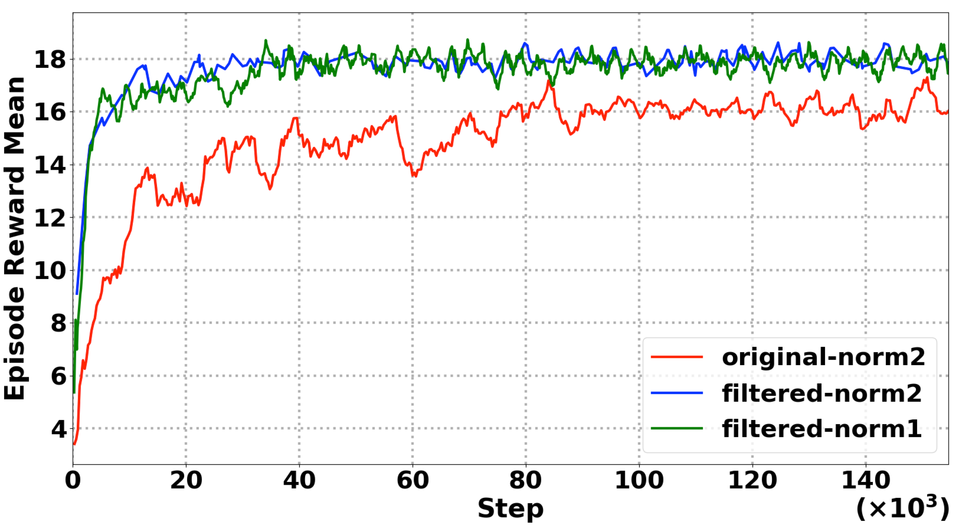
Figure 8: Episode reward mean as a function of step for the original approach where we use all the program features and passes and for the filtered approach where we filter the passes and features (with different normalization techniques). Higher values indicate faster circuit speed.

Figure 8 shows the episode reward mean as a function of the step for the three approaches. We observe that filtered-norm2 and filtered-norm1 converge much faster and achieve a higher episode reward mean than original-norm2, which uses all the features and passes. At roughly 8,000 steps the filtered-norm2 and filter-norm1 already achieve a very high episode reward mean, with minor improvements in later steps. Furthermore, the episode reward mean of the filtered approaches is still higher than that of original-norm2 even when we allowed it to train for 20 times more steps (i.e., 160,000 steps). This indicates that filtering the features and passes significantly improved the learning process. All three approaches learned to always apply pass -loop-rotate, and -loop-unroll after -loop-rotate. Another useful pass that the three approaches learned to apply is -loop-simplify, which performs several transformations to transform natural loops into a simpler form that enables subsequent analyses and transformations.

We now compare the generalization results of filtered-norm2 and filtered-norm1 with the other black-box algorithms. We use 100 randomly-generated programs as the training set and nine real benchmarks from CHStone as the testing set for the deep RL-based methods. With the state-of-the-art black-box algorithms, we first search for the best pass sequences that achieved the lowest aggregated hardware cycle counts for the 100 random programs and then directly apply them to the nine test set programs. In Figure 9, the bar chart shows the percentage improvement of the circuit performance compared to -O3 on the nine real benchmarks, the dots on the blue line show the total number of samples each inference takes for one new program.

This evaluation shows that the deep RL-based inference achieves higher speedup than the predetermined sequences produced by the state-of-the-art black-box algorithms for new programs. The predetermined sequences that are overfitted to the random programs can cause poor performance in unseen programs (e.g., -24% for Genetic-DEAP). Besides, normalization technique ② works better compared to normalization technique① for deep RL generalization (4% vs 3% speedup). This indicates that normalizing the different instructions to the total number of instructions i.e., the distribution of the different instructions in Technique ② represents more universal characteristics across different programs, while taking the log in Technique ① only suppresses the value ranges of different program features. Furthermore, when we use other 12,874 randomly generated programs as the testing set with filtered-norm2, the speedup is 6% compared to -O3.

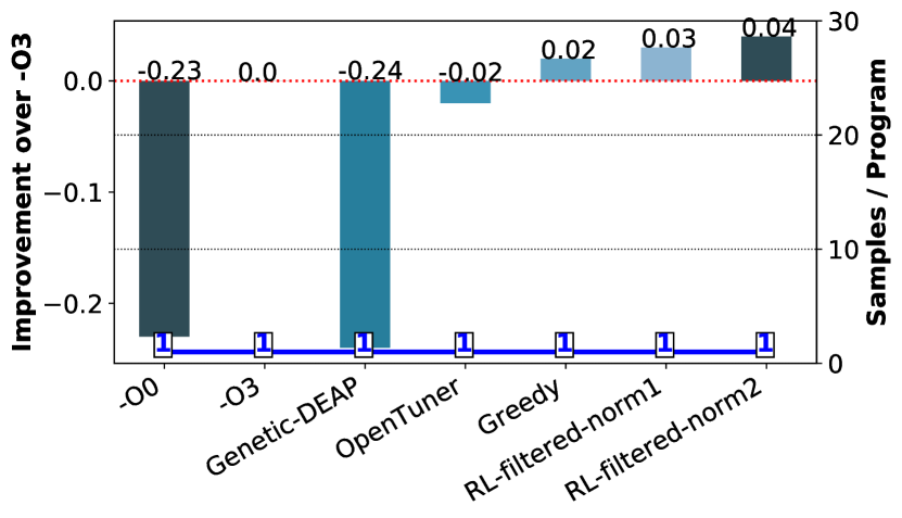
Figure 9: Circuit Speedup and Sample Size Comparison for deep RL Generalization.

7 Conclusions

In this paper, we propose an approach based on deep RL to improve the performance of HLS designs by optimizing the order in which the compiler applies optimization phases. We use random forests to analyze the relationship between program features and optimization passes. We then leverage this relationship to reduce the search space by identifying the most likely optimization phases to improve the performance, given the program features. Our RL based approach achieves 28% better performance than compiling with the -O3 flag after training for a few minutes, and a 24% improvement after training for less than a minute. Furthermore, we show that unlike prior work, our solution shows potential to generalize to a variety of programs. While in this paper we have applied deep RL to HLS, we believe that the same approach can be successfully applied to software compilation and optimization. Going forward, we envision using deep RL techniques to optimize a wide range of programs and systems.

Table 4: Program features: number of different operations.

Number of BB where total args for phi nodes >5	Number of And insts
Number of BB where total args for phi nodes is [1,5]	Number of BB’s with instructions between [15,500]
Number of BB’s with 1 predecessor	Number of BB’s with less than 15 instructions
Number of BB’s with 1 predecessor and 1 successor	Number of BitCast insts
Number of BB’s with 1 predecessor and 2 successors	Number of Br insts
Number of BB’s with 1 successor	Number of Call insts
Number of BB’s with 2 predecessors	Number of GetElementPtr insts
Number of BB’s with 2 predecessors and 1 successor	Number of ICmp insts
Number of BB’s with 2 predecessors and successors	Number of LShr insts
Number of BB’s with 2 successors	Number of Load insts
Number of BB’s with >2 predecessors	Number of Mul insts
Number of BB’s with Phi node # in range (0,3]	Number of Or insts
Number of BB’s with more than 3 Phi nodes	Number of PHI insts
Number of BB’s with no Phi nodes	Number of Ret insts
Number of Phi-nodes at beginning of BB	Number of SExt insts
Number of branches	Number of Select insts
Number of calls that return an int	Number of Shl insts
Number of critical edges	Number of Store insts
Number of edges	Number of Sub insts
Number of occurrences of 32-bit integer constants	Number of Trunc insts
Number of occurrences of 64-bit integer constants	Number of Xor insts
Number of occurrences of constant 0	Number of ZExt insts
Number of occurrences of constant 1	Number of basic blocks
Number of unconditional branches	Number of instructions (of all types)
Number of Binary operations with a constant operand	Number of memory instructions
Number of AShr insts	Number of non-external functions
Number of Add insts	Total arguments to Phi nodes
Number of Alloca insts	Number of Unary operations

Table 5: The cycles for searching the best three passes using the different search algorithms for different tasks.

	Cycles
Task	RL	-O3	random	Greedy	Genetic	No Opt.
aes	9003	9181	9003	11765	9003	11913
adpcm	13707	16244	15837	Error	13707	40430
bf	180050	187327	185250	185269	180050	197395
jpeg	1296330	1313851	1318382	1239409	1296330	1474020
mpeg2	8356	8260	8356	8469	8356	10485
sha driver	209154	226234	209154	222024	209154	296387
gsm	6168	6491	6172	6869	6168	7810
fir	1850	1768	1850	2598	1850	2172
dhry	7767	5912	8793	8793	7767	9194
qsort	49948	49948	53733	54347	49948	56092
mm	33244	33244	33244	33244	33244	42085
dfadd	726	726	726	726	726	773

Table 6: The cycles for searching the best $12$ passes using the different search algorithms for different tasks.

	Cycles
Task	DQN 12-steps	DQN 4-steps	DQN 1-step	PG	-O3	random	Greedy	Genetic	No Opt.
aes	9003	9003	11693	9003	9181	9003	9003	9003	11913
adpcm	8501	13707	36537	13657	16244	14463	13607	8501	40430
bf	180054	180050	180069	180050	187327	180054	180050	180054	197395
jpeg	1305864	1305583	1295373	1296330	1313851	1324660	1305583	1305775	1474020
mpeg2	8356	8356	8392	8280	8260	8280	8274	8280	10485
sha driver	209154	209154	222024	209154	226234	209168	209154	209154	269387
gsm	5849	5849	6696	6168	6491	6168	5849	5849	7810
fir	1850	1850	1850	1850	1768	1850	1850	1850	2172
dhry	6162	7955	7767	7767	5912	5974	7767	5974	9194
qsort	49948	49948	49889	49948	49948	49889	49889	49948	56092
mm	33244	33244	33244	33244	33244	33244	33244	33244	42085
dfadd	726	726	726	726	726	726	726	726	773

References

- Agakov et al. (2006) Agakov, F., Bonilla, E., Cavazos, J., Franke, B., Fursin, G., O’Boyle, M. F., Thomson, J., Toussaint, M., and Williams, C. K. Using machine learning to focus iterative optimization. In Proceedings of the International Symposium on Code Generation and Optimization, pp. 295–305. IEEE Computer Society, 2006.
- Almagor et al. (2004) Almagor, L., Cooper, K. D., Grosul, A., Harvey, T. J., Reeves, S. W., Subramanian, D., Torczon, L., and Waterman, T. Finding effective compilation sequences. ACM SIGPLAN Notices, 39(7):231–239, 2004.
- Ansel et al. (2014) Ansel, J., Kamil, S., Veeramachaneni, K., Ragan-Kelley, J., Bosboom, J., O’Reilly, U.-M., and Amarasinghe, S. Opentuner: An extensible framework for program autotuning. In Proceedings of the 23rd international conference on Parallel architectures and compilation, pp. 303–316. ACM, 2014.
- Bellman (1957) Bellman, R. A markovian decision process. In Journal of Mathematics and Mechanics, pp. 679–684, 1957.
- Breiman (2001) Breiman, L. Random forests. Machine learning, 45(1):5–32, 2001.
- Brockman et al. (2016) Brockman, G., Cheung, V., Pettersson, L., Schneider, J., Schulman, J., Tang, J., and Zaremba, W. Openai gym, 2016.
- Canis et al. (2013) Canis, A., Choi, J., Aldham, M., Zhang, V., Kammoona, A., Czajkowski, T., Brown, S. D., and Anderson, J. H. Legup: An open-source high-level synthesis tool for fpga-based processor/accelerator systems. ACM Transactions on Embedded Computing Systems (TECS), 13(2):24, 2013.
- Conti et al. (2018) Conti, E., Madhavan, V., Such, F. P., Lehman, J., Stanley, K., and Clune, J. Improving exploration in evolution strategies for deep reinforcement learning via a population of novelty-seeking agents. In Advances in Neural Information Processing Systems, pp. 5032–5043, 2018.
- Fortin et al. (2012) Fortin, F.-A., De Rainville, F.-M., Gardner, M.-A., Parizeau, M., and Gagné, C. DEAP: Evolutionary algorithms made easy. Journal of Machine Learning Research, 13:2171–2175, jul 2012.
- Fursin et al. (2011) Fursin, G., Kashnikov, Y., Memon, A. W., Chamski, Z., Temam, O., Namolaru, M., Yom-Tov, E., Mendelson, B., Zaks, A., Courtois, E., et al. Milepost gcc: Machine learning enabled self-tuning compiler. International journal of parallel programming, 39(3):296–327, 2011.
- Goldberg (2006) Goldberg, D. E. Genetic algorithms. Pearson Education India, 2006.
- Haj-Ali et al. (2019a) Haj-Ali, A., Ahmed, N. K., Willke, T., Shao, S., Asanovic, K., and Stoica, I. Learning to vectorize using deep reinforcement learning. In Workshop on ML for Systems at NeurIPS, December 2019a.
- Haj-Ali et al. (2019b) Haj-Ali, A., K. Ahmed, N., Willke, T., Gonzalez, J., Asanovic, K., and Stoica, I. A view on deep reinforcement learning in system optimization. arXiv preprint arXiv:1908.01275, 2019b.
- Haj-Ali et al. (2020) Haj-Ali, A., Ahmed, N. K., Willke, T., Shao, S., Asanovic, K., and Stoica, I. Neurovectorizer: End-to-end vectorization with deep reinforcement learning. International Symposium on Code Generation and Optimization (CGO), February 2020.
- Hara et al. (2008) Hara, Y., Tomiyama, H., Honda, S., Takada, H., and Ishii, K. CHstone: A benchmark program suite for practical c-based high-level synthesis. In Circuits and Systems, 2008. ISCAS 2008. IEEE International Symposium on, pp. 1192–1195, 2008.
- Huang et al. (2013) Huang, Q., Lian, R., Canis, A., Choi, J., Xi, R., Brown, S., and Anderson, J. The effect of compiler optimizations on high-level synthesis for fpgas. In Field-Programmable Custom Computing Machines (FCCM), 2013 IEEE 21st Annual International Symposium on, pp. 89–96. IEEE, 2013.
- Huang et al. (2015) Huang, Q., Lian, R., Canis, A., Choi, J., Xi, R., Calagar, N., Brown, S., and Anderson, J. The effect of compiler optimizations on high-level synthesis-generated hardware. ACM Transactions on Reconfigurable Technology and Systems (TRETS), 8(3):14, 2015.
- Huang et al. (2019) Huang, Q., Haj-Ali, A., Moses, W., Xiang, J., Stoica, I., Asanovic, K., and Wawrzynek, J. Autophase: Compiler phase-ordering for hls with deep reinforcement learning. In 2019 IEEE 27th Annual International Symposium on Field-Programmable Custom Computing Machines (FCCM), pp. 308–308. IEEE, 2019.
- Intel (2019) Intel. Intel High-Level Synthesis Compiler, 2019. URL {https://www.intel.com/content/www/us/en/software/programmable/quartus-prime/hls-compiler.html}.
- Kaelbling et al. (1996) Kaelbling, L. P., Littman, M. L., and Moore, A. W. Reinforcement learning: A survey. In Reinforcement learning: A survey, volume 4, pp. 237–285, 1996.
- Kennedy (2010) Kennedy, J. Particle swarm optimization. Encyclopedia of machine learning, pp. 760–766, 2010.
- Kulkarni & Cavazos (2012) Kulkarni, S. and Cavazos, J. Mitigating the compiler optimization phase-ordering problem using machine learning. In Proceedings of the ACM International Conference on Object Oriented Programming Systems Languages and Applications, OOPSLA ’12, 2012.
- Lattner & Adve (2004) Lattner, C. and Adve, V. Llvm: A compilation framework for lifelong program analysis & transformation. In International Symposium on Code Generation and Optimization, 2004. CGO 2004., pp. 75–86. IEEE, 2004.
- Liang et al. (2017) Liang, E., Liaw, R., Moritz, P., Nishihara, R., Fox, R., Goldberg, K., Gonzalez, J. E., Jordan, M. I., and Stoica, I. Rllib: Abstractions for distributed reinforcement learning. arXiv preprint arXiv:1712.09381, 2017.
- Mnih et al. (2016) Mnih, V., Badia, A. P., Mirza, M., Graves, A., Lillicrap, T., Harley, T., Silver, D., and Kavukcuoglu, K. Asynchronous methods for deep reinforcement learning. In International conference on machine learning, pp. 1928–1937, 2016.
- Moritz et al. (2018) Moritz, P., Nishihara, R., Wang, S., Tumanov, A., Liaw, R., Liang, E., Elibol, M., Yang, Z., Paul, W., Jordan, M. I., et al. Ray: A distributed framework for emerging AI applications. In 13th USENIX Symposium on Operating Systems Design and Implementation (OSDI 18), pp. 561–577, 2018.
- Muchnick (1997) Muchnick, S. S. Advanced compiler design and implementation. In Advanced Compiler Design and Implementation. Morgan Kaufmann, 1997.
- Pan & Eigenmann (2006) Pan, Z. and Eigenmann, R. Fast and effective orchestration of compiler optimizations for automatic performance tuning. In Proceedings of the International Symposium on Code Generation and Optimization, pp. 319–332. IEEE Computer Society, 2006.
- Ross et al. (2011) Ross, S., Gordon, G., and Bagnell, D. A reduction of imitation learning and structured prediction to no-regret online learning. In Proceedings of the fourteenth international conference on artificial intelligence and statistics, pp. 627–635, 2011.
- Salimans et al. (2017) Salimans, T., Ho, J., Chen, X., Sidor, S., and Sutskever, I. Evolution strategies as a scalable alternative to reinforcement learning. arXiv preprint arXiv:1703.03864, 2017.
- Schulman et al. (2017) Schulman, J., Wolski, F., Dhariwal, P., Radford, A., and Klimov, O. Proximal policy optimization algorithms. arXiv preprint arXiv:1707.06347, 2017.
- Stephenson et al. (2003) Stephenson, M., Amarasinghe, S., Martin, M., and O’Reilly, U.-M. Meta optimization: Improving compiler heuristics with machine learning. In Proceedings of the ACM SIGPLAN 2003 Conference on Programming Language Design and Implementation, PLDI ’03, 2003.
- Sutton & Barto (1998) Sutton, R. S. and Barto, A. G. Introduction to reinforcement learning, volume 135. MIT press Cambridge, 1998.
- Sutton et al. (2000) Sutton, R. S., McAllester, D. A., Singh, S. P., and Mansour, Y. Policy gradient methods for reinforcement learning with function approximation. In Advances in neural information processing systems, pp. 1057–1063, 2000.
- Triantafyllis et al. (2003) Triantafyllis, S., Vachharajani, M., Vachharajani, N., and August, D. I. Compiler optimization-space exploration. In Proceedings of the international symposium on Code generation and optimization: feedback-directed and runtime optimization, pp. 204–215. IEEE Computer Society, 2003.
- Wang & OBoyle (2018) Wang, Z. and OBoyle, M. Machine learning in compiler optimization. In Machine Learning in Compiler Optimization, volume 106, pp. 1879–1901, Nov 2018.
- Xilinx (2019) Xilinx. Vivado High-Level Synthesis, 2019. URL {https://www.xilinx.com/products/design-tools/vivado/integration/esl-design.html}.
- Yang et al. (2011) Yang, X., Chen, Y., Eide, E., and Regehr, J. Finding and understanding bugs in c compilers. In ACM SIGPLAN Notices, volume 46, pp. 283–294. ACM, 2011.