Graph3S: A Simple, Speedy and Scalable Distributed Graph Processing System

Abstract

Graph is a ubiquitous structure in many domains. The rapidly increasing data volume calls for efficient and scalable graph data processing. In recent years, designing distributed graph processing systems has been an increasingly important area to fulfil the demands of processing big graphs in a distributed environment. Though a variety of distributed graph processing systems have been developed, very little attention has been paid to achieving a good combinational system performance in terms of usage simplicity, efficiency and scalability. To contribute to the study of distributed graph processing system, this work tries to fill this gap by designing a simple, speedy and scalable system. Our observation is that enforcing the communication flexibility of a system leads to the gains of both system efficiency and scalability as well as simple usage. We realize our idea in a system $\mathsf{Graph3S}$ and conduct extensive experiments with diverse algorithms over big graphs from different domains to test its performance. The results show that, besides simple usage, our system has outstanding performance over various graph algorithms and can even reach up to two orders of magnitude speedup over existing in-memory systems when applying to some algorithms. Also, its scalability is competitive to disk-based systems and even better when less machines are used.

1 Introduction

Graph is a ubiquitous structure representing entities and their relationships. It is applied in many areas including social network, web graph, road network, biology and so on. Basic graph problems like Pagerank, connected component, graph coloring, etc., are playing fundamental roles in many real-life applications. Efficiently processing graph data is essential in both research and practice. With the dramatic increasing data volume, a lot of research interests have been shown on designing distributed graph processing systems to process big graphs in a distributed environment[8, 9, 10, 11, 21, 24, 43, 44, 49].

Table 1: System Comparison

System	Simplicity	Efficiency	Scalability	Flexibility
$\mathsf{Pregel}$	$\star$ $\star$ $\star$	$\star$ $\star$ $\star$	$\star$ $\star$ $\star$	$\star$ $\star$ $\star$ $\star$ $\star$
$\mathsf{Pregel+}$	$\star$ $\star$	$\star$ $\star$ $\star$	$\star$ $\star$	$\star$ $\star$ $\star$ $\star$ $\star$
$\mathsf{PowerGraph}$	$\star$ $\star$ $\star$	$\star$ $\star$ $\star$	$\star$	$\star$ $\star$ $\star$ $\star$
$\mathsf{Blogel}$	$\star$	$\star$ $\star$ $\star$	$\star$ $\star$	$\star$ $\star$ $\star$ $\star$ $\star$
$\mathsf{GraphD}$	$\star$ $\star$	$\star$	$\star$ $\star$ $\star$ $\star$ $\star$	$\star$ $\star$ $\star$ $\star$ $\star$
$\mathsf{Graph3S}$	$\star$ $\star$ $\star$ $\star$ $\star$	$\star$ $\star$ $\star$ $\star$ $\star$	$\star$ $\star$ $\star$ $\star$ $\star$	$\star$ $\star$ $\star$ $\star$

Though many distributed graph processing systems have been proposed, we find that not much effort has been put in achieving a good combinational performance in terms of system usage simplicity, efficiency and scalability. Table 1 shows the scores in terms of each aspect of existing representative systems. The scores are relatively given among the systems based on our experimental results. Among them, $\mathsf{Pregel}$ [24], $\mathsf{Pregel+}$ [44], $\mathsf{PowerGraph}$ [12, 21] and $\mathsf{GraphD}$ [47] are vertex-centric systems. $\mathsf{Blogel}$ [43] is a block-centric system. All these systems are in-memory systems except $\mathsf{GraphD}$ which is an out-of-core system. From the table, we can see that none of the existing systems claims a robust performance in the combination of system simplicity, efficiency and scalability, which are all important to end users when processing big graph data. The unsatisfactory situation is understandable since many works focus on improving system efficiency by introducing complicated techniques with more APIs to be implemented by users. For example, $\mathsf{Pregel+}$ implements Google’s popular model $\mathsf{Pregel}$ with message reduction and load balancing techniques to improve system efficiency. However, the proposed two modes of $\mathsf{Pregel+}$ require users to not only have the related knowledge to choose between them for different applications and graphs so as to achieve best performance, but also implement corresponding APIs in different modes. Hence, from system usage perspective, $\mathsf{Pregel+}$ is more complicated than $\mathsf{Pregel}$. On the other hand, some studies aim at improving system scalability but usually sacrifices system efficiency. For instance, $\mathsf{GraphD}$ aims to improve scalability on top of $\mathsf{Pregel+}$ by adopting a semi-streaming model. However, the system efficiency becomes weak because many disk accesses are involved. Even though some techniques like ID recoding are proposed to compensate the efficiency sacrifice, not only more APIs are needed and the usage simplicity is thus decreased, but also the technique is only applicable to certain kinds of algorithms. Moreover, its efficiency is still not comparable to in-memory systems. As a result, to design a distributed graph processing system that is simple to use and with no compromises in efficiency and scalability is challenging and yet to be studied. In this paper, we aim to tackle this problem by designing a Simple, Speedy and Scalable distributed graph processing system, named $\mathsf{Graph3S}$.

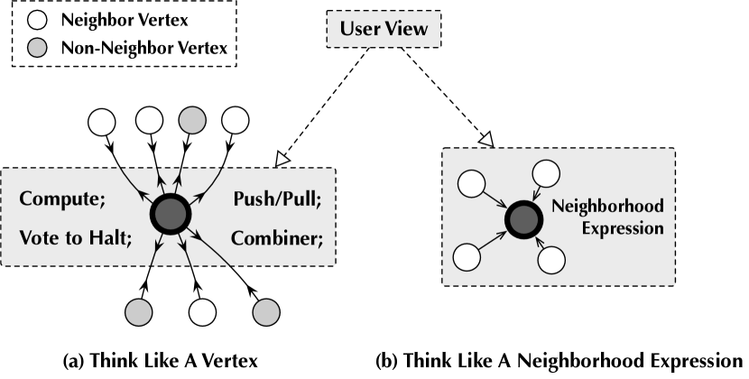
Figure 1: Flexibility $\Rightarrow$ {Simplicity + Efficiency + Scalability}

Observation. We find that a vertex in existing systems is free to communicate with any vertex in a given graph including its neighbor and non-neighbor vertices as shown in Figure 1(a). We call the set of vertices that a vertex can communicate with in a system as the $communication$ $flexibility$ of the system. Our main idea is to trade the communication flexibility of a system for all three of simplicity, efficiency and scalability. In particular, we propose to enforce the communication range of a vertex in $\mathsf{Graph3S}$ just as its neighborhood as shown in Figure 1(b). This enforcement weakens the flexibility of our system, which means $\mathsf{Graph3S}$ only supports graph processing algorithms where a vertex just communicates with its neighbors like Pagerank, connected component, graph coloring and k-core decomposition. While existing systems also support algorithms where a vertex communicates with any other vertex like minimum spanning forest algorithm discussed in [44]. However, our enforcement is acceptable because we can implement all current benchmark algorithms evaluated by the existing distributed graph processing systems. More importantly, this enforcement leads to three-fold benefits.

Easy of programming. The flexible communication in existing systems requires their implementations to expose communication tasks as well as vertex state management to users so that a user can program the communication behaviours of a vertex, whereas the enforcement in $\mathsf{Graph3S}$ makes it possible that users only need to provide a computation function based on which a vertex compute its values. We call this function as a neighborhood expression as shown in Figure 1(b), because it only involves the neighbor vertices. We name the simple programming model as Think Like a Neighborhood Expression ($\mathsf{TLNE}$) because users of $\mathsf{Graph3S}$ only provide a neighborhood expression. We save a vertex’s neighborhood information locally in a distributed environment. Thus, with the neighborhood expression provided by a user, the system can automatically finish all the jobs. This will greatly simplify the workload on the user side considering users of existing systems need to take care of not only computation, but also communication, vertex state maintenance, and many optimization realizations (Figure 1(a)). Algorithm 1 shows the implementation code of breadth-first search ($\mathsf{BFS}$) on $\mathsf{Graph3S}$. The distance $dis$ of a vertex $v$ to source vertex $s$ is updated as the $min\{u.dis+1\}$ where $u$ is a in-neighbor of $v$. The neighborhood expression is designated in line 3-4. By contrast, in existing systems, a user also needs to design the functions of pushing/pulling messages, when to start/stop computation, combiners and so on [21, 24, 43, 44].

Input: A given dataset $dataset$; source vertex $s$

Output: The distance $V.dis$ of each vertex $V$ to $s$

1

2 Vertex V(int, dis);

3 Graph G($dataset$);

4

5G.ITER_N(V.dis= (ID==$s$) ? 0 : $\mathsf{INT\_MAX}$, 1);

6 G.ITER(EACH_IN V.dis=min(V.dis, INB.dis+1));

Algorithm 1 BFS on $\mathsf{Graph3S}$

Efficiency. The enforcement also leads to efficient implementations. Firstly, different from pushing/pulling required multiple vertex attributes in existing systems, only changed vertex attributes, we name as $critical$ $attributes$, are synchronized in $\mathsf{Graph3S}$ which reduces communication cost. Secondly, a dual neighbor index is designed to accelerate vertex computation and activation procedure. We also propose a $self$-$adaptive$ $activation$ mechanism based on the dual neighbor index which further improves the efficiency of $\mathsf{Graph3S}$. Note that these techniques are not feasible if a vertex communicates with both neighbors and non-neibors considering system scalability.

Scalability. Since the applications in $\mathsf{Graph3S}$ only need neighborhood information, we adopt a semi-caching model in $\mathsf{Graph3S}$ where vertex information is saved in memory and neighborhood information is saved on disk. This is practical because vertex values are frequently and randomly accessed and edge information can be scanned linearly. Besides, edge information usually has a much higher space cost $O(n^{2})$ than that of vertex information $O(n)$ where $n$ is the number of vertices in a given graph.

Extensive experiments comparing our system with popular state-of-the-art distributed graph processing systems validate these benefits of our enforcement in $\mathsf{Graph3S}$. Note that the lack of diversity in applications for evaluating system usability and performance is a concern for existing works [15]. Therefore, in this paper, despite commonly used similar and single-stage algorithms, we also include more complex and multi-stage algorithms to test the system performance. We implement $9$ popular graph algorithms on compared systems and evaluate them over six large-scale real datasets from different domains with various characteristics.

Contribution. In this paper, our principle contributions are shown as follows.

• We study the simplicity, efficiency and scalability of a distributed graph processing system by trading communication flexibility.

• We design a simple, speedy and scalable system $\mathsf{Graph3S}$ to implement our idea.

• We conduct extensive experiments to prove the good performance of our system compared to existing systems.

Outline. The remainder of this paper is organised as follows: Section 2 reviews the existing work on graph processing systems. Section 3 introduces our system and implementation techniques. In Section 4, extensive experiments over real-life datasets are conducted and results are reported. Section 5 concludes this paper.

2 Related Work

This section reports our review of existing graph processing systems. Based on the given graph is processed in a single machine or a cluster, the existing systems could be categorised as either single-machine or distributed systems.

2.1 Single-Machine (shared-memory) Systems

Single-machine graph processing systems store and process a given graph in a single machine. There are some existing works on single-machine graph processing systems [5, 6, 14, 17, 26, 28, 36, 37]. Ligra [31] adopts a lightweight graph processing framework with two mapping modes: vertex and edge. It dynamically switches between these two modes based on vertex subset density. The framework is efficient on graph traversal algorithms like BFS. GraphChi[17] is a vertex-centric, disk-based system designed for processing large graphs in a single machine. It adopts a method called parallel sliding windows (PSW) for processing large graphs from disks with a very small number of non-sequential accesses to the disk. X-Stream[28] is an edge-centric single-machine system for large-scale graphs by streaming edge data from disk. TurboGraph [14] is a disk-based graph engine that introduces the pin-and-slide model to perform generalized matrix-vector multiplication on a single machine. PathGraph [48] is a path-centric graph processing system which partitions a large graph into tree-based partitions and store trees in a DFS order. VENUS[5] adopts a vertex-centric streamlined processing model and proposes a new graph storage scheme, v-shards, with two different implementation algorithms. FlashGraph [7] adopts semi-external memory model for graphs stored on fast I/O device like SSD. In GridGraph [52], graphs are partitioned into 1D-partitioned vertex chunks and 2D-partitioned edge blocks. A 2-level hierarchical partitioning is applied to ensure data locality and reduce disk I/O. NXgraph[6] proposes a new structure called Destination-Sorted Sub-Shard to ensure graph data locality and enable fine-grained scheduling. It introduces three updating strategies and adapts to choose the fastest strategy.

Single-machine graph processing systems have high efficiency because of communication cost saving and fast convergence. However, the disadvantage is their weak scalability due to limited hardware sources. Considering system scalability, in this paper, we aim at a distributed graph processing system which can avoid out-of-memory error by increasing the number of machines until input graph could fit within distributed memory machines.

2.2 Distributed (shared-nothing) Systems

For distributed graph processing systems, a given graph is usually partitioned to different machines in a cluster. According to the programming model, existing distributed systems could be divided into vertex-centric (or edge-centric) and subgraph-centric (or block-centric) systems.

Think Like A Vertex Most existing distributed graph systems adopt the ”think like a v ertex” ($\mathsf{TLV}$) model where users can design an application by specifying the behaviour of a vertex. Malewick et al. [24] first proposed this model and designed a $\mathsf{TLV}$ system named $\mathsf{Pregel}$ which is based on the bulk synchronous parallel (BSP) model [35]. The BSP model consists of iterations. Inside each iteration, active vertices conduct computation as well as communication with other vertices. Giraph[11] is an open-source implementation of $\mathsf{Pregel}$ in Java. GPS [29] presents an optimization technique, large adjacency list partitioning, for high-degree vertices. Yan et al. [44] designed a system named $\mathsf{Pregel+}$ implementing $\mathsf{Pregel}$ with message reduction and load balancing techniques. Zhu et al. [51] present a distributed system Gemini based on a hybrid push-pull computation model. GraphLab (PowerGraph) [12, 21] adopts the vertex-cut partition schema and supports both synchronous and asynchronous computation modes. It adopts a Gather, Apply, and Scatter (GAS) programming model where users still think like a vertex.

Because distributed in-memory systems provide high efficiency but are weak in scalability, some distributed external-memory systems are proposed to compensate [1, 2, 16, 47]. TurboGraph++ [16] extends a single out-of-core graph processing system TurboGraph [14] to a distributed environment. Yan et al. proposed an out-of-core distributed graph system $\mathsf{GraphD}$ [47] based on a semi-streaming model where vertex states are stored in memory and edges and messages are streamed from disk.

There are also some studies on general graph processing system optimization techniques [3, 8, 13, 20, 30, 32, 38, 7, 50]. Salihoglu et al. [30] proposed some optimization techniques to implement algorithms efficiently on $\mathsf{Pregel}$-like systems. Wang et al. [38] designed an automatic switching mechanism between push and pull computation models to reduce I/O costs on disk data. Song et al. [32] put forward a redundancy reduction strategy to achieve high-performance graph analytics by using graph structure. The other works focus on improving system efficiency through new hardwares, like SSDs, GPUs[20, 7, 50]. We leave these optimization works out of comparison in our study.

Think Like A Subgraph There is another category of graph processing systems that allows users to program with a subgraph[4, 10, 27, 33, 34, 43]. Yan et al. [43] designed $\mathsf{Blogel}$ where each connected subgraph is a block and users program functions for blocks. NScale [27] and Arabesque [33] adopt the k-hop neighborhood-centric model based on MapReduce framework. G-Miner [4] models subgraph mining problems as independent tasks and provides a task-based pipeline to asynchronously process CPU, Network, Disk I/O operations for efficiency.

Despite which model an existing system adopts, users still need to implement multiple functions to specify the behaviours of a vertex or a subgraph. These usually include computation and communication functions, optimization techniques and so on. However, as validated by our experiments, our system is not only simple to use but also shows good efficiency and scalability over different algorithms.

3 The System

To meet the requirement of a good system in terms of simplicity, efficiency and scalability, we design a new system named $\mathsf{Graph3S}$. In this section, we first provide the overview of $\mathsf{Graph3S}$, followed by the detailed introduction of proposed techniques about the Simple, Speedy and Scalable aspects of $\mathsf{Graph3S}$.

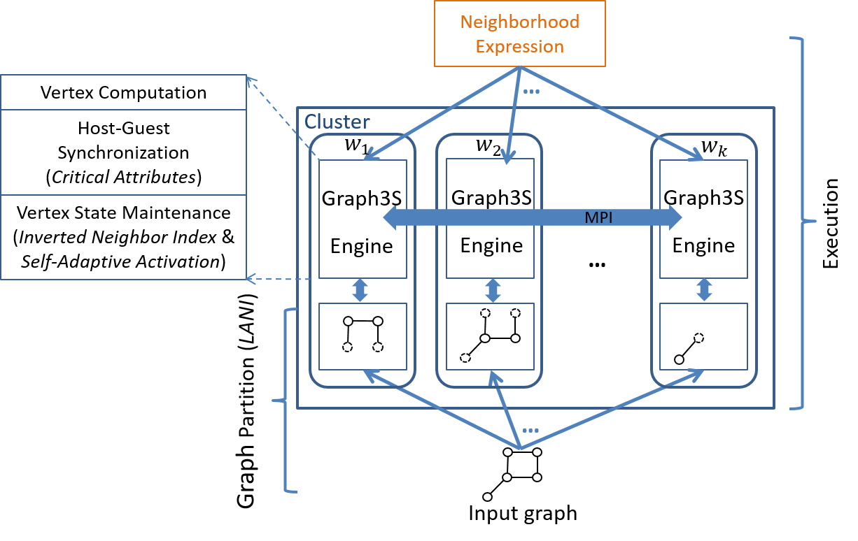
Figure 2: $\mathsf{Graph3S}$ overview.

3.1 Overview

Figure 2 shows the overview of $\mathsf{Graph3S}$. A user only needs to provide a neighborhood expression based on which a vertex computes its value to the system. Then the rest of the work is automatically done by $\mathsf{Graph3S}$. Input graph is partitioned to different workers in a hashing way. We adopt the Bulk Synchronous Parallel ($\mathsf{BSP}$) model in $\mathsf{Graph3S}$ engine. BSP is based on iterative supersteps (iterations). Vertex computation, communication (Host-Guest Synchronization), and vertex state maintenance happen in each superstep with synchronization barrier occurring at the end of each superstep.

3.2 Simple

Now we introduce how easily a user can implement an algorithm on $\mathsf{Graph3S}$.

Notations We use $G=\{V,E\}$ to represent a graph where $V$ and $E$ denote vertex and edge sets respectively. $G$ is partitioned to a cluster of worker machines $W=\{w_{1},w_{2},...,w_{k}\}$. We use $n,m$ and $k$ to represent the numbers of vertices, edges and machines respectively. For each $v\in V$, $N(v)$ represents the set of neighbor vertices of $v$. If $G$ is a directed graph, we use $N_{in}(v)$ and $N_{out}(v)$ to represent in-neighbor and out-neighbor vertex sets respectively.

3.2.1 Think Like A Neighborhood Expression

Simple as An Expression We propose to only leave the computation function for users and assign other tasks automatically managed by system. We design a programming model named ”think like a neighborhood expression” ($\mathsf{TLNE}$) to implement the idea. As shown in Figure 1.b, a vertex has a local view of its neighbors. A vertex does not need to communicate with other vertices to obtain values it needs. The neighborhood information is maintained automatically by the system. Hence, the only job for a $\mathsf{TLNE}$ user is to provide a neighborhood expression $NE$ which tells a vertex how to compute its value. All other jobs are hidden from users and managed automatically by the model. This makes developing an application on $\mathsf{TLNE}$ much easier compared with existing models.

Note that a vertex in $\mathsf{TLNE}$ is designed to only communicate with its neighbor vertices and the expression $NE$ is only involved with a vertex’s neighbors. This design is reasonable because most graph problems can be solved with vertex communication within neighborhood range. For example, a vertex $v$ in breadth-first search ($\mathsf{BFS}$) only needs its neighbor vertex distance values to compute its own distance value $v.dis$. In this case, the neighborhood expression is $v.dis=min_{u\in N_{in}(v)}\{u.dis\}+1$. In $\mathsf{Pagerank}$, a vertex $v$ updates its own ranking value $v.rank$ based on the ranking values of its neighbors. The neighborhood expression is $v.rank=(1-a)/n+a*SUM_{u\in N_{in}(v)}(u.rank/|N_{out}(u)|)$ where $a$ is a residual probability constant. Similarly, $\mathsf{TLNE}$ can be applied to many other problems like $\mathsf{Connected\ Component}$ and $\mathsf{Triangle\ Counting}$.

Figure 3: TLNE: locally available neighborhood information example

Locally Available Neighborhood Information The key to the simple usage of $\mathsf{TLNE}$ is to maintain the neighborhood local view of a vertex. We adopt a mechanism named as Locally Available Neighborhood Information ($\mathsf{LANI}$) to meet the target.

After partitioning a given graph, for those vertices whose neighbors are partitioned to different workers, $\mathsf{LANI}$ builds copy vertices of their neighbors locally. More specifically, when partitioning a given graph into a distributed environment, suppose that a vertex $v$ is assigned to a worker $w_{i}$. If any of its neighbor vertices $u\in N(v)$ is partitioned to a different worker $w_{j}$, a copy vertex $u^{\prime}_{w_{i}}$ of $u$ is constructed on $w_{i}$. For ease of expression, we call a vertex that is directly partitioned to a worker as a host vertex. The constructed neighbor copy vertices are called as guest vertices. Here, $v$ on $w_{i}$ and $u$ are both host vertices on $w_{j}$. $u^{\prime}_{w_{i}}$ is a guest vertex on $w_{i}$. Note that we call $u^{\prime}_{w_{i}}$ on $w_{i}$ as a corresponding guest vertex for host vertex $u$ on $w_{j}$. A host vertex may have more than one corresponding guest vertices because it may be a neighbor of different host vertices on different workers. Each host vertex is in charge of synchronizing its corresponding guest vertex values to keep consistency. In this way, for each host vertex $v$, all its neighborhood information is locally available all the time.

Example 3.1.

Consider a graph $G$ in Figure 3. All vertices are partitioned to three workers $w_{1}$, $w_{2}$ and $w_{3}$ in the cluster. More specifically, $v_{1}$ and $v_{4}$ are on $w_{1}$, $v_{2}$ and $v_{5}$ are on $w_{2}$ and $v_{3}$ is on $w_{3}$. Take vertex $v_{1}$ as an example. $v_{1}$ is a host vertex on machine $w_{1}$. One of its neighbors, vertex $v_{4}$, is partitioned to the same machine $w_{1}$ but the other neighbor, $v_{2}$ is partitioned to a different machine $w_{2}$. This requires that a guest vertex ${v_{2}}^{\prime}_{w_{1}}$ is constructed in $w_{1}$ as a copy of vertex $v_{2}$. So $v_{1}$ has its neighbor values of $v_{2}$ and $v_{4}$ locally at all time. Similarly, for each vertex, all its neighborhood information is locally available and its value can be directly computed based on the given neighborhood expression from users.

It will be much desirable for users if each vertex can see all other vertices locally. However, the space cost will be massive and the model will have very poor scalability. It is more reasonable to save the neighborhood information locally. For each worker, the average saving cost is $O(n*d_{avg}/k)$ where $d_{avg}$ is the average vertex degree in a given graph.

1

2 Initialization;

3 for  (i=1; $Active()\neq\emptyset$ ; i++)  do

4       for each $v\in Active()$ do

5             ${val(v)}^{i}=NE({N(v)}^{i-1})$;

6             if $val(v)^{i}\neq val(v)^{i-1}$ then

7                   synchronize to all ${v^{\prime}}$ ;

8                   activate $v$ and $I(v)$ ;

9                  

10             end if

11            

12       end for

13      

14 end for

Algorithm 2 TLNE Execution

Execution Overall, $\mathsf{TLNE}$ is a synchronous, distributed graph processing model where algorithms run in iterations. The pseudo code of $\mathsf{TLNE}$’s execution procedure is shown in Algorithm 2. At the beginning of $\mathsf{TLNE}$, a given graph is partitioned to a cluster and guest vertices are constructed. All vertices initialize their values (line 1). In each iteration, each active host vertex $v$ updates its value $val(v)$ based on the user-provided neighborhood expression $NE$ (line 4). ${val(v)}^{i}$ represents the value of vertex $v$ in iteration $i$. Also, if a host vertex’s value changes, it synchronizes its new value to corresponding guest vertices represented by $v^{\prime}$ (line 6). $I(v)$ denotes the set of vertices of which $v$ is a neighbor. In other words, if $val(u)$ is dependent on $val(v)$, then $u\in I(v)$. The model stops computation until no active vertex exists.

Example 3.2.

Take the graph given in Example 3.1 as an example. We use $v_{1}$ to explain how our model works. Suppose $v_{1}$ is active in iteration $i$. Then $v_{1}$ will compute its value based on the user-given neighborhood expression $NE(v_{4},{v^{\prime}_{2}}_{w_{2}})$. If $v_{1}$’s value changes, the new value will be synchronized to all $v_{1}$’s corresponding guest vertices which is ${v^{\prime}_{1}}_{w_{2}}$ on $w_{2}$ in this case. Then $v_{1}$ and its neighbors $v_{4}$ and $v_{2}$ are activated in iteration $i+1$. If $val(v_{1})$ doesn’t change, it remains inactive until it is activated again.

3.2.2 Programming API

The programming APIs of $\mathsf{Graph3S}$ are shown in Table 2. The first two APIs are provided for users to easily define vertex attributes and instantiate a graph. Vertex type is defined by using ${VERTEX\ V(AT1,AN1,AT2,AN2,...)}$ where $AT$ denotes an attribute type and $AN$ represents an attribute name. A vertex value may contain one or more attributes. A graph instance can be constructed using $GRAPH\ G(input)$. Computation is defined by $ITER(NE)$ or $ITER\_N(NE)$ for vertex value update. $NE(V,ACCESS\_NB)$ is a neighborhood expression defined by a user where $V$ computes its value by accessing its neighbor values with $ACCESS\_NB$. Three different ways of $ACCESS\_NB$, namely $EACH\_NB$, $EACH\_IN$ and $EACH\_OUT$ are provided to access neighbors which are neighbor, in-neighbor and out-neighbor respectively. If $ITER$ is used, the system will start execution on each active vertex until no active vertex exists. A vertex is activated if its value or any of its neighbor values changes. All these works are automatically maintained by $\mathsf{Graph3S}$. When using $ITER\_N(NE,n\_itr)$, the system stops running after $n\_itr$ iterations computation. $attr$ in $ITER(NE,attr)$ represents the vertex attributes that the system needs to synchronize. We provide this API to improve system efficiency. Details will be discussed in Section 3.3.

Table 2: $\mathsf{Graph3S}$ programming API

Definition	API
Vertex	${VERTEX\ V(AT1,AN1,AT2,AN2,...)}$
Graph	$GRAPH$ $G{(input)}$
Computation	${ITER(NE)}$ or $ITER\_N(NE,n\_itr)$
	${ITER(NE,attr)}$ or $ITER\_N(NE,n\_itr,attr)$

BFS Algorithm 1 is an example of implementing $\mathsf{BFS}$ on $\mathsf{Graph3S}$. Line 1 defines a vertex type where each vertex has one attribute $dis$ describing the distance between the current and source vertices. Line 2 creates a graph from the given graph. Line 3 initializes the $dis$ value for each vertex. The $dis$ value of source vertex $s$ is set as 0, and others are set as $INT\_MAX$. Line 4 gives the neighborhood expression to update the $dis$ value. Each vertex $V$ updates its $dis$ value as the minimum value among current value $V.dis$ and $INB.dis+1$ where $INB$ represents V’s in-neighbor vertex. $EACH\_IN$ is used here to access all in-neighbor vertices. The communication and active vertex maintenance are automatically managed by $\mathsf{Graph3S}$. The system keeps running until no active vertex remains.

1

2 using BFSKeyT=int, BFSMsgT=int;

3

4struct BFSValueT:

5       int dis;

6       vector$<$BFSKeyT$>$ out_nbs;

7      

8

/* (De)serialization function omitted */

9 class BFSVertex : Vertex$<$BFSKeyT, BFSValueT, BFSMsgT$>$ :

10       void bcast_to_out_nbs():

11             BFSMsgT msg = value().dis;

12             for each $onb\in value().out\_nbs$ do

13                   send_msg(onb, msg);

14                  

15             end for

16            

17      

18      

19      void compute(MessageContainer $\&$ msgs):

20             if step_num = 1 then

21                   if id=srcID then

22                         value().dis=0;

23                         bcast_to_out_nbs();

24                        

25                   end if

26                  else

27                        value().dis=$\mathsf{INT\_MAX}$

28                   end if

29                  

30             end if

31            else

32                   value().dis=min(value().dis, min(msgs)+1);

33                   bcast_to_out_nbs();

34                  

35             end if

36             vote_to_halt();

37            

38      

39      

40

41

42class BFSWorker : Worker$<$BFSVertex$>$:

43       BFSVertex* toVertex(char* line):

44             char* pch = strtok(line, ”\t”);

45             BFSKeyT id=atoi(pch);

46             BFSVertex* v = new BFSVertex;

47             v-$>$id=id; v-$>$value().dis=-1;

48             if (id==srcID) then v-$>$value().dis=0; else v-$>$vote_to_halt();

49             int pch_i=1;

50             while pch=strtok(NULL, ” ”) do

51                   if pch_i $>$ 1 then

52                         v-$>$value().out_nbs.push_back(atoi(pch));

53                        

54                   end if

55                  pch_i++;

56                  

57             end while

58            return v;

59            

60      

61      

62

63

64class BFSCombiner : Combiner$<$BFSMsgT$>$:

65       void combine(BFSMsgT $\&$ old, const BFSMsgT $\&$ new):

66             if old $>$ new then old=new;

67            

68      

69      

70

71

72void bfs_pregel(BFSKeyT srcID, string input):

73       BFSWorker worker;

74       BFSCombiner combiner;

75       worker.setCombiner($\&$combiner);

76       worker.run(input);

77      

78

Algorithm 3 BFS on $\mathsf{Pregel+}$

The implementation here is much simpler than in existing systems. Because of space limitation, we only give the implementation of $\mathsf{BFS}$ on a popular system $\mathsf{Pregel+}$ in Algorithm 3 to show the difference intuitively. In $\mathsf{Pregel+}$, a user needs to define classes of Vertex, Worker, Combiner and so on. For each class, the computation and communication behaviours need to be implemented carefully by users. For example, to think like a vertex, besides computations (in line 11-13 and line 15-18), a user also needs to send its value to its neighbors ($bcast\_to\_out\_nbs()$ in line 14 and 19). Also, vertex state maintenance need to be managed by user (in line 20). In addition, a combiner needs to be implemented by users to get better system efficiency (line 34-36). These implementations require users to be familiar with many system APIs and decide when to use optimization techniques. Note that some details of this implementation are omitted because of space restrictions. Nevertheless, it is obvious that implementations on existing systems are more complicated than that on $\mathsf{Graph3S}$.

Compare with existing systems As we introduced above, many distributed graph processing systems have been proposed to tackle big graph processing problems. Existing studies focus on improving system efficiency and scalability. To the best of our knowledge, the usage simplicity of distributed graph processing systems has not been well discussed yet.

In the literature, the popular existing graph processing models are ”think like a vertex” ($\mathsf{TLV}$) and ”think like a subgraph” ($\mathsf{TLS}$). We call a vertex in $\mathsf{TLV}$ or a subgraph in $\mathsf{TLS}$ as a computing unit ($\mathsf{CU}$). Users of these models design an application by specifying the behaviours of a $\mathsf{CU}$. For instance, how to compute a $\mathsf{CU}$’s value, when to start/stop computation, how to get values a $\mathsf{CU}$ needs and how to send its value to other vertices. These involves users in implementing many functions related to computation, communication and $\mathsf{CU}$ state maintenance. For example, in $\mathsf{Pregel}$ model [24], users need to implement functions in charge of message sending $SendMessageTo(dest\_vertex,message)$, computation and received message processing $Compute(msgs)$ and vertex state maintenance $VoteToHalt()$. Compared to $\mathsf{Pregel}$, $\mathsf{Pregel+}$ requires users to take care of extra APIs related to different modes. In $GAS$ model of $\mathsf{PowerGraph}$ [12], at least functions $Gatter$, $Apply$ and $Scatter$ need to be implemented. Function $Gather$ tells a vertex how to get neighbor vertex values. Function $Apply$ combines the gathered values and applies to update its own value. $Scatter$ uses its new value to activate neighbors for next iteration. In block-centric system $\mathsf{Blogel}$ [43], not only APIs for vertices need to be designed, but also APIs for block computation, communication and state management are also required to be implemented. We also find that different optimization APIs, like combiners in $\mathsf{Pregel}$ are provided in existing systems for users to decide when to use them. In $\mathsf{GraphD}$, besides basic APIs, extra APIs for ID recoding need to be decided whether applicable and necessary to be implemented. To efficiently implement an algorithm on existing systems, users need to acquire a clear understanding of the algorithms and professionalism of the system.

3.3 Speedy

Adding to its simplicity, we also present the techniques to make our system speedy.

3.3.1 Host-Guest Synchronization

It is easy to understand that more vertex attributes lead to a greater communication cost. If a vertex has more than one attribute, synching all attributes is inefficient. In response, we propose the concept of $critical$ $attributes$ in $\mathsf{Graph3S}$ for users to selectively choose attributes of a vertex to be transferred. In this way, the host-guest synchronization process is accelerated.

Note that since the neighborhood information is locally available in $\mathsf{Graph3S}$, it is reasonable to transfer just partial attributes which need to be updated. However, in many existing systems, a vertex has no local neighborhood information. As a result, they need to send all needed attributes in every computation iteration.

Critical Attributes In $\mathsf{Graph3S}$, two APIs, $ITER(NE,attr)$ and $ITER\_N(NE,n\_itr,attr)$ are provided for users to designate which attributes are to be transferred when designing an algorithm with multiple attributes vertex. We call these designated attributes as $critical$ $attributes$. During host and guest vertex synchronization, $\mathsf{Graph3S}$ only synchronizes the designated critical attributes between host and corresponding guest vertices. In this way, the transformation cost of non-critical attributes are saved.

Input: A given dataset $dataset$

Output: The color $V.color$ of each vertex $V$

1

2 Vertex V(int, deg, int, color);

3 Graph G($dataset$);

4

5int MaxC=INT_MD;

6 bool * used=new bool[MaxC];

7 G.ITER_N(V.deg=DEG; V.color=-1, 1);

8

9G.ITER (   memset(used, 0, min(V.deg+1, MaxC)) ; EACH_NB if(NB.deg $>$ V.deg $||$ (NB.deg == V.deg && NB_ID $>$ ID)){ if(NB.color==-1) return; used[NB.color]=true; };

10for(int i=0; i$<$MaxC; ++i){ if(!used[i]) {V.color=i;break;} } , TWO )   ;

Algorithm 4 Coloring on $\mathsf{Graph3S}$

Example 3.3.

Take $\mathsf{Graph\ Coloring}$ ($\mathsf{Color}$) as an example. $\mathsf{Color}$ is a problem of coloring vertices in a given graph such that no two adjacent vertices share the same color [39]. It is a basic graph problem with many practical applications. In the greedy $\mathsf{Color}$ algorithm, each vertex’s color is assigned with the smallest available color that has not been used by its neighbors. The vertex order is defined according to vertex degree and ID. A vertex $u$ is larger than $v$ when $u$’s degree is larger than $v$’s. We break the tie using vertex ID.

Algorithm 4 shows the implementation of $\mathsf{Color}$ on $\mathsf{Graph3S}$. Each vertex has two attributes: the vertex degree $deg$ and its color value $color$ (line 1). By default, all vertices have an attribute ID in $\mathsf{Graph3S}$. Line 7-14 designate the neighborhood expression for a vertex to update its attribute $color$ based on its neighbor attributes. The parameter $TWO$ in function $itr$ (line 14) tells the system that the second attribute $color$ is critical. As a result, the system only synchronizes attribute $color$ from host vertices to corresponding guest vertices. In existing systems like $\mathsf{Pregel}$, a vertex needs to transfer all attributes including itw own ID, degree and color in each iteration so that its neighbor vertices could compute their color values. In comparison, $\mathsf{Graph3S}$ saves the cost of source ID and degree transformation, giving it greater efficiency.

3.3.2 Vertex State Maintenance

We propose the following methods for efficient vertex state maintenance.

Dual Neighbor Index We design a structure called $dual$ $neighbor$ $index$ for each vertex to complete vertex activation efficiently. In $\mathsf{Graph3S}$, a vertex is activated when any of its neighbor values changes. In other words, if a vertex value changes, it activates itself and all vertices of which it is a neighbor. To efficiently implement this, we design two indices, neighbor index and inverse neighbor index, represented by $N(v,w)$ and $I(v,w)$ respectively for each vertex $v$. Here, $N(v,w)$ contains vertices that are needed for $v$ to compute its values in worker $w$, namely $v$’s neighbors. Note that $N(v,w)$ is only constructed for host vertices in each worker because only host vertices compute their own values from its neighbor values. $I(v,w)$ includes host vertices in worker $w$ that $v$ needs to notify when it updates its values, namely vertices of which $v$ is a neighbor of in worker $w$. Inverse neighbor indices are constructed for each vertex on worker including host and guest vertices.

Example 3.4.

Take the graph in Figure 3 as an example. In worker $w_{2}$, neighbor indices are built for vertex $v_{2}$ and $v_{5}$ and inverse neighbor indices are built for $v_{2}$, $v_{5}$, ${v^{\prime}_{1}}_{w_{2}}$, ${v^{\prime}_{3}}_{w_{2}}$ and ${v^{\prime}_{4}}_{w_{2}}$. The neighbor index of $v_{2}$ on worker $w_{2}$ is $N(v_{2},w_{2})=\{{v^{\prime}_{1}}_{w_{2}},{v^{\prime}_{3}}_{w_{2}},v_{5}\}$. And the inverse neighbor index of $v_{2}$ is $I(v_{2},w_{2})=\{v_{5}\}$. Besides, the inverse neighbor indices of guest vertex $v^{\prime}_{2}$ on other workers $w_{1}$ and $w_{3}$ are $I({v^{\prime}_{2}}_{w_{1}},w_{1})=\{v_{1}\}$ and $I({v^{\prime}_{2}}_{w_{3}},w_{3})=\{v_{3}\}$ respectively.

With the dual index structure, $v$ can use $N(v,w)$ to compute its value efficiently. And if $v$’s value changes, the system can directly activate the vertices in its corresponding inverse neighbor indices. Note that these indices are constructed after partition and saved on disk. This is feasible due to our enforcement in this paper. A vertex only communicates with its neighbors in our setting, hence the relations could be built offline and can be accessed by linear scanning during execution. If a vertex’s communication flexibility is as any vertex in a given graph, this would be impractical because the whole graph needs to be saved on each worker.

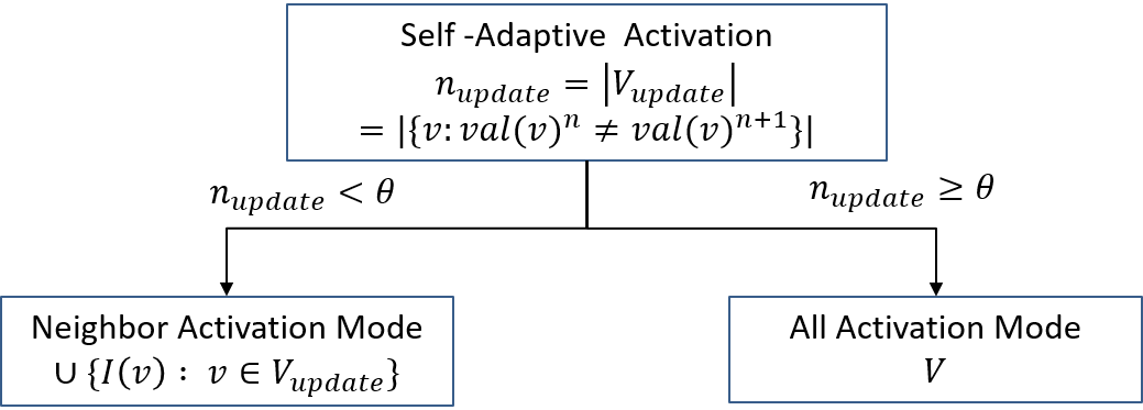
Figure 4: Self-Adaptive Activation.

Self-Adaptive Activation We also propose a self-adaptive activation mechanism to further improve vertex state maintenance efficiency based on the following observation.

We find that the above activation process works fine when not many vertices change values. However, when most vertices in a given graph update their values, more cost will be spent on obtaining and scanning inverted neighbor indices. For example, if $v_{2}$ and $v_{4}$ in Figure 3 update their values in iteration $n$, then all indices of $v_{2}$, $v^{\prime}_{2}$, $v_{4}$, and $v^{\prime}_{4}$ need to be obtained to know which vertices to activate in iteration $n+1$. In fact, all vertices will be activated in iteration $n+1$ because the union of these index sets equals to $V$. However, if we directly activate all vertices in $G$, the time to scan the dual neighbor indices can be saved.

Thus, instead of obtaining dual neighbor indices and scanning them in every iteration, we design two activation modes named $neighbor$ $activation$ $mode$ and $all$ $activation$ $mode$ for $\mathsf{Graph3S}$ and the system automatically chooses one of them for activation to get a better performance. The process of self-adaptive activation is illustrated in Figure 4. $V_{update}=\{v:val(v)^{n}\neq val(v)^{n+1}\}$ represents the vertices whose values change in current iteration. The total number of updated vertices $n\_change=|V_{update}|$ is recorded during computation in each iteration for the system to adaptively choose an activation mode. If $n\_change$ is smaller than a given threshold $\theta$ which means that few vertices change their values, then there is a low probability that the need-to-be-activated vertex set would approximate $V$. In this case, neighbor activation mode is chosen. Each updated vertex obtains its inverted neighbor index and activates the indexed vertices in $\cup\{I(v):v\in V_{update}\}$. Otherwise, all activation mode is chosen and all vertices in $V$ are directly activated in the next iteration. In this case, the scanning time of inverted neighbor indices are saved. Consider running $\mathsf{BFS}$ on $\mathsf{Graph3S}$. At earlier stage of execution, few vertices change value so neighbor activation mode is chosen. In the middle age, all activation mode is used because most vertices update their values. At the later age, fewer and fewer vertex values change. So the mode goes back to neighbor activation again.

3.4 Scalable

As we introduced above, $\mathsf{TLNE}$ requires a vertex to save all its neighborhood information locally. A direct way to implement $\mathsf{Graph3S}$ would be saving both vertex and edge information in memory. However, this is impractical for big graphs. To counter for this, we adopt a semi-caching strategy to enhance the scalability of $\mathsf{Graph3S}$. More specifically, we keep the vertex values in memory but edge information on disk. This is suitable for $\mathsf{Graph3S}$ because of the following three reasons:

• Firstly, a vertex only communicates with its neighbors in $\mathsf{Graph3S}$. During vertex computation, the edge information on disk will only be scanned linearly to get all neighbor information. On the other hand, vertex values are usually accessed randomly and constantly. It is better to save more random and constant accessed information in memory.

• Secondly, edge information rarely changes in our setting but vertex values are updated frequently. Note that we leave distributed system on dynamic graphs for future work.

• Thirdly, edge information usually costs more space than vertex information. Given a graph with $n$ vertices, the edge saving cost could be $O(n^{2})$ while the vertex information only costs $O(n)$. It is practical to save vertex values in memory.

From the above, we can see that the semi-caching model is a good balancing strategy between system efficiency and scalability for $\mathsf{Graph3S}$. Note that the semi-streaming model adopted in $\mathsf{GraphD}$ saves both edge information and messages on disk which actually weakens system performance in two aspects. Firstly, message streaming on disk slows down the system efficiency because of more disk accesses involved. Secondly, more disk space are required especially for message intensive algorithms and thus can easily cause out of disk error for real large graphs. These two aspects are both validated in our experiments.

4 Performance Studies

Our experimental results are outlined herein.

Table 3: Characteristics of datasets

Dataset	$|V|$	$|E|$	$deg_{max}$	$deg_{avg}$
$\mathsf{DB}$	986,207	13,414,472	979	13.60
$\mathsf{OR}$	2,997,167	212,698,418	27,466	70.97
$\mathsf{UK}$	18,520,343	523,574,516	194,955	28.27
$\mathsf{TW}$	41,652,230	2,936,729,768	2,997,487	70.51
$\mathsf{FR}$	124,836,180	3,612,134,270	5,214	28.93
$\mathsf{CW}$	978,409,098	42,574,107,469	75,611,696	43.51

Datasets. We used 6 real-world datasets of different sizes obtained from LAW [18]. $\mathsf{DBLP}$ ($\mathsf{DB}$), $\mathsf{Orkut}$ ($\mathsf{OR}$), $\mathsf{Twitter}$ ($\mathsf{TW}$) and $\mathsf{Friendster}$ ($\mathsf{FR}$) are social network graphs. $\mathsf{UK}$ and $\mathsf{ClueWeb}$ ($\mathsf{CW}$) are webgraphs. Table 3 shows the dataset details. $|V|$ and $|E|$ represent the number of vertices and edges respectively. $deg_{max}$ and $deg_{avg}$ denote the maximum and average vertex degree in each dataset respectively.

Experimental settings. We ran our experiments on a cluster of 10 machines, each with one 3.0GHz Intel Xeon E3-1120 CPU (4 cores), 64GB DDR3 RAM and 610GB disk. Unless specified, we use 6 machines, each with 4 cores by default.

We compared our system $\mathsf{Graph3S}$ with the representative systems: vertex-centric $\mathsf{Pregel}$, $\mathsf{Pregel+}$ [45] and $\mathsf{PowerGraph}$ [22], block-centric $\mathsf{Blogel}$ [42] and out-of-core system $\mathsf{GraphD}$ [46]. All systems are implemented in C++. We use $\theta=n/50$ as the threshold for self-adaptive activation in $\mathsf{Graph3S}$ because it guarantees a good system performance in most cases of our experiments. We use Yan’s implentation [45] of $\mathsf{Pregel}$. In terms of $\mathsf{Pregel+}$, we adopt the mirroring mode in the experiments. Similar to [45], we selected the vertex mirror threshold as the minimum value between 1000 and the value computed using their cost model. If not stated, we use the default settings of compared systems. For ease of expression, we represent the systems $\mathsf{Graph3S}$, $\mathsf{Pregel}$, $\mathsf{Pregel+}$, $\mathsf{PowerGraph}$, $\mathsf{Blogel}$ and $\mathsf{GraphD}$ by $\mathsf{G3S}$, $\mathsf{PRG}$, $\mathsf{PPL}$, $\mathsf{PG}$, $\mathsf{BLG}$ and $\mathsf{GD}$ respectively in the results. We also include results of $\mathsf{GraphD}$ with ID recoding technique represented by $\mathsf{GDIR}$ in the experiments.

Algorithms. To evaluate the system performances, we use 9 algorithms including single-phase algorithms: Breadth First Search ($\mathsf{BFS}$), Connected Component ($\mathsf{CC}$), Pagerank ($\mathsf{PR}$), Personalized Pagerank ($\mathsf{PPR}$), K-Core Decomposition ($\mathsf{Core}$) [25] and Graph Coloring ($\mathsf{Color}$) [19] and multi-phase algorithms: Maximal Independent Set ($\mathsf{MIS}$) [23], Maximal Matching ($\mathsf{MM}$) [19] and Triangle Counting ($\mathsf{TC}$). Among them, $\mathsf{BFS}$, $\mathsf{CC}$, $\mathsf{PR}$, $\mathsf{PPR}$ and $\mathsf{MIS}$ are separable algorithms. $\mathsf{Core}$, $\mathsf{Color}$ and $\mathsf{MM}$ are non-separable algorithms. An algorithm is separable if commutative and associative operation is to be applied on transmitted messages where optimization techniques like combiner can be applied. The ID recoding of $\mathsf{GraphD}$ is also only applicable to separable algorithms. Details of algorithm implementations are introduced as follows:

$\mathsf{BFS}$. We implemented $\mathsf{BFS}$ based on $\mathsf{SSSP}$ codes from authors of $\mathsf{PPL}$, $\mathsf{PG}$, $\mathsf{BLG}$ and $\mathsf{GraphD}$.

$\mathsf{CC}$. We directly use implementations of $\mathsf{CC}$ from authors of compared systems.

$\mathsf{PR}$, $\mathsf{PPR}$. We modified authors’ code of $\mathsf{PR}$ from $\mathsf{PPL}$, $\mathsf{PG}$ and $\mathsf{GraphD}$ by changing the termination condition to $\mathsf{10}$ iterations execution. For $\mathsf{Blogel}$, we used the authors’ implementation of $\mathsf{PR}$ and modified the termination condition of second step which operates in V-mode to $\mathsf{10}$ iterations computation. We implemented $\mathsf{PPR}$ based on $\mathsf{PR}$ for all systems.

$\mathsf{Color}$. We implemented $\mathsf{Color}$ for both $\mathsf{Pregel}$ and $\mathsf{Pregel+}$. An aggregator is designed to get the number of uncolored vertices and the program terminates when all vertices are colored. No combiner is used since a vertex needs to know the color value of each neighbor and the messages can’t be combined. $\mathsf{Color}$ is not implemented on $\mathsf{Blogel}$ because it is non-seperable where the advantage of block model could not be applied. For seperable computing like $\mathsf{BFS}$ and $\mathsf{CC}$, the value of a vertex could be updated continually inside a block. While the color value of a vertex is dependent on all other neighbors’ values which means it can’t be updated until the next iteration. It follows that $\mathsf{Blogel}$ needs the same number of iterations as a vertex-centric program and extra time on constructing and maintaining block information. We implemented $\mathsf{Color}$ on $\mathsf{PG}$ and $\mathsf{GD}$. ID recoding of $\mathsf{GDIR}$ is not applicable because $\mathsf{Color}$ is non-seperable.

$\mathsf{Core}$. Similar to $\mathsf{Color}$, we implemented $\mathsf{Core}$ for both $\mathsf{PRG}$ and $\mathsf{PPL}$ with no combiner. An aggregator is implemented to get the number of vertices whose core values are updated in a current iteration. The algorithm terminates when no core value changes. We also implemented $\mathsf{Core}$ on $\mathsf{PowerGraph}$. $\mathsf{Core}$ is not implemented on $\mathsf{Blogel}$ as computing core value of a vertex is non-seperable. $\mathsf{Core}$ is not implemented on $\mathsf{GD}$ and $\mathsf{GDIR}$ since aggregator is not provided on $\mathsf{GraphD}$ and termination condition cannot be implemented.

$\mathsf{TC}$. We implemented $\mathsf{TC}$ for for both $\mathsf{PRG}$ and $\mathsf{PPL}$. We adopted authors’ implementations of Triangle Counting for $\mathsf{PG}$ and $\mathsf{GD}$. ID recoding of $\mathsf{GDIR}$ is not applicable because $\mathsf{TC}$ is non-seperable. $\mathsf{TC}$ is not implemented on $\mathsf{Blogel}$ because it is non-seperable.

$\mathsf{MIS}$. We programmed $\mathsf{MIS}$ on $\mathsf{PRG}$, $\mathsf{PPL}$ and $\mathsf{PG}$. For $\mathsf{PRG}$ and $\mathsf{PG}$, a combiner is designed to combine messages. $\mathsf{MIS}$ is not implemented on $\mathsf{Blogel}$ because the block technique is not effective on multi-phase algorithms. $\mathsf{MIS}$ is also implemented on both $\mathsf{GD}$ and $\mathsf{GDIR}$.

$\mathsf{MM}$. We implemented $\mathsf{MM}$ for for both $\mathsf{PRG}$, $\mathsf{PPL}$ and $\mathsf{PowerGraph}$. Note that combiner is not applicable for $\mathsf{MM}$. We also implemented $\mathsf{MM}$ on $\mathsf{PowerGraph}$. Similar to $\mathsf{MIS}$, $\mathsf{MM}$ is not implemented on $\mathsf{Blogel}$. $\mathsf{GraphD}$ doesnot support $\mathsf{MM}$.

Metrics. We report the running time and communication cost to compare the system performances. Running time is counted from the moment when the data graph is totally loaded in the cluster to the time when the computation is completed. Note that data loading and result dumping time are excluded. Communication cost is the sum of data size transferred among workers in the cluster. Note that neither the cost of partitioning an input graph nor distributing it to workers is included.

Table 4: Number of Code Lines

System	$\mathsf{BFS}$	$\mathsf{PR}$	$\mathsf{CC}$	$\mathsf{Color}$	$\mathsf{Core}$	$\mathsf{TC}$	$\mathsf{MIS}$	$\mathsf{MM}$
$\mathsf{G3S}$	15	15	15	27	18	24	26	28
$\mathsf{PRG}$	101	107	95	131	122	120	112	116
$\mathsf{PPL}$	85	110	76	126	129	108	98	144
$\mathsf{PG}$	106	103		129	102	319	116	144
$\mathsf{BLG}$	221	328+178	16	NA	NA	NA	NA	NA
$\mathsf{GD}$	84	66	78	123	NA	108+57	97	NA
$\mathsf{GDIR}$	62	50	62	NA	NA	NA	78	NA

4.1 Usage Simplicity Comparison

Besides the discussion about the APIs comparison in Section 3.2.2, we also show the number of code lines in Table 4 using tokei [40] as a reference for simplicity comparison. From Table 4, we can see that implementations on $\mathsf{Graph3S}$ are much simpler compared with existing systems. This is easy to understand because the main task for a $\mathsf{Graph3S}$ user is to give a neighborhood expression for vertex computation. While the existing system users need to implement different APIs in terms of not only computation, but also tasks including communication, vertex state management, and so on. The difference is more severe when developing and tuning multi-phase algorithms like $\mathsf{TC}$, $\mathsf{MM}$ and $\mathsf{MIS}$ because the extra tasks in each phase accumulates for users to take.

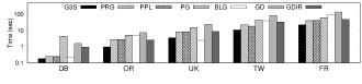
(a) $\mathsf{BFS}$

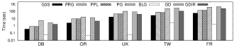
(b) $\mathsf{CC}$

(c) $\mathsf{PR}$

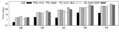
(d) $\mathsf{PPR}$

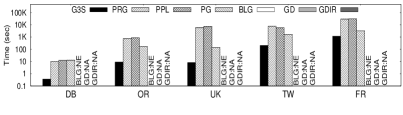
(e) $\mathsf{Core}$

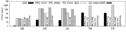
(f) $\mathsf{Color}$

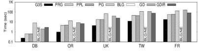
(g) $\mathsf{MIS}$

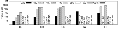
(h) $\mathsf{MM}$

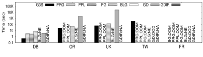
(i) $\mathsf{TC}$

Figure 5: Comparison with Existing Systems (Running Time)

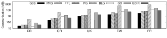
(a) $\mathsf{BFS}$

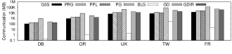
(b) $\mathsf{CC}$

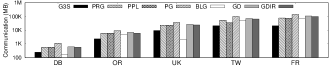
(c) $\mathsf{PR}$

(d) $\mathsf{PPR}$

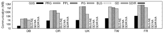
(e) $\mathsf{Core}$

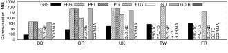
(f) $\mathsf{Color}$

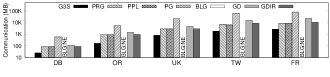
(g) $\mathsf{MIS}$

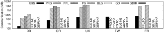
(h) $\mathsf{MM}$

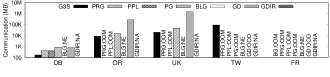
(i) $\mathsf{TC}$

Figure 6: Comparison with Existing Systems (Communication Cost)

4.2 Efficiency over Different Algorithms

We compared the system efficiency when running different algorithms over given datasets. The running time results are shown in Figure 5. We use NE and NA to represent Not Effective and Not Applicable cases as mentioned above respectively. OOM, OOD and TO represent Out Of Memory, Out Of Disk and Time Out respectively. We consider an algorithm running as time out when it can’t finish within 24 hours.

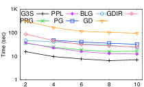
(a) $\mathsf{BFS}$ ($\mathsf{TW}$)

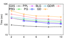
(b) $\mathsf{PR}$ ($\mathsf{TW}$)

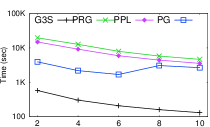
(c) $\mathsf{Core}$ ($\mathsf{TW}$)

(d) $\mathsf{MM}$ ($\mathsf{TW}$)

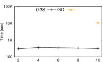
(e) $\mathsf{TC}$ ($\mathsf{TW}$)

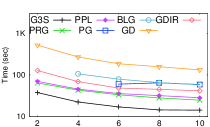
(f) $\mathsf{BFS}$ ($\mathsf{FR}$)

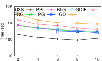
(g) $\mathsf{PR}$ ($\mathsf{FR}$)

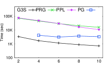
(h) $\mathsf{Core}$ ($\mathsf{FR}$)

(i) $\mathsf{MM}$ ($\mathsf{FR}$)

Figure 7: Scalability Test (Varying #machines)

From the results, we can see that, except for $\mathsf{CC}$ on $\mathsf{BLG}$, $\mathsf{Graph3S}$ outperforms all compared systems. For separable algorithms including $\mathsf{BFS}$, $\mathsf{CC}$, $\mathsf{PR}$, $\mathsf{PPR}$ and $\mathsf{MIS}$, $\mathsf{Graph3S}$ outperforms $\mathsf{PRG}$, $\mathsf{PPL}$, $\mathsf{PG}$, $\mathsf{BLG}$, $\mathsf{GD}$ and $\mathsf{GDIR}$ by 5.2x, 5.3x, 9.8x, 4.1x, 14.7x and 7.8x on average respectively. These algorithms are commonly used for system performance evaluations in existing works. $\mathsf{Graph3S}$ shows good speedup results. This proves the effectiveness of our speedy techniques as proposed in Section 3.3. Without the trouble of considering and designing combiners as with existing systems, the critical attributes, dual neighbor index and self-adaptive activation of $\mathsf{Graph3S}$ are able to guarantee a strong performance by saving computation and communication cost. For non-separable algorithms including $\mathsf{Core}$, $\mathsf{Color}$, $\mathsf{TC}$ and $\mathsf{MM}$, many optimizations in existing works like combiners, ID recoding are not applicable. Thus the outperformance of $\mathsf{Graph3S}$ is more severe in these cases. For example, $\mathsf{Graph3S}$ outperforms $\mathsf{PRG}$, $\mathsf{PPL}$, $\mathsf{PG}$, and $\mathsf{GD}$ by 198.2x, 249.3x, 89.4x, and 311.8x on average respectively. The speedup can even reach 906.0x when running $\mathsf{Core}$ on $\mathsf{UK}$ compared to $\mathsf{PPL}$. Note that the cases that systems can’t finish running algorithms are not included. These results demonstrate the consistent outperformance of our system over diverse algorithms. Among existing systems, vertex-centric systems have similar performances. But for separable algorithms like $\mathsf{BFS}$, $\mathsf{CC}$ and $\mathsf{MIS}$, $\mathsf{PRG}$ and $\mathsf{PPL}$ performs better than $\mathsf{PG}$ because of the combiner used effectively saves communication cost. One exception is $\mathsf{PR}$ and $\mathsf{PPR}$ because $\mathsf{PG}$ adopts delta caching. For non-separable algorithms like $\mathsf{Core}$, $\mathsf{Color}$ and $\mathsf{MM}$, a combiner is inapplicable leaving the superiority of $\mathsf{PRG}$ and $\mathsf{PPL}$ lacking. In terms of $\mathsf{PRG}$ and $\mathsf{PPL}$, although $\mathsf{PPL}$ has a mirroring technique, it cannot always beat $\mathsf{Pregel}$. This is because the cost saved by the mirroring technique does not always compensate for the additional cost of transferring mirror node messages. Another problem with $\mathsf{PPL}$ is that the mirror threshold needs to be designated by users which makes it difficult to achieve best system performance. This requires a user to be familiar with the system, algorithm and used dataset. A lower threshold will cause higher communication costs and memory consumption. At a certain point, it may cause OOM failure. This is why the authors recommend the threshold be at least 100 for large graphs. However, a too large threshold reduces the cost saving by mirroring technique. In fact, even the cost model given in their paper does not guarantee the best performance. The block-centric system $\mathsf{BLG}$ performs best among all compared systems running $\mathsf{CC}$. This is because the pre-processing partition of $\mathsf{BLG}$ already partitions connected subgraphs into the same machine. It favors the algorithm running within connected subgraphs because the vertices inside a block can keep computing until no more updates apply. In this way, the total number of algorithm supersteps is reduced. The performance of $\mathsf{GD}$ and $\mathsf{GDIR}$ are consistent with results from [47]. The results also show the effectiveness of IR recoding technique on separable algorithms. Generally, $\mathsf{GraphD}$ can’t beat in-memory vertex-centric systems. This is because it focuses on system scalability and is involved with disk accesses. Its better performance will be shown in the following scalability tests.

Communication Cost Comparison We also report the communication cost comparison results of evaluated systems in Figure 6. The results are mostly consistent with the running time presented above. More communication cost leads to longer running time. In most cases, $\mathsf{Graph3S}$ generates the least communication. This benefits from our critical attributes design which saves unnecessary attributes transformation cost. $\mathsf{PRG}$ and $\mathsf{PPL}$ have similar communication costs. $\mathsf{PG}$ incurs the highest communication cost in most tests. This is because other systems have different techniques to reduce communication cost, like combiner design and mirroring technique. $\mathsf{BLG}$ has less communication cost in $\mathsf{PR}$ and $\mathsf{PPR}$ because we only report the communication cost of B-mode (same with running time). The whole program needs to run V-mode first. Without ID recoding, $\mathsf{GD}$ has more communication cost than $\mathsf{GDIR}$ and $\mathsf{GDIR}$ generates similar cost with $\mathsf{PRG}$ and $\mathsf{PPL}$.

4.3 Scalability Test

In this section, we evaluate the scalability of all systems by varying the number of tested graph size and used machines respectively. Due to the space limit, we choose representative algorithms $\mathsf{BFS}$, $\mathsf{PR}$, $\mathsf{Core}$, $\mathsf{MM}$ and $\mathsf{TC}$ to report the results in this part.

Varying the Number of Machines. Firstly, we test the scalability of $\mathsf{Graph3S}$ in comparison with existing systems by varying the number of machines. For each machine, all four cores are used. We run selected algorithms over two large datasets $\mathsf{Twitter}$ and $\mathsf{Friendster}$. The results are shown in Figure 7. Note that the result of running $\mathsf{TC}$ on $\mathsf{Friendster}$ is not shown because only $\mathsf{GD}$ manages to finish when 10 machines are used within 24 hours (3800.24s).

The experimental results show that, in most cases, with the increasing number of machines used, better efficiencies are achieved. This is because the greater number of machines used, more parallel computation happens and the less computation time consumes. As a result, total running time reduces. However, more machines also means more communication cost. So, when saved computation cost doesn’t compensate increased communication cost, the total time couldn’t be reduced but will increase. This explains in some cases how the more machines used, more time is consumed. For example, running $\mathsf{Core}$ on $\mathsf{PG}$ over $\mathsf{Twitter}$, the total time increases when eight machines used compared to six machines.

We also find that the existing systems have different favourable algorithms. For example, in-memory systems show better performance running cpu-intensive algorithms like $\mathsf{BFS}$, $\mathsf{PR}$ and $\mathsf{Core}$. While out-of-core system $\mathsf{GraphD}$ shows poor efficiency performance. For example, it can’t finish in 24 hours running $\mathsf{Core}$ on either $\mathsf{Twitter}$ or $\mathsf{Friendster}$. This is understandable because $\mathsf{GraphD}$ uses disk to increase system scalability which meanwhile increases both computation and communication costs. However, for memory-intensive algorithms like $\mathsf{TC}$, disk-based system $\mathsf{GraphD}$ shows better performance than in-memory systems that usually run out of memory. For example, $\mathsf{GraphD}$ is the only system that finishes running $\mathsf{TC}$ on $\mathsf{Friendster}$.

Different from existing systems, $\mathsf{Graph3S}$ shows excellent overall performance for all kinds of algorithms. In terms of cpu-intensive algorithms, it outperforms existing in-memory systems. For example, it is averagely 36.6, 27.1 and 11.4 times faster than $\mathsf{PRG}$, $\mathsf{PPL}$ and $\mathsf{PG}$ respectively running $\mathsf{Core}$ on $\mathsf{Twitter}$ for different number of machines. For memory-intensive algorithms, $\mathsf{Graph3S}$ is competitive compared to $\mathsf{GD}$. For instance, $\mathsf{Graph3S}$ and $\mathsf{GD}$ are the only two systems that finish running $\mathsf{TC}$ on $\mathsf{Twitter}$. It is worth noticing that $\mathsf{GD}$ can only finish when all ten machines are used. Nevertheless, $\mathsf{Graph3S}$ is able to finish even when only two machines are used. Adding to this, though both systems finish when all 10 machines are used, $\mathsf{Graph3S}$ is 33.1 times faster than $\mathsf{GD}$. This further demonstrates the good combinational performance of $\mathsf{Graph3S}$ compared with existing systems.

(a) $\mathsf{BFS}$

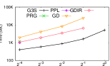
(b) $\mathsf{PR}$

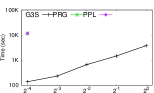
(c) $\mathsf{Core}$

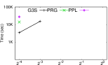
(d) $\mathsf{MM}$

Figure 8: Scalability Test (Varying #edges)

Varying Graph Size. We also test the system scalability by varying graph size. We adopt the largest used dataset $\mathsf{ClueWeb}$ and sample $2^{-1}$, $2^{-2}$, $2^{-3}$, $2^{-4}$ of all edges to vary the graph size. The experimental results are shown in Figure 8. Note that $\mathsf{TC}$ results are not reported because no system can finish running $\mathsf{TC}$ on any used dataset within 24 hours. Also, $\mathsf{PG}$ and $\mathsf{BLG}$ are not shown because they both couldn’t finish on used big graphs.

The results show that with dataset size increasing, the running time of all systems increases as well. All systems show similar increasing behavior. The results are consistent with that in Section 4.2. Our new system $\mathsf{Graph3S}$ shows superb scalability performance. $\mathsf{PRG}$ and $\mathsf{PPL}$ show good efficiency but can’t finish when the graph is too large. Disk-based system $\mathsf{GraphD}$ shows good scalability but is weak in efficiency. Especially for non-separable algorithms where ID recoding ($\mathsf{GDIR}$) is inapplicable, $\mathsf{GD}$ is very time-consuming. For example, when all edges in $\mathsf{ClueWeb}$ are used in $\mathsf{PR}$, $\mathsf{Graph3S}$ is the only system that can finish within 24 hours.

4.4 Other Issues

Fault tolerance is important to a system. It is not considered in current work because the authors of $\mathsf{PowerGraph}$ state in their paper [12] that the overhead, typically a few seconds for largest graph used, is relatively small compared to the total running time. This is consistent with our experiments. For example, the total time of $\mathsf{PG}$ for running $\mathsf{Color}$ on $\mathsf{Twitter}$, a dataset also used in their paper, is 23 hours. However, we leave the implementation of $\mathsf{Graph3S}$’s fault tolerance in the future. Also, asynchronous mode is not considered because it is not general and is only effective on algorithms with asymmetric convergence behavior and low workload [41].

5 Conclusion

The main goal of this paper was to develop a system for a good combinational performance of all simplicity, efficiency and scalability. We provide an idea of achiveing the goal by trading vertex comuunication flexibility. A simple, speedy and scalable $\mathsf{Graph3S}$ is designed with a simple programming model and different optimization techniques guaranteeing its efficiency and scalability. Extensive experimental results demonstrate the outstanding performance of $\mathsf{Graph3S}$ compared to existing systems. In the future, we aim to improve $\mathsf{Graph3S}$ by integrating general system optimization techniques and expand its application areas to support more algorithm categories like machine learning algorithms and more graph types like dynamic graphs and temporal analytics.

6 Acknowledgments

Lu Qin is supported by ARC DE140100999 and DP160101513. Lijun Chang is supported by ARC DP160101513 and FT180100256. Ying Zhang is supported by ARC DE140100679 and DP170103710. Xuemin Lin is supported by NSFC61232006, ARC DP150102728, DP140103578 and DP170101628.

References

- [1] Y. Bu, V. Borkar, J. Jia, M. J. Carey, and T. Condie. Pregelix: Big (ger) graph analytics on a dataflow engine. Proceedings of the VLDB Endowment, 8(2):161–172, 2014.
- [2] Y. Bu, B. Howe, M. Balazinska, and M. D. Ernst. Haloop: efficient iterative data processing on large clusters. Proceedings of the VLDB Endowment, 3(1-2):285–296, 2010.
- [3] Q. Cai, W. Guo, H. Zhang, D. Agrawal, G. Chen, B. C. Ooi, K.-L. Tan, Y. M. Teo, and S. Wang. Efficient distributed memory management with rdma and caching. Proceedings of the VLDB Endowment, 11(11):1604–1617, 2018.
- [4] H. Chen, M. Liu, Y. Zhao, X. Yan, D. Yan, and J. Cheng. G-miner: an efficient task-oriented graph mining system. In Proceedings of the Thirteenth EuroSys Conference, page 32. ACM, 2018.
- [5] J. Cheng, Q. Liu, Z. Li, W. Fan, J. C. Lui, and C. He. Venus: Vertex-centric streamlined graph computation on a single pc. In Data Engineering (ICDE), 2015 IEEE 31st International Conference on, pages 1131–1142. IEEE, 2015.
- [6] Y. Chi, G. Dai, Y. Wang, G. Sun, G. Li, and H. Yang. Nxgraph: An efficient graph processing system on a single machine. In Data Engineering (ICDE), 2016 IEEE 32nd International Conference on, pages 409–420. IEEE, 2016.
- [7] D. M. Da Zheng, R. Burns, J. Vogelstein, C. E. Priebe, and A. S. Szalay. Flashgraph: Processing billion-node graphs on an array of commodity ssds. In Proceedings of the 13th USENIX Conference on File and Storage Technologies, pages 45–58, 2015.
- [8] R. Dathathri, G. Gill, L. Hoang, H.-V. Dang, A. Brooks, N. Dryden, M. Snir, and K. Pingali. Gluon: A communication-optimizing substrate for distributed heterogeneous graph analytics. In Proceedings of the 39th ACM SIGPLAN Conference on Programming Language Design and Implementation, pages 752–768. ACM, 2018.
- [9] J. Dean and S. Ghemawat. Mapreduce: simplified data processing on large clusters. Communications of the ACM, 51(1):107–113, 2008.
- [10] W. Fan, J. Xu, Y. Wu, W. Yu, J. Jiang, Z. Zheng, B. Zhang, Y. Cao, and C. Tian. Parallelizing sequential graph computations. In Proceedings of the 2017 ACM International Conference on Management of Data, pages 495–510. ACM, 2017.
- [11] giraph.apache.org. Giraph, 2011.
- [12] J. E. Gonzalez, Y. Low, H. Gu, D. Bickson, and C. Guestrin. Powergraph: Distributed graph-parallel computation on natural graphs. In Presented as part of the 10th USENIX Symposium on Operating Systems Design and Implementation (OSDI 12), pages 17–30, 2012.
- [13] M. Han and K. Daudjee. Giraph unchained: Barrierless asynchronous parallel execution in pregel-like graph processing systems. Proceedings of the VLDB Endowment, 8(9):950–961, 2015.
- [14] W.-S. Han, S. Lee, K. Park, J.-H. Lee, M.-S. Kim, J. Kim, and H. Yu. Turbograph: a fast parallel graph engine handling billion-scale graphs in a single pc. In Proceedings of the 19th ACM SIGKDD international conference on Knowledge discovery and data mining, pages 77–85. ACM, 2013.
- [15] V. Kalavri, V. Vlassov, and S. Haridi. High-level programming abstractions for distributed graph processing. IEEE Transactions on Knowledge and Data Engineering, 30(2):305–324, 2017.
- [16] S. Ko and W.-S. Han. Turbograph++: A scalable and fast graph analytics system. In Proceedings of the 2018 International Conference on Management of Data, pages 395–410. ACM, 2018.
- [17] A. Kyrola, G. E. Blelloch, and C. Guestrin. Graphchi: Large-scale graph computation on just a pc. USENIX, 2012.
- [18] law.di.unimi.it. The laboratory for web algorithmics, 2002.
- [19] N. Linial. Locality in distributed graph algorithms. SIAM Journal on Computing, 21(1):193–201, 1992.
- [20] H. Liu and H. H. Huang. Graphene: Fine-grained io management for graph computing. In Proceedings of the 15th Usenix Conference on File and Storage Technologies, FAST’17, pages 285–299, Berkeley, CA, USA, 2017. USENIX Association.
- [21] Y. Low, D. Bickson, J. Gonzalez, C. Guestrin, A. Kyrola, and J. M. Hellerstein. Distributed graphlab: a framework for machine learning and data mining in the cloud. Proceedings of the VLDB Endowment, 5(8):716–727, 2012.
- [22] Y. Low, J. Gonzalez, A. Kyrola, D. Bickson, C. Guestrin, and J. M. Hellerstein. Powergraph, 2010.
- [23] M. Luby. A simple parallel algorithm for the maximal independent set problem. SIAM journal on computing, 15(4):1036–1053, 1986.
- [24] G. Malewicz, M. H. Austern, A. J. Bik, J. C. Dehnert, I. Horn, N. Leiser, and G. Czajkowski. Pregel: a system for large-scale graph processing. In Proceedings of the 2010 ACM SIGMOD International Conference on Management of data, pages 135–146. ACM, 2010.
- [25] A. Montresor, F. De Pellegrini, and D. Miorandi. Distributed k-core decomposition. IEEE Transactions on parallel and distributed systems, 24(2):288–300, 2012.
- [26] D. Nguyen, A. Lenharth, and K. Pingali. A lightweight infrastructure for graph analytics. In Proceedings of the Twenty-Fourth ACM Symposium on Operating Systems Principles, pages 456–471. ACM, 2013.
- [27] A. Quamar, A. Deshpande, and J. Lin. Nscale: neighborhood-centric large-scale graph analytics in the cloud. The VLDB Journal—The International Journal on Very Large Data Bases, 25(2):125–150, 2016.
- [28] A. Roy, I. Mihailovic, and W. Zwaenepoel. X-stream: Edge-centric graph processing using streaming partitions. In Proceedings of the Twenty-Fourth ACM Symposium on Operating Systems Principles, pages 472–488. ACM, 2013.
- [29] S. Salihoglu and J. Widom. Gps: a graph processing system. In Proceedings of the 25th International Conference on Scientific and Statistical Database Management, page 22. ACM, 2013.
- [30] S. Salihoglu and J. Widom. Optimizing graph algorithms on pregel-like systems. Proceedings of the VLDB Endowment, 7(7):577–588, 2014.
- [31] J. Shun and G. E. Blelloch. Ligra: a lightweight graph processing framework for shared memory. In ACM Sigplan Notices, volume 48, pages 135–146. ACM, 2013.
- [32] S. Song, X. Liu, Q. Wu, A. Gerstlauer, T. Li, and L. K. John. Start late or finish early: A distributed graph processing system with redundancy reduction. PVLDB, 12(2):154–168, 2018.
- [33] C. H. Teixeira, A. J. Fonseca, M. Serafini, G. Siganos, M. J. Zaki, and A. Aboulnaga. Arabesque: a system for distributed graph mining. In Proceedings of the 25th Symposium on Operating Systems Principles, pages 425–440. ACM, 2015.
- [34] Y. Tian, A. Balmin, S. A. Corsten, S. Tatikonda, and J. McPherson. From think like a vertex to think like a graph. Proceedings of the VLDB Endowment, 7(3):193–204, 2013.
- [35] L. G. Valiant. A bridging model for parallel computation. Communications of the ACM, 33(8):103–111, 1990.
- [36] K. Vora, G. H. Xu, and R. Gupta. Load the edges you need: A generic i/o optimization for disk-based graph processing. In USENIX Annual Technical Conference, pages 507–522, 2016.
- [37] G. Wang, W. Xie, A. J. Demers, and J. Gehrke. Asynchronous large-scale graph processing made easy. In CIDR, volume 13, pages 3–6, 2013.
- [38] Z. Wang, Y. Gu, Y. Bao, G. Yu, and J. X. Yu. Hybrid pulling/pushing for i/o-efficient distributed and iterative graph computing. In Proceedings of the 2016 International Conference on Management of Data, pages 479–494. ACM, 2016.
- [39] wikipedia.org. Graph coloring - wikipedia.
- [40] XAMPPRocky and contributors. tokei, 2015.
- [41] D. Yan, Y. Bu, Y. Tian, A. Deshpande, et al. Big graph analytics platforms. Foundations and Trends® in Databases, 7(1-2):1–195, 2017.
- [42] D. Yan, J. Cheng, Y. Lu, and W. Ng. Blogel, 2014.
- [43] D. Yan, J. Cheng, Y. Lu, and W. Ng. Blogel: A block-centric framework for distributed computation on real-world graphs. Proceedings of the VLDB Endowment, 7(14):1981–1992, 2014.
- [44] D. Yan, J. Cheng, Y. Lu, and W. Ng. Effective techniques for message reduction and load balancing in distributed graph computation. In Proceedings of the 24th International Conference on World Wide Web, pages 1307–1317. International World Wide Web Conferences Steering Committee, 2015.
- [45] D. Yan, J. Cheng, Y. Lu, and W. Ng. Pregel+, 2015.
- [46] D. Yan, Y. Huang, M. Liu, H. Chen, J. Cheng, H. Wu, and C. Zhang. Graphd, 2018.
- [47] D. Yan, Y. Huang, M. Liu, H. Chen, J. Cheng, H. Wu, and C. Zhang. Graphd: distributed vertex-centric graph processing beyond the memory limit. IEEE Transactions on Parallel and Distributed Systems, 29(1):99–114, 2018.
- [48] P. Yuan, W. Zhang, C. Xie, H. Jin, L. Liu, and K. Lee. Fast iterative graph computation: A path centric approach. In Proceedings of the International Conference for High Performance Computing, Networking, Storage and Analysis, pages 401–412. IEEE Press, 2014.
- [49] Q. Zhang, A. Acharya, H. Chen, S. Arora, A. Chen, V. Liu, and B. T. Loo. Optimizing declarative graph queries at large scale. In Proceedings of the 2019 International Conference on Management of Data, pages 1411–1428. ACM, 2019.
- [50] J. Zhong and B. He. Medusa: Simplified graph processing on gpus. IEEE Transactions on Parallel and Distributed Systems, 25(6):1543–1552, 2014.
- [51] X. Zhu, W. Chen, W. Zheng, and X. Ma. Gemini: A computation-centric distributed graph processing system. In OSDI, pages 301–316, 2016.
- [52] X. Zhu, W. Han, and W. Chen. Gridgraph: Large-scale graph processing on a single machine using 2-level hierarchical partitioning. In USENIX Annual Technical Conference, pages 375–386, 2015.