Spatially resolved velocity structure in jets of DF Tau and UY Aur A

Abstract

Young stars accrete mass and angular momentum from their circumstellar disks. Some of them also drive outflows, which can be distinguished in optical forbidden emission lines (FELs). We analyze a sample of binary T Tauri stars observed with long-slit spectroscopy by the Hubble Space Telescope (HST), searching for spatially resolved outflows. We detect resolved [O i] emission in two cases out of twenty one. In DF Tau we resolve high and medium velocity outflows in a jet and counterjet out to 60 au. The outflows are accelerated within the inner 12 au and retain a constant speed thereafter. In UY Aur, we detect a blue- and a red-shifted outflow from UY Aur A, as well as a blue-shifted jet from UY Aur B. All of these features have been seen in [Fe ii] with data taken ten years apart indicating that the underlying outflow pattern is stable on these timescales.

1 Introduction

Star formation occurs when large clouds of gas and dust collapse due to gravity. The clouds are inhomogeneous in density and they fragment into smaller structures, where the center of each collapsing sub-cloud may become a star or system of stars. Very few of the resulting stars are massive and hot. By far the largest number will evolve into late-type stars with spectral types in the M-F range. Most stars are members of a binary or multiple multiple systems (see e.g. review by Duchêne et al., 2007). The infalling envelope flattens to a circumstellar disk, making the stars visible in the optical. Low-mass stars in this stage are called classical T Tauri stars (CTTS). For a few Myrs, planet formation can take place before the disk disperses. For binaries or higher-order multiple systems, the disk can belong to an individual star or surround a close binary pair depending on the mass and separation of the components.

Mass is accreted through these disks onto the stars. However, conservation of angular momentum demands that some mass is ejected and carries away the angular momentum accreted through the disk. Mass loss occurs through wide-angle disk winds, but in some systems we also see highly collimated jets (see Frank et al., 2014, for a review). Based on different theoretical ideas, models of stellar winds (Kwan & Tademaru, 1988; Matt & Pudritz, 2005), X-winds (Shu et al., 1994) and disk winds (Blandford & Payne, 1982; Anderson et al., 2005) have been proposed that can launch mass into an outflow. Ultimately these mass flows must be powered from the gravitational energy released in the accretion process. The collimation of the outflow into a jet is hard to explain without toroidal magnetic fields generated by magnetic field that is dragged inwards in the accretion process (see review by Lovelace et al., 2014). However, we do not know in detail how energy and momentum are converted from an inflow to an outflow (e.g. Matt et al., 2010, and references therein). Observationaly, we see that the outflow rate is roughly one tenth of the accretion rate (Cabrit et al., 1990; Coffey et al., 2008), supporting a causal relation between outflows and energy released in the accretion process.

Full 3D magneto-hydrodynamic simulations of jet launching are numerically challenging and early work has been limited to lower dimensions and/or ideal MHD (e.g. Casse & Keppens, 2002; Dyda et al., 2015). For binary stars, an added complication is the influence that one member of the binary has on the disk and outflow from the other star. The most important parameter to determine the strength of any gravitational torque is the binary separation. Simulations for binaries separated by no more than 15 au or so indicate that no jets are launched for high disk-orbit inclinations. For moderate inclination, the jet axis can precess in a cone of a few degrees opening angle (Sheikhnezami & Fendt, 2018). We refer the reader to the introduction in Sheikhnezami & Fendt (2018) for a review of this topic. In contrast, in wide binaries, simulations and observations show random alignments between outflows from both members of the binary (Offner et al., 2016).

Forbidden optical emission lines (FELs) are a good way to find and study such jets, since the stellar photosphere and the accretion shock are too dense to contribute significantly to the emission. These jets typically have an onion-like structure with a fast component at the center surrounded by increasingly slower and less collimated components further out (Bacciotti et al., 2000).

If a jet is detected in several emission lines, line ratios can be used to calculate density and ionization fraction of emission components in the jet with typical jet densities in the range $10^{3}-10^{5}\;\mathrm{cm}^{-3}$ (e.g. Solf & Boehm, 1993; Bacciotti & Eislöffel, 1999; Lavalley-Fouquet et al., 2000; Schneider et al., 2013). In turn the density and the velocity give mass loss rates. Different outflow components show different velocities. For example, in the well-studied CTTS DG Tau Schneider et al. (2013) find [O i] in a low-velocity component (LVC, about 60 km s^-1) which can be detected as close as 15 au from the star and a medium-velocity component (MVC, about 130 km s^-1) first detected at about 50 au from the source. The MVC in DG Tau slows down at larger distances. FELs can be seen up to at least 600 au from the star in DG Tau (Solf & Boehm, 1993). FELs have also been detected in outflows from binaries, in some cases each star launches its own jet (e.g. in T Tau Solf & Böhm, 1999), in other systems it appears that the outflow is launched from a common circumbinary disk or at least that the individual jets from both components of the binary merge early (Mundt et al., 2010).

While a single spectrum is sufficient to detect the presence of a FEL, spatially resolved data is necessary to study how outflows accelerate and decelerate. In this work, we reanalyze archival data from the Hubble Space Telescope (HST) Program ID 7310 to search for FELs that are spatially resolved.

In section 2 we describe the observations and the data reduction. Section 3 presents our immediate results. We discuss the resolved emission from DF Tau and UY Aur in section 4 and end with a short summary in section 5.

2 Observations and data reduction

Table 1: Log of observations

OBSID G750L	OBSID G750M	Target	Observation Date	Aperture	Position angle (deg)
o55101010	o55101020	FO TAU	1999-10-17	52X0.2	50.15
o55102010	o55102020	DD TAU	1999-09-05	52X0.5	64.54
o55104010	o55104020	UZ TAU-W	1999-11-02	52X0.2	52.54
o55105010	o55105020	LKCA 7	1999-01-25	52X0.2	250.0
o55106010	o55106020	LKHA 332	1998-12-23	52X0.2	251.0
o55107010	o55107020	UY AUR	1998-12-25	52X0.2	271.0
o55108010	o55108020	040047+2603W	1998-12-04	52X0.2	272.0
o55109010	o55109020	FQ TAU	1998-12-05	52X0.5	303.0
o55110010	o55110020	FS TAU	2000-12-13	52X0.2	309.0
o55111010	o55111020	HARO6-28	1998-12-02	52X0.2	290.1
o55112010	o55112020	LKHA332G2	1998-12-12	52X0.5	269.4
o55113010	o55113020	040142+2150	1998-12-01	52X0.2	289.0
o55114010	o55114020	IS TAU	2000-12-03	52X0.2	317.0
o55115010	o55115020	FV TAU	2000-12-03	52X0.5	322.4
o55116010	o55116020	FV TAU-C	1998-12-02	52X0.2	337.0
o55117010	o55117020	GH TAU	2000-12-01	52X0.2	350.8
o55118010	o55118020	LKHA 331	1999-10-08	36X0.6P45	100.0
o55119010	o55119020	UZ TAU-W-OFF	2000-09-04	52X0.5	64.79
o55120010	o55120020	DF TAU	1998-11-26	52X0.2	18.04
o55121010	o55121020	XZ TAU	2000-12-02	52X0.2	194.1
o55122010	o55122020	V807 TAU	1998-11-30	52X0.2	19.03

Hubble Space Telescope (HST) Program ID 7310 targeted binary T Tauri stars with long-slit spectroscopy using the Space Telescope Imaging Spectrograph (STIS). The long slit is always oriented such that both components of the binary are observed. Hartigan & Kenyon (2003) analyze the spectra of both stellar components to determine stellar properties and accretion diagnostics. In this work, we aim to spatially resolve the emission in FELs along the slit.

Table 1 lists the observations presented in this paper. The observations for each of the stars were taken using two different gratings: G750L and G750M, with central wavelengths of 7751 Å and 6252 Å with exposure times of 360 s and 1080 s respectively. For each target system the observations were consecutive in the same orbit. Position angles are measured East of North. Hartigan & Kenyon (2003) lists properties (including binary separation and position angle, but also derived properties like stellar mass and accretion) in tables for all targets.

Our analysis begins from the pipeline reduced 2-dimensional sx2 files; these files have one spectral axis and one spatial axis for the coordinate along the slit. For each wavelength in sx2 we fit a single Gaussian to approximate the spatial flux distribution (dominated by the point-spread function (PSF) of the star), taking into account regions flagged for data quality by the pipeline. While this does not capture all features of the instrumental PSF, it describes the signal close to the peak of the emission well and allows a numerically stable fit of the position of the peak.

The measured peak position of the Gaussian changes with wavelength in a smooth manner, both due to minor misalignment between slit and CCD as well as due to the distortion corrections done in the data pipeline. The scatter in the fit results can be taken as an estimate of uncertainty of our fits. If both components of the binary system are within a few arcseconds of each other, a fit using two Gaussians is performed. All fits are visually inspected.

FELs are tracers of outflows because they can only be formed in low-density environments. We search for changes of the fitted position of the Gaussian, i.e. changes in the mean position of the emission caused by a resolved emission component offset from the central star around the wavelength of the FELs in table 2. Limiting our search in this way reduces the rate of false-positives.

Table 2: Lines searched for spatial extension

line	wavelength [Å]
[O I]	6302.0
[O I]	6365.5
[O III]	5008.240
[O III]	4960.295
[O III]	4364.436
[N II]	6549.86
[N II]	6585.27
[S II]	6718.29
[S II]	6732.67

To investigate resolved emission in more detail we subtract the contribution of the stellar continuum similar to the method of Schneider et al. (2013): For every row of in the image (in the dispersion direction) we select a region of interest centered on the position of the FEL (15 pixels wide for the G750M data and 2 pixels wide in the G750L data, where the FELS are not spectrally resolved). Assuming that the PSF is only slowly changing with wavelength and that the stellar emission around the FELs is continuum dominated, we fit a second degree polynomial to the data to the left and right of the FEL. The region used for the fit is 10 pixels wide in the G750M data and 5 pixels wide in the G750L data. We subtract the value of the polynomial for every row of data in the FEL region. The remaining images should display signatures of jets if there are any, and can be used to examine jet profiles and intensities.

3 Results

3.1 Significantly extended FELs

We detected significantly extended emission only in two out of 21 objects, DF Tau and UY Aur. In both cases, the extension is seen in the [O i] lines, but is not significantly detected in any other FEL. Hartigan & Kenyon (2003) already noted that the on-source [O i] line profile shows different kinematic components for both components of the DF Tau binary and for the primary of UY Aur, while all other targets have simple [O i] line profiles. Hartigan & Kenyon (2003) also discuss the FS Tau (catalog ) primary where they note an [O i] line that appears spatially extended. FS Tau shows an extension in our processing, however, this is due entirely to the signal from a single pixel, which is flagged by the data processing pipeline as having a high dark current rate. No spatial extension is seen after removing that spurious signal.

We show position-velocity-diagrams (PVD) for DF Tau in Fig. 1 and for UY Aur in Fig. 3. In the PVDs the origin of the spatial coordinate is set on the position of the primary star. Resolved FEL emission is seen as a bulge in the vicinity of the rest wavelength in the emission line. Where resolved FEL emission is seen, we quantify the peak velocity and width of the emission by fitting Gaussians to the spectrum at each position (row of data in the PVD). See Figure 2 for examples of those fits at different positions.

Table 3: Measured fluxes

source	velocity	FWHM	6300 Å	6363 Å	$\dot{M}$
	[km s-1]	[km s-1]
DF Tau	-150	40	3	1	14
DF Tau	-50	60	2	.4	3
DF Tau	+150	40	3	5	14
UY Aur A	-150	30	0.6	2	5
UY Aur A	+50	40	0.3	1	0.8

3.1.1 DF Tau

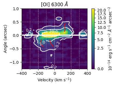
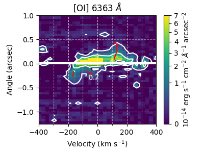
Figure 1: Position velocity diagrams (PVD) for DF Tau; the two components of the binary are not resolved and the stellar continuum emission has been subtracted (See text). The x-axis shows the velocity with respect to the feature rest wavelength in the velocity frame of the star and the y-axis is the distance along the slit. The continuum emission from the two stars has been subtracted. The color scale is chosen to highlight faint emission features; negative values or brighter fluxes are shown as purple or yellow, respectively. White lines shows the position of each star in the binary. Since the two components in DF Tau are unresolved, only one line is visible in this figure. Contours show flux densities in $10^{-14}$ erg s^-1 cm^-2 Å^-1 arcsec^-2. The red lines mark the position of the emission peak for jet components (see text for details).

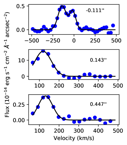
Figure 2: Examples of jet component fits for DF Tau for three different spatial positions. Data is continuum subtracted close to the 6300 Å line. Statistical errors are smaller than plot symbols, but the true uncertainty on eahc data point is dominated by systematics from the subtraction process. Each plot is labeled with the angular coordinate corresponding to that pixel row. The top plot corresponds to the blue-shifted component with the two Gaussians resolved. The middle plot corresponds to the red-shifted component close to the star, while the bottom plot corresponds to the faintest part of the red-shifted component. The Gaussian fit works well in all of these cases.

The [O i] position-velocity-diagram (PVD) for DF Tau is shown in figure 1 corrected for the stellar radial velocity from Gontcharov (2006). In order to trace how outflow components accelerate or decelerate with increasing distance from the source, we fit one or more Gaussian emission components to each row of data (each row represents a spectrum at a constant distance from the source). Red lines in the figure mark the velocities of the peak of the fitted Gaussians. Examples of these fits are shown in Fig 2. The statistical uncertainty from the fit is less than the line thickness. We sum the fluxes and average the $FWHM$ for all fitted Gaussians further than three pixels from the star center for each outflow component (table 3). Uncertainties on the fluxes are dominated by the subtraction procedure and can be estimated by comparing the fluxes seen in [O i] 6300Å and [O i] 6363Å lines, whose theoretical ratio should be 3 (Storey & Zeippen, 2000). Based on the observed ratios, fluxes are accurate to approximately 50%.

Both sides of the jet can be traced to a similar distance. The observed velocity of the high velocity component (HVC) of the approaching jet is about -150 to -200 km s^-1. Since we do not know the inclination angle with respect to the line-of-sight observed velocities are lower boundaries to the true jet speed. We also identify a medium velocity component (MVC) around -50 km s^-1, but the emission is weaker than the HVC. There is a red-shifted counter jet at a velocity around +150 km s^-1 and a single emission feature at 50 km s^-1, located about 0$\farcs$6 from the star (72 au projected on the plane of the sky). The HVC of jet and counterjet is seen to about 0$\farcs$5 (60 au). All those features are seen in both [O i] lines, which gives us confidence that even the weaker features are real detections and not just background fluctuations. We do not see significant changes in the velocity, thus all outflows must be accelerated in the inner 0$\farcs$1 (12 au) where we do not resolve the jet emission.

For a divergent flow with constant velocity, the divergence of the jet streamlines is related to the $FWHM$ for the observed FEL. Using the simplifying assumption of a homogeneously emitting cone, we can use eqn 5 from Mundt et al. (1990) and the values in our table 3. The inclination of the DF Tau outflow cannot be directly pole-on, since it is spatially resolved in our data. Assuming an inclination $>20$°, we derive outflow opening angles $<1$°for the fast components and $<3$°for the slower component. As discussed in Section 1, jets from CTTS are typically not homogeneous, but this nevertheless shows that we are observing highly collimated jets and not wide-angle outflows. Note that the measured values for the $FWHM$ are a convolution of the line profile of the FEL and the instrumental resolution and thus the true opening angles would be even smaller.

3.1.2 UY Aur

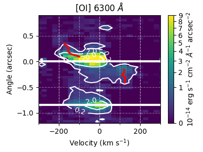
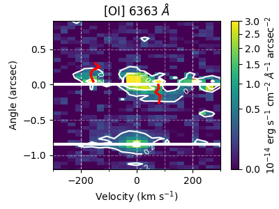
Figure 3: Position velocity diagrams for subtracted image of UY Aur. The stellar continuum emission has been subtracted for both members of the UY Aur binary (see text). The x-axis shows the velocity with respect to the feature rest wavelength in the velocity frame of the star UY Aur A and the y-axis the distance along the slit. The position of both components of the UY Aur AB binary are marked by white lines. The red lines mark the position of the emission peak for jet components (see text for details).

We use the radial velocities from Nguyen et al. (2012) for UY Aur and show a PVD in figure 3. Like in DF Tau, the position of the peak flux for resolved FEL emission is determined by fitting Gaussians to the spectrum at each position and the resulting statistical uncertainties are smaller than the width of the red line in the figure. There is a HVC around -150 to -200 km s^-1 visible to about 0$\farcs$25 (40 au).This outflow component seems to originate on the primary and move away from the secondary. There is a second component, also originating from the primary (the origin on the y-axis in the figure), that points towards the secondary with a velocity around +150 km s^-1. In [O i] 6366Å, the same components are seen but the signal is lower. Both plots in the figures also show apparent emission close to 0 km s^-1, but this is an artifact of our subtraction procedure. The emission is centered on the star. Since our procedure subtracts the stellar continuum only, the wings of the PSF of the [O i] emission at the stellar location remain in the images. Fluxes are given in table 3. We integrate only the resolved signal further than three pixels away from the star to account for that. The low $FWHM$ sets strict limits on the opening angle of the UY Aur outflow, showing that we observe highly collimated jets and not wide-angle outflows.

3.2 Upper limits

The [O i] lines are the only FELs from table 2 that fall in the wavelength range of the G750M grating with the available central wavelength settings. We attempt to detect other lines in the G750L data using our subtraction procedure but cannot perform this measurement for the [N ii] lines, because they are too close to the H$\alpha$ line. The [O i] lines are kinematically unresolved, but fluxes are consistent with what is seen in G750M gratings. We inspected figures analogous to figures 1 and 3 for several regions free of FELs to determine the average noise. We conclude that the [S ii] lines are not detected for any source from table 1. Line-free regions and the [S ii] lines show residuals that decline with distance from the stars with an average of $10^{-14}$ erg s^-1 Å^-1 arcsec^-2 at 0$\farcs$2 and 0.05$\times 10^{-14}$ erg s^-1 Å^-1 arcsec^-2 at 0$\farcs$5. Thus, we conclude that the [O i] lines are at least 3-5 times stronger than [S ii] in DF Tau and at least two times stronger in UY Aur. We also checked H$\alpha$ for extension, but did not find extended emission that could indicate a presence of a jet.

3.3 Mass loss rates

With some assumptions on the physical conditions in the jet, we can estimate the total mass loss rate in the resolved outflow components. Following Hartigan et al. (1994), we take a plasma with solar abundances emitting close to the peak formation temperature of the [O i] lines. Any jet components that are located outside the aperture, so hot that oxygen is ionized or so cool that that [O i] 6300Å is not excited, or with densities above the critical density for [O i] ($10^{6}$ cm^-3), are not accounted for in this estimate. Thus, the estimate is a lower limit in the total mass flux in the jet. We use

$$\dot{M} = 5.95\times 10^{-8}\left(\frac{n_{e}}{10^{3}\textnormal{ cm}^{-3}}\right)^{-1}\left(\frac{L_{6300}}{10^{-4}L_{\sun}}\right)$$ (1)

$$\times\left(\frac{v_{sky}}{100\textnormal{ km s}^{-1}}\right)\left(\frac{l_{sky}}{10^{16}\textnormal{ cm}}\right)^{-1}M_{\sun}\textnormal{ yr}^{-1}\ ,$$

which is eqn. 10 from Hartigan et al. (1994). Since no other FELS are detected, the density can only be constrained to be below the critical density for [O i]. For the following discussion, we will use $n_{e}=10^{3}$ cm^-3 as the fiducial density because this number was observed in the jet of DG Tau (Lavalley-Fouquet et al., 2000), a well-studied collimated outflow in the same star forming region, launched from a star of similar age and only slightly earlier spectral type (K6 vs M0-M2). Several FELs are observed in DG Tau, thus the density can be calculated from FEL ratios, unlike in our data from DF Tau and UY Aur. In practice, the density likely varies with distance to the source in all jets (as it does in the jet from DG Tau) and might also differ between DF Tau and UY Aur. All values for the outflow mass flux scale with $1/n_{e}$. Even if the density was known in some way (e.g. a future observation), the uncertainty in the remaining factors in the equation would still make the estimated mass loss uncertain by a factor of a few.

4 Discussion

We detect spatially extended emission in about 10% of observations. The two components of the DF Tau binary are the strongest accretors in the sample (Hartigan & Kenyon, 2003), while UY Aur is close to the median. If mass flux of the outflow is roughly proportional to the accretion rate as suggested by observations (Cabrit et al., 1990; Coffey et al., 2008), then we would not expect to detect outflows from any source with accretion weaker than UY Aur. There are six binaries in the sample with accretion rates between UY Aur and DF Tau, where a jet could be detected, if it scales with the accretion rate and happens to be roughly aligned with the slit in the observations. Assuming that we can detect spatially resolved emission for jets misaligend with the slit up to about 30 degrees, actually detecting jets in three out of 16 stars (eight binaries) with mass accretion rates of UY Aur or higher, is statistically consistent with all stars having jet emission in a random orientation. However, the fact that the twobinaries where extended emission is seen are the same binaries where at least one component shows multiple kinematic components in the [O i] emission lines (Hartigan & Kenyon, 2003) suggests that the other objects may not have as pronounced outflows.

We compare our detections to other observations of the same jets in the literature to put the properties of these jets into context.

4.1 DF Tau

DF Tau (catalog ) is located at a distance of $125\pm 6$ pc (Gaia Collaboration et al., 2016, 2018). It is a binary composed of two equal mass M2 dwarfs separated by 0.1 arcsec (12.5 au). The primary shows an infrared excess in its spectral energy distribution (SED), indicating the presence of a disk, and signatures of accretion, while the secondary seems to be devoid of circumstellar material (Allen et al., 2017), yet Hartigan & Kenyon (2003) determine equal accretion rates of $\dot{M}=10^{-7}$ M_☉ yr^-1 for both stars from spectral fitting, which is about an order of magnitude above the mass loss rate of all outflow components we detect here assuming a density in the outflow of $n_{e}=10^{3}$ cm^-3. Hartigan et al. (2004) observed the jet of DF Tau with low-resolution slitless spectroscopy with STIS. They detect a jet and counterjet at a position angle of 127 degrees, but the binary is not resolved and it was unclear at the time which star was the origin of which outflow component. Given the absence of circumstellar material around the secondary component, it seems very likely now that we are looking at a bipolar jet launched from the primary star.

In the observations presented here, the position angle of the slit was 153 degrees, only 26 degrees from the jet axis. This means that for distances beyond about 0$\farcs$5, a well-collimated outflow would not be visible any longer in our images because it reaches the edge of the 0$\farcs$2 wide slit and indeed little signal is detected at larger distances from the star. The LVC seen at 0$\farcs$6 must therefore be part of a larger, possibly less collimated, structure. When the emission is not centered in the slit, the wavelength scale is not accurate. However, a slit half-width of 0$\farcs$1 corresponds to only 2 pixels (about 50 km s^-1). Given the size of the PSF, even a source located on the edge of the slit would be detected in several pixels, so the maximal velocity shift that can be explained by the emission not being centered in the slit is about $\pm 30$ km s${-1}$.

This data was taken about one and two years before the two slitless exposures of Hartigan et al. (2004) respectively. We trace the jet out to slightly larger distances and resolve a HVC and MVC on both sides of the jet, while the slitless data does not allow a velocity measurement.

4.2 UY Aur

UY Aur (catalog ) is located at a distance of $156\pm 2$ pc (Gaia Collaboration et al., 2016, 2018). It again is a binary system with two components of similar mass (M0 and M2, see Hartigan & Kenyon, 2003) but a much larger separation (projected 140 au) than DF Tau. Hartigan & Kenyon (2003) determine very similar mass accretion rates around $\dot{M}=2\times 10^{-8}$ M_☉ yr^-1, which, like in DF Tau, is about one to two orders of magnitude higher than the summed mass outflow rates we measure assuming $n_{e}=10^{3}$ cm^-3. UY Aur A has a disk resolved by ALMA with a position angle of $177\pm 11$ degrees and an inclination of $56\pm 16$ degrees (Akeson & Jensen, 2014). FELs in a jet were observed in 1988 by Hirth et al. (1997) in ground-based observations with a position angle around 40 degrees. They trace the emission out to several arcsec in [O i] 6300 Å. The spectral and spatial resolution of their data is not as good as what we present here, however, they trace the jet out to larger distances. Their data indicate the presence of different emission components ranging from -240 km s^-1 in the approaching jet to +180 km s^-1 in the receding jet. More recently Pyo et al. (2014) and Beck & Bary (2019) performed adaptive-optics observations with an integral field unit (IFU) in the IR and they obtain detailed images in the [Fe ii] $\lambda$1.257 $\mu$m and $H_{2}$ $\lambda$2.12 $\mu$m lines. They detect blue-shifted emission in a circular region around the primary as well as in a “bridge” that connects the primary and the secondary (offset by about 0$\farcs$2 to the north from the direct line connecting the primary and the secondary); redshifted emission is seen close to the primary on the side that faces towards the secondary as well as in the “bridge” region. Together with the absorption features observed in the stellar spectra, this suggests a geometry where the primary has a wide-angle, fast wind on both sides and a more collimated, red-shifted jet on the far side of the disk, in the direction of the secondary. The secondary does not have a wide-angle wind in [Fe ii] but only a collimated jet. In the “bridge” region we see the red-shifted jet of the primary and the blue-shifted jet of the secondary projected onto the same area of the sky.

The long-slit in our data contains both stars of the binary and overlaps the “bridge” region in between. The slit is 0$\farcs$2 wide, so it contains some of the flux in the “bridge”, but not the peak of the flux distribution. Looking just at the region covered by our slit, we see remarkably similar emission in [O i] compared with the [Fe ii] observations of Pyo et al. (2014). We also have indications for a fast, blue-shifted outflow “above” UY Aur A and we see both red-and blue-shfited emission in the “bridge” region, again with velocities similar to those seen in [Fe ii]. Given that the data from Hirth et al. (1997) was taken in 1988, this data in 1998, and the Pyo et al. (2014) data in 2007 and that the feature with a velocity of 200 km s^-1 would move about 3″ on the sky in ten years, this indicates all features seen represent stable outflow patterns. This includes the blue-shifted outflow from UY Aur A, interpreted as a fast, wide angle wind by Pyo et al. (2014), the red-shifted outflow from UY Aur A (interpreted as a fast, wide-angle wind, too), and the blue-shifted outflow from UY Aur B (identified as a jet).

4.3 Comparison to other jets

Coffey et al. (2008) presented HST/STIS observations of five jets from T Tauri stars, covering a very similar wavelength range as the data we analyze here. While they see morphological features that our data would not resolve, all those jets are overall similar to those we present in this paper. In particular, they also find outflow velocities up to 200 km s^-1 in [O i] and can resolve the [O i] emission lines into a fast and a slow component in some cases. Because they observe FELs from more than one species, they can estimate the density and find typical values around $n_{e}=10^{4}$ cm^-3. With that number, they can estimate the ratios of accretion and mass loss rate in their objects to 0.01-0.07. Assuming that the densities in the outflows from DF Tau and UY Aur are similar, the ratio of accretion to outflow rates that we estimated above fall into the same range.

As already mentioned in Sect. 1, [O i] is not the only species where we observe outflows that are clearly split into different velocity components, e.g. C iv which traces a hotter outflow component is often seen around 200 km s^-1, for example in DG Tau (Schneider et al., 2013) and RY Aur (Skinner et al., 2018). This component is typically seen only within a few tens of au, and it roughly matches the velocity of the HVC we detect in [O i]. We can thus conclude, that the jets of DF Tau and UY Aur that we present here is fairly typical for T Tauri stars.

Only a small number of binary CTTS are known to drive jets. This includes the eponymous T Tau (catalog ) itself, a hierarchical multiple system where the main components are separated by $>100$ au, drive separate outflows (Solf & Böhm, 1999). RW Aur (catalog ) is also resolved with a separation $>100$ au and only RW Aur A drives a visible jet (Skinner et al., 2018). In contrast, KH 158D (catalog ) (separation $<20R_{*}$), does not have individual jets (Mundt et al., 2010). We confirm jet emission from DF Tau (separation of order 10 au) and UY Aur (separation of order 100 au). DF Tau seems like a good candidate to test the predictions from Sheikhnezami & Fendt (2018) about the gravitational influence of one star on the outflow of the other, but our data does not resolve the shape of the jet spatially, so that it remains unclear if the observed velocity variations in the outflow (Figure 1) are intrinsic to the launching or the result of projection effects in a precessing jet. The outflows in UY Aur are more complex (Pyo et al., 2014) with both narrow and wide-angle components in different alignments and thus seem more similar to the random orientation that simulations predict for the alignment in wide binaries (Offner et al., 2016).

5 Summary

We present a search for resolved emission in FELs in a sample of twenty one long-slit HST/STIS observations. We detected resolved [O i] emission in the binaries of DF Tau and UY Aur. In DF Tau, we see a HVC and a MVC in both the jet and the counterjet. Both are detected as far out as possible, given that our slit position angle is misaligned compared to the jet direction. The HVC are accelerated within about 15 au and retain a constant velocity after that. In UY Aur, a complex outflow geometry with components originating on both members of the binary was known before. We detect all components that overlap with the spatial position of our slit, indicating that the outflow pattern is stable for at least one decade.

References

- Akeson & Jensen (2014) Akeson, R. L., & Jensen, E. L. N. 2014, ApJ, 784, 62
- Allen et al. (2017) Allen, T. S., Prato, L., Wright-Garba, N., et al. 2017, ApJ, 845, 161
- Anderson et al. (2005) Anderson, J. M., Li, Z.-Y., Krasnopolsky, R., & Blandford, R. D. 2005, ApJ, 630, 945
- Astropy Collaboration et al. (2013) Astropy Collaboration, Robitaille, T. P., Tollerud, E. J., et al. 2013, A&A, 558, A33
- Astropy Collaboration et al. (2018) Astropy Collaboration, Price-Whelan, A. M., Sipőcz, B. M., et al. 2018, AJ, 156, 123
- Bacciotti & Eislöffel (1999) Bacciotti, F., & Eislöffel, J. 1999, A&A, 342, 717
- Bacciotti et al. (2000) Bacciotti, F., Mundt, R., Ray, T. P., et al. 2000, ApJ, 537, L49
- Beck & Bary (2019) Beck, T. L., & Bary, J. S. 2019, ApJ, 884, 159
- Blandford & Payne (1982) Blandford, R. D., & Payne, D. G. 1982, MNRAS, 199, 883
- Cabrit et al. (1990) Cabrit, S., Edwards, S., Strom, S. E., & Strom, K. M. 1990, ApJ, 354, 687
- Casse & Keppens (2002) Casse, F., & Keppens, R. 2002, ApJ, 581, 988
- Coffey et al. (2008) Coffey, D., Bacciotti, F., & Podio, L. 2008, ApJ, 689, 1112
- Duchêne et al. (2007) Duchêne, G., Delgado-Donate, E., Haisch, Jr., K. E., Loinard, L., & Rodríguez, L. F. 2007, Protostars and Planets V, 379
- Dyda et al. (2015) Dyda, S., Lovelace, R. V. E., Ustyugova, G. V., et al. 2015, MNRAS, 450, 481
- Frank et al. (2014) Frank, A., Ray, T. P., Cabrit, S., et al. 2014, in Protostars and Planets VI, ed. H. Beuther, R. S. Klessen, C. P. Dullemond, & T. Henning, 451
- Gaia Collaboration et al. (2016) Gaia Collaboration, Prusti, T., de Bruijne, J. H. J., et al. 2016, A&A, 595, A1
- Gaia Collaboration et al. (2018) Gaia Collaboration, Brown, A. G. A., Vallenari, A., et al. 2018, A&A, 616, A1
- Gontcharov (2006) Gontcharov, G. A. 2006, Astronomy Letters, 32, 759
- Hartigan et al. (2004) Hartigan, P., Edwards, S., & Pierson, R. 2004, ApJ, 609, 261
- Hartigan & Kenyon (2003) Hartigan, P., & Kenyon, S. J. 2003, ApJ, 583, 334
- Hartigan et al. (1994) Hartigan, P., Morse, J. A., & Raymond, J. 1994, ApJ, 436, 125
- Hirth et al. (1997) Hirth, G. A., Mundt, R., & Solf, J. 1997, A&AS, 126, 437
- Kwan & Tademaru (1988) Kwan, J., & Tademaru, E. 1988, ApJ, 332, L41
- Lavalley-Fouquet et al. (2000) Lavalley-Fouquet, C., Cabrit, S., & Dougados, C. 2000, A&A, 356, L41
- Lovelace et al. (2014) Lovelace, R. V. E., Romanova, M. M., Lii, P., & Dyda, S. 2014, Computational Astrophysics and Cosmology, 1, 3
- Matt & Pudritz (2005) Matt, S., & Pudritz, R. E. 2005, ApJ, 632, L135
- Matt et al. (2010) Matt, S. P., Pinzón, G., de la Reza, R., & Greene, T. P. 2010, ApJ, 714, 989
- Mundt et al. (1990) Mundt, R., Buehrke, T., Solf, J., Ray, T. P., & Raga, A. C. 1990, A&A, 232, 37
- Mundt et al. (2010) Mundt, R., Hamilton, C. M., Herbst, W., Johns-Krull, C. M., & Winn, J. N. 2010, ApJ, 708, L5
- Nguyen et al. (2012) Nguyen, D. C., Brandeker, A., van Kerkwijk, M. H., & Jayawardhana, R. 2012, ApJ, 745, 119
- Offner et al. (2016) Offner, S. S. R., Dunham, M. M., Lee, K. I., Arce, H. G., & Fielding, D. B. 2016, ApJ, 827, L11
- Pyo et al. (2014) Pyo, T.-S., Hayashi, M., Beck, T. L., Davis, C. J., & Takami, M. 2014, ApJ, 786, 63
- Schneider et al. (2013) Schneider, P. C., Eislöffel, J., Güdel, M., et al. 2013, A&A, 550, L1
- Sheikhnezami & Fendt (2018) Sheikhnezami, S., & Fendt, C. 2018, ApJ, 861, 11
- Shu et al. (1994) Shu, F., Najita, J., Ostriker, E., et al. 1994, ApJ, 429, 781
- Skinner et al. (2018) Skinner, S. L., Schneider, P. C., Audard, M., & Güdel, M. 2018, ApJ, 855, 143
- Solf & Boehm (1993) Solf, J., & Boehm, K. H. 1993, ApJ, 410, L31
- Solf & Böhm (1999) Solf, J., & Böhm, K. H. 1999, ApJ, 523, 709
- Storey & Zeippen (2000) Storey, P. J., & Zeippen, C. J. 2000, MNRAS, 312, 813