Abstract

It is of interest to understand whether or not one can construct a classical field theory description of early cosmology which would be free of initial singularity and stable throughout the whole evolution. One of the known possibilities is genesis within the Horndeski theory, which is thought to be an alternative to or a possible completion of the inflationary scenario. In this model, the strong coupling energy scale tends to zero in the asymptotic past, $t\to-\infty$, making the model potentially intractable. We point out that despite the latter property, the classical setup may be trustworthy since the energy scale of the classical evolution (the inverse of its timescale) also vanishes as $t\to-\infty$. In the framework of a concrete model belonging to the Horndeski class, we show that the strong coupling energy scale of the cubic interactions vastly exceeds the classical energy scale in a certain range of parameters, indicating that the classical description is possible.

1 Introduction

Recently, considerable attention is attracted to cosmological scenarios without an initial classical singularity. One of them is genesis [1, 2, 3, 4, 5] , which assumes that the space-time is flat in the asymptotic past and the energy density is initially zero. As time passes, the energy density and the Hubble rate grow, eventually reaching large values. This regime occurs due to the domination of exotic matter that violates the null energy condition (NEC) (if gravity is not described by general relativity at this stage, required is the violation of the null convergence condition [6]). Later on, the energy density of exotic matter is assumed to get converted into the energy density of usual matter, and the conventional cosmological evolution sets in. This later stage may be radiation dominated, in which case genesis serves as an alternative to inflation. Another option is that genesis is followed by inflation; then genesis complements the inflationary scenario.

A candidate class of theories with exotic matter is the Horndeski scalar-tensor theories [7, 8, 9, 10, 11, 12, 13, 14] with the Lagrangian containing the second derivatives of the scalar field and yet with the second-order equations of motion (for a review, see, e.g., Ref. [15]). Indeed, Horndeski theories admit healthy NEC-violating stages (for a review, see, e.g., Ref. [16]). However, there is an obstacle for constructing completely healthy genesis models in Horndeski theories, known as the “no-go theorem” [17, 18, 19, 20]. This theorem is valid in all theories of Horndeski class, and it is worth recalling its assumptions here. Let $h_{ij}$ and $\zeta$ denote tensor and scalar perturbations about a spatially flat Friedmann-Lemaitre-Robertson-Walker (FLRW) classical solution with an initial genesis epoch (throughout this paper we work in the unitary gauge). The unconstrained quadratic actions for these perturbations are

$$\mathcal{S}_{ss}=\int dtd^{3}xNa^{3}\left[\mathcal{G}_{S}\frac{\dot{\zeta}^{2}}{N^{2}}-\frac{\mathcal{F}_{S}}{a^{2}}\zeta_{,i}\zeta_{,i}\right],$$ (1)

$$\mathcal{S}_{hh}=\int dtd^{3}xN\frac{a^{3}}{8}\left[\mathcal{G}_{T}\frac{\dot{h}_{ij}^{2}}{N^{2}}-\frac{\mathcal{F}_{T}}{a^{2}}h_{ij,k}h_{ij,k}\right],$$ (2)

where $a(t)$ is the scale factor, $N(t)$ is the lapse function and $\mathcal{F}_{S}$, $\mathcal{G}_{S}$, $\mathcal{F}_{T}$, and $\mathcal{G}_{T}$ are functions of cosmic time $t$. To avoid ghost and gradient instabilities, one requires that

$$\mathcal{F}_{S},\mathcal{G}_{S},\mathcal{F}_{T},\mathcal{G}_{T}>0.$$ (3)

The assumptions of the no-go theorem are that the background is nonsingular at all times, the functions $\mathcal{F}_{S}$, $\mathcal{G}_{S}$, $\mathcal{F}_{T}$, and $\mathcal{G}_{T}$ do not vanish at any time and, crucially, the integral

$$\int_{-\infty}^{t}a(t)[\mathcal{F}_{T}(t)+\mathcal{F}_{S}(t)]dt$$ (4)

is divergent at the lower limit of integration. The defining property of genesis is $a(t)\to 1$ as $t\to-\infty$, therefore a sufficient condition for the latter property is that $\mathcal{F}_{T}$ and $\mathcal{F}_{S}$ are finite as $t\to-\infty$. The no-go theorem states that under these assumptions, there is a gradient or ghost instability at some stage of the cosmological evolution; this stage may occur well after the initial genesis epoch.

The no-go theorem does not hold for theories that generalize the Horndeski class. This has been demonstrated explicitly in Refs. [21, 22, 23] for the “beyond Horndeski” theories [24, 25]. The latter property enables one to construct completely healthy genesis models in beyond Horndeski theories [23, 26].

Here we consider another option. Namely, as suggested in Refs. [18, 27, 28], one works with (unextended) Horndeski theories and requires that the integral (4) is convergent:

$$\int_{-\infty}^{t}a(t)[\mathcal{F}_{T}(t)+\mathcal{F}_{S}(t)]dt<\infty\;.$$ (5)

This implies that $\mathcal{F}_{T}\to 0$, $\mathcal{F}_{S}\to 0$ as $t\to-\infty$; as discussed in Refs. [18, 27], one also has $\mathcal{G}_{T}\to 0$, $\mathcal{G}_{S}\to 0$ as $t\to-\infty$. In this case, the coefficients in the quadratic action for perturbations about the classical solution tend to zero as $t\to-\infty$. Thus, the class of models suggested in Refs. [18, 27, 28] is potentially problematic: not only is gravity in the asymptotic past grossly different from general relativity, but also the strong coupling energy scale may be expected to tend to zero as $t\to-\infty$. By considering an explicit model, we will see below (see also Ref. [29]) that this is indeed the case: the strong coupling energy scale vanishes in the asymptotic past.

At first sight, the latter property makes the whole construction intractable. However, we pointed out in Ref. [29] and emphasize here that this is not necessarily the case. Indeed, the timescale of the classical evolution tends to infinity, and hence its inverse, the classical energy scale, tends to zero as $t\to-\infty$. So, to see whether or not the classical field theory treatment is legitimate, one has to figure out the actual strong coupling energy scale and compare it to the inverse timescale of the classical background evolution. The classical analysis of the background is consistent, provided that the former energy scale much exceeds the latter.

In this paper, we consider genesis in a restricted class of Horndeski theories. These genesis constructions were suggested in Ref. [18], and they obey (5), thus avoiding the no-go theorem. To estimate the time dependence of the strong coupling scales at early times, $t\to-\infty$, we study cubic terms in the action for perturbations $\zeta$ and $h_{ij}$ and make use of the naive dimensional analysis (the preliminary study of the scalar sector has been reported in Ref. [29]). Although our analysis is incomplete, as quartic and higher-order terms may yield even lower strong coupling energy scales, it does indicate that there may well be a region in the parameter space where the classical field theory treatment is legitimate at early times.

This paper is organized as follows. In Sec. 2 we present the model and recall the properties of the classical solution and the quadratic action for perturbations in the asymptotic past. Section 3 is dedicated to the analysis of strong coupling resulting from the cubic action for perturbations. We conclude in Sec. 4. In Appendix A we collect (fairly cumbersome) formulas we used in our calculations. While in the main text we work exclusively in the Jordan frame, some new insight is obtained by going to the Einstein frame; this aspect has to do with the peculiarities of strong coupling in the case of a singular metric. We discuss it in Appendix B.

2 Preliminaries

2.1 The model

In this paper we follow Ref. [18] and consider a simple subclass of the Horndeski theories that admits stable genesis. The general form of the Lagrangian for this subclass is

$$\cal L = G_{2}(\phi,X)-G_{3}(\phi,X)\Box\phi+G_{4}(\phi)R,$$ (6)

$$X = -\frac{1}{2}g^{\mu\nu}\partial_{\mu}\phi\partial_{\nu}\phi,$$

where $R$ is the Ricci scalar and $\Box\phi=g^{\mu\nu}\nabla_{\mu}\nabla_{\nu}\phi$. The metric signature is $(-,+,+,+)$. Unlike the general Horndeski theory, the Lagrangian (6) involves three arbitrary functions $G_{2,3,4}$ rather than four, and one of these functions, $G_{4}$, depends on $\phi$ only.

We consider this theory at large negative times and study spatially flat backgrounds. It is convenient to use the freedom of field redefinition and choose the background field $\phi$ as follows:

$$e^{-\phi}=-\sqrt{2Y_{0}}t,$$ (7)

where $Y_{0}$ is a constant. Throughout this paper, we use the unitary gauge, in which the field $\phi$ has the form (7) to all orders of perturbation theory about homogeneous and isotropic background. We also impose the gauge in which longitudinal perturbations of spatial metric vanish and disregard vector perturbations, which are trivial. Then the metric, with perturbations included, is

$$ds^{2}=-N^{2}dt^{2}+\gamma_{ij}\left(dx^{i}+N^{i}dt\right)\left(dx^{j}+N^{j}dt\right),$$ (8)

where

$$\gamma_{ij}=a^{2}e^{2\zeta}\left(e^{h}\right)_{ij},$$

with

$$(e^{h})_{ij}=\delta_{ij}+h_{ij}+\frac{1}{2}h_{ik}h_{kj}+\frac{1}{6}h_{ik}h_{kl}h_{lj}+\cdots$$

$\zeta$ and transverse traceless matrix $h=[h_{ij}]$ are scalar and tensor metric perturbations, respectively, while the lapse and the shift functions involve perturbations:

$$\delta N=\alpha,\;\;\;\;\;\delta N_{i}=\partial_{i}\beta.$$

To make contact with Ref. [18], and also for later convenience, let us rewrite the Lagrangian (6) in terms of Arnowitt-Deser-Misner (ADM) variables:

$$\mathcal{L}=A_{2}(t,N)+A_{3}(t,N)K+A_{4}(K^{2}-K_{ij}^{2})+B_{4}(t,N)R^{(3)}\text{,}$$ (9)

where $K_{ij}$ and $R^{(3)}_{ij}$ are the extrinsic curvature and the Ricci tensor of the spatial slices, respectively, and we use the unitary gauge $\delta\phi=0$. There is a one-to-one correspondence between the variables $\phi$ and $X$ in the covariant Lagrangian and time variable $t$ and the lapse function $N$ in the ADM formalism. This correspondence involves the relation (7) and

$$e^{\phi}\sqrt{\frac{Y_{0}}{X}}=N.$$ (10)

The following expressions convert one formalism to another [25, 33, 34]:

$$G_{2}= A_{2}-2XF_{\phi}\text{,}$$ (11)

$$G_{3}= -2XF_{X}-F\text{,}$$ (12)

$$G_{4}= -A_{4}=B_{4}\text{,}$$ (13)

where $F(\phi,X)$ is an auxiliary function, such that

$$F_{X}=-\frac{A_{3}}{\left(2X\right)^{3/2}}-\frac{B_{4\phi}}{X}\text{.}$$ (14)

The subscripts $X$ and $\phi$ denote the derivatives with respect to $X$ and $\phi$, respectively. The equations for background are obtained by setting $N=N(t)$, $N^{i}=0$, $\gamma_{ij}=a^{2}(t)\delta_{ij}$ in (9), so that the action reads

$$\mathcal{S}^{(0)}=\int~{}dt~{}Na^{3}(A_{2}+3A_{3}H+6A_{4}H^{2})\;.$$ (15)

Explicitly, the equations for background are [35]

$$(NA_{2})_{N}+3NA_{3\,N}H+6N^{2}(N^{-1}A_{4})_{N}H^{2}=0,$$ (16a)

$$A_{2}-6A_{4}H^{2}-\frac{1}{N}\frac{d}{dt}\left(A_{3}+4A_{4}H\right)=0,$$ (16b)

where the Hubble parameter is $H=\dot{a}/(Na)$ and subscript $N$ denotes the derivative with respect to the lapse function $N$.

2.2 Getting around the no-go theorem

In the theory (6), the coefficients in the quadratic Lagrangian for tensor perturbations (2) are simply

$$\mathcal{F}_{T}=2G_{4}=2B_{4}\;,$$ (17a)

$$\mathcal{G}_{T}=2G_{4}=2B_{4}\;.$$ (17b)

Therefore, the necessary condition (5) for evading the no-go theorem [together with the genesis condition $a(t)\to 1$ as $t\to-\infty$] means that $G_{4}(\phi)$ sufficiently rapidly tends to zero as $t\to-\infty$. The other two Lagrangian functions in (6) are to be chosen in such a way that the background solution to the field equations describes genesis, i.e., $a\to 1$, $N\to 1$ as $t\to-\infty$. Note that the requirement that $G_{4}\to 0$ as $t\to-\infty$ immediately implies that the strong coupling energy scale tends to zero in the asymptotic past: $G_{4}$ serves as an effective Planck mass squared.

An explicit construction is conveniently described in the ADM language. An example that we study in this paper is given in Ref. [18]:

$$A_{2}=f^{-2\alpha-2-\delta}a_{2}(N)\text{,}$$ (18a)

$$A_{3}=f^{-2\alpha-1-\delta}a_{3}(N)\text{,}$$ (18b)

$$B_{4}=-A_{4}=f^{-2\alpha}\text{,}$$ (18c)

where $\alpha$ and $\delta$ are constant parameters satisfying

$$2\alpha>1+\delta\;,\hskip 14.22636pt\delta>0\;,$$ (19)

and $f(t)$ is some function of time, which has the following asymptotics as $t\rightarrow-\infty$:

$$f\approx-ct,\hskip 14.22636ptc=\text{const}>0\text{.}$$ (20)

The functions $a_{2}$ and $a_{3}$ entering (18) are given by

$$a_{2}(N)=-\frac{1}{N^{2}}+\frac{1}{3N^{4}}\text{,}$$ (21)

$$a_{3}(N)=\frac{1}{4N^{3}}\text{.}$$ (22)

The solution to (16) has the following asymptotics at early times, $t\rightarrow-\infty$:

$$H\approx\frac{\chi}{(-t)^{1+\delta}}\;,$$ (23)

$$a\approx 1+\frac{\chi}{\delta(-t)^{\delta}},\quad N\approx 1\;,$$ (24)

where $\chi$ is the combination of the Lagrangian parameters:

$$\chi=\frac{\frac{2}{3}+\frac{c}{4}\left(2\alpha+1+\delta\right)}{4(2\alpha+1+\delta)c^{2+\delta}}\;.$$ (25)

Thus, the background indeed describes the genesis stage at early times.

The purpose of this paper is to see whether the classical treatment of this stage is legitimate. To this end, we make use of the naive dimensional analysis and find the early-time asymptotics of the strong coupling energy scales dictated by various cubic (and also quadratic) terms in the Lagrangian for perturbations. These scales have inverse power-law behavior in $t$. We compare these scales with the energy scale characteristic of the classical evolution. The latter equals the inverse timescale

$$E_{class}\propto\frac{\dot{H}}{H}\propto(-t)^{-1}$$ (26)

[another classical energy scale $H$ is lower; see Eq. (23)]. Thus, if the strong coupling energy scales decrease slower than $(-t)^{-1}$ as $t\to-\infty$, the classical treatment of the background evolution is legitimate, assuming that interactions of higher than third order do not induce lower energy scales than cubic ones.

2.3 Quadratic actions for perturbations

The quadratic action for tensor perturbations is given by Eq. (2), where the explicit form of $\mathcal{F}_{T}$ and $\mathcal{G}_{T}$ is determined by (17) and (18c). The early-time asymptotics are

$$\mathcal{F}_{T}\propto(-t)^{-2\alpha},\;\;\;\;\;\;\;\mathcal{G}_{T}\propto(-t)^{-2\alpha}\;,\;\;\;\;\text{as}\;\;\;\;t\to-\infty\;.$$ (27)

The general expressions for the coefficients $\mathcal{F}_{S}$ and $\mathcal{G}_{S}$ in the action for scalar perturbations are given in Appendix A [Eq. (61)]. They lead to the following early-time asymptotics:

$$\mathcal{F}_{S}\propto(-t)^{-2\alpha+\delta},\;\;\;\;\;\;\;\mathcal{G}_{S}\propto(-t)^{-2\alpha+\delta}\;,\;\;\;\;\text{as}\;\;\;\;t\to-\infty\;.$$ (28)

In view of (19), (27) and (28), the integral (5) is convergent indeed. The price to pay is that $\mathcal{F}_{T}$, $\mathcal{G}_{T}$, $\mathcal{F}_{S}$, and $\mathcal{G}_{S}$ vanish in the asymptotic past, which may signalize the strong coupling problem coming from either a scalar, tensor, or mixed scalar-tensor sector.

2.4 Strong coupling scales from quadratic action

The simplest estimates for strong coupling scales are obtained by considering interactions of external sources via exchange of either tensor or scalar mode. In the former case, the effective “Planck mass” is of order $\mathcal{F}_{T}^{1/2}\sim\mathcal{G}_{T}^{1/2}\propto(-t)^{-\alpha}$. This strong coupling energy scale is higher than the classical scale $(-t)^{-1}$ [Eq. (26)], provided that

$$\alpha<1.$$

We will see in Sec. 3.4 that the same bound follows from the analysis of cubic interactions of tensor modes.

A bold use of the same argument for scalar mode exchange would yield the strong coupling scale $\mathcal{F}_{S}^{1/2}\sim\mathcal{G}_{S}^{1/2}\propto(-t)^{-\alpha+\delta/2}$, which would not give anything new. Let us be not so bold, however. We recall that in Horndeski theory and in the absence of extra background matter, the gravitational interaction of static sources at distances shorter than the evolution scale $t$ is characterized by effective gravitational constant [37]

$$G_{eff}=\frac{(\dot{\Theta}+H\Theta)\mathcal{F}_{S}+(\dot{\mathcal{G}}_{T}-\dot{\Theta}\mathcal{G}_{T}/\Theta)^{2}}{\Theta^{2}\mathcal{F}_{S}}\;,$$

where the parameter $\Theta$ is defined in Appendix A [Eq. (58b)] and has asymptotic behavior $\Theta\propto(-t)^{-2\alpha-\delta-1}$ [see Eq. (64)]. We find that the energy scale associated with interaction of nonrelativistic sources is actually of order $G_{eff}^{-1/2}\propto(-t)^{-\alpha-\delta/2}$. We again require that it is higher than $(-t)^{-1}$ and obtain a stronger bound

$$\alpha+\frac{\delta}{2}<1.$$ (29)

We will see in Sec. 3.1, however, that the bound obtained by considering cubic interactions of scalar modes is stronger than (29) [see Eq. (38)], so quadratic action alone is insufficient to figure out the range of parameters where the classical treatment is legitimate.

3 Third-order analysis

We consider interaction terms in various sectors separately.

3.1 Scalar sector

We begin with the cubic action involving scalar perturbations only and use the results obtained in Refs. [38, 39, 40]. We calculate the unconstrained action in Appendix A. It has the following form:

$$\mathcal{S}^{(3)}_{\zeta\zeta\zeta}= \int dtd^{3}x\sum_{i=1}^{17}\mathbb{L}^{(i)}_{\zeta\zeta\zeta}=\int Ndt\text{ }a^{3}d^{3}x\left\{\Lambda_{1}\frac{\dot{\zeta}^{3}}{N^{3}}+\Lambda_{2}\frac{\dot{\zeta}^{2}}{N^{2}}\zeta+\Lambda_{3}\frac{\dot{\zeta}^{2}}{N^{2}}\partial^{2}\zeta+\Lambda_{4}\frac{\dot{\zeta}}{N}\zeta\partial^{2}\zeta\right.$$

$$+\Lambda_{5}\frac{\dot{\zeta}}{N}\left(\partial_{i}\zeta\right)^{2}+\Lambda_{6}\zeta\left(\partial_{i}\zeta\right)^{2}+\Lambda_{7}\frac{\dot{\zeta}}{N}\left(\partial^{2}\zeta\right)^{2}+\Lambda_{8}\zeta\left(\partial^{2}\zeta\right)^{2}+\Lambda_{9}\partial^{2}\zeta\left(\partial_{i}\zeta\right)^{2}$$

$$+\Lambda_{10}\frac{\dot{\zeta}}{N}\left(\partial_{i}\partial_{j}\zeta\right)^{2}+\Lambda_{11}\zeta\left(\partial_{i}\partial_{j}\zeta\right)^{2}+\Lambda_{12}\frac{\dot{\zeta}}{N}\partial_{i}\zeta\partial_{i}\psi+\Lambda_{13}\partial^{2}\zeta\partial_{i}\zeta\partial_{i}\psi+\Lambda_{14}\frac{\dot{\zeta}}{N}\left(\partial_{i}\partial_{j}\psi\right)^{2}$$

$$+\Lambda_{15}\zeta\left(\partial_{i}\partial_{j}\psi\right)^{2}+\left.\Lambda_{16}\frac{\dot{\zeta}}{N}\partial_{i}\partial_{j}\zeta\partial_{i}\partial_{j}\psi+\Lambda_{17}\zeta\partial_{i}\partial_{j}\zeta\partial_{i}\partial_{j}\psi\right\},$$ (30)

where $\partial^{2}=\partial_{i}\partial_{i}$,

$$\psi=(1/N)\partial^{-2}\dot{\zeta}$$

and $\Lambda_{1},\dots,\Lambda_{17}$ are functions of time $t$. All of them have power-law behavior at early times $t\to-\infty$:

$$\Lambda_{i}\propto(-t)^{x_{i}},$$ (31)

where $x_{i}$ are combinations of the parameters $\alpha$ and $\delta$. The general formulas for the coefficients $\Lambda_{1},\dots,\Lambda_{17}$ are collected in Appendix A.

There is a subtlety regarding the form of the third-order action (30). It has been claimed in Ref.[40] that the cubic action for scalar perturbation $\zeta$ containing only five different terms (rather than 17) can be obtained by integration by parts. We find it more straightforward to work with all 17 terms. Thus, the conditions for the validity of the classical treatment of the early genesis, which we are about to derive, are sufficient but, generally speaking, not necessary: the reduction to five terms may in principle lead to cancellations and to increase of the strong coupling energy scale as compared to our analysis.

The naive dimensional analysis proceeds as follows (see also Ref. [29]). For power-counting purposes, every term $\mathbb{L}^{(i)}_{\zeta\zeta\zeta}$ in the cubic Lagrangian ($i=\overline{1,17}$) is schematically written as

$$\mathbb{L}^{(i)}_{\zeta\zeta\zeta}\propto\Lambda_{i}\cdot\zeta^{3}\cdot(\partial_{t})^{a_{i}}\cdot(\partial)^{b_{i}}\;,$$ (32)

where $a_{i}$ and $b_{i}$ are the numbers of temporal and spatial derivatives, respectively. One introduces the canonically normalized field $\pi$ instead of $\zeta$. Since $a(t)$ and $N(t)$ tend to constants as $t\to-\infty$, and $\mathcal{F}_{S}\propto\mathcal{G}_{S}$, we have (modulo a time-independent factor)

$$\pi=\sqrt{2\mathcal{G}_{S}}\zeta\propto(-t)^{-\alpha+\delta/2}\zeta\;,$$ (33)

The fact that the coefficient here tends to zero as $t\to-\infty$ is crucial for what follows. In terms of the canonically normalized field $\pi$ one rewrites (32) as

$$\mathbb{L}^{(i)}_{\zeta\zeta\zeta}\propto\hat{\Lambda}_{i}\cdot\pi^{3}\cdot(\partial_{t})^{a_{i}}\cdot(\partial)^{b_{i}}\;,$$ (34)

where

$$\hat{\Lambda}_{i}=\Lambda_{i}\mathcal{G}_{S}^{-3/2}=\Lambda_{i}(-t)^{-\frac{3}{2}(\delta-2\alpha)}\propto(-t)^{x_{i}-\frac{3}{2}(\delta-2\alpha)}\;.$$ (35)

Now, the dimension of $\hat{\Lambda}_{i}$ is $1-a_{i}-b_{i}$, so the strong coupling energy scale associated with the term $\mathbb{L}^{(i)}_{\zeta\zeta\zeta}$ is

$$E^{\zeta\zeta\zeta,(i)}_{strong}\propto\hat{\Lambda}_{i}^{-\frac{1}{a_{i}+b_{i}-1}}\propto(-t)^{-\frac{x_{i}+3\alpha-3\delta/2}{a_{i}+b_{i}-1}}\;.$$ (36)

By requiring that $E_{class}\ll E^{\zeta\zeta\zeta,(i)}_{strong}$, where $E_{class}$ is the energy scale of the classical evolution (26), we find the condition for the legitimacy of the classical treatment of the early evolution:

$$x_{i}+3\alpha-\frac{3}{2}\delta<a_{i}+b_{i}-1,\;\;\;\;\;\mbox{for~{}all}\;\;\;i=\overline{1,17}\;.$$ (37)

We collect the properties of the 17 terms in the cubic Lagrangian (30), as well as the resulting constraints on $\alpha$ and $\delta$ coming from (37), in Table LABEL:scalarcondtab.

By inspecting this table we find that all constraints (37) are satisfied provided that

$$0<\delta<\frac{1}{4},\qquad 2-3\delta>2\alpha>1+\delta\;,$$ (38)

where we also recall (19). This completes the analysis of the scalar sector.

Table 1: Strong coupling analysis for the scalar sector of metric perturbations. The columns are: (i) the terms in the cubic Lagrangian; (ii) the dimension of the coefficient $\hat{\Lambda}_{i}$; (iii) the exponent of the asymptotic behavior $x_{i}$; (iv) the number of temporal derivatives $a_{i}$; (v) the number of spatial derivatives $b_{i}$; and (vi) the condition for the absence of strong coupling obtained from (37).

Term	$\big{[}\hat{\Lambda}_{i}\big{]}$	$x_{i}$	$a_{i}$	$b_{i}$	Condition
$\Lambda_{1}\big{(}\dot{\zeta}/N\big{)}^{3}$	$-2$	$1-2\alpha+3\delta$	3	0	$2\alpha+3\delta<2$
$\Lambda_{2}\big{(}\dot{\zeta}/N\big{)}^{2}\zeta$	$-1$	$-2\alpha+2\delta$	2	0	$2\alpha+\delta<2$
$\Lambda_{3}\big{(}\dot{\zeta}/N\big{)}^{2}\partial^{2}\zeta$	$-3$	$2-2\alpha+3\delta$	2	2	$2\alpha+3\delta<2$
$\Lambda_{4}(\dot{\zeta}/N)\zeta\partial^{2}\zeta$	$-2$	$1-2\alpha+2\delta$	1	2	$2\alpha+\delta<2$
$\Lambda_{5}(\dot{\zeta}/N)\big{(}\partial_{i}\zeta\big{)}^{2}$	$-2$	$1-2\alpha+2\delta$	1	2	$2\alpha+\delta<2$
$\Lambda_{6}\zeta\big{(}\partial_{i}\zeta\big{)}^{2}$	$-1$	$-2\alpha$	0	2	$2\alpha-3\delta<2$
$\Lambda_{7}(\dot{\zeta}/N)\big{(}\partial^{2}\zeta\big{)}^{2}$	$-4$	$3-2\alpha+3\delta$	1	4	$2\alpha+3\delta<2$
$\Lambda_{8}\zeta\big{(}\partial^{2}\zeta\big{)}^{2}$	$-3$	$2-2\alpha+2\delta$	0	4	$2\alpha+\delta<2$
$\Lambda_{9}\partial^{2}\zeta\big{(}\partial_{i}\zeta\big{)}^{2}$	$-3$	$2-2\alpha+2\delta$	0	4	$2\alpha+\delta<2$
$\Lambda_{10}(\dot{\zeta}/N)\big{(}\partial_{i}\partial_{j}\zeta\big{)}^{2}$	$-4$	$3-2\alpha+3\delta$	1	4	$2\alpha+3\delta<2$
$\Lambda_{11}\zeta\big{(}\partial_{i}\partial_{j}\zeta\big{)}^{2}$	$-3$	$2-2\alpha+2\delta$	0	4	$2\alpha+\delta<2$
$\Lambda_{12}(\dot{\zeta}/N)\partial_{i}\zeta\partial^{i}\psi$	$-1$	$-2\alpha+2\delta$	2	0	$2\alpha+\delta<2$
$\Lambda_{13}\partial^{2}\zeta\partial_{i}\zeta\partial^{i}\psi$	$-2$	$1-2\alpha+2\delta$	1	2	$2\alpha+\delta<2$
$\Lambda_{14}(\dot{\zeta}/N)\big{(}\partial_{i}\partial_{j}\psi\big{)}^{2}$	$-2$	$1-2\alpha+3\delta$	3	0	$2\alpha+3\delta<2$
$\Lambda_{15}\zeta\big{(}\partial_{i}\partial_{j}\psi\big{)}^{2}$	$-1$	$-2\alpha+2\delta$	2	0	$2\alpha+\delta<2$
$\Lambda_{16}(\dot{\zeta}/N)\partial_{i}\partial_{j}\zeta\partial^{i}\partial^{j}\psi$	$-3$	$2-2\alpha+3\delta$	2	2	$2\alpha+3\delta<2$
$\Lambda_{17}\zeta\partial_{i}\partial_{j}\zeta\partial^{i}\partial^{j}\psi$	$-2$	$1-2\alpha+2\delta$	1	2	$2\alpha+\delta<2$

3.2 Scalar-tensor-tensor sector

The cubic interaction terms involving two tensors and one scalar are [40]

$$\mathcal{L}_{\zeta hh} = a^{3}\left[d_{1}\zeta\frac{\dot{h}_{ij}^{2}}{N^{2}}+\frac{d_{2}}{a^{2}}\zeta h_{ij,k}h_{ij,k}+d_{3}\psi_{,k}\frac{\dot{h}_{ij}}{N}h_{ij,k}+d_{4}\frac{\dot{\zeta}}{N}\frac{\dot{h}_{ij}^{2}}{N^{2}}+\frac{d_{5}}{a^{2}}\partial^{2}\zeta\frac{\dot{h}_{ij}^{2}}{N^{2}}\right.$$ (39)

$$\left.+d_{6}\psi_{,ij}\frac{\dot{h}_{ik}}{N}\frac{\dot{h}_{jk}}{N}+\frac{d_{7}}{a^{2}}\zeta_{,ij}\frac{\dot{h}_{ik}}{N}\frac{\dot{h}_{jk}}{N}\right].$$

General expressions for coefficients $d_{i}$ are collected in Appendix A; in our particular class of models (6) we have

$$d_{4}=d_{5}=d_{6}=d_{7}=0.$$

All $d_{i}$ have again power-law asymptotic behavior:

$$d_{i}\propto(-t)^{y_{i}},$$ (40)

with $y_{i}$ being combinations of $\alpha$ and $\delta$. The structure of the terms in the Lagrangian is

$$\mathbb{L}^{(i)}_{\zeta hh}\propto d_{i}\cdot\zeta h^{2}\cdot(\partial_{t})^{a_{i}}\cdot(\partial)^{b_{i}}\;,$$ (41)

where $h$ is the notation for tensor perturbation. We introduce canonically normalized scalar perturbation $\pi$ via (33) and also canonically normalized tensor perturbation (recall that $\mathcal{F}_{T}=\mathcal{G}_{T}$)

$$q_{ij}=\sqrt{2\mathcal{G}_{T}}h_{ij}\propto(-t)^{-\alpha}h_{ij}\;.$$ (42)

In terms of the canonically normalized fields, the terms in the Lagrangian read

$$\mathbb{L}^{(i)}_{\zeta hh}\propto\hat{d}_{i}\cdot\pi q^{2}\cdot(\partial_{t})^{a_{i}}\cdot(\partial)^{b_{i}},$$ (43)

where

$$\hat{d}_{i}\propto d_{i}\mathcal{G}_{S}^{-1/2}\mathcal{G}_{T}^{-1}\propto(-t)^{y_{i}-\left(\frac{\delta}{2}-3\alpha\right)}\;.$$ (44)

Therefore, the strong coupling energy scale is

$$E^{\zeta hh,(i)}_{strong}\propto\hat{d}_{i}^{-\frac{1}{a_{i}+b_{i}-1}}\propto(-t)^{-\frac{y_{i}-\left(\frac{\delta}{2}-3\alpha\right)}{a_{i}+b_{i}-1}}\;.$$ (45)

The requirement that $E_{class}\ll E^{\zeta hh,(i)}_{strong}$ gives

$$y_{i}+3\alpha-\frac{\delta}{2}<a_{i}+b_{i}-1.$$ (46)

The properties of the terms in the Lagrangian (39) as well as the explicit forms of inequality (46) are given in Table LABEL:crosscondtab. We find that the condition (46) is weaker than the bound (38) obtained by considering the scalar sector.

3.3 Scalar-scalar-tensor sector

In the one tensor and two scalar case, the cubic action is written as [40]

$$\mathcal{L}_{\zeta\zeta h} = a^{3}\left[\frac{c_{1}}{a^{2}}h_{ij}\zeta_{,i}\zeta_{,j}+\frac{c_{2}}{a^{2}}\frac{\dot{h}_{ij}}{N}\zeta_{,i}\zeta_{,j}+c_{3}\frac{\dot{h}_{ij}}{N}\zeta_{,i}\psi_{,j}+\frac{c_{4}}{a^{2}}\partial^{2}h_{ij}\zeta_{,i}\psi_{,j}\right.$$ (47)

$$\left.+\frac{c_{5}}{a^{4}}\partial^{2}h_{ij}\zeta_{,i}\zeta_{,j}+c_{6}\partial^{2}h_{ij}\psi_{,i}\psi_{,j}\right].$$

All coefficients are given in Appendix A and in our particular class of models (6) we have

$$c_{4}=c_{5}=0.$$

The coefficients again have power-law behavior, $c_{i}\propto(-t)^{z_{i}}$, where $z_{i}$ are combinations of $\alpha$ and $\delta$. The terms in the Lagrangian have the following form: $\mathbb{L}^{(i)}_{\zeta\zeta h}\propto c_{i}\cdot\zeta^{2}h\cdot(\partial_{t})^{a_{i}}\cdot(\partial)^{b_{i}}$. We apply the same procedure as before, express the Lagrangian in terms of canonically normalized fields, $\mathbb{L}^{(i)}_{\zeta\zeta h}\propto\hat{c}_{i}\cdot\pi^{2}q\cdot(\partial_{t})^{a_{i}}\cdot(\partial)^{b_{i}}$ with

$$\hat{c}_{i}\propto c_{i}\mathcal{G}_{S}^{-1}\mathcal{G}_{T}^{-1/2}\propto(-t)^{z_{i}-\left(\delta-3\alpha\right)}$$ (48)

and find that the condition $E_{class}\ll E^{\zeta\zeta h,(i)}_{strong}$ is equivalent to

$$z_{i}+3\alpha-\delta<a_{i}+b_{i}-1.$$ (49)

The results are summarized in Table LABEL:crosscondtab. We again find that the bounds are weaker than in the scalar case.

Table 2: Strong coupling analysis for the mixed sectors of metric perturbations. The columns are the same as in Table LABEL:scalarcondtab.

Term	$[\hat{d}_{i}]([\hat{c}_{i}]\text{ for }\mathcal{L}_{\zeta\zeta h})$	$y_{i}(z_{i}\text{ for }\mathcal{L}_{\zeta\zeta h})$	$a_{i}$	$b_{i}$	Condition
Two tensors and one scalar
$d_{1}\zeta(\dot{h}_{ij}/N)^{2}$	$-1$	$-2\alpha+\delta$	2	0	$2\alpha+\delta<2$
$d_{2}\zeta h_{ij,k}h_{ij,k}$	$-1$	$-2\alpha+\delta$	0	2	$2\alpha+\delta<2$
$d_{3}\psi_{,k}(\dot{h}_{ij}/N)h_{ij,k}$	$-1$	$-2\alpha+\delta$	2	0	$2\alpha+\delta<2$
Two scalars and one tensor
$c_{1}h_{ij}\zeta_{,i}\zeta_{,j}$	$-1$	$-2\alpha+\delta$	0	2	$\alpha<1$
$c_{2}(\dot{h}_{ij}/N)\zeta_{,i}\zeta_{,j}$	$-2$	$1-2\alpha+2\delta$	1	2	$\alpha+\delta<1$
$c_{3}(\dot{h}_{ij}/N)\zeta_{,i}\psi_{,j}$	$-1$	$-2\alpha+2\delta$	2	0	$\alpha+\delta<1$
$c_{6}\partial^{2}h_{ij}\psi_{,i}\psi_{,j}$	$-1$	$-2\alpha+2\delta$	2	0	$\alpha+\delta<1$

3.4 Tensor sector

The Lagrangian involving three tensors was derived in Ref. [41]:

$$\mathcal{L}_{hhh}=a^{3}\left[\frac{\mu}{12N^{3}}\dot{h}_{ij}\dot{h}_{jk}\dot{h}_{ki}+\frac{\mathcal{F}_{T}}{4a^{2}}\left(h_{ik}h_{jl}-\frac{1}{2}h_{ij}h_{kl}\right)h_{ij,kl}\right]\;,$$ (50)

where $\mu=\dot{\phi}XG_{5X}$. In our class of models (6) we have $\mu=0$, so there is only one term to analyze. With $\mathcal{F}_{T}\propto(-t)^{-2\alpha}$, the Lagrangian expressed through the canonically normalized field is

$$\mathbb{L}_{hhh}\propto\mathcal{F}_{T}\cdot(2\mathcal{G}_{T})^{-3/2}\cdot q^{3}\cdot(\partial_{t})^{a_{T}}\cdot(\partial)^{b_{T}}.$$ (51)

In the three tensor case we have the following strong coupling energy scale:

$$E^{hhh,(T)}_{strong}\propto(\mathcal{F}_{T}\cdot(2\mathcal{G}_{T})^{-3/2})^{-\frac{1}{a_{T}+b_{T}-1}}\propto(-t)^{-\frac{\alpha}{a_{T}+b_{T}-1}}\;,$$ (52)

where $a_{T}=0$ and $b_{T}=2$ in view of (50). Therefore, the requirement $E_{class}\ll E^{hhh,(T)}_{strong}$ gives

$$\alpha<1.$$ (53)

Of course, this bound could have been obtained directly by inspection of the last term in the original Lagrangian (6): the coefficient $G_{4}$ serves as the effective Planck mass squared, so the strong coupling scale is $G_{4}^{1/2}\propto\mathcal{G}_{T}^{1/2}\propto(-t)^{-\alpha}$. Other terms in (6) do not contain cubic self-interactions of transverse traceless $h_{ij}$.

We summarize our results in Fig. 1. The black framed triangle in this figure shows the region (38) where the early-time asymptotics of the classical energy scale is lower than the asymptotics of the strong coupling scales found by studying all cubic interactions between the perturbations. As we discussed in Sec.3.1, the actual region of the parameter space, where the latter property holds, may be larger than our triangle.

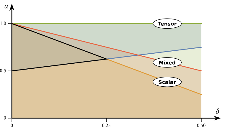
Figure 1: The space of parameters $\alpha$ and $\delta$ determining the Lagrangian functions (18). The region above the blue line corresponds to the parameters which yield the Minkowski spacetime as $t\to-\infty$ and evade the no-go theorem of Ref. [18]. The area below the green line ($\alpha<1$) is the region free of the strong coupling problem inferred from the tensor sector analysis at the cubic level. Similarly, regions below the red ($\alpha<1-\delta$) and orange ($2\alpha<2-3\delta$) lines are obtained by the analysis of the mixed and scalar sectors, respectively. The black-framed area shows the allowed range of the parameters $\alpha$ and $\delta$ free of the strong coupling problem inferred from the analysis of all cubic interactions and free of instabilities.

4 Conclusion

We have studied the nonsingular genesis scenario in the framework of the Horndeski theory, which is capable of avoiding the gradient instability at the expense of potential strong coupling problem. The model of genesis presented in Ref. [18] has been used as an example that gives an explicit asymptotic solution at early times ($t\to-\infty$). The parameters $\alpha$ and $\delta$ that determine the Lagrangian of this model were chosen in the range consistent with stable genesis, i.e., violation of the no-go theorem [18].

We have seen that with the additional restrictions on $\alpha$ and $\delta$, the classical genesis solution is away from the strong coupling regime inferred from the study of all cubic interactions of metric perturbations: scalar, mixed and tensor. These restrictions came from the requirement that all characteristic energy scales, associated with cubic action, must be larger than the classical energy scale (in our model it is $E_{class}\propto\dot{H}/H$). This opens up the possibility that the Universe starts up with very low quantum gravity energy scale (the effective Planck mass asymptotically vanishes as $t\to-\infty$), and yet its classical evolution is so slow that the classical field theory description remains valid. We presented the healthy region of parameters $\alpha$ and $\delta$ in Fig.1.

In Appendix B we also noted a non-trivial point concerning the strong coupling regime in models with singular metric. Namely, in that case, healthy behavior of the coefficients in the quadratic action does not necessarily imply that the classical treatment of the background evolution is legitimate.

Even though our analysis has led to a promising outcome, it is certainly incomplete, as there is no guarantee that the fourth and higher order interactions will give strong coupling energy scales higher than or equal to the ones we have found by studying the cubic interactions. We plan to turn to this issue in the future.

Appendix A Explicit expressions used in the second and third order calculations

In this Appendix, we give complete expressions for Lagrangians which are quadratic and cubic in metric perturbations in the unitary gauge. These expressions are valid in the general Horndeski theory whose Lagrangian is

$$\mathcal{L} = G_{2}(\phi,X)-G_{3}(\phi,X)\Box\phi+G_{4}(\phi,X)R+G_{4X}\left[(\Box\phi)^{2}-(\nabla_{\mu}\nabla_{\nu}\phi)^{2}\right]$$ (54)

$$+G_{5}(\phi,X)G_{\mu\nu}\nabla^{\mu}\nabla^{\nu}\phi-\frac{1}{6}G_{5X}\bigl{[}(\Box\phi)^{3}-3\Box\phi(\nabla_{\mu}\nabla_{\nu}\phi)^{2}+2(\nabla_{\mu}\nabla_{\nu}\phi)^{3}\bigr{]}.$$

In each of the sectors, after writing the general expressions, we specify to our particular model (6) and (18).

Second-order Lagrangian in the scalar sector

We start with the second-order Lagrangian. In the scalar sector we have

$$N=1+\alpha\;,\;\;\;\;N_{i}=\partial_{i}\beta\;,\;\;\;\;\gamma_{ij}=a^{2}e^{2\zeta}\delta_{ij}\;.$$ (55)

The quadratic Lagrangian for perturbations reads [40]

$$\mathcal{L}_{ss}=a^{3}\left[-3\mathcal{G}_{T}\frac{\dot{\zeta}^{2}}{N^{2}}+\frac{\mathcal{F}_{T}}{a^{2}}\zeta_{,i}\zeta_{,i}+\Sigma\alpha^{2}-\frac{2}{a^{2}}\Theta\alpha\beta_{,ii}+\frac{2}{a^{2}}\mathcal{G}_{T}\frac{\dot{\zeta}}{N}\beta_{,ii}+6\Theta\alpha\frac{\dot{\zeta}}{N}-\frac{2}{a^{2}}\mathcal{G}_{T}\alpha\zeta_{,ii}\right],$$ (56)

where

$$\mathcal{F}_{T} = 2\left[G_{4}-X\left(\frac{\ddot{\phi}}{N^{2}}G_{5X}+G_{5\phi}\right)\right],$$ (57a)

$$\mathcal{G}_{T} = 2\left[G_{4}-2XG_{4X}-X\left(H\frac{\dot{\phi}}{N}G_{5X}-G_{5\phi}\right)\right],$$ (57b)

$$\Sigma = XG_{2X}+2X^{2}G_{2XX}+12H\frac{\dot{\phi}}{N}XG_{3X}+6H\frac{\dot{\phi}}{N}X^{2}G_{3XX}-2XG_{3\phi}-2X^{2}G_{3\phi X}$$ (58a)

$$-6H^{2}G_{4}+6\Bigg{[}H^{2}\left(7XG_{4X}+16X^{2}G_{4XX}+4X^{3}G_{4XXX}\right)$$

$$-H\frac{\dot{\phi}}{N}\left(G_{4\phi}+5XG_{4\phi X}+2X^{2}G_{4\phi XX}\right)\Bigg{]}$$

$$+30H^{3}\frac{\dot{\phi}}{N}XG_{5X}+26H^{3}\frac{\dot{\phi}}{N}X^{2}G_{5XX}+4H^{3}\frac{\dot{\phi}}{N}X^{3}G_{5XXX}$$

$$-6H^{2}X\left(6G_{5\phi}+9XG_{5\phi X}+2X^{2}G_{5\phi XX}\right),$$

$$\Theta = -\frac{\dot{\phi}}{N}XG_{3X}+2HG_{4}-8HXG_{4X}-8HX^{2}G_{4XX}+\frac{\dot{\phi}}{N}G_{4\phi}+2X\frac{\dot{\phi}}{N}G_{4\phi X}$$ (58b)

$$-H^{2}\frac{\dot{\phi}}{N}\left(5XG_{5X}+2X^{2}G_{5XX}\right)+2HX\left(3G_{5\phi}+2XG_{5\phi X}\right).$$

Variation of this action with respect to the Lagrange multipliers $\alpha$ and $\beta$ leads to the linearized constraint equations

$$\Sigma\alpha-\frac{\Theta}{a^{2}}\partial^{2}\beta+3\Theta\frac{\dot{\zeta}}{N}-\frac{\mathcal{G}_{T}}{a^{2}}\partial^{2}\zeta = 0,$$ (59a)

$$\Theta\alpha-\mathcal{G}_{T}\frac{\dot{\zeta}}{N} = 0.$$ (59b)

The solution to these equations is

$$\alpha = \frac{\mathcal{G}_{T}}{\Theta}\frac{\dot{\zeta}}{N},$$ (60a)

$$\beta = \frac{1}{a\mathcal{G}_{T}}\left(a^{3}\mathcal{G}_{S}\psi-\frac{a\mathcal{G}_{T}^{2}}{\Theta}\zeta\right)\;.$$ (60b)

Upon inserting these expressions into (56), one finds [42] that the unconstrained second-order action for the scalar metric perturbation $\zeta$ is given by Eq. (1), where the coefficients have the following form:

$$\mathcal{F}_{S} = \frac{1}{a}\frac{d}{dt}\left(\frac{a}{\Theta}\mathcal{G}_{T}^{2}\right)-\mathcal{F}_{T},$$ (61a)

$$\mathcal{G}_{S} = \frac{\Sigma}{\Theta^{2}}\mathcal{G}_{T}^{2}+3\mathcal{G}_{T}.$$ (61b)

The sound speed is given by $c_{s}^{2}=\mathcal{F}_{S}/\mathcal{G}_{S}$.

For our specific Lagrangian (6) with $G_{4}=G_{4}(\phi)$ and $G_{5}(\phi,X)=0$, expressions (57) have the form of (17), while for $\Sigma$ and $\Theta$ we have the following expressions:

$$\Sigma = XG_{2X}+2X^{2}G_{2XX}+12H\frac{\dot{\phi}}{N}XG_{3X}+6H\frac{\dot{\phi}}{N}X^{2}G_{3XX}-2XG_{3\phi}-2X^{2}G_{3\phi X}$$ (62a)

$$-6H^{2}G_{4}-6H\frac{\dot{\phi}}{N}G_{4\phi},$$

$$\Theta = -\frac{\dot{\phi}}{N}XG_{3X}+2HG_{4}+\frac{\dot{\phi}}{N}G_{4\phi}.$$ (62b)

In 3+1 formalism these formulas read

$$\Sigma = -3H^{2}\left[B_{4}-\frac{1}{6H^{2}}\left(A_{2}+3NA_{2N}+N^{2}A_{2NN}\right)-\frac{1}{2H}\left(NA_{3N}+N^{2}A_{3NN}\right)\right],$$ (63a)

$$\Theta = 2H\left(\frac{NA_{3N}}{4H}+B_{4}\right),$$ (63b)

where we use the relation $\sqrt{2X}=\frac{1}{(-t)N}$ which is obtained from the gauge condition (10). The asymptotic behavior of the coefficients in the model (18) is given by Eq. (28), and we use in what follows the asymptotics

$$\Sigma\propto(-t)^{-2\alpha-\delta-2},\;\;\;\;\;\;\;\Theta\propto(-t)^{-2\alpha-\delta-1}.$$ (64)

Third-order action

Scalar sector

Complete third-order action for scalars $\alpha$, $\beta$ and $\zeta$ is given in [38, 39, 40] and has the following form:

$$\mathcal{L}_{sss} = -\frac{a^{3}}{3}\left(\Sigma+2X\Sigma_{X}+H\Xi\right)\alpha^{3}+a^{3}\left[3\Sigma\zeta+\Xi\frac{\dot{\zeta}}{N}+\left(\Gamma-\mathcal{G}_{T}\right)\frac{\zeta_{,ii}}{a^{2}}-\frac{\Xi}{3a^{2}}\beta_{,ii}\right]\alpha^{2}$$ (65)

$$-2a\Theta\alpha\zeta_{,i}\beta_{,i}+18a^{3}\Theta\alpha\zeta\frac{\dot{\zeta}}{N}+4a\mu\alpha\frac{\dot{\zeta}}{N}\zeta_{,ii}-\frac{\Gamma}{2a}\alpha\left(\beta_{,ij}\beta_{,ij}-\beta_{,ii}\beta_{,jj}\right)$$

$$+\frac{2\mu}{a}\alpha\left(\beta_{,ij}\zeta_{,ij}-\beta_{,ii}\zeta_{,jj}\right)-2a\Theta\alpha\beta_{,ii}\zeta-2a\Gamma\alpha\beta_{,ii}\frac{\dot{\zeta}}{N}-2a\mathcal{G}_{T}\alpha\zeta\zeta_{,ii}-a\mathcal{G}_{T}\alpha\zeta_{,i}\zeta_{,i}$$

$$+3a^{3}\Gamma\alpha\frac{\dot{\zeta}^{2}}{N^{2}}+2a^{3}\mu\frac{\dot{\zeta}^{3}}{N^{3}}+a\mathcal{F}_{T}\zeta\zeta_{,i}\zeta_{,i}-9a^{3}\mathcal{G}_{T}\frac{\dot{\zeta}^{2}}{N^{2}}\zeta+2a\mathcal{G}_{T}\beta_{,i}\zeta_{,i}\frac{\dot{\zeta}}{N}-2a\mu\beta_{ii}\frac{\dot{\zeta}^{2}}{N^{2}}$$

$$+2a\mathcal{G}_{T}\beta_{,ii}\frac{\dot{\zeta}}{N}\zeta+\frac{1}{a}\left(\frac{3}{2}\mathcal{G}_{T}\zeta-\mu\frac{\dot{\zeta}}{N}\right)\left(\beta_{,ij}\beta_{,ij}-\beta_{,ii}\beta_{,jj}\right)-2\frac{\mathcal{G}_{T}}{a}\beta_{,ii}\beta_{,j}\zeta_{,j},$$

where

$$\Xi = 12\frac{\dot{\phi}}{N}XG_{3X}+6\frac{\dot{\phi}}{N}X^{2}G_{3XX}-12HG_{4}$$ (66)

$$+6\left[2H\left(7XG_{4X}+16X^{2}G_{4XX}+4X^{3}G_{4XXX}\right)-\frac{\dot{\phi}}{N}\left(G_{4\phi}+5XG_{4\phi X}+2X^{2}G_{4\phi XX}\right)\right]$$

$$+90H^{2}\frac{\dot{\phi}}{N}XG_{5X}+78H^{2}\frac{\dot{\phi}}{N}X^{2}G_{5XX}+12H^{2}\frac{\dot{\phi}}{N}X^{3}G_{5XXX}$$

$$-12HX\left(6G_{5\phi}+9XG_{5\phi X}+2X^{2}G_{5\phi XX}\right),$$

$$\Gamma = 2G_{4}-8XG_{4X}-8X^{2}G_{4XX}$$ (67)

$$-2H\frac{\dot{\phi}}{N}\left(5XG_{5X}+2X^{2}G_{5XX}\right)+2X\left(3G_{5\phi}+2XG_{5\phi X}\right),$$

$$\mu=\frac{\dot{\phi}}{N}XG_{5X}.$$ (68)

We insert solutions (60) to the constraints into the Lagrangian (65) and find the unconstrained cubic Lagrangian for $\zeta$. The expressions for the coefficients of the 17 terms in formula (30) are given by (in square brackets we also show the interaction type for convenience)

$$\begin{array}[]{*2{>{\displaystyle}r>{\displaystyle}l}}\Lambda_{1}[\dot{\zeta}^{3}/N^{3}]&\lx@intercol\displaystyle=-\frac{\mathcal{G}_{T}^{3}}{3\Theta^{3}}(\Sigma+2X\Sigma_{X}+H\Xi)+\frac{\mathcal{G}_{T}^{2}\Xi}{\Theta^{2}}-\frac{\mathcal{G}_{T}\mathcal{G}_{S}\Xi}{3\Theta^{2}}+\frac{\Gamma\mathcal{G}_{S}^{2}}{2\Theta\mathcal{G}_{T}}\hfil\lx@intercol\\ \hfil&\lx@intercol\displaystyle\phantom{=}-\frac{2\Gamma\mathcal{G}_{S}}{\Theta}+\frac{3\Gamma\mathcal{G}_{T}}{\Theta}+\mu\Big{(}2-2\frac{\mathcal{G}_{S}}{\mathcal{G}_{T}}+\frac{\mathcal{G}_{S}^{2}}{\mathcal{G}_{T}^{2}}\Big{)},\hfil\lx@intercol&\\ \Lambda_{2}[(\dot{\zeta}^{2}/N^{2})\zeta]&\lx@intercol\displaystyle=\frac{3\mathcal{G}_{T}^{2}\Sigma}{\Theta^{2}}+9\mathcal{G}_{T}-\frac{3\mathcal{G}_{S}^{2}}{2\mathcal{G}_{T}},\hfil\lx@intercol&\\ \Lambda_{3}[(\dot{\zeta}^{2}/N^{2})\partial^{2}\zeta]&\lx@intercol\displaystyle=\frac{\mathcal{G}_{T}^{3}\Xi}{3a^{2}\Theta^{3}}-\frac{\mathcal{G}_{T}\mathcal{G}_{S}\Gamma}{a^{2}\Theta^{2}}+\frac{2\Gamma\mathcal{G}_{T}^{2}}{a^{2}\Theta^{2}}+\frac{\mu}{a^{2}}\Big{(}6\frac{\mathcal{G}_{T}}{\Theta}-4\frac{\mathcal{G}_{S}}{\Theta}\Big{)},\hfil\lx@intercol&\\ \Lambda_{4}[(\dot{\zeta}/N)\zeta\partial^{2}\zeta]&=\frac{3\mathcal{G}_{T}\mathcal{G}_{S}}{a^{2}\Theta}-\frac{2\mathcal{G}_{T}^{2}}{a^{2}\Theta},&\Lambda_{5}[(\dot{\zeta}/N)\left(\partial_{i}\zeta\right)^{2}]&=-\frac{\mathcal{G}_{T}^{2}}{a^{2}\Theta}+\frac{2\mathcal{G}_{T}\mathcal{G}_{S}}{a^{2}\Theta},\\ \Lambda_{6}[\zeta\left(\partial_{i}\zeta\right)^{2}]&=\frac{\mathcal{F}_{T}}{a^{2}},&\Lambda_{7}[(\dot{\zeta}/N)\left(\partial^{2}\zeta\right)^{2}]&=\frac{\Gamma\mathcal{G}_{T}^{3}}{2a^{4}\Theta^{3}}+3\frac{\mu\mathcal{G}_{T}^{2}}{a^{4}\Theta^{2}},\\ \Lambda_{8}[\zeta\left(\partial^{2}\zeta\right)^{2}]&=-\frac{3\mathcal{G}_{T}^{3}}{2a^{4}\Theta^{2}},&\Lambda_{9}[\partial^{2}\zeta\left(\partial_{i}\zeta\right)^{2}]&=-\frac{2\mathcal{G}_{T}^{3}}{a^{4}\Theta^{2}},\\ \Lambda_{10}[(\dot{\zeta}/N)\big{(}\partial_{i}\partial_{j}\zeta\big{)}^{2}]&=-\frac{\Gamma\mathcal{G}_{T}^{3}}{2a^{4}\Theta^{3}}-3\frac{\mu\mathcal{G}_{T}^{2}}{a^{4}\Theta^{2}},&\Lambda_{11}[\zeta\big{(}\partial_{i}\partial_{j}\zeta\big{)}^{2}]&=\frac{3\mathcal{G}_{T}^{3}}{2a^{4}\Theta^{2}},\\ \Lambda_{12}[(\dot{\zeta}/N)\partial_{i}\zeta\partial^{i}\psi]&=-\frac{2\mathcal{G}_{S}^{2}}{\mathcal{G}_{T}},&\Lambda_{13}[\partial^{2}\zeta\partial_{i}\zeta\partial^{i}\psi]&=\frac{2\mathcal{G}_{T}\mathcal{G}_{S}}{a^{2}\Theta},\\ \Lambda_{14}[(\dot{\zeta}/N)\big{(}\partial_{i}\partial_{j}\psi\big{)}^{2}]&=-\frac{\Gamma\mathcal{G}_{S}^{2}}{2\Theta\mathcal{G}_{T}}-\frac{\mu\mathcal{G}_{S}^{2}}{\mathcal{G}_{T}^{2}},&\Lambda_{15}[\zeta\big{(}\partial_{i}\partial_{j}\psi\big{)}^{2}]&=\frac{3\mathcal{G}_{S}^{2}}{2\mathcal{G}_{T}},\\ \Lambda_{16}[(\dot{\zeta}/N)\partial_{i}\partial_{j}\zeta\partial^{i}\partial^{j}\psi]&=\frac{\mathcal{G}_{T}\mathcal{G}_{S}\Gamma}{a^{2}\Theta^{2}}+4\frac{\mu\mathcal{G}_{S}}{a^{2}\Theta},&\Lambda_{17}[\zeta\partial_{i}\partial_{j}\zeta\partial^{i}\partial^{j}\psi]&=-\frac{3\mathcal{G}_{T}\mathcal{G}_{S}}{a^{2}\Theta}.\end{array}$$

For our specific model (6) and (18) we have

$$\Xi = 12\frac{\dot{\phi}}{N}XG_{3X}+6\frac{\dot{\phi}}{N}X^{2}G_{3XX}-12HG_{4}-6\frac{\dot{\phi}}{N}G_{4\phi},$$ (70a)

$$\Gamma = \mathcal{G}_{T}=\mathcal{F}_{T}=2G_{4},$$ (70b)

$$\mu = 0.$$ (70c)

In ADM formalism we have

$$\Xi=A_{3}+\frac{3}{2}N^{2}A_{3NN}-12HB_{4},\;\;\;\Gamma=2B_{4}\;.$$ (71)

The asymptotic behavior of these combinations is

$$\Xi\propto(-t)^{-2\alpha-1-\delta},\;\;\;\Gamma\propto(-t)^{-2\alpha}.$$ (72)

Making use of these expressions, we find the early-time asymptotics of all $\Lambda_{i}$, listed in Table LABEL:scalarcondtab.

Mixed sectors

First, let us turn to the case of two tensors and one scalar. One has [40]

$$d_{1} = \frac{3\mathcal{G}_{T}}{8}\left[1-\frac{H\mathcal{G}_{T}^{2}}{\Theta\mathcal{F}_{T}}+\frac{\mathcal{G}_{T}}{3}\frac{d}{Ndt}\left(\frac{\mathcal{G}_{T}}{\Theta\mathcal{F}_{T}}\right)\right],$$ (73a)

$$d_{2} = \frac{\mathcal{F}_{S}}{8},$$ (73b)

$$d_{3} = -\frac{\mathcal{G}_{S}}{4},$$ (73c)

$$d_{4} = \frac{\mathcal{G}_{T}}{8\Theta\mathcal{F}_{T}}\left(\mathcal{G}_{T}^{2}-\Gamma\mathcal{F}_{T}\right)$$ (73d)

$$+ \frac{\mu}{4}\left[\frac{\mathcal{G}_{S}}{\mathcal{G}_{T}}-1-\frac{H\mathcal{G}_{T}^{2}}{\Theta\mathcal{F}_{T}}\left(6+\frac{\dot{\mathcal{G}}_{S}}{NH\mathcal{G}_{S}}\right)\right]+\frac{\mathcal{G}_{T}^{2}}{4}\frac{d}{Ndt}\left(\frac{\mu}{\Theta\mathcal{F}_{T}}\right),$$

$$d_{5} = \frac{\mu\mathcal{G}_{T}}{4\Theta}\left(\frac{\mathcal{F}_{S}\mathcal{G}_{T}}{\mathcal{F}_{T}\mathcal{G}_{S}}-1\right)\;,$$ (73e)

$$d_{6} = -\frac{\mu}{2}\frac{\mathcal{G}_{S}}{\mathcal{G}_{T}}\;,$$ (73f)

$$d_{7} = \frac{\mu}{2}\frac{\mathcal{G}_{T}}{\Theta}\;.$$ (73g)

Several coefficients vanish due to (70):

$$d_{4}=d_{5}=d_{6}=d_{7}=0.$$

The asymptotics of the remaining coefficients are given in Table LABEL:crosscondtab.

We now write formulas for two scalar and one tensor case [40]:

$$c_{1} = \mathcal{F}_{S},$$ (74a)

$$c_{2} = \frac{\Gamma}{4\Theta}\left(\mathcal{F}_{S}-\mathcal{F}_{T}\right)+\frac{\mathcal{G}_{T}^{2}}{\Theta}\left[-\frac{1}{2}+\frac{H\Gamma}{4\Theta}\left(3+\frac{\dot{\mathcal{G}}_{T}}{NH\mathcal{G}_{T}}\right)-\frac{1}{4}\frac{d}{Ndt}\left(\frac{\Gamma}{\Theta}\right)\right]$$ (74b)

$$+\frac{\mu\mathcal{F}_{S}}{\mathcal{G}_{T}}+\frac{2H\mathcal{G}_{T}\mu}{\Theta}-\mathcal{G}_{T}\frac{d}{Ndt}\left(\frac{\mu}{\Theta}\right),$$

$$c_{3} = \mathcal{G}_{S}\left[\frac{3}{2}+\frac{d}{Ndt}\left(\frac{\Gamma}{2\Theta}+\frac{\mu}{\mathcal{G}_{T}}\right)-\left(3H+\frac{\dot{\mathcal{G}}_{T}}{N\mathcal{G}_{T}}\right)\left(\frac{\Gamma}{2\Theta}+\frac{\mu}{\mathcal{G}_{T}}\right)\right],$$ (74c)

$$c_{4} = \mathcal{G}_{S}\left[-\frac{\mathcal{G}_{T}^{2}-\Gamma\mathcal{F}_{T}}{2\Theta\mathcal{G}_{T}}-\frac{2H\mu}{\Theta}+\frac{d}{Ndt}\left(\frac{\mu}{\Theta}\right)+\frac{\mu}{\mathcal{G}_{T}^{2}}\left(\mathcal{F}_{T}-\mathcal{F}_{S}\right)\right],$$ (74d)

$$c_{5} = \frac{\mathcal{G}_{T}^{2}}{2\Theta}\left[\frac{\mathcal{G}_{T}^{2}-\Gamma\mathcal{F}_{T}}{2\Theta\mathcal{G}_{T}}+\frac{2H\mu}{\Theta}-\frac{d}{Ndt}\left(\frac{\mu}{\Theta}\right)-\frac{\mu}{\mathcal{G}_{T}^{2}}\left(3\mathcal{F}_{T}-\mathcal{F}_{S}\right)\right],$$ (74e)

$$c_{6} = \frac{\mathcal{G}_{S}^{2}}{4\mathcal{G}_{T}}\left[1+\frac{6H\mu}{\mathcal{G}_{T}}-2\mathcal{G}_{T}\frac{d}{Ndt}\left(\frac{\mu}{\mathcal{G}_{T}^{2}}\right)\right].$$ (74f)

We again make use of (70) and obtain

$$c_{4}=c_{5}=0.$$

Other coefficients have asymptotics listed in Table LABEL:crosscondtab.

Appendix B Einstein frame: strong coupling problem in models with singular metric

In this Appendix we point out that when dealing with singular metric, one should keep in mind the potential strong coupling problem, even if it does not show up at quadratic order. To this end, we consider the theory (6) and make the conformal transformation of the metric:

$$\tilde{g}_{\mu\nu}=\Omega(\phi)g_{\mu\nu},$$ (75)

where $\Omega(\phi)$ is a conformal factor. The new metric has the standard FLRW form $\tilde{ds^{2}}=-\tilde{N}^{2}dt^{2}+\tilde{a}^{2}dx^{2}$, where

$$\tilde{N}^{2}=\Omega N^{2},\hskip 14.22636pt\tilde{a}^{2}=\Omega a^{2},$$ (76)

We take $\Omega(\phi)=2G_{4}(\phi)/M^{2}_{Pl}$ and thus move from the Jordan frame and the Lagrangian (6) to the Einstein frame and the Lagrangian

$$\cal\tilde{L} = \tilde{G}_{2}(\phi,\tilde{X})-\tilde{G}_{3}(\phi,\tilde{X})\tilde{\Box}\phi+\frac{M_{Pl}^{2}}{2}\tilde{R},$$ (77)

with $\tilde{X}=-\frac{1}{2}\tilde{g}^{\mu\nu}\tilde{\partial}_{\mu}\phi\tilde{\partial}_{\nu}\phi$, $\tilde{\Box}\phi=\tilde{g}^{\mu\nu}\tilde{\nabla}_{\mu}\tilde{\nabla}_{\nu}\phi$, where the functions $\tilde{G}_{2}$, $\tilde{G}_{3}$ and $\tilde{G}_{4}$ are combinations of the Jordan frame $G_{2},G_{3}$ and $G_{4}$, and $\tilde{R}$ is the Ricci scalar for the metric $\tilde{g}_{\mu\nu}$.

Since $G_{4}=B_{4}$ is given by (18c), it is straightforward to find the asymptotics of the Einstein frame background solution in terms of cosmic time $\tau\propto\int\sqrt{\Omega}Ndt\propto-(-t)^{1-\alpha}$. We consider the case $\alpha<1$, in which strong coupling is absent in the tensor sector, and get

$$\tilde{a} \propto\frac{1}{(-\tau)^{\alpha/(1-\alpha)}},$$ (78a)

$$\tilde{H} \propto\frac{1}{(-\tau)},$$ (78b)

$$e^{\phi} \propto\frac{1}{(-\tau)^{1/(1-\alpha)}}\;.$$ (78c)

The cosmological evolution starts at $\tau\to-\infty$. Notably, the metric is singular in this asymptotics, $\tilde{a}\to 0$ as $\tau\to-\infty$, but the Hubble parameter and its derivatives vanish. A similar solution was called “modified genesis” in Ref. [17], where it was assumed that such solutions are healthy. The analysis of this paper shows, however, that this is not necessarily the case: away from the solid triangle and above the blue line in Fig. 1, our model suffers from the strong coupling problem. Indeed, the range of parameters in which the model is healthy (not healthy) is invariant under field redefinition (conformal transformation in our case).

To emphasize the subtlety of the situation, let us consider linearized theory in the Einstein frame. The metric is

$$d\tilde{s}^{2}=-\tilde{N}^{2}dt^{2}+\tilde{\gamma}_{ij}\left(dx^{i}+\tilde{N}^{i}dt\right)\left(dx^{j}+\tilde{N}^{j}dt\right),$$ (79)

where

$$\tilde{\gamma}_{ij}=\tilde{a}^{2}e^{2\zeta}\left(e^{h}\right)_{ij},\;\;\;\delta\tilde{N}=\tilde{N}\tilde{\alpha},\;\;\;\delta\tilde{N}_{i}=\partial_{i}\tilde{\beta}$$ (80)

and thus

$$\tilde{\alpha}=\alpha,\;\;\;\tilde{\beta}=\beta/\sqrt{\Omega},\;\;\;\tilde{\zeta}=\zeta.$$ (81)

The scalar perturbation $\tilde{\zeta}=\zeta$ has the same action as in the Jordan frame, so in terms of the Einstein frame variables one has

$$\tilde{\mathcal{S}}_{ss}=\int\tilde{N}dt\tilde{a}^{3}d^{3}x\left[\tilde{\mathcal{G}}_{S}\frac{\dot{\zeta}^{2}}{\tilde{N}^{2}}-\frac{\tilde{\mathcal{F}}_{S}}{\tilde{a}^{2}}\zeta_{,i}\zeta_{,i}\right],$$ (82)

where

$$\tilde{\mathcal{G}}_{S}=\frac{\mathcal{G}_{S}}{\Omega},\;\;\;\tilde{\mathcal{F}}_{S}=\frac{\mathcal{F}_{S}}{\Omega}.$$ (83)

The asymptotic behavior of the latter coefficients is

$$\tilde{\mathcal{G}}_{S}\propto(-\tau)^{\delta/1-\alpha},\;\;\;\tilde{\mathcal{F}}_{S}\propto(-\tau)^{\delta/1-\alpha}\;.$$ (84)

Unlike in the Jordan frame, these coefficients tend to $\infty$ as $\tau\to-\infty$. Naively, this behavior suggests that not only is there no danger of strong coupling, but the theory becomes free in the asymptotic past. Were the background metric nonsingular, this would indeed be the case. In our model with a singular Einstein frame metric, the naive expectation fails: the model is strongly coupled as $\tau\to-\infty$ (away from the solid triangle and above the blue line in Fig. 1). We conclude that in models with a singular metric, the study of the quadratic action for perturbations is insufficient for analyzing the strong coupling problem.

References

- [1] P. Creminelli, A. Nicolis and E. Trincherini, JCAP 1011, 021 (2010).
- [2] P. Creminelli, K. Hinterbichler, J. Khoury, A. Nicolis and E. Trincherini, JHEP 1302, 006 (2013).
- [3] K. Hinterbichler, A. Joyce, J. Khoury and G. E. J. Miller, JCAP 1212, 030 (2012).
- [4] K. Hinterbichler, A. Joyce, J. Khoury and G. E. J. Miller, Phys. Rev. Lett. 110, no. 24, 241303 (2013).
- [5] S. Nishi and T. Kobayashi, JCAP 1503, 057 (2015).
- [6] F. J. Tipler, Phys. Rev. D 17, 2521 (1978).
- [7] G. W. Horndeski, Int. J. Theor. Phys. 10, 363 (1974).
- [8] D. B. Fairlie, J. Govaerts and A. Morozov, Nucl. Phys. B 373, 214 (1992).
- [9] M. A. Luty, M. Porrati and R. Rattazzi, JHEP 0309, 029 (2003).
- [10] A. Nicolis and R. Rattazzi, JHEP 0406, 059 (2004).
- [11] A. Nicolis, R. Rattazzi and E. Trincherini, Phys. Rev. D 79, 064036 (2009).
- [12] C. Deffayet, O. Pujolas, I. Sawicki and A. Vikman, JCAP 1010, 026 (2010).
- [13] T. Kobayashi, M. Yamaguchi and J. Yokoyama, Phys. Rev. Lett. 105, 231302 (2010).
- [14] A. Padilla and V. Sivanesan, JHEP 1304, 032 (2013).
- [15] T. Kobayashi, Rept. Prog. Phys. 82, no. 8, 086901 (2019).
- [16] V. A. Rubakov, Phys. Usp. 57, 128 (2014) [Usp. Fiz. Nauk 184, no. 2, 137 (2014)].
- [17] M. Libanov, S. Mironov and V. Rubakov, JCAP 1608, 037 (2016).
- [18] T. Kobayashi, Phys. Rev. D 94, no. 4, 043511 (2016).
- [19] R. Kolevatov and S. Mironov, Phys. Rev. D 94, no. 12, 123516 (2016).
- [20] S. Akama and T. Kobayashi, Phys. Rev. D 95, no. 6, 064011 (2017).
- [21] Y. Cai, Y. Wan, H. G. Li, T. Qiu and Y. S. Piao, JHEP 1701, 090 (2017).
- [22] P. Creminelli, D. Pirtskhalava, L. Santoni and E. Trincherini, JCAP 1611, 047 (2016).
- [23] R. Kolevatov, S. Mironov, N. Sukhov and V. Volkova, JCAP 1708, 038 (2017).
- [24] M. Zumalacárregui and J. García-Bellido, Phys. Rev. D 89, 064046 (2014).
- [25] J. Gleyzes, D. Langlois, F. Piazza and F. Vernizzi, Phys. Rev. Lett. 114, no. 21, 211101 (2015).
- [26] S. Mironov, V. Rubakov and V. Volkova, Phys. Rev. D 100, no. 8, 083521 (2019).
- [27] A. Ijjas and P. J. Steinhardt, Phys. Lett. B 764, 289 (2017).
- [28] S. Nishi and T. Kobayashi, Phys. Rev. D 95, no. 6, 064001 (2017).
- [29] Y. Ageeva, O. Evseev, O. Melichev and V. Rubakov, EPJ Web Conf. 191, 07010 (2018).
- [30] A. Borde, A. H. Guth and A. Vilenkin, Phys. Rev. Lett. 90, 151301 (2003).
- [31] G. Papallo and H. S. Reall, Phys. Rev. D 96, no. 4, 044019 (2017).
- [32] Á. D. Kovács and H. S. Reall, Phys. Rev. D 101, no. 12, 124003 (2020).
- [33] J. Gleyzes, D. Langlois, F. Piazza and F. Vernizzi, JCAP 1308, 025 (2013).
- [34] M. Fasiello and S. Renaux-Petel, JCAP 1410, 037 (2014).
- [35] T. Kobayashi, M. Yamaguchi and J. Yokoyama, JCAP 1507, 017 (2015).
- [36] G. Cusin, M. Lewandowski and F. Vernizzi, JCAP 1804, 061 (2018).
- [37] A. De Felice, T. Kobayashi and S. Tsujikawa, Phys. Lett. B 706, 123 (2011).
- [38] X. Gao and D. A. Steer, JCAP 1112, 019 (2011).
- [39] A. De Felice and S. Tsujikawa, Phys. Rev. D 84, 083504 (2011).
- [40] X. Gao, T. Kobayashi, M. Shiraishi, M. Yamaguchi, J. Yokoyama and S. Yokoyama, PTEP 2013, 053E03 (2013).
- [41] X. Gao, T. Kobayashi, M. Yamaguchi and J. Yokoyama, Phys. Rev. Lett. 107, 211301 (2011).
- [42] T. Kobayashi, M. Yamaguchi and J. Yokoyama, Prog. Theor. Phys. 126, 511 (2011).
- [43] X. Chen, M. x. Huang, S. Kachru and G. Shiu, JCAP 0701, 002 (2007).