Electron-positron annihilation into two photons in an intense plane-wave field

Abstract

The process of electron-positron annihilation into two photons in the presence of an intense classical plane wave of an arbitrary shape is investigated analytically by employing light-cone quantization and by taking into account the effects of the plane wave exactly. We introduce a general description of second-order 2-to-2 scattering processes in a plane-wave background field, indicating the necessity of considering the localization of the colliding particles and achieving that by means of wave packets. We define a local cross section in the background field, which generalizes the vacuum cross section and which, though not being directly an observable, allows for a comparison between the results in the plane wave and in vacuum without relying on the shape of the incoming wave packets. Two possible cascade or two-step channels have been identified in the annihilation process and an alternative way of representing the two-step and one-step contributions via a “virtuality” integral has been found. Finally, we compute the total local cross section to leading order in the coupling between the electron-positron field and the quantized photon field, excluding the interference between the two leading-order diagrams arising from the exchange of the two final photons, and express it in a relatively compact form. In contrast to processes in a background field initiated by a single particle, the pair annihilation into two photons, in fact, also occurs in vacuum. Our result naturally embeds the vacuum part and reduces to the vacuum expression, known in the literature, in the case of a vanishing laser field.

I Introduction

With the development of high-power laser technology the verification of the nonlinear-QED predictions for various phenomena in an intense background field of a macroscopic extent is becoming attainable in laboratory experiments Marklund and Shukla (2006); Ehlotzky et al. (2009); Di Piazza et al. (2012); Narozhny and Fedotov (2015); King and Heinzl (2016). Among QED processes in an intense laser field, two first-order ones, nonlinear Compton scattering ($e^{-}\Rightarrow e^{-}\gamma$) Brown and Kibble (1964); Neville and Rohrlich (1971); Ritus (1985); Ivanov et al. (2004); Harvey et al. (2009); Boca and Florescu (2009); Mackenroth et al. (2010); Seipt and Kämpfer (2011); Mackenroth and Di Piazza (2011); Krajewska and Kamiński (2012a); Wistisen (2014); Angioi et al. (2016); Wistisen and Di Piazza (2019) and nonlinear Breit-Wheeler pair production ($\gamma\Rightarrow e^{-}e^{+}$) Reiss (1962); Ritus (1985); Bulanov et al. (2010); Heinzl et al. (2010); Ipp et al. (2011); Krajewska and Kamiński (2012b); Jansen and Müller (2013); Fedotov and Mironov (2013); Meuren et al. (2015) have been extensively investigated theoretically (see also the reviews Mitter (1975); Ehlotzky et al. (2009); Di Piazza et al. (2012); Narozhny and Fedotov (2015)), where by a double-line arrow we highlight the fact that a process happens in a background field, which in general has to be taken into account nonperturbatively. Recently, nonlinear Compton scattering was also probed experimentally and signatures of quantum effects were observed Cole et al. (2018); Poder et al. (2018) (see Ref. Wistisen et al. (2018) for a related experiment carried out in crystals). Moreover, these reactions are the only QED effects included in common implementations of the QED particle-in-cell (PIC) scheme Arber et al. (2015); Gonoskov et al. (2015); Lobet et al. (2016), which is a standard tool for the numerical investigation of the interaction between a laser field of extreme intensity ($\gtrsim 10^{23}$ W/cm²) and matter, in particular, of the dynamics of the electron-positron plasma, produced in this interaction Bell and Kirk (2008); Nerush et al. (2011); Ridgers et al. (2012); Jirka et al. (2016); Grismayer et al. (2016); Tamburini et al. (2017); Vranic et al. (2017); Luo et al. (2018); Efimenko et al. (2018, 2019) (an electron-positron plasma interacting with a background field can also arise in a collision of a high-density electron beam with a target Sarri et al. (2015) and in some astrophysical scenarios Sturrock (1971); Usov (1992); Wardle et al. (1998); Chang et al. (2008); Sinha et al. (2019)).

Other channels of the first-order processes, i.e., electron-positron annihilation into one photon ($e^{-}e^{+}\Rightarrow\gamma$) and photon absorption ($e^{-}\gamma\Rightarrow e^{-}$) are typically sizable only in a small part of the phase space of the incoming particles Baier and Katkov (1968); Ritus (1985); Ilderton et al. (2011); Tang et al. (2019). Therefore, if electron-positron annihilation and photon absorption are to be also included into the consideration of the evolution of a many-particle system in an intense laser field, which may involve different geometries of particle collisions, it is necessary to assess the next-order processes, i.e., $e^{-}e^{+}\Rightarrow\gamma\gamma$ and $e^{-}\gamma\Rightarrow e^{-}\gamma$, respectively.

However, a complete evaluation of a tree-level second-order process in an external laser field is not straightforward. For instance, first theoretical calculations for trident process, i.e., seeded electron-positron pair production ($e^{-}\Rightarrow e^{-}e^{-}e^{+}$), were performed long ago Baier et al. (1972); Ritus (1972). It was demonstrated that the total probability can be decomposed into a two-step contribution, which is related to the physical situation of the intermediate electron being real and which can be reconstructed as a combination of the corresponding nonlinear Compton and Breit-Wheeler probabilities, and a one-step contribution, for which the intermediate electron is virtual and which was computed in part. Later, first experiments on trident were also carried out Burke et al. (1997); Bamber et al. (1999). But only recently, via a series of works, a full evaluation of the trident process was presented for the constant-crossed and general plane-wave background field cases Hu et al. (2010); Ilderton (2011); King and Ruhl (2013); Dinu and Torgrimsson (2018); King and Fedotov (2018); Mackenroth and Di Piazza (2018) (for an estimation, the one-step part of trident is sometimes taken into account with the use of the Weizsäcker-Williams approximation Blackburn et al. (2014); Hojbota et al. (2018); see also Ref. King and Ruhl (2013)). A result for double Compton scattering ($e^{-}\Rightarrow e^{-}\gamma\gamma$) has been obtained in a similar fashion Morozov and Ritus (1975); Seipt and Kämpfer (2012); Mackenroth and Di Piazza (2013); King (2015); Dinu and Torgrimsson (2019). As to $2\Rightarrow 2$ reactions, considerations existing in the literature are limited to very specific cases, like a monochromatic or an almost monochromatic laser field, the weak-field limit, a circular laser polarization, and/or so-called resonance processes (see, e.g., Refs. Oleinik (1967, 1968); Hartin (2006); Denisenko et al. (2006); Voroshilo et al. (2016)).

Here, we consider electron-positron annihilation into two photons, with the two leading-order Feynman diagrams shown in Fig. 1. We present the first analytical results for a total cross section (in a sense explained below) of $e^{-}e^{+}\Rightarrow\gamma\gamma$ in a laser pulse represented as a classical plane-wave (or null) field of a general shape. We provide an exact expression for the contribution of the individual diagrams in Fig. 1, without taking into account the interference between them. Keeping possible applications of our result to many-body-evolution numerical codes in mind, we define the cross section in such a way that it has the meaning of a local quantity. Furthermore, we use the example of $e^{-}e^{+}\Rightarrow\gamma\gamma$ for establishing general features of the description of second-order 2-to-2 collision processes in a plane-wave background field.

In contrast to nonlinear trident pair production and nonlinear double Compton scattering, the reaction $e^{-}e^{+}\Rightarrow\gamma\gamma$ does occur already in vacuum. This may pose a technical problem, since the two parts (the vacuum and field-dependent one) have different numbers of energy-momentum conservation delta functions. Therefore, one might encounter a difficulty in dealing with the different number of volume factors and in comparing and combining the two parts. We show that it is possible to incorporate both into a single expression for the total (local) cross section, which, in the limit of a vanishing external field, reduces to the result, known in the literature for the vacuum case. Moreover, unlike the mentioned second-order processes initiated by a single particle, for $e^{-}e^{+}\Rightarrow\gamma\gamma$ the intermediate fermion becomes real not in one but in two different cases corresponding to the physical situations in which either the electron or the positron first emits a final photon before annihilating with the other particle into the second final photon. Using the Schwinger proper time representation for the electron propagator, we express the two-step and one-step contributions in a form, which has an advantage that it is concise and involves only integrals with fixed limits. Another feature of 2-to-2 processes in a plane wave is the particular importance of taking into account the fact of the localization of the incoming particles, which we carry out by introducing normalized wave packets. The underlying reason is that the collision of two particles in a plane wave is effectively a three-body collision and it is important at which moment each participant arrives at the collision region and if a collision region, as a microscopic region where all participants are for a certain time and significantly interact, does exist at all.

This paper is organized as follows. In Sec. II we introduce the formalism. In Sec. III we consider the annihilation into two photons of an electron and a positron, which are described by wave packets. We find out the approximations that one needs to make in order to introduce a cross section and provide a general expression for the cross section of the reaction $e^{-}e^{+}\Rightarrow\gamma\gamma$. In Sec. IV the one- and two-step contributions to the cross section are investigated. In Sec. V we elaborate on the evaluation of the integrals for the process under consideration. The final result is presented in Sec. VI and the limit of a vanishing background field is considered in Sec. VII. The discussion of the results and the conclusions are presented in Sec. VIII and Sec. IX, respectively. Five Appendixes contain explanations of the notation and technical details.

Throughout the paper, Heaviside and natural units are used ($\epsilon_{0}=\hbar=c=1$), $m$ and $e<0$ denote the electron mass and charge, respectively, $\alpha=e^{2}/(4\pi)\approx 1/137$ is the fine-structure constant.

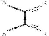
(a)                         (b)      

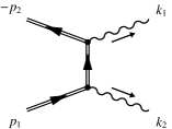
Figure 1: The leading-order Feynman diagrams for electron-positron annihilation into two photons in a plane-wave field: (a) the direct diagram, and (b) the exchange diagram. Double lines represent dressed (Volkov) wave functions and propagators (see the main text for details).

II Formalism

The formalism, that we employ, combines light-cone quantization Bjorken et al. (1971); Mustaki et al. (1991); Brodsky et al. (1998); Burkardt (2002) and Furry picture Furry (1951); Fradkin et al. (1991) (a detailed discussion of the formalism utilized here is provided in Ref. Bragin (2019)). With the quantization on the light cone, a plane-wave background and particularly momentum conservation laws are naturally included into the calculations (see Refs. Dinu and Torgrimsson (2018, 2019) for an application of light-cone quantization to trident and double Compton scattering). Also, the light-cone representation of the electromagnetic interaction via three types of vertices (see Appendix A), or, equivalently, the representation of the electron propagator (and also of the photon one) as combination of noninstantaneous and instantaneous terms (this can be done within the instant-form quantization as well Kogut and Soper (1970); Mantovani et al. (2016); see also Refs. Seipt and Kämpfer (2012); Mackenroth and Di Piazza (2013); Hartin (2016)) allows one to write the spinor prefactors via fermion dressed momenta (see below), and, as a consequence, the final expressions formally have no explicit dependence on the background field and asymptotic fermion momenta. In this respect, the obtained result is similar to the ones usually derived in vacuum, where the final expressions depend on the particle four-momenta in the form of Mandelstam variables Berestetskii et al. (1982).

The laser field is described classically by the field tensor $F^{\mu\nu}(\phi)$, which is a function of the scalar product $\phi=k_{0}x$, with $k_{0}^{\mu}$ being the characteristic wave four-vector of the field or, in the quantum language, the characteristic four-momentum of a laser photon ($k_{0}^{2}=k_{0}^{\mu}k_{0\mu}=0$) and $x^{\mu}$ being a position four-vector. We assume that $F^{\mu\nu}(\phi)$ does not contain a zero-frequency contribution, i.e., the integral of $F^{\mu\nu}(\phi)$ over the whole real axis vanishes. Then the most general form of $F^{\mu\nu}(\phi)$ is given by

$$F^{\mu\nu}(\phi)=\sum_{i=1,2}f_{i}^{\mu\nu}\psi_{i}^{\prime}(\phi),$$ (1)

where $f_{i}^{\mu\nu}=k_{0}^{\mu}a_{i}^{\nu}-k_{0}^{\nu}a_{i}^{\mu}$, the four-vectors $a_{i}^{\mu}$ define the amplitude of the field in two polarization directions ($k_{0}a_{i}=0$, $a_{1}a_{2}=0$), and the functions $\psi_{i}^{\prime}(\phi)=\mathrm{d}\psi_{i}(\phi)/\mathrm{d}\phi$ characterize its shape [$|\psi_{i}^{\prime}(\phi)|\lesssim 1$]. In the following, each of the indices $i,j$ always take the values 1, 2.

For an arbitrary four-vector $a^{\mu}$, we define light-cone coordinates as $a^{+}=a\eta$, $a^{-}=a\bar{\eta}$, and $a^{i}=-ae_{i}$ [$\boldsymbol{a}^{\perp}=(a^{1},a^{2})$], where $\{\eta^{\mu},\bar{\eta}^{\mu},e_{1}^{\mu},e_{2}^{\mu}\}$ is a light-cone basis (see Appendix A for details). Below, we employ the canonical light-cone basis, which is given by Meuren (2015)

$$\eta^{\mu}=\frac{k_{0}^{\mu}}{m},\quad\bar{\eta}^{\mu}=\frac{P^{\mu}}{P^{+}}-\frac{P^{2}\eta^{\mu}}{2P^{+2}},\quad e_{1}^{\mu}=\frac{P_{\lambda}f_{1}^{\lambda\mu}}{mP^{+}\sqrt{-a_{1}^{2}}},\quad e_{2}^{\mu}=\frac{P_{\lambda}f_{2}^{\lambda\mu}}{mP^{+}\sqrt{-a_{2}^{2}}},$$ (2)

where the four-vector $P^{\mu}$ is arbitrary except that $P^{+}\neq 0$. The calculations are greatly simplified if one chooses

$$P^{\mu}=p_{1}^{\mu}+p_{2}^{\mu},$$ (3)

which implies $\boldsymbol{p}_{2}^{\perp}+\boldsymbol{p}_{1}^{\perp}=\boldsymbol{k}_{2}^{\perp}+\boldsymbol{k}_{1}^{\perp}=\boldsymbol{0}$ [see Eq. (2) and Appendix A; also note that $f_{i}^{\mu\nu}$ is an antisymmetric tensor]. Here, $p_{1}^{\mu}$ and $p_{2}^{\mu}$ are the asymptotic four-momenta of the incoming electron and positron outside the plane wave, respectively, whereas $k_{1}^{\mu}$ and $k_{2}^{\mu}$ are the four-momenta of the final photons (see Fig. 1 and note that in the following we employ wave packets for the electron and positron, and therefore $p_{1}^{\mu}$ and $p_{2}^{\mu}$ will be ultimately identified with the central four-momenta).

Since $\eta^{\mu}=k_{0}^{\mu}/m$, the laser phase is $\phi=mx^{+}$ and the field $F^{\mu\nu}(\phi)$ depends only on the light-cone time. With the adoption of the light-cone gauge $A^{+}(x)=0$, the four-vector potential for $F^{\mu\nu}(\phi)$ reads

$$A^{\mu}(\phi)=\sum_{i}a_{i}^{\mu}\psi_{i}(\phi).$$ (4)

In the following, we assume $A^{\mu}(-\infty)=0$, which implies $\psi_{i}(-\infty)=0$ [together with the fact of the absence of a zero-frequency contribution in $F^{\mu\nu}(\phi)$ this implies that also $A^{\mu}(\infty)=0$, and therefore $\psi_{i}(\infty)=0$].

The solution of the Dirac equation with the classical field (4) is the Volkov solution Volkov (1935). We write the positive-energy one in the form Hartin (2016)

$$\psi_{p\sigma}(x)=K_{p}(\phi)\frac{u_{p\sigma}}{\sqrt{2p^{+}}}\mathrm{e}^{iS_{p}(x)},$$ (5)

with

$$K_{p}(\phi)=[\gamma\pi_{p}(\phi)+m]\frac{\gamma^{+}}{2p^{+}},\quad S_{p}(x)=-px-\mathcal{S}_{p}(\phi),\quad\mathcal{S}_{p}(\phi)=\int\displaylimits_{-\infty}^{\phi}\mathrm{d}\beta\,\left(\frac{epA(\beta)}{mp^{+}}-\frac{e^{2}A^{2}(\beta)}{2mp^{+}}\right),$$ (6)

and the negative-energy one in an analogous way (see Appendix A). Note that the phase $S_{p}(x)$ is the classical action of an electron in the plane wave and that the dressed four-momentum $\pi_{p}^{\mu}(\phi)=-\partial^{\mu}S_{p}(x)-eA^{\mu}(\phi)$ is the corresponding solution of the Lorentz equation. It is given by

$$\pi_{p}^{\mu}(\phi)=p^{\mu}-eA^{\mu}(\phi)+\eta^{\mu}\left(\frac{epA(\phi)}{p^{+}}-\frac{e^{2}A^{2}(\phi)}{2p^{+}}\right),$$ (7)

such that $\pi_{p}^{2}(\phi)=p^{2}$, $\pi_{p}^{+}(\phi)=p^{+}$. The free Dirac bispinor $u_{p\sigma}$ is normalized such that $\bar{u}_{p\sigma}u_{p\sigma^{\prime}}=2m\delta_{\sigma\sigma^{\prime}}$, $\bar{u}_{p\sigma}\gamma^{\mu}u_{p\sigma^{\prime}}=2p^{\mu}\delta_{\sigma\sigma^{\prime}}$, $\sum_{\sigma}u_{p\sigma}\bar{u}_{p\sigma}=\gamma p+m$, where $\bar{u}_{p\sigma}=u_{p\sigma}^{\dagger}\gamma^{0}$ and the dagger denotes the Hermitian conjugate, and analogous expressions are valid for the negative-energy bispinor $v_{p\sigma}$ Berestetskii et al. (1982).

The fermion field $\psi(x)$ is expanded in the basis set of the Volkov wave functions (5) (and analogous ones for negative-energy states) and, as a consequence, in all diagrams free fermion lines are replaced with the corresponding Volkov ones Furry (1951); Fradkin et al. (1991) (details on the quantization are given in Appendix A).

Though in electrodynamics, quantized on the light cone, there are three types of vertices, for our purposes it is convenient to combine them in the form of propagators. Then we have only the usual three-point QED vertex, but each electron and photon Feynman propagator consists of two terms Kogut and Soper (1970); Mantovani et al. (2016) (see also Refs. Seipt and Kämpfer (2012); Mackenroth and Di Piazza (2013); Hartin (2016)), in particular, for the electron propagator $G(x_{2},x_{1})$ we have $G(x_{2},x_{1})=G^{\text{(ni)}}(x_{2},x_{1})+G^{\text{(in)}}(x_{2},x_{1})$, with $G^{\text{(ni)}}(x_{2},x_{1})$ being a noninstantaneous (propagating) part,

$$G^{(\text{ni})}(x_{2},x_{1})=\int\frac{\mathrm{d}^{4}p}{(2\pi)^{4}}\mathrm{e}^{-ip(x_{2}-x_{1})-i\mathcal{S}_{p}(\phi_{2},\phi_{1})}K_{p}(\phi_{2})\frac{\gamma\tilde{p}+m}{p^{2}-m^{2}+i\epsilon}\bar{K}_{p}(\phi_{1}),$$ (8)

where $\bar{K}_{p}(\phi)=\gamma^{0}K_{p}^{\dagger}(\phi)\gamma^{0}$, and with $G^{\text{(in)}}(x_{2},x_{1})$ being an instantaneous part,

$$G^{(\text{in})}(x_{2},x_{1})=\int\frac{\mathrm{d}^{4}p}{(2\pi)^{4}}\mathrm{e}^{-ip(x_{2}-x_{1})-i\mathcal{S}_{p}(\phi_{2},\phi_{1})}\frac{\gamma^{+}}{2p^{+}}.$$ (9)

Here, $\mathcal{S}_{p}(\phi_{2},\phi_{1})=\mathcal{S}_{p}(\phi_{2})-\mathcal{S}_{p}(\phi_{1})$ and

$$\tilde{p}^{\mu}=\left(p^{+},\frac{\boldsymbol{p}^{\perp 2}+m^{2}}{2p^{+}},\boldsymbol{p}^{\perp}\right),$$ (10)

such that $\tilde{p}^{2}=m^{2}$.

Below, we will employ the classical intensity parameters Ritus (1985); Di Piazza et al. (2012)

$$\xi_{i}=\frac{|e|\sqrt{-a_{i}^{2}}}{m},$$ (11)

and we also introduce $\xi=\sqrt{\xi_{1}^{2}+\xi_{2}^{2}}$. Other parameters characterizing the scattering process are the quantum nonlinearity parameters, which are defined as $\chi_{i}=p_{i}^{+}\xi/m$ for the fermions, and analogously for the photons Ritus (1985); Di Piazza et al. (2012). Note that by considering the interaction with the quantized photon field to leading order, we implicitly assume that the quantum nonlinearity parameters are much smaller than $1/\alpha^{3/2}\approx 1600$, such that this interaction can be treated perturbatively. This assumption is reasonable for current and near-future laser-based setups (for discussions of the fully nonperturbative regime, see, e.g., Refs. Fedotov (2017); Yakimenko et al. (2019); Podszus and Di Piazza (2019); Ilderton (2019); Baumann et al. (2019); Di Piazza et al. (2020)).

For a process with two incoming particles, the classical intensity parameters and the quantum nonlinearity parameters do not exhaust the list of quantities, that are necessary for describing the scattering (even when considering an observable obtained by averaging/summing over the discrete quantum numbers and by integrating over the final momenta). We introduce the additional parameters $t_{i}(\phi)$, which are given by Bragin (2019)

$$t_{i}(\phi)=\frac{|e|\pi_{e,p_{1}}^{\mu}(\phi)f_{i\mu\nu}\pi_{-e,p_{2}}^{\nu}(\phi)}{\xi_{i}m^{3}(p_{1}^{+}+p_{2}^{+})},$$ (12)

where $\pi_{e,p_{1}}^{\mu}(\phi)=\pi_{p_{1}}^{\mu}(\phi)$ and $\pi_{-e,p_{2}}^{\mu}(\phi)=-\pi_{-p_{2}}^{\mu}(\phi)$ are the dressed four-momenta of the electron and the positron, respectively. The asymptotic values of $t_{i}(\phi)$ are denoted as $t_{i}$, they have been employed in the literature before Ritus (1985).

The parameters $t_{i}(\phi)$ have a particularly clear physical interpretation if we use the canonical light-cone basis (2) with $P^{\mu}$ from Eq. (3). With this choice, we have $\boldsymbol{\pi}_{e,p_{1}}^{\perp}(\phi)+\boldsymbol{\pi}_{-e,p_{2}}^{\perp}(\phi)=\boldsymbol{p}_{1}^{\perp}+\boldsymbol{p}_{2}^{\perp}=\boldsymbol{0}$ and $t_{i}(\phi)=\pi_{p_{1}}^{i}(\phi)/m$, i.e., $t_{1}(\phi)$ and $t_{2}(\phi)$ correspond to the transverse dressed momentum components of the incoming particles (with respect to the laser-pulse propagation direction).

III Cross section

As has been mentioned in the Introduction, the result of a collision of an electron, a positron, and a finite-duration laser pulse depends on the existence of a collision region and the time of arrival of each participant at this region. Thus, in the most general setup, one cannot rely on the description of the incoming particles via monochromatic plane waves, since they have an infinite temporal and spatial extent.

Therefore, in order to consistently describe the reaction $e^{-}e^{+}\Rightarrow\gamma\gamma$, we represent the electron and the positron as normalized wave packets with central on-shell four-momenta $p_{1}^{\mu}$ and $p_{2}^{\mu}$, respectively. A positive-energy wave packet $\Psi_{p}(x)$ with the central four-momentum $p^{\mu}$ is constructed according to

$$\Psi_{p}(x)=\int\frac{\tilde{\mathrm{d}}^{3}q}{(2\pi)^{3}}\tilde{f}_{p}(q)\psi_{q}(x),$$ (13)

where $\tilde{f}_{p}(q)$ is the momentum distribution density and $\psi_{q}(x)$ is the positive-energy Volkov state (5) with four-momentum $q^{\mu}$ (for the definition of $\tilde{\mathrm{d}}^{3}q$ see Appendix A). Note that Volkov states are on-shell such that $q^{-}=(\boldsymbol{q}^{\perp 2}+m^{2})/(2q^{+})$, i.e., $\tilde{f}_{p}(q)$ depends on $\boldsymbol{q}^{\perp}$ and $q^{+}$ only, but for simplicity, we write $\tilde{f}_{p}(q)$ as a function of $q^{\mu}$. The fact that the function $\tilde{f}_{p}(q)$ is centered around the on-shell four-momentum $p^{\mu}$ has to be intended analogously. Correspondingly, one can also define negative-energy wave packets. We refer to Appendix B for further details about the general properties of the wave packets $\Psi_{p}(x)$.

The polarization degrees of freedom of both incoming (outgoing) particles are averaged (summed) in the final expressions, with the assumption of the initial states being unpolarized, and therefore, for notational brevity, we suppress the subscripts for these degrees of freedom.

As already mentioned, the final photon four-momenta are $k_{1}^{\mu}$ and $k_{2}^{\mu}$ ($k^{2}_{1}=k^{2}_{2}=0$). The $S$-matrix element corresponding to the diagrams in Fig. 1 can be written as

$$S_{fi}=i\int\frac{\tilde{\mathrm{d}}^{3}q_{2}}{(2\pi)^{3}}\frac{\tilde{\mathrm{d}}^{3}q_{1}}{(2\pi)^{3}}\tilde{f}_{2}^{*}(q_{2})\tilde{f}_{1}(q_{1})\int\mathrm{d}^{4}x_{2}\mathrm{d}^{4}x_{1}\,\tilde{T}(x_{2},x_{1},q_{2},q_{1}),$$ (14)

where we have introduced the shorthand notation $\tilde{f}_{1}(q)=\tilde{f}_{p_{1}}(q)$ and $\tilde{f}_{2}^{*}(q)=\tilde{f^{\prime}}_{p_{2}}^{*}(q)$ for the electron and positron wave-packet momentum distributions $\tilde{f}_{p_{1}}(q)$ and $\tilde{f^{\prime}}_{p_{2}}^{*}(q)$, respectively (an asterisk indicates the complex conjugate), and

$$\tilde{T}(x_{2},x_{1},q_{2},q_{1})=\int\frac{\mathrm{d}^{4}p_{3}}{(2\pi)^{4}}\frac{M^{\text{direct}}(\phi_{2},\phi_{1},q_{2},q_{1})}{4\sqrt{k_{2}^{+}k_{1}^{+}q_{2}^{+}q_{1}^{+}}}\exp[ i(k_{2}-p_{3}-q_{2})x_{2}+i(k_{1}+p_{3}-q_{1})x_{1}$$

$$-i\mathcal{S}_{p_{3}}(\phi_{2},\phi_{1})-i\mathcal{S}_{q_{1}}(\phi_{1})+i\mathcal{S}_{-q_{2}}(\phi_{2})]$$

$$+\{\gamma_{1}\leftrightarrow\gamma_{2}\},$$ (15)

with

$$M^{\text{direct}}(\phi_{2},\phi_{1},q_{2},q_{1})= -e^{2}\bar{v}_{q_{2}}\left[K_{-q_{2}p_{3}}^{\mu}(\phi_{2})\frac{\gamma\tilde{p}_{3}+m}{p_{3}^{2}-m^{2}+i\epsilon}K_{p_{3}q_{1}}^{\nu}(\phi_{1})\right]u_{q_{1}}\epsilon_{2\mu}^{*}\epsilon_{1\nu}^{*}$$

$$-e^{2}\bar{v}_{q_{2}}\left[\frac{K_{-q_{2}q_{1}}^{\mu\nu}(\phi_{2},\phi_{1})}{2p_{3}^{+}}\right]u_{q_{1}}\epsilon_{2\mu}^{*}\epsilon_{1\nu}^{*}.$$ (16)

Here and below, $\phi_{i}=k_{0}x_{i}=mx_{i}^{+}$ and the term $\{\gamma_{1}\leftrightarrow\gamma_{2}\}$ corresponds to the exchange diagram with the photon quantum numbers swapped (see Fig. 1b). Also, the functions $K_{pp^{\prime}}^{\mu}(\phi)$ and $K_{pp^{\prime}}^{\mu\nu}(\phi,\phi^{\prime})$ are given by

$$K_{pp^{\prime}}^{\mu}(\phi)=\bar{K}_{p}(\phi)\gamma^{\mu}K_{p^{\prime}}(\phi),\quad K_{pp^{\prime}}^{\mu\nu}(\phi,\phi^{\prime})=\bar{K}_{p}(\phi)\gamma^{\mu}\gamma^{+}\gamma^{\nu}K_{p^{\prime}}(\phi^{\prime}).$$ (17)

In the following and analogously to the vacuum case (see, e.g., Refs. Goldberger and Watson (1964); Itzykson and Zuber (1980)), we assume the momentum distributions of the electron and the positron being sufficiently narrowly peaked around the central four-momenta and the detectors not being sensitive enough to resolve the final momenta within the widths of such distributions, such that we can in particular replace the four-momenta $q_{i}^{\mu}$ with the central ones in relatively slowly varying functions, i.e.,

$$M^{\text{direct}}(\phi_{2},\phi_{1},q_{2},q_{1})/\sqrt{q_{2}^{+}q_{1}^{+}}\approx M^{\text{direct}}(\phi_{2},\phi_{1})/\sqrt{p_{2}^{+}p_{1}^{+}},$$ (18)

where $M^{\text{direct}}(\phi_{2},\phi_{1})=M^{\text{direct}}(\phi_{2},\phi_{1},p_{2},p_{1})$, and we do the same for the exchange term as well.

The total probability, obtained as the modulus squared of Eq. (14), averaged over the initial polarization states and summed over all final polarization and momentum states, can be written as

$$W \approx\frac{1}{4}\sum_{\text{qn}}\left|\int\mathrm{d}^{4}x_{2}\mathrm{d}^{4}x_{1}F_{2}^{*}(x_{2})F_{1}(x_{1})\tilde{T}(x_{2},x_{1},p_{2},p_{1})\right|^{2}$$

$$=\frac{1}{4}\sum_{\text{qn}}\int\mathrm{d}^{4}x_{2}\mathrm{d}^{4}x_{1}\mathrm{d}^{4}x^{\prime}_{2}\mathrm{d}^{4}x^{\prime}_{1}F_{2}^{*}(x_{2})F_{2}(x^{\prime}_{2})F_{1}(x_{1})F_{1}^{*}(x^{\prime}_{1})\tilde{T}(x_{2},x_{1},p_{2},p_{1})\tilde{T}^{*}(x^{\prime}_{2},x^{\prime}_{1},p_{2},p_{1}),$$ (19)

where the abbreviation “qn” indicates that the sum/integral is taken over the discrete quantum numbers of the initial and final particles and the momenta of the final photons. Also, in Eq. (III) we have introduced the electron and positron wave-packet amplitudes $F_{1}(x_{1})$ and $F_{2}^{*}(x_{2})$ in configuration space, which are defined analogously to the vacuum case Goldberger and Watson (1964), e.g., for an electron we have

$$F_{p}(x)=\int\frac{\tilde{\mathrm{d}}^{3}q}{(2\pi)^{3}}\tilde{f}_{p}(q)\exp[-i(q-p)x-i\mathcal{S}_{q}(\phi)+i\mathcal{S}_{p}(\phi)]$$ (20)

for a given momentum distribution $\tilde{f}_{p}(q)$. The scalar wave packet in configuration space is given by

$$f_{p}(x)=\int\frac{\tilde{\mathrm{d}}^{3}q}{(2\pi)^{3}}\tilde{f}_{p}(q)\exp[-iqx-i\mathcal{S}_{q}(\phi)]=F_{p}(x)\exp[-ipx-i\mathcal{S}_{p}(\phi)]$$ (21)

(for a positron, the expressions are analogous). Note that $|f_{p}(x)|^{2}=|F_{p}(x)|^{2}$ is the (time-dependent) particle density. The properties of the particle density $|F_{p}(x)|^{2}$ are discussed in Appendix B, and we only recall here that for a narrow wave packet, under the condition that also $|f_{p}(x)|^{2}$ is sufficiently peaked in configuration space, the center of the distribution $|f_{p}(x)|^{2}$ follows the classical trajectory of an electron in a given plane wave (see Appendix B for further details).

In principle, Eq. (III) is the expression one needs to employ in order to evaluate the total probability of the process under consideration. However, depending on the widths of the wave packets and on the formation lengths of the integrals in the space-time variables, one can achieve further simplifications.

The first step is to assume that the wave packets are sufficiently narrow (in momentum space), that on the formation length of a single-vertex process (essentially, a process obtained by cutting the propagator line, see Fig. 1) one can neglect the interference among the wave packets, i.e.,

$$F_{1}(x_{1})F_{1}^{*}(x^{\prime}_{1})=F_{1}(X_{1}-\delta_{1}/2)F_{1}^{*}(X_{1}+\delta_{1}/2)\approx|f_{1}(X_{1})|^{2}$$ (22)

and analogously for the positron wave-packet amplitudes, where

$$X_{i}^{\mu}=(x_{i}^{\mu}+x_{i}^{\prime\mu})/2,\quad\delta_{1}^{\mu}={x_{1}^{\prime}}^{\mu}-x_{1}^{\mu},\quad\delta_{2}^{\mu}=x_{2}^{\mu}-{x_{2}^{\prime}}^{\mu}.$$ (23)

Note that the approximation (22) is not assumed to be valid for all values of $\delta_{1}^{\mu}$. It is assumed to be valid for $\delta_{1}^{\mu}$ only within the formation region of the integral in this variable, i.e., within an effective part of the whole space which mostly contributes to the value of the integral.

We also point out that the assertion in Eq. (22) [and the corresponding one for $F_{2}(x_{2}^{\prime})F_{2}^{*}(x_{2})$] is a more complicated statement than in vacuum, in the sense that the typical scale of $\delta_{1}^{\mu}$ (and of $\delta_{2}^{\mu}$ for the positron) depends in general on the form and on the intensity of a considered background field, and Eq. (22) results from an interplay between the scale introduced by the field and the scale of the wave packets (details are given in Appendix C).

Under the approximation (22) and an analogous one for the positron, the total probability (III) reads

$$W\approx\int\mathrm{d}^{4}X_{2}\mathrm{d}^{4}X_{1}\,|f_{2}(X_{2})|^{2}|f_{1}(X_{1})|^{2}W(X_{2},X_{1}),$$ (24)

with the two-point probability distribution

$$W(X_{2},X_{1})=\frac{1}{4}\sum_{\text{qn}}\int\mathrm{d}^{4}\delta_{2}\mathrm{d}^{4}\delta_{1}\,\tilde{T}(x_{2},x_{1},p_{2},p_{1})\tilde{T}^{*}(x^{\prime}_{2},x^{\prime}_{1},p_{2},p_{1}).$$ (25)

An additional simplification is attained under the assumption, that on a typical distance between $X_{1}^{\mu}$ and $X_{2}^{\mu}$ (in essence, on the typical distance between the two single-vertex processes, see Fig. 1) the wave packets do not change significantly, i.e.,

$$|f_{2}(X_{2})|^{2}|f_{1}(X_{1})|^{2}=|f_{2}(x+\delta/2)|^{2}|f_{1}(x-\delta/2)|^{2}\approx|f_{2}(x)|^{2}|f_{1}(x)|^{2},$$ (26)

where

$$x^{\mu}=(X_{2}^{\mu}+X_{1}^{\mu})/2,\quad\delta^{\mu}=X_{2}^{\mu}-X_{1}^{\mu}.$$ (27)

Then Eq. (24) transforms into

$$W\approx\int\mathrm{d}^{4}x\,|f_{2}(x)|^{2}|f_{1}(x)|^{2}W(x),$$ (28)

where

$$W(x)=W(\phi)=\frac{1}{4}\sum_{\text{qn}}\int\mathrm{d}^{4}\delta\mathrm{d}^{4}\delta_{2}\mathrm{d}^{4}\delta_{1}\,\tilde{T}(x_{2},x_{1},p_{2},p_{1})\tilde{T}^{*}(x^{\prime}_{2},x^{\prime}_{1},p_{2},p_{1}).$$ (29)

Equation (28) is the approximation that is commonly used for the description of scattering in vacuum and that allows us to define a cross section, a quantity, which characterizes the process itself without relying on the precise shape of the wave packets Goldberger and Watson (1964); Itzykson and Zuber (1980). We stress that in a background field the assumption (26) can be restrictive as the intermediate particle may become real, and hence $\delta^{\mu}$ can have a macroscopic scale, i.e., of the order of the extension of the background field. For the highly nonlinear regime ($\xi\gg 1$), semiquantitative estimations imply (see Appendix C for details) that if one excludes the contribution of the case of the intermediate particle being real, both approximations (22) and (26) are valid as soon as the relations $|\Delta\boldsymbol{p}_{1}^{\perp}|\ll\max(m,|\boldsymbol{\pi}_{p_{1}}^{\perp}(\phi)|)$, $\Delta p_{1}^{+}\ll p_{1}^{+}$ for the electron wave packet and analogous ones for the positron wave packet are fulfilled ($\Delta p_{1}^{+}$ and $\Delta\boldsymbol{p}_{1}^{\perp}$ are the corresponding wave-packet widths).

Now, it is worth pointing out an additional difference with the vacuum case. In the latter case, in fact, the quantity $W(x)$ is independent of the coordinates and therefore non-negative Goldberger and Watson (1964); Itzykson and Zuber (1980). In contrast to this, the quantity $W(\phi)$ here explicitly depends on the light-cone time (via $\phi$) and it can be negative for some values of $\phi$. Thus, generally speaking, the quantity

$$w(x)=|f_{2}(x)|^{2}|f_{1}(x)|^{2}W(\phi)$$ (30)

cannot be interpreted as a probability per unit time and unit volume. However, it can be seen as a quantity, which generalizes this probability and which entails interference effects among contributions from different points of the particles trajectory in the plane wave, and therefore may become negative. This is somewhat similar to the relation between a classical phase-space distribution and the Wigner distribution, with the latter generalizing the former and, indeed, being also potentially negative Wigner (1932).

Furthermore, we can define a generalized (local) cross section, which, though not being directly an observable quantity, since it can become negative, is a useful theoretical tool for investigating the influence of the external field on the scattering process. We follow the approach in the instant-form quantization in vacuum, where the cross section is obtained from the probability per unit time and unit volume by dividing it by the factor $|g_{2}(x)|^{2}|g_{1}(x)|^{2}I/(p_{2}^{0}p_{1}^{0})$, where $I=\sqrt{(p_{2}p_{1})^{2}-m^{4}}$ and $g_{i}(x)$ are wave packets in the instant form Itzykson and Zuber (1980); Berestetskii et al. (1982). Then in our case we can analogously introduce the local cross section as

$$\sigma(\phi)=\frac{p_{2}^{+}p_{1}^{+}}{|f_{2}(x)|^{2}|f_{1}(x)|^{2}I(\phi)}w(x)=\frac{p_{2}^{+}p_{1}^{+}}{I(\phi)}W(\phi),$$ (31)

where the invariant $I(\phi)$ reads

$$I(\phi)=\sqrt{[\pi_{-e,p_{2}}(\phi)\pi_{e,p_{1}}(\phi)]^{2}-m^{4}}.$$ (32)

Below, we explicitly verify (except for the interference term, as has been pointed out in the Introduction) that in the absence of the background field the cross section (31) reduces to the one, known for the vacuum case in the instant-form quantization. One should also keep in mind that the choice of the invariant $I(\phi)$ implies that the cross section is normalized to the flux coming into the point $x^{\mu}$ inside the laser field and in this sense is a local quantity. This can be useful, for instance, in the analysis of the importance of the studied process in the development of QED cascades where the colliding particles are produced inside the field. However, if one would like to consider a beam-beam collision experiment in the presence of a laser field, then the use of the vacuum counterpart $I$ in place of $I(\phi)$ could be more convenient. The total probability $W$ is of course independent of this choice.

We emphasize that Eqs. (24) and (28) are not ensured to provide a positive result in a general case, i.e., without taking into account the validity of the approximations (22) and (26), and that one has to ultimately rely on the probability $W$ in Eq. (III), if these approximations break down.

With the use of Eqs. (III) and (III), we obtain for the cross section:

$$\sigma(\phi)=\int\displaylimits_{0}^{p_{2}^{+}+p_{1}^{+}}\frac{\mathrm{d}k_{1}^{+}}{2\pi}\int\frac{\mathrm{d}^{2}k_{1}^{\perp}}{(2\pi)^{2}}\frac{1}{32k_{2}^{+}k_{1}^{+}I(\phi)}\int\mathrm{d}\delta^{+}\mathrm{d}\delta_{2}^{+}\mathrm{d}\delta_{1}^{+}\,\frac{1}{4}\sum\displaylimits_{\sigma_{i},\lambda_{i}}\tilde{M}(\phi_{2},\phi_{1},p_{2},p_{1})\tilde{M}^{*}(\phi_{2}^{\prime},\phi_{1}^{\prime},p_{2},p_{1}),$$ (33)

where $k_{2}^{(+,\perp)}=(p_{2}+p_{1}-k_{1})^{(+,\perp)}$, $\sigma_{i}$ and $\lambda_{i}$ denote the polarization states of the incoming and outgoing particles, respectively, and we have divided the result by 2, in order to compensate for the double counting of the final states of the two identical particles. The reduced matrix element $\tilde{M}(\phi_{2},\phi_{1},p_{2},p_{1})$ is given by

$$\tilde{M}(\phi_{2},\phi_{1},p_{2},p_{1})=\int\frac{\mathrm{d}p_{3}^{-}}{2\pi}M^{\text{direct}}(\phi_{2},\phi_{1})\exp[ i(k_{2}^{-}-p_{3}^{-}-p_{2}^{-})x_{2}^{+}+i(k_{1}^{-}+p_{3}^{-}-p_{1}^{-})x_{1}^{+}$$

$$-i\mathcal{S}_{p_{3}}(\phi_{2},\phi_{1})-i\mathcal{S}_{p_{1}}(\phi_{1})+i\mathcal{S}_{-p_{2}}(\phi_{2})]$$

$$+\{\gamma_{1}\leftrightarrow\gamma_{2}\},$$ (34)

where $p_{3}^{(+,\perp)}=(p_{1}-k_{1})^{(+,\perp)}=(k_{2}-p_{2})^{(+,\perp)}$.

The quantity $\tilde{M}(\phi_{2},\phi_{1},p_{2},p_{1})$ in Eq. (III) contains four distinct terms because $M^{\text{direct}}(\phi_{2},\phi_{1})$ alone consists of a noninstantaneous and an instantaneous contributions, corresponding to the first and to the second term on the right-hand side of Eq. (III), respectively. Taking the modulus squared yields 16 terms. However, only eight of them are different after we sum over the states of the final photons, i.e.,

$$\sigma(\phi)=\sigma^{\text{dd}}(\phi)+\sigma^{\text{ee}}(\phi)+\sigma^{\text{de}}(\phi)+\sigma^{\text{ed}}(\phi)=2\sigma^{\text{dd}}(\phi)+2\sigma^{\text{de}}(\phi),$$ (35)

where $\sigma^{\text{dd}}(\phi)$ is the contribution, arising from squaring the amplitude for the direct diagram (see Fig. 1a), and can be written as

$$\sigma^{\text{dd}}(\phi)=\sigma^{\text{nndd}}(\phi)+\sigma^{\text{nidd}}(\phi)+\sigma^{\text{indd}}(\phi)+\sigma^{\text{iidd}}(\phi).$$ (36)

The four contributions in Eq. (36) are obtained via squaring corresponding parts of the amplitude [$\sigma^{\text{nndd}}(\phi)$ originates from squaring the noninstantaneous direct term, $\sigma^{\text{nidd}}(\phi)$ from the product of the noninstantaneous and complex-conjugate instantaneous direct terms, etc.], with subsequent rearrangements, as described below and in Appendix D. The other contributions in Eq. (35) can be written down analogously. In the following, we only consider $\sigma^{\text{dd}}(\phi)$. We note that for the differential quantities the interference terms “de” and “ed” lead to an enhancement of the cross section by a factor of 2 in the case of the final photons being in the same state. On the other hand, at least in an ultrarelativistic setup, the available phase space is typically so large that one might expect that the integrated interference term $\sigma^{\text{de}}(\phi)$ should give a negligible contribution. Indeed, e.g., in the vacuum case, the interference contribution for the total cross section is relatively large only for mildly relativistic collisions Berestetskii et al. (1982). If we assume a similar behavior in our case, then we should expect that the term $\sigma^{\text{de}}(\phi)$ might be nonnegligible only for some $\sqrt{s(\phi)}\sim m$, where the invariant mass squared $s(\phi)$ in the field is defined as

$$s(\phi)=[\pi_{-e,p_{2}}(\phi)+\pi_{e,p_{1}}(\phi)]^{2}=\frac{m^{2}(p_{2}^{+}+p_{1}^{+})^{2}}{p_{2}^{+}p_{1}^{+}}[1+\boldsymbol{t}^{\perp 2}(\phi)],$$ (37)

with $\boldsymbol{t}^{\perp 2}(\phi)=t_{1}^{2}(\phi)+t_{2}^{2}(\phi)$. It follows that if $p_{1}^{+}\sim p_{2}^{+}$ and $\boldsymbol{t}^{\perp 2}(\phi)\lesssim 1$, the interference term might provide a somewhat sizable contribution. However, for the phase average $\langle t_{i}^{2}(\phi)\rangle$ we have $\langle t_{i}^{2}(\phi)\rangle\approx t_{i}^{2}+\xi_{i}^{2}\langle\psi_{i}^{2}(\phi)\rangle\gg 1$ if $\xi_{i}\gg 1$ [we assume that $\langle\psi_{i}(\phi)\rangle\ll 1$]. This implies that in the highly nonlinear regime, i.e., in the regime of $\xi\gg 1$, and for sufficiently long laser pulses, common values of $|\boldsymbol{t}^{\perp}(\phi)|$ are much larger than unity. Therefore, if one considers dynamics over several laser periods, one might expect that on average the term $\sigma^{\text{de}}(\phi)$ can be neglected.

Summing over the final photon polarizations results in the replacement

$$\epsilon^{\mu}_{i}\epsilon^{*\nu}_{i}\to-g^{\mu\nu}$$ (38)

(we discard the terms proportional to $k_{i}^{\mu}$ and $k_{i}^{\nu}$ due to the Ward identity).

Averaging over the polarization states of the initial particles results in the replacements Berestetskii et al. (1982)

$$u_{p_{1}}\bar{u}_{p_{1}}\to\rho_{p_{1}},\quad v_{p_{2}}\bar{v}_{p_{2}}\to\rho^{(-)}_{p_{2}},$$ (39)

and taking the trace over the bispinor part of $\tilde{M}(\phi_{2},\phi_{1},p_{2},p_{1})\tilde{M}^{*}(\phi_{2}^{\prime},\phi_{1}^{\prime},p_{2},p_{1})$. The quantities $\rho_{p_{1}}$ and $\rho^{(-)}_{p_{2}}$ denote the electron and positron density matrices, respectively. In the case of the initial particles being unpolarized, we have

$$\rho_{p_{1}}=\frac{1}{2}(\gamma p_{1}+m),\quad\rho^{(-)}_{p_{2}}=-\rho_{-p_{2}}=\frac{1}{2}(\gamma p_{2}-m).$$ (40)

Upon squaring the noninstantaneous part of the direct diagram, we obtain

$$\frac{1}{4}\sum_{\sigma_{i},\lambda_{i}}\tilde{M}^{\text{nd}}\tilde{M}^{\text{nd}*}=-8e^{4}m^{4}\int\frac{\mathrm{d}p_{3}^{-}}{2\pi}\frac{\mathrm{d}{p_{3}^{\prime}}^{-}}{2\pi}\exp\left(i\Phi^{\text{dd}}\right)\frac{\mathcal{M}^{\text{nndd}}}{(p_{3}^{2}-m^{2}+i\epsilon)({p_{3}^{\prime}}^{2}-m^{2}-i\epsilon)},$$ (41)

with ${p_{3}^{\prime}}^{(+,\perp)}=p_{3}^{(+,\perp)}$. The phase $\Phi^{\text{dd}}$ reads

$$\Phi^{\text{dd}}=(k_{2}^{-}-p_{2}^{-})\delta_{2}^{+}-(k_{1}^{-}-p_{1}^{-})\delta_{1}^{+}-p_{3}^{-}(x_{2}^{+}-x_{1}^{+})+{p_{3}^{\prime}}^{-}(x_{2}^{\prime+}-x_{1}^{\prime+})+\Phi_{F}^{\text{dd}},$$ (42)

with the field-dependent part $\Phi_{F}^{\text{dd}}$ given by [we use the canonical light-cone basis (2) with $P^{\mu}$ from Eq. (3)]

$$\Phi_{F}^{\text{dd}}=\phantom{-}\frac{m}{p_{3}^{+}}\sum\displaylimits_{i}\xi_{i}k_{1}^{i}\left(\delta_{2}^{+}I_{2i}+\delta_{1}^{+}I_{1i}\right)$$

$$\mspace{50.0mu}-\frac{m^{2}}{p_{3}^{+}}\sum\displaylimits_{i}t_{i}\xi_{i}\left(\frac{k_{2}^{+}}{p_{2}^{+}}\delta_{2}^{+}I_{2i}+\frac{k_{1}^{+}}{p_{1}^{+}}\delta_{1}^{+}I_{1i}\right)-\frac{m^{2}}{2p_{3}^{+}}\sum\displaylimits_{i}\xi_{i}^{2}\left(\frac{k_{2}^{+}}{p_{2}^{+}}\delta_{2}^{+}J_{2i}+\frac{k_{1}^{+}}{p_{1}^{+}}\delta_{1}^{+}J_{1i}\right),$$ (43)

where

$$I_{ji}=\frac{1}{2}\int\displaylimits_{-1}^{1}\mathrm{d}\lambda\,\psi_{i}\left(mX_{j}^{+}+\frac{1}{2}m\delta_{j}^{+}\lambda\right),\quad J_{ji}=\frac{1}{2}\int\displaylimits_{-1}^{1}\mathrm{d}\lambda\,\psi_{i}^{2}\left(mX_{j}^{+}+\frac{1}{2}m\delta_{j}^{+}\lambda\right).$$ (44)

For the products of the noninstantaneous and instantaneous direct terms and vice versa, we obtain correspondingly

$$\frac{1}{4}\sum_{\sigma_{i},\lambda_{i}}\tilde{M}^{\text{nd}}\tilde{M}^{\text{id}*}=-2e^{4}[2m^{2}+s(\phi)]\delta(\delta_{2}^{+}+\delta_{1}^{+}-2\delta^{+})\int\frac{\mathrm{d}p_{3}^{-}}{2\pi}\exp\left(i\Phi^{\text{dd}}\right)\frac{\mathcal{M}^{\text{nidd}}}{p_{3}^{2}-m^{2}+i\epsilon}$$ (45)

and

$$\frac{1}{4}\sum_{\sigma_{i},\lambda_{i}}\tilde{M}^{\text{id}}\tilde{M}^{\text{nd}*}=-2e^{4}[2m^{2}+s(\phi)]\delta(\delta_{2}^{+}+\delta_{1}^{+}+2\delta^{+})\int\frac{\mathrm{d}{p_{3}^{\prime}}^{-}}{2\pi}\exp\left(i\Phi^{\text{dd}}\right)\frac{\mathcal{M}^{\text{indd}}}{{p_{3}^{\prime}}^{2}-m^{2}-i\epsilon}.$$ (46)

Finally, the product of the two instantaneous direct terms is given by

$$\frac{1}{4}\sum_{\sigma_{i},\lambda_{i}}\tilde{M}^{\text{id}}\tilde{M}^{\text{id}*}=e^{4}\delta(\delta_{2}^{+}+\delta_{1}^{+})\delta(\delta^{+})\exp\left(i\Phi^{\text{dd}}\right)\mathcal{M}^{\text{iidd}}.$$ (47)

The quantities $\mathcal{M}^{\text{nndd}}$, $\mathcal{M}^{\text{nidd}}$, $\mathcal{M}^{\text{indd}}$, and $\mathcal{M}^{\text{iidd}}$ are the traces of the corresponding bispinor parts. These traces are rearranged with the use of momentum relations in the background field and subsequently replaced with the rearranged ones in Eqs. (41), (45), (46), and (47), which we denote by a tilde: $\mathcal{M}^{\text{nndd}}\to\tilde{\mathcal{M}}^{\text{nndd}}$, $\mathcal{M}^{\text{nidd}}\to\tilde{\mathcal{M}}^{\text{nidd}}$, etc. Details and explicit expressions are provided in Appendix D. The prefactors in Eqs. (41), (45), and (46) are chosen in such a way, that $\tilde{\mathcal{M}}^{\text{nndd}}=\tilde{\mathcal{M}}^{\text{indd}}=\tilde{\mathcal{M}}^{\text{nidd}}=1$ in the limit of a vanishing laser field.

IV One-step and two-step contributions

As it has been pointed out in the Introduction, in contrast to the vacuum case, the probability of a tree-level second-order process in an external field [and hence the cross section (33)] contains contributions with the intermediate particle being virtual, as well as real, and it can be written as a sum of so-called one-step and two-step or cascade terms Baier et al. (1972); Ritus (1972); Ilderton (2011); Mackenroth and Di Piazza (2013); King and Ruhl (2013); Dinu and Torgrimsson (2018); King and Fedotov (2018); Mackenroth and Di Piazza (2018); Dinu and Torgrimsson (2019). If the intermediate particle is real, generally speaking, the propagation distance may be arbitrarily large inside the field. This causes at least two problems: for sufficiently large distances, the approximation (26) may break down and also radiative corrections to the electron/photon propagator may become sizable. On the other hand, in principle, one can recover the two-step contribution as a combination of the two corresponding first-order processes, therefore, it is the one-step contribution that is the most nontrivial.

Let us single out the one-step contribution from the cross section (33). In our approach, we employ the Schwinger proper time representation for the denominators of the electron propagators. This allows us to avoid the use of the Heaviside step functions and to write the two-step and one-step contributions as integrals with fixed limits. But let us first highlight the main ideas of the common approach employed in the literature.

Note that the two-step contribution is contained in the “nndd” term Dinu and Torgrimsson (2018, 2019). For the “nndd” term (41), let us consider the integrals in $p_{3}^{-}$ and ${p_{3}^{\prime}}^{-}$,

$$I_{p\indices*{{}_{3}},{p_{3}^{\prime}}}=\int\frac{\mathrm{d}p_{3}^{-}}{2\pi}\frac{\mathrm{d}{p_{3}^{\prime}}^{-}}{2\pi}\frac{\mathrm{e}^{-ip_{3}^{-}(x_{2}^{+}-x_{1}^{+})}\mathrm{e}^{i{p_{3}^{\prime}}^{-}(x_{2}^{\prime+}-x_{1}^{\prime+})}}{(p_{3}^{2}-m^{2}+i\epsilon)({p_{3}^{\prime}}^{2}-m^{2}-i\epsilon)}.$$ (48)

Evaluating each of the integrals separately and then combining the results, one obtains

$$I_{p\indices*{{}_{3}},{p_{3}^{\prime}}}=\frac{1}{(2p_{3}^{+})^{2}}\exp[-i\tilde{p}_{3}^{-}(\delta_{2}^{+}+\delta_{1}^{+})]\left[\theta(p_{3}^{+})\theta(x_{2}^{+}-x_{1}^{+})\theta(x_{2}^{\prime+}-x_{1}^{\prime+})+\theta(-p_{3}^{+})\theta(x_{1}^{+}-x_{2}^{+})\theta(x_{1}^{\prime+}-x_{2}^{\prime+})\right].$$ (49)

The product $\theta(x_{2}^{+}-x_{1}^{+})\theta(x_{2}^{\prime+}-x_{1}^{\prime+})$ can be written as Dinu and Torgrimsson (2018); Mackenroth and Di Piazza (2018)

$$\theta(x_{2}^{+}-x_{1}^{+})\theta(x_{2}^{\prime+}-x_{1}^{\prime+})=\theta(\delta^{+})\left[1-\theta\left(\frac{|\delta_{2}^{+}+\delta_{1}^{+}|}{2}-\delta^{+}\right)\right].$$ (50)

In Eq. (50), a two-step contribution is usually associated with the first term, and the second term is referred to as a one-step contribution. Recalling the definition of $\delta^{+}$ [see Eq. (27)], we conclude that the function $\theta(\delta^{+})$ identifies the two-step contribution corresponding to the electron emitting a photon first and then annihilating with the positron into the second photon. Using an analogous transformation for the product $\theta(x_{1}^{+}-x_{2}^{+})\theta(x_{1}^{\prime+}-x_{2}^{\prime+})$ in Eq. (49), one obtains a two-step contribution $\propto\theta(-\delta^{+})$, which corresponds to the positron emitting a photon first and then annihilating with the electron into the second photon. The total two-step contribution can be written as

$$I_{p\indices*{{}_{3}},{p_{3}^{\prime}}}^{\text{two-step}}=\frac{1}{(2p_{3}^{+})^{2}}\exp[-i\tilde{p}_{3}^{-}(\delta_{2}^{+}+\delta_{1}^{+})]\theta\left(p_{3}^{+}\delta^{+}\right)$$ (51)

and the one-step contribution, originating from the “nndd” term, as

$$I_{p\indices*{{}_{3}},{p_{3}^{\prime}}}^{\text{one-step}}=-\frac{1}{(2p_{3}^{+})^{2}}\exp[-i\tilde{p}_{3}^{-}(\delta_{2}^{+}+\delta_{1}^{+})]\bigg{[} \theta\left(p_{3}^{+}\right)\theta\left(\delta^{+}\right)\theta\left(\frac{|\delta_{2}^{+}+\delta_{1}^{+}|}{2}-\delta^{+}\right)$$

$$+\theta\left(-p_{3}^{+}\right)\theta\left(-\delta^{+}\right)\theta\left(\frac{|\delta_{2}^{+}+\delta_{1}^{+}|}{2}+\delta^{+}\right)\bigg{]}.$$ (52)

Now, let us show an alternative way of representing the two-step and one-step contributions in Eqs. (51) and (IV), respectively. We employ the following proper-time representation for the denominators:

$$\frac{1}{p_{3}^{2}-m^{2}+i\epsilon}=-i\int\displaylimits_{0}^{\infty}\mathrm{d}s\;\mathrm{e}^{i(p_{3}^{2}-m^{2}+i\epsilon)s},\quad\frac{1}{{p_{3}^{\prime}}^{2}-m^{2}-i\epsilon}=i\int\displaylimits_{0}^{\infty}\mathrm{d}t\;\mathrm{e}^{-i({p_{3}^{\prime}}^{2}-m^{2}-i\epsilon)t}.$$ (53)

Below, we do not write the terms with $i\epsilon$ for brevity. The integrals in $p_{3}^{-}$ and ${p_{3}^{\prime}}^{-}$ yield [see Eq. (48)]

$$\int\frac{\mathrm{d}p_{3}^{-}}{2\pi}\frac{\mathrm{d}{p_{3}^{\prime}}^{-}}{2\pi}\to\delta[2p_{3}^{+}s-(x_{2}^{+}-x_{1}^{+})]\,\delta[2p_{3}^{+}t-(x_{2}^{\prime+}-x_{1}^{\prime+})].$$ (54)

In place of $s$ and $t$, we introduce the variables $\tau$ and $v$ Baier et al. (1976); Meuren et al. (2013),

$$\tau=s+t,\quad v=\frac{s-t}{s+t},\qquad\int\displaylimits_{0}^{\infty}\mathrm{d}s\,\mathrm{d}t\to\int\displaylimits_{-1}^{1}\mathrm{d}v\int\displaylimits_{0}^{\infty}\mathrm{d}\tau\,\frac{\tau}{2}.$$ (55)

In terms of the new variables the delta functions in Eq. (54) can be written as

$$\delta[2p_{3}^{+}s-(x_{2}^{+}-x_{1}^{+})]\,\delta[2p_{3}^{+}t-(x_{2}^{\prime+}-x_{1}^{\prime+})]=\delta(\delta^{+}-p_{3}^{+}\tau)\,\delta(\delta_{2}^{+}+\delta_{1}^{+}-2p_{3}^{+}v\tau),$$ (56)

and the initial quantity $I_{p\indices*{{}_{3}},{p_{3}^{\prime}}}$ in Eq. (48) reads

$$I_{p\indices*{{}_{3}},{p_{3}^{\prime}}}=\int\displaylimits_{-1}^{1}\mathrm{d}v\int\displaylimits_{0}^{\infty}\mathrm{d}\tau\,\frac{\tau}{2}\,\delta(\delta^{+}-p_{3}^{+}\tau)\,\delta(\delta_{2}^{+}+\delta_{1}^{+}-2p_{3}^{+}v\tau)\exp[-i\tilde{p}_{3}^{-}(\delta_{2}^{+}+\delta_{1}^{+})].$$ (57)

Evaluating the integrals in $\tau$ and $v$, one obtains that

$$I_{p\indices*{{}_{3}},{p_{3}^{\prime}}}=\frac{1}{(2p_{3}^{+})^{2}}\exp[-i\tilde{p}_{3}^{-}(\delta_{2}^{+}+\delta_{1}^{+})]\theta\left(p_{3}^{+}\delta^{+}\right)\theta\left(1-\left|\frac{\delta_{2}^{+}+\delta_{1}^{+}}{2\delta^{+}}\right|\right),$$ (58)

where the first $\theta$-function comes from the integral in $\tau$ and the second one comes from the integral in $v$. We notice that Eq. (58) is the same as Eq. (51), apart from the presence of the second $\theta$-function. Then, the two-step contribution can be written as

$$I_{p\indices*{{}_{3}},{p_{3}^{\prime}}}^{\text{two-step}}=\int\mathrm{d}v\int\displaylimits_{0}^{\infty}\mathrm{d}\tau\,\frac{\tau}{2}\,\delta(\delta^{+}-p_{3}^{+}\tau)\,\delta(\delta_{2}^{+}+\delta_{1}^{+}-2p_{3}^{+}v\tau)\exp[-i\tilde{p}_{3}^{-}(\delta_{2}^{+}+\delta_{1}^{+})],$$ (59)

which agrees with Eq. (51) upon the evaluation of the integrals in $\tau$ and $v$ [note that the limits of the integration in $v$ are extended to be $(-\infty,\infty)$]. The difference between Eqs. (57) and (59) is the one-step contribution,

$$I_{p\indices*{{}_{3}},{p_{3}^{\prime}}}^{\text{one-step}}=-\int\displaylimits_{\Gamma_{v}}\mathrm{d}v\int\displaylimits_{0}^{\infty}\mathrm{d}\tau\,\frac{\tau}{2}\,\delta(\delta^{+}-p_{3}^{+}\tau)\,\delta(\delta_{2}^{+}+\delta_{1}^{+}-2p_{3}^{+}v\tau)\exp[-i\tilde{p}_{3}^{-}(\delta_{2}^{+}+\delta_{1}^{+})],$$ (60)

with $\Gamma_{v}=(-\infty,-1)\cup(1,\infty)$. In the following, we consider the one-step contribution and therefore employ Eq. (60). The final expression can be easily transformed into the result for the two-step contribution [Eq. (59)] or for the sum of both contributions [Eq. (57)].

V Evaluation of the integrals

For the “nidd” and “indd” terms in Eqs. (45) and (46), respectively, we also employ the proper-time representation, e.g., we have

$$\int\frac{\mathrm{d}p_{3}^{-}}{2\pi}\,\frac{\mathrm{e}^{-ip_{3}^{-}(x_{2}^{+}-x_{1}^{+})}}{p_{3}^{2}-m^{2}+i\epsilon}=-i\int\displaylimits_{0}^{\infty}\mathrm{d}\tau\,\frac{1}{2}\delta(\delta^{+}-p_{3}^{+}\tau)\exp[-i\tilde{p}_{3}^{-}(\delta_{2}^{+}+\delta_{1}^{+})]$$ (61)

for the “nidd” term and an analogous expression for the “indd” term [note that for the “iidd” term no proper-time representation is required, since there are no noninstantaneous parts of the propagators and integrals in the “–” momentum components; see Eq. (47)]. After that, we notice that each of the four terms, which we need to compute, contains two delta functions [see Eqs. (41), (45), (46), (47), (60), and (61)], and they allow us to evaluate the integrals in $\delta^{+}$ and $\delta_{2}^{+}$ in Eq. (33). In place of $\delta_{1}^{+}$ we introduce

$$\rho=\frac{m^{2}p_{2}^{+}}{k_{2}^{+}p_{3}^{+}}\delta_{2}^{+}+\frac{m^{2}p_{1}^{+}}{k_{1}^{+}p_{3}^{+}}\delta_{1}^{+}$$ (62)

and we also rescale $\tau$ as

$$m^{2}\tau\to\tau,$$ (63)

such that the rescaled variable is dimensionless. Then the direct-direct parts of the total cross section are given by

$$\sigma^{\text{nndd}}(\phi) =\frac{2\pi^{2}r_{e}^{2}}{I(\phi)(p_{2}^{+}+p_{1}^{+})}\int\displaylimits_{0}^{p_{2}^{+}+p_{1}^{+}}\frac{\mathrm{d}k_{1}^{+}}{2\pi}\int\frac{\mathrm{d}^{2}k_{1}^{\perp}}{(2\pi)^{2}}\int\displaylimits_{\Gamma_{v}}\mathrm{d}v\int\displaylimits_{0}^{\infty}\mathrm{d}\tau\int\mathrm{d}\rho\,\tau\exp\left(i\Phi_{v}^{\text{dd}}\right)\tilde{\mathcal{M}}^{\text{nndd}},$$ (64)

$$\sigma^{\text{\{ni\}dd}}(\phi) =\frac{i\pi^{2}r_{e}^{2}[2m^{2}+s(\phi)]}{2m^{2}I(\phi)(p_{2}^{+}+p_{1}^{+})}\int\displaylimits_{0}^{p_{2}^{+}+p_{1}^{+}}\frac{\mathrm{d}k_{1}^{+}}{2\pi}\int\frac{\mathrm{d}^{2}k_{1}^{\perp}}{(2\pi)^{2}}\int\displaylimits_{0}^{\infty}\mathrm{d}\tau\int\mathrm{d}\rho\,\left[\exp\left(i\Phi_{1}^{\text{dd}}\right)\tilde{\mathcal{M}}^{\text{nidd}}-\exp\left(i\Phi_{-1}^{\text{dd}}\right)\tilde{\mathcal{M}}^{\text{indd}}\right],$$ (65)

$$\sigma^{\text{iidd}}(\phi) =-\frac{\pi^{2}r_{e}^{2}}{I(\phi)(p_{2}^{+}+p_{1}^{+})}\int\displaylimits_{0}^{p_{2}^{+}+p_{1}^{+}}\frac{\mathrm{d}k_{1}^{+}}{2\pi}\int\frac{\mathrm{d}^{2}k_{1}^{\perp}}{(2\pi)^{2}}\int\mathrm{d}\rho\,\exp\left(i\Phi^{\text{iidd}}\right),$$ (66)

where $r_{e}=\alpha/m$ is the classical electron radius, and the “nidd” and “indd” terms have been combined as

$$\sigma^{\text{\{ni\}dd}}(\phi)=\sigma^{\text{indd}}(\phi)+\sigma^{\text{nidd}}(\phi).$$ (67)

The phase $\Phi_{v}^{\text{dd}}$ is given by

$$\Phi_{v}^{\text{dd}}= -\frac{\rho}{2m^{2}}(\boldsymbol{k}_{1}^{\perp 2}+2\boldsymbol{k}_{1}^{\perp}\boldsymbol{\mathcal{P}}^{\perp})+\frac{\rho(1+t_{1}^{2}+t_{2}^{2})}{4}\left[\frac{k_{2}^{+2}}{p_{2}^{+2}}(u-1)-\frac{k_{1}^{+2}}{p_{1}^{+2}}(u+1)\right]$$

$$+\frac{\rho}{2}\sum_{i}t_{i}\xi_{i}\left[\frac{k_{2}^{+2}}{p_{2}^{+2}}(u-1)I_{2i}-\frac{k_{1}^{+2}}{p_{1}^{+2}}(u+1)I_{1i}\right]+\frac{\rho}{4}\sum_{i}\xi_{i}^{2}\left[\frac{k_{2}^{+2}}{p_{2}^{+2}}(u-1)J_{2i}-\frac{k_{1}^{+2}}{p_{1}^{+2}}(u+1)J_{1i}\right],$$ (68)

where

$$u=\left[\left(\frac{k_{2}^{+}}{p_{2}^{+}}+\frac{k_{1}^{+}}{p_{1}^{+}}\right)-\frac{4v\tau}{\rho}\right]\bigg{/}\left(\frac{k_{2}^{+}}{p_{2}^{+}}-\frac{k_{1}^{+}}{p_{1}^{+}}\right)$$ (69)

and

$$\mathcal{P}^{i}=\frac{1}{2}m\xi_{i}\left[\frac{k_{2}^{+}}{p_{2}^{+}}(u-1)I_{2i}-\frac{k_{1}^{+}}{p_{1}^{+}}(u+1)I_{1i}\right]-\frac{2mt_{i}v\tau}{\rho},$$ (70)

the phases in Eq. (65) are the same as $\Phi_{v}^{\text{dd}}$, but with $v=1$ and $v=-1$, respectively, and the phase $\Phi^{\text{iidd}}$ is given by

$$\Phi^{\text{iidd}}=-\frac{\rho\boldsymbol{k}_{1}^{\perp 2}}{2m^{2}}+\frac{\rho k_{2}^{+}k_{1}^{+}}{2p_{2}^{+}p_{1}^{+}}\Big{[}1+\sum_{i}(t_{i}+\xi_{i}I_{i})^{2}+\sum_{i}\xi_{i}^{2}(J_{i}-I_{i}^{2})\Big{]},$$ (71)

where

$$I_{i}=\frac{1}{2}\int\displaylimits_{-1}^{1}\mathrm{d}\lambda\,\psi_{i}\left(\phi+\frac{k_{2}^{+}k_{1}^{+}}{2m(p_{2}^{+}+p_{1}^{+})}\rho\lambda\right),\quad J_{i}=\frac{1}{2}\int\displaylimits_{-1}^{1}\mathrm{d}\lambda\,\psi_{i}^{2}\left(\phi+\frac{k_{2}^{+}k_{1}^{+}}{2m(p_{2}^{+}+p_{1}^{+})}\rho\lambda\right).$$ (72)

The old variables $\delta_{1}^{+}$ and $\delta_{2}^{+}$ are expressed via the new ones as

$$\delta_{1}^{+}=\frac{p_{3}^{+}k_{1}^{+}}{2m^{2}p_{1}^{+}}(1+u)\rho,\quad\delta_{2}^{+}=\frac{p_{3}^{+}k_{2}^{+}}{2m^{2}p_{2}^{+}}(1-u)\rho.$$ (73)

The integrals in $\boldsymbol{k}_{1}^{\perp}$ are Gauss-type (Fresnel) integrals and can be evaluated analytically [note that the exponential prefactors in Eqs. (64), (65), and (66) do not depend on $\boldsymbol{k}_{1}^{\perp}$; see Appendix D for details]. However, before being able to perform an integral in $\boldsymbol{k}_{1}^{\perp}$, we need to change the order of the integrations and, strictly speaking, we have to ensure that upon those changes the integrals remain convergent. It can be seen from Eqs. (V) and (71) that $\rho=0$ is a possible problematic point. Then, assuming that, if necessary, the integration contour for $\rho$ is deformed from $(-\infty,\infty)$ into a new appropriately chosen contour $\Gamma_{\rho}$ we obtain that

$$\int\frac{\mathrm{d}^{2}k_{1}^{\perp}}{(2\pi)^{2}}\int\displaylimits_{\Gamma_{\rho}}\mathrm{d}\rho\,\exp\left[-i\frac{\rho}{2m^{2}}(\boldsymbol{k}_{1}^{\perp 2}+2\boldsymbol{k}_{1}^{\perp}\boldsymbol{\mathcal{P}}^{\perp})\right]=-\frac{im^{2}}{2\pi}\int\displaylimits_{\Gamma_{\rho}}\frac{\mathrm{d}\rho}{\rho}\,\exp\left(i\frac{\rho\boldsymbol{\mathcal{P}}^{\perp 2}}{2m^{2}}\right),$$ (74)

where one should put $\boldsymbol{\mathcal{P}}^{\perp}=\boldsymbol{0}$ for the “iidd” term. In order to specify $\Gamma_{\rho}$, let us consider the “iidd” term and the other two separately. We start with the “iidd” term [Eq. (66)].

If follows from Eq. (74), that upon the exchange of the integrations the integral in $\boldsymbol{k}_{1}^{\perp}$ yields an infinite volume factor, if $\boldsymbol{\mathcal{P}}^{\perp}=\boldsymbol{0}$ and $\rho=0$. Therefore, we indeed need to deform the contour, such that the new contour $\Gamma_{\rho}$ does not go through the point $\rho=0$. One of the possibilities is to shift the integration line by $i\epsilon$ off the real axis. This results in an $i\epsilon$ prescription for $\rho$ Baier et al. (1998); Dinu (2013). However, since the singularity is only at $\rho=0$, it is enough to deform the contour locally by introducing a semicircle of radius $\epsilon$, as shown in Fig. 2. Then, as $\epsilon\to 0$, the integral over the two half-lines results in the principal value integral, and the integral over the semicircle yields $i\pi C_{-1}$, with $C_{-1}$ being the residue at $\rho=0$ Ablowitz and Fokas (2003).

For the other terms [Eqs. (64) and (65)], the vector $\boldsymbol{\mathcal{P}}^{\perp}$ is given by Eq. (70). As a result, upon setting $\rho=0$, the integral in $\boldsymbol{k}_{1}^{\perp}$ is evaluated not to an infinite volume factor, but to a delta function. Therefore, we argue that the deformation of the contour for $\rho$ is not required for these terms and $\Gamma_{\rho}=(-\infty,\infty)$. We justify this by reproducing the vacuum results, known from the literature, if the external field is set to zero (see below).

Figure 2: The employed deformation of the integration contour for the “iidd” term. As $\epsilon\to 0$, the integrals over the two half-lines combine together into a principle value integral, and the integral over the semicircle results in a term proportional to the residue at $\rho=0$ (see the main text for details). The choice of the deformation into the lower half-plane is dictated by the fact that after the deformation the integral in $\boldsymbol{k}_{1}^{\perp}$ has to be convergent for a finite value of $\epsilon$.

We also point out that if one makes the replacement $\rho\to-\rho$, then

$$\Phi_{v}^{\text{dd}}\to-\Phi_{-v}^{\text{dd}},\quad\tilde{\mathcal{M}}^{\text{nndd}}\to\tilde{\mathcal{M}}^{\text{nndd}}\big{|}_{v\to-v}.$$ (75)

Therefore, the integral in $v$ can be reduced to an integral over the interval $(1,\infty)$ [alternatively, the integral in $\rho$ can be reduced to an integral over $(0,\infty)$; we use the first option below]. In addition, note that $\tilde{\mathcal{M}}^{\text{indd}}\to\tilde{\mathcal{M}}^{\text{nidd}}$ upon the replacement $\rho\to-\rho$.

As the last steps, we notice that after the integration in $\boldsymbol{k}_{1}^{\perp}$, upon rescaling $\rho$ as $\rho k_{2}^{+}k_{1}^{+}/(p_{2}^{+}p_{1}^{+})\to\rho$ for the “iidd” term, the integral in $k_{1}^{+}$ can be also evaluated analytically and only a single integral in $\rho$ remains in this term, which can be also written as an integral over $(0,\infty)$.

VI Final result

After all steps described above are carried out, one obtains the final expressions for the direct-direct contributions to the total cross section [see Eq. (36)],

$$\sigma^{\text{nndd}}(\phi) =\frac{r_{e}^{2}m^{2}}{I(\phi)(p_{2}^{+}+p_{1}^{+})}\mathrm{Im}\int\displaylimits_{0}^{p_{2}^{+}+p_{1}^{+}}\mathrm{d}k_{1}^{+}\int\displaylimits_{1}^{\infty}\mathrm{d}v\int\displaylimits_{0}^{\infty}\mathrm{d}\tau\int\frac{\mathrm{d}\rho}{\rho}\,\tau\exp\left(i\Phi_{v}^{\text{dd}}\right)\tilde{\mathcal{M}}^{\text{nndd}},$$ (76)

$$\sigma^{\text{\{ni\}dd}}(\phi) =\frac{r_{e}^{2}[2m^{2}+s(\phi)]}{4I(\phi)(p_{2}^{+}+p_{1}^{+})}\mathrm{Re}\int\displaylimits_{0}^{p_{2}^{+}+p_{1}^{+}}\mathrm{d}k_{1}^{+}\int\displaylimits_{0}^{\infty}\mathrm{d}\tau\int\frac{\mathrm{d}\rho}{\rho}\exp\left(i\Phi_{1}^{\text{dd}}\right)\tilde{\mathcal{M}}^{\text{nidd}},$$ (77)

$$\sigma^{\text{iidd}}(\phi) =-\frac{r_{e}^{2}m^{2}}{2I(\phi)}\left(\int\displaylimits_{0}^{\infty}\frac{\mathrm{d}\rho}{\rho}\sin\Phi^{\text{iidd}}+\frac{\pi}{2}\right),$$ (78)

where $\mathrm{Im}$ and $\mathrm{Re}$ denote an imaginary and a real part, respectively, expressions for the quantities $\tilde{\mathcal{M}}^{\text{nndd}}$ and $\tilde{\mathcal{M}}^{\text{nidd}}$ are provided in Appendix D, and the phase $\Phi_{v}^{\text{dd}}$ is given by

$$\Phi_{v}^{\text{dd}}= \frac{\rho}{4}\left[\frac{k_{2}^{+2}}{p_{2}^{+2}}(u-1)-\frac{k_{1}^{+2}}{p_{1}^{+2}}(u+1)\right]+\frac{\rho}{8}(u^{2}-1)\sum\displaylimits_{i}\left(\frac{k_{2}^{+}}{p_{2}^{+}}\zeta_{2i}-\frac{k_{1}^{+}}{p_{1}^{+}}\zeta_{1i}\right)^{2}$$

$$+\frac{\rho}{4}\sum\displaylimits_{i}\left[\frac{k_{2}^{+2}}{p_{2}^{+2}}(u-1)\left(\zeta_{2i}^{(2)}-\zeta_{2i}^{2}\right)-\frac{k_{1}^{+2}}{p_{1}^{+2}}(u+1)\left(\zeta_{1i}^{(2)}-\zeta_{1i}^{2}\right)\right],$$ (79)

with

$$\zeta_{ji}=\frac{1}{2}\int\displaylimits_{-1}^{1}\mathrm{d}\lambda\,t_{i}\left(mX_{j}^{+}+\frac{1}{2}m\delta_{j}^{+}\lambda\right),\quad\zeta_{ji}^{(2)}=\frac{1}{2}\int\displaylimits_{-1}^{1}\mathrm{d}\lambda\,t_{i}^{2}\left(mX_{j}^{+}+\frac{1}{2}m\delta_{j}^{+}\lambda\right),$$ (80)

and $X_{2}^{+}=x^{+}+p_{3}^{+}\tau/(2m^{2})$, $X_{1}^{+}=x^{+}-p_{3}^{+}\tau/(2m^{2})$. For the “iidd” term, the phase $\Phi^{\text{iidd}}$ is given by

$$\Phi^{\text{iidd}}=\rho\bigg{[}1+\sum_{i}\zeta_{i}^{2}+\sum_{i}(\zeta_{i}^{(2)}-\zeta_{i}^{2})\bigg{]},$$ (81)

where

$$\zeta_{i}=\frac{1}{2}\int\displaylimits_{-1}^{1}\mathrm{d}\lambda\,t_{i}\left(\phi+\frac{p_{2}^{+}p_{1}^{+}}{m(p_{2}^{+}+p_{1}^{+})}\rho\lambda\right),\quad\zeta_{i}^{(2)}=\frac{1}{2}\int\displaylimits_{-1}^{1}\mathrm{d}\lambda\,t_{i}^{2}\left(\phi+\frac{p_{2}^{+}p_{1}^{+}}{m(p_{2}^{+}+p_{1}^{+})}\rho\lambda\right).$$ (82)

Note that, in order to rewrite the final result via the classical intensity and the quantum nonlinearity parameters, one needs to simply replace the “+” momentum components with the corresponding quantum nonlinearity parameters everywhere, except the arguments $\varphi$ of the $t_{i}(\varphi)$ parameters, where for the general form $\varphi=\phi+\Delta\phi$ of the argument one also has to multiply $\Delta\phi$ by the factor $m/\xi$ after the replacement, such that $\Delta\phi\propto 1/\xi$.

VII Zero-field limit

In the case of a vanishing plane-wave field, with the use of Eqs. (76)–(78), one should be able to recover the result known from the literature Berestetskii et al. (1982). Since this derivation is different from and also somewhat less trivial than the one usually presented, we show explicitly how the vacuum expressions are obtained.

Let us start with the “iidd” term in Eq. (78), which is the simplest out of three. If the external field is set to zero, then $\Phi^{\text{iidd}}=(1+\boldsymbol{t}^{\perp 2})\rho$, where $\boldsymbol{t}^{\perp 2}=t_{1}^{2}+t_{2}^{2}$. The integral in $\rho$ reduces to the Dirichlet integral, and we obtain that

$$\sigma^{\text{iidd}}=-\frac{\pi r_{e}^{2}}{4\sqrt{\mu(\mu-1)}},$$ (83)

where $\mu$ is the scaled invariant mass squared: $\mu=s/(4m^{2})$, with $s=(p_{2}+p_{1})^{2}$.

The other two contributions require some more manipulations. Upon setting the laser field to zero, the quantities $\tilde{\mathcal{M}}^{\text{nndd}}$ and $\tilde{\mathcal{M}}^{\text{nidd}}$ are equal to unity, and the phase $\Phi_{v}^{\text{dd}}$ reduces to

$$\Phi_{v}^{\text{dd}}=\frac{1}{\rho}+\frac{1}{4}a^{2}v^{2}\tau^{2}\rho-bv\tau,$$ (84)

where

$$a=2\sqrt{\frac{\boldsymbol{t}^{\perp 2}(1+\boldsymbol{t}^{\perp 2})k_{2}^{+}k_{1}^{+}}{p_{2}^{+}p_{1}^{+}}},\quad b=\left(\frac{k_{2}^{+}}{p_{2}^{+}}+\frac{k_{1}^{+}}{p_{1}^{+}}\right)(1+\boldsymbol{t}^{\perp 2}),$$ (85)

and we have rescaled $\rho$ as $\rho/(2\boldsymbol{t}^{\perp 2}v^{2}\tau^{2})\to\rho$. After that, the integrals are evaluated in the order shown in Eqs. (76) and (77). Details are presented in Appendix E. The results are given by

$$\sigma^{\text{nndd}}=-\frac{\pi r_{e}^{2}}{4\mu\sqrt{\mu(\mu-1)}}$$ (86)

and

$$\sigma^{\text{\{ni\}dd}}=\frac{\pi r_{e}^{2}}{4\mu(\mu-1)}\left(\mu+\frac{1}{2}\right)\ln\left(\frac{\sqrt{\mu}+\sqrt{\mu-1}}{\sqrt{\mu}-\sqrt{\mu-1}}\right),$$ (87)

where $\ln$ indicates the natural logarithm. Combining all three terms together, we obtain that

$$\sigma^{\text{dd}}=\frac{\pi r_{e}^{2}}{4\mu^{2}(\mu-1)}\left[\mu\left(\mu+\frac{1}{2}\right)\ln\left(\frac{\sqrt{\mu}+\sqrt{\mu-1}}{\sqrt{\mu}-\sqrt{\mu-1}}\right)-(\mu+1)\sqrt{\mu(\mu-1)}\right],$$ (88)

which is the same as the corresponding cross section in Ref. Berestetskii et al. (1982). Note that the “nidd+indd” term [Eq. (87)] is the largest and the only positive contribution to the total cross section (88), and the “iidd” term is the largest among the other two by absolute value [compare Eqs. (83) and (86)].

We point out, that initially the cross section $\sigma^{\text{dd}}$ has been defined within the light-cone quantization formalism. However, the obtained expression (88) is the same as the one derived within the instant-form quantization, which supports the way of defining the cross section on the light cone, that we have suggested.

Another important remark is the fact that the “nndd” term in Eq. (76) does not contain the two-step contribution. Nevertheless, the complete result has been recovered, which means that the two-step contribution vanishes in vacuum, as it has to be, if the two-step contribution indeed corresponds to the physical situation of the intermediate fermion becoming real. In fact, one can verify this directly by setting the integration interval for the virtuality $v$ to $(-\infty,\infty)$ and confirming that the integral vanishes (one should be aware that in this case it is necessary to recover the $i\epsilon$ prescription for $\tau$ in order to shift the pole $v=0$ off the real axis).

VIII Discussion of the results

The final result (76)–(78) for the total cross section contains integrals which, generally speaking, have to be evaluated numerically. Although a numerical analysis of the local cross section is not given here, let us provide some basic estimates.

We consider the case $\xi\gg 1$ and, for the simplicity of the estimation, we assume all quantum nonlinearity parameters to be of the order of unity, which is a regime relevant from the experimental point of view. For this regime, a general idea is that QED processes in a background field can be described locally as ones happening in a constant-crossed field (CCF) Ritus (1985). Let us follow this idea and consider the CCF limit as an approximation to the electron-positron annihilation in the regime of interest.

In particular, we put $\psi_{1}(\phi)=\phi$, $\psi_{2}(\phi)=0$. Then the phase in Eq. (VI) can be written as

$$\Phi_{v}^{\text{dd}}=\frac{c_{-1}}{\rho}+c_{0}+c_{1}\rho+c_{2}\rho^{2}+c_{3}\rho^{3},$$ (89)

with the coefficients given by

$$c_{-1} =2\boldsymbol{t}_{F}^{\perp 2}v^{2}\tau^{2},$$ (90)

$$c_{0} =-\frac{v\tau(\kappa_{2}\chi_{1}+\kappa_{1}\chi_{2})}{\chi_{2}\chi_{1}}(1+\boldsymbol{t}_{F}^{\perp 2})-\frac{v^{3}\tau^{3}(\kappa_{2}\chi_{1}+\kappa_{1}\chi_{2})(\kappa_{2}^{2}\chi_{1}^{2}+\kappa_{1}^{2}\chi_{2}^{2})}{3\chi_{2}\chi_{1}(\chi_{2}+\chi_{1})^{2}},$$

$$c_{1} =\frac{\kappa_{2}\kappa_{1}}{2\chi_{2}\chi_{1}}(1+\boldsymbol{t}_{F}^{\perp 2})+\frac{v^{2}\tau^{2}\kappa_{2}\kappa_{1}(\kappa_{2}^{2}\chi_{1}^{2}+\kappa_{2}\kappa_{1}\chi_{2}\chi_{1}+\kappa_{1}^{2}\chi_{2}^{2})}{2\chi_{2}\chi_{1}(\chi_{2}+\chi_{1})^{2}},$$

$$c_{2} =-\frac{v\tau\kappa_{2}^{2}\kappa_{1}^{2}(\kappa_{2}\chi_{1}+\kappa_{1}\chi_{2})}{4\chi_{2}\chi_{1}(\chi_{2}+\chi_{1})^{2}},$$

$$c_{3} =\frac{\kappa_{2}^{3}\kappa_{1}^{3}}{24\chi_{2}\chi_{1}(\chi_{2}+\chi_{1})^{2}},$$

where

$$\boldsymbol{t}_{F}^{\perp 2}=\left[t_{1}(\phi)+\frac{\tau(\kappa_{2}\chi_{1}+\kappa_{1}\chi_{2})}{2(\chi_{2}+\chi_{1})}\right]^{2}+t_{2}^{2},$$ (91)

$t_{1}(\phi)=t_{i}+\xi\phi$, $t_{i}$ are initial values of the parameters $t_{i}(\phi)$, $\chi_{1}$ and $\chi_{2}$ are the electron and positron quantum nonlinearity parameters, respectively, and $\kappa_{i}$ denote the photon nonlinearity parameters: $\kappa_{i}=k_{i}^{+}\xi/m$.

The phase in Eq. (81) is given by

$$\Phi^{\text{iidd}}=[1+\boldsymbol{t}^{\perp 2}(\phi)]\rho+\frac{\chi_{2}^{2}\chi_{1}^{2}}{3(\chi_{2}+\chi_{1})^{2}}\rho^{3},$$ (92)

where $\boldsymbol{t}^{\perp 2}(\phi)=t_{1}^{2}(\phi)+t_{2}^{2}$ in the case of CCF, since $t_{2}(\phi)=t_{2}$.

If $|\boldsymbol{t}^{\perp}(\phi)|\lesssim 1$, the influence of an external field on the annihilation process is expected to be important due to the drastically different structure of the integrated expressions [compare, e.g., the phases (84) and (89)]; however, the total cross section should be of the same order as the one in vacuum, since all parameters are less or of the order of unity. Note that in this regime one might need to take into account the term corresponding to the interference of the direct and the exchange diagrams, which has not been discussed here.

Moreover, for the regime $|\boldsymbol{t}^{\perp}(\phi)|\lesssim 1$ one should also keep in mind that electron-positron annihilation into one photon becomes dominant for sufficiently small values of $|\boldsymbol{t}^{\perp}(\phi)|$. In fact, the annihilation into one photon is a resonant process, the local cross section reaches its highest value (which might be of the order of $r_{e}^{2}/\alpha$) as $|\boldsymbol{t}^{\perp}(\phi)|\to 0$ and becomes exponentially suppressed as $|\boldsymbol{t}^{\perp}(\phi)|$ grows Ritus (1985).

On the other hand, typical values of $|\boldsymbol{t}^{\perp}(\phi)|$ are much larger than unity for sufficiently long laser pulses [see the discussion below Eq. (37)]. Therefore, let us consider the regime $|\boldsymbol{t}^{\perp}(\phi)|\gg 1$, where the obtained cross section is expected to be dominant.

Let us estimate the formation regions of the integrals in $\rho$ and $\tau$ for Eqs. (76), (77) and in $\rho$ for Eq. (78). We start with Eqs. (76) and (77), i.e., with the phase (89). We assume that at least for the major part of the parameter space under consideration the equations $\partial\Phi_{v}^{\text{dd}}/\partial\rho=0$ and $\partial\Phi_{v}^{\text{dd}}/\partial\tau=0$ are not satisfied simultaneously for $\rho\in\mathbb{R}$, $\tau>0$, and $v\geq 1$. Then the integral in $\rho$ is formed around stationary points (we expect the equation $\partial\Phi_{v}^{\text{dd}}/\partial\rho=0$ to have at least two real roots), and the integral in $\tau$ is formed around zero. From Eq. (90) it follows that $|c_{0}|\sim 1$ when $v\tau\boldsymbol{t}^{\perp 2}(\phi)\sim 1$. Then we estimate that the integral in $\tau$ forms at the interval corresponding to $v\tau\lesssim 1/\boldsymbol{t}^{\perp 2}(\phi)$. Comparing terms with different powers of $\rho$ in $\partial\Phi_{v}^{\text{dd}}/\partial\rho$, one concludes that for $\rho$ the formation region can be estimated as $|\rho|\lesssim 1/\boldsymbol{t}^{\perp 2}(\phi)$. Note that due to a possible cancellation of terms in the phase, the actual scaling might change, e.g., for specific values of $\kappa_{1}$, however, we assume that the formation regions still decrease with the growth of $|\boldsymbol{t}^{\perp}(\phi)|$ fast enough, such that the following considerations for the total cross section are valid.

From Eq. (92) one concludes that the formation region for $\rho$ is the same as for Eq. (89).

If $v\tau,|\rho|\lesssim 1/\boldsymbol{t}^{\perp 2}(\phi)\ll 1$, one can neglect terms $\ll 1$ in Eq. (89) in such a way that Eq. (89) is reduced to the phase in vacuum, i.e., to Eq. (84) (after rescaling $\rho/[2\boldsymbol{t}^{\perp 2}(\phi)v^{2}\tau^{2}]\to\rho$), with the change $\boldsymbol{t}^{\perp}\to\boldsymbol{t}^{\perp}(\phi)$. Equation (92) can be transformed analogously. Then one finds that Eq. (77) produces the leading contribution and the total cross section can be estimated as $\sigma^{\text{dd}}(\phi)\sim r_{e}^{2}\mu^{-1}(\phi)\ln\mu(\phi)$, where $\mu(\phi)=s(\phi)/4m^{2}$ and $s(\phi)$ is given by Eq. (37). This result is the same as for the analogous regime $\mu\gg 1$ in vacuum, with the change $\mu\to\mu(\phi)$ [see Eq. (88)].

Transferring the estimates, obtained for CCF, to the annihilation process in a general field of extreme intensity, we conclude that, under the aforementioned assumptions, high-intensity background fields are not expected to increase or suppress the cross section by orders of magnitude in comparison to the one in vacuum, if the local parameters of the collision are similar in both cases. However, if the external field significantly alters the initial value $\boldsymbol{t}^{\perp}$ of the parameter $\boldsymbol{t}^{\perp}(\phi)$, the overall result might differ considerably from the vacuum one for particular field configurations and collision geometries.

For a quantitative estimate of the importance of the reaction $e^{-}e^{+}\Rightarrow\gamma\gamma$, let us assume a quasineutral electron-positron plasma with the density $\varrho$. The relative change of the density due to the annihilation can be estimated as $\Delta\varrho/\varrho\sim\sigma\varrho l$, where $\sigma$ and $l$ are the typical cross section and the length scale of interaction, respectively. Let us take $\sigma\sim r_{e}^{2}/\langle\mu(\phi)\rangle$, with $\langle\mu(\phi)\rangle\sim\xi^{2}\sim 10^{2}$ (where we put $\xi\sim 10$), solid-state density $\varrho\sim 10^{23}$ $\text{cm}^{-3}$, and $l\sim 100$ $\mu\text{m}$. We obtain that $\Delta\varrho/\varrho\sim 10^{-6}$. If instead we take $\sigma\sim r_{e}^{2}$ (an estimate for the regime $|\boldsymbol{t}^{\perp}(\phi)|\lesssim 1$), the result is $\Delta\varrho/\varrho\sim 10^{-4}$, which is still a small relative change. This implies that electron-positron annihilation into two photons is not significant for current-technology laser-based experiments.

IX Conclusions

We have investigated analytically the process of annihilation of an electron-positron pair into two photons in the presence of an intense plane-wave field, as a characteristic example of $2\Rightarrow 2$ reactions. The external field has been taken into account exactly in the calculations by working in the Furry picture, and light-cone quantization has been employed, in order to have a formalism particularly suitable for studying processes in a plane-wave background field.

Though the presented description of the scattering based on the use of wave packets is tailored to the reaction $e^{-}e^{+}\Rightarrow\gamma\gamma$ in a laser pulse, it applies to a general second-order 2-to-2 reaction in an intense background field. We have seen that it is convenient to introduce the concept of a local cross section, which although not being a measurable quantity, is a useful tool especially for comparison of the results in a laser field and the corresponding ones in vacuum. Indeed, the local cross section in a plane-wave field is a qualitatively different entity with respect to its vacuum limit, since it bears the dependence on the light-cone moment of the collision and may also become negative in some regions of the parameter space. Therefore, the cross section in the external field cannot be seen as an observable, but instead could be interpreted as a quantity, which extends the concept of the classical cross section, similar to the relation between the Wigner distribution and the classical phase-space distribution.

In contrast to processes in a plane wave initiated by a single particle, the pair annihilation into two photons does also occur in vacuum. The vacuum part has an additional momentum-conserving delta function at each vertex, which is hidden, if one works in the Furry picture (see Ref. Ilderton and MacLeod (2020) for a discussion of splitting the amplitude of a second-order tree-level process in a laser field into different parts). Our definition of the cross section and also the analytical evaluation of Gauss-type integrals in the transverse momentum components of the final particles effectively remove those delta functions and allow one to write the total local cross section without a formal split into a vacuum and a field-dependent part. We have also ensured that by setting the external field to zero, the vacuum cross section is recovered.

A distinct feature of second-order tree-level processes in an intense background is a nonvanishing contribution from the cascade or two-step channels, which correspond to the intermediate particle becoming real. In contrast to 1-to-3 reactions, 2-to-2 reactions have not one, but two cascade channels, which in the case of $e^{-}e^{+}\Rightarrow\gamma\gamma$ correspond to either the electron or the positron emitting first a photon and then annihilating with the other particle into the second photon. Though the different contributions can be treated in a standard fashion, which involves the use of Heaviside step functions, we have demonstrated a concise way of representing them via virtuality integrals with fixed integration limits.

We have explicitly evaluated the total cross section, without taking into account the interference term between the direct and the exchange amplitudes. In addition to the common classical nonlinearity and quantum nonlinearity parameters $\xi$ and $\chi_{i}$, respectively, the final result depends nontrivially on the parameters $t_{i}$ (similar to the annihilation into one photon Ritus (1985); Tang et al. (2019)), which can be related to transverse momentum components of the incoming particles with respect to the laser pulse propagation direction. One can distinguish two regimes $|\boldsymbol{t}^{\perp}(\phi)|\lesssim 1$ and $|\boldsymbol{t}^{\perp}(\phi)|\gg 1$ depending on the magnitude of the local quantity $|\boldsymbol{t}^{\perp}(\phi)|=\sqrt{t_{1}^{2}(\phi)+t_{2}^{2}(\phi)}$, where $\phi$ is the laser phase at the collision point $x^{\mu}$.

In the highly nonlinear case ($\xi\gg 1$), if dynamics over several laser periods is considered, typical values of $|\boldsymbol{t}^{\perp}(\phi)|$ are much larger than unity. For $|\boldsymbol{t}^{\perp}(\phi)|\gg 1$ the cross section $\sigma^{\text{dd}}(\phi)$ presented here should account for the most significant contribution to electron-positron annihilation. The considerations for the constant-crossed field limit imply that for $\xi\gg 1$, $\chi_{i}\sim 1$, $|\boldsymbol{t}^{\perp}(\phi)|\gg 1$ the cross section in a background field behaves analogously to the cross section in vacuum (to leading order), with the replacement of the asymptotic invariant mass $\sqrt{s}$ with its local value $\sqrt{s(\phi)}$. This suggests that the cross section in an intense field is similar in magnitude to the one in vacuum, if the local parameters of the collision are the same. However, due to the change of $|\boldsymbol{t}^{\perp}(\phi)|$ with the laser phase $\phi$, the average effect of the presence of the field might be considerable.

Finally, simple numerical estimates indicate that electron-positron annihilation into two photons is not sizable in current laser-based experiments. However, it might play an important role in other setups, e.g., in an astrophysical environment, where the length scales of interaction are very large.

Appendix A Light-cone quantization

We define the light-cone coordinates in a covariant way using the light-cone basis $\{\eta^{\mu},\bar{\eta}^{\mu},e_{1}^{\mu},e_{2}^{\mu}\}$, with the four-vectors of this basis satisfying the following properties Meuren et al. (2013):

$$\eta^{2}=\bar{\eta}^{2}=0,\quad\eta\bar{\eta}=1,\quad\eta e_{i}=\bar{\eta}e_{i}=0,\quad e_{i}e_{j}=-\delta_{ij}.$$ (93)

Then an arbitrary four-vector $a^{\mu}$ can be written as

$$a^{\mu}=a^{+}\bar{\eta}^{\mu}+a^{-}\eta^{\mu}+a^{1}e_{1}^{\mu}+a^{2}e_{2}^{\mu},$$ (94)

where

$$a^{+}=a\eta,\quad a^{-}=a\bar{\eta},\quad a^{1}=-ae_{1},\quad a^{2}=-ae_{2}.$$ (95)

The metric tensor is given by

$$g^{\mu\nu}=\eta^{\mu}\bar{\eta}^{\nu}+\bar{\eta}^{\mu}\eta^{\nu}-e_{1}^{\mu}e_{1}^{\nu}-e_{2}^{\mu}e_{2}^{\nu},$$ (96)

which can be written in the matrix form as

$$g^{\mu\nu}=\begin{pmatrix}0&1&\phantom{-}0&\phantom{-}0\\ 1&0&\phantom{-}0&\phantom{-}0\\ 0&0&-1&\phantom{-}0\\ 0&0&\phantom{-}0&-1\end{pmatrix}$$ (97)

(note that the order of the components is +, –, 1, 2). The scalar product of two four-vectors $a^{\mu}$ and $b^{\mu}$ is

$$ab=a^{+}b^{-}+a^{-}b^{+}+a^{i}b_{i}=a^{+}b^{-}+a^{-}b^{+}-\boldsymbol{a}^{\perp}\boldsymbol{b}^{\perp},$$ (98)

where $\boldsymbol{a}^{\perp}=(a^{1},a^{2})$ and $\boldsymbol{b}^{\perp}=(b^{1},b^{2})$. For the quantization in the presence of a plane-wave field $A^{\mu}(x)=A^{\mu}(k_{0}x)$, we choose $\eta^{\mu}=k_{0}^{\mu}/m$. We also need to fix the signs of scalar products. In order to do that, we assume the signature $(+,-,-,-)$ for the metric tensor in the instant form. Then, we have $p^{+}>0$, $p^{2}=m^{2}$ for an on-shell fermion with four-momentum $p^{\mu}$.

The derivation of the light-front Hamiltonian is analogous to the one in the vacuum case (see Refs. Mustaki et al. (1991); Brodsky et al. (1998); Burkardt (2002)); however, the background field $A^{\mu}(k_{0}x)$ is included in the zeroth-order Hamiltonian $H_{0}$ Furry (1951); Fradkin et al. (1991). The result is Mustaki et al. (1991); Brodsky et al. (1998); Burkardt (2002); Bragin (2019)

$$H=H_{0}+V_{1}+V_{2}+V_{3}$$ (99)

with

$$H_{0}=\int\mathrm{d}^{2}x^{\perp}\mathrm{d}x^{-}\,\Big{[}\overline{\psi}\gamma^{-}i\partial_{-}\psi+e\overline{\psi}\gamma^{+}\psi A^{-}+\frac{1}{2}(\partial_{-}\mathcal{A}^{-})^{2}+\frac{1}{2}(\partial_{1}\mathcal{A}_{2}-\partial_{2}\mathcal{A}_{1})^{2}\Big{]},$$ (100)

$$V_{1}=e\int\mathrm{d}^{2}x^{\perp}\mathrm{d}x^{-}\,\overline{\psi}\gamma^{\mu}\psi\mathcal{A}_{\mu},$$

$$V_{2}=\frac{e^{2}}{2}\int\mathrm{d}^{2}x^{\perp}\mathrm{d}x^{-}\,\mathcal{A}_{\mu}\overline{\psi}\gamma^{\mu}\frac{\gamma^{+}}{i\partial_{-}}\gamma^{\nu}\psi\mathcal{A}_{\nu},$$

$$V_{3}=\frac{e^{2}}{2}\int\mathrm{d}^{2}x^{\perp}\mathrm{d}x^{-}\,\overline{\psi}\gamma^{+}\psi\frac{1}{(i\partial_{-})^{2}}\overline{\psi}\gamma^{+}\psi,$$

where $\psi$ and $\mathcal{A}^{\mu}$ are the electron and photon fields, respectively, to be quantized (in fact, only the projection $\psi_{+}=\Lambda_{+}\psi$ is an independent degree of freedom, where $\Lambda_{+}=\gamma^{-}\gamma^{+}/2$, and $\mathcal{A}^{\mu}$ has only two independent components Mustaki et al. (1991); Brodsky et al. (1998)).

The Dirac equation for the electron field $\psi$ is $[\gamma(i\partial-eA)-m]\psi=0$, as a result, in the interaction picture we obtain the following expansion of $\psi(x)$ via the Volkov wave functions (see Refs. Bergou and Varro (1980); Bragin (2019) for discussions of the completeness of the Volkov solutions on the light cone):

$$\psi(x)=\sum_{\sigma}\int\frac{\tilde{\mathrm{d}}^{3}p}{(2\pi)^{3}}\left[a\indices*{{}_{p\sigma}}\psi_{p\sigma}(x)+b_{p\sigma}^{\dagger}\psi_{p\sigma}^{(-)}(x)\right],$$ (101)

where

$$\frac{\tilde{\mathrm{d}}^{3}p}{(2\pi)^{3}}=\frac{\mathrm{d}^{2}p^{\perp}}{(2\pi)^{2}}\frac{\mathrm{d}p^{+}}{2\pi}\theta(p^{+}),$$ (102)

$a\indices*{{}_{p\sigma}}$, $b\indices*{{}_{p\sigma}}$ ($a_{p\sigma}^{\dagger}$, $b_{p\sigma}^{\dagger}$) are the annihilation (creation) operators, with the anticommutation relations

$$\big{\{}a\indices*{{}_{p\sigma}},a_{p^{\prime}\sigma^{\prime}}^{\dagger}\big{\}}=\big{\{}b\indices{{}_{p\sigma}},b_{p^{\prime}\sigma^{\prime}}^{\dagger}\big{\}}=(2\pi)^{3}\delta^{(+,\perp)}(p-p^{\prime})\delta_{\sigma\sigma^{\prime}},$$ (103)

$\psi_{p\sigma}(x)$ are the positive-energy Volkov wave functions (5), and $\psi_{p\sigma}^{(-)}(x)$ are the negative-energy ones,

$$\psi_{p\sigma}^{(-)}(x)=\frac{K_{-p}(\phi)v_{p\sigma}}{\sqrt{2p^{+}}}\mathrm{e}^{iS_{-p}(x)},$$ (104)

with the free Dirac bispinor $v_{p\sigma}$ defined such that $\bar{v}_{p\sigma}v_{p\sigma^{\prime}}=-2m\delta_{\sigma\sigma^{\prime}}$, $\bar{v}_{p\sigma}\gamma^{\mu}v_{p\sigma^{\prime}}=2p^{\mu}\delta_{\sigma\sigma^{\prime}}$, $\sum_{\sigma}v_{p\sigma}\bar{v}_{p\sigma}=\gamma p-m$ Berestetskii et al. (1982).

The quantized part $\mathcal{A}^{\mu}(x)$ of the photon field is represented in the same way, as in the vacuum case Bjorken et al. (1971); Mustaki et al. (1991); Brodsky et al. (1998),

$$\mathcal{A}^{\mu}(x)=\sum_{\lambda}\int\frac{\tilde{\mathrm{d}}^{3}k}{(2\pi)^{3}}\left[c\indices*{{}_{k\lambda}}\phi_{k\lambda}^{\mu}(x)+c_{k\lambda}^{\dagger}\phi_{k\lambda}^{*\mu}(x)\right],$$ (105)

where the creation and annihilation operators obey the relation

$$\big{[}c\indices{{}_{k\lambda}},c_{k^{\prime}\lambda^{\prime}}^{\dagger}\big{]}=(2\pi)^{3}\delta^{(+,\perp)}(k-k^{\prime})\delta_{\lambda\lambda^{\prime}},$$ (106)

and $\phi_{k\lambda}^{\mu}(x)$ is given by

$$\phi_{k\lambda}^{\mu}(x)=\frac{\epsilon^{\mu}_{k\lambda}}{\sqrt{2k^{+}}}\mathrm{e}^{-ikx},$$ (107)

with the polarization four-vectors $\epsilon^{\mu}_{k\lambda}$ satisfying the conditions

$$\epsilon^{\mu}_{k\lambda}\epsilon^{*}_{k\lambda^{\prime}\mu}=-\delta_{\lambda\lambda^{\prime}},\quad k\indices*{{}_{\mu}}\epsilon^{\mu}_{k\lambda}=0,\quad\sum_{\lambda}\epsilon^{\mu}_{k\lambda}\epsilon^{*\nu}_{k\lambda}=-g^{\mu\nu}+\frac{\eta^{\mu}k^{\nu}+\eta^{\nu}k^{\mu}}{k^{+}}.$$ (108)

Appendix B Wave packets

A positive-energy wave packet $\Psi_{p}(x)$ with the central four-momentum $p^{\mu}$ (the polarization degree of freedom is suppressed) is constructed according to Eq. (13). The density $\tilde{f}_{p}(q)$ is defined such that $\Psi_{p}(x)$ is normalized to one particle,

$$\int\mathrm{d}^{2}x^{\perp}\mathrm{d}x^{-}J_{e}^{+}(x)=\int\frac{\tilde{\mathrm{d}}^{3}q}{(2\pi)^{3}}|\tilde{f}_{p}(q)|^{2}=1.$$ (109)

The four-current density is defined as $J_{e}^{\mu}(x)=\overline{\Psi}_{p}(x)\gamma^{\mu}\Psi_{p}(x)$ Berestetskii et al. (1982). By assuming that $\tilde{f}_{p}(q)$ is peaked around the four-momentum $p^{\mu}$ and by taking into account that the bispinor part of the wave packet is slowly varying with $q^{\mu}$, we obtain that

$$J_{e}^{\mu}(x)\approx|f_{p}(x)|^{2}\frac{\pi_{e,p}^{\mu}(\phi)}{p^{+}},$$ (110)

where $f_{p}(x)$ is given by Eq. (21), the subscript $e$ denotes the electron current density, and $\pi_{e,p}^{\mu}(\phi)=\pi_{p}^{\mu}(\phi)$ [see Eq. (7)].

For a positron with the wave-packet density $\tilde{f^{\prime}}_{p}^{*}(q)$ (an asterisk denotes the complex conjugate), one obtains that

$$J_{-e}^{\mu}(x)\approx|f^{\prime}_{p}(x)|^{2}\frac{\pi_{-e,p}^{\mu}(\phi)}{p^{+}},$$ (111)

where

$$\pi_{-e,p}^{\mu}(\phi)=-\pi_{-p}^{\mu}(\phi).$$ (112)

Physically, the quantity $|f_{p}(x)|^{2}$ (and $|f^{\prime}_{p}(x)|^{2}$ for positrons) has a particularly transparent form in the considered case of a narrow wave packet in momentum space. We indicate as (we focus on electrons, for positrons all considerations are analogous)

$$h_{p}(x)=\int\frac{\tilde{\mathrm{d}}^{3}q}{(2\pi)^{3}}\tilde{f}_{p}(q)\exp(-iqx)$$ (113)

the asymptotic form of Eq. (21) for $\phi\to-\infty$, where the field-dependent part of the phase vanishes. By expanding the phase $qx$ up to leading order in $\boldsymbol{q}^{\perp}-\boldsymbol{p}^{\perp}$ and $q^{+}-p^{+}$, one neglects the spreading of the wave packet, and it is easy to see that if the function $h_{p}(x)$ is peaked at $x^{+}=0$ around the point $\boldsymbol{x}^{\perp}=\boldsymbol{0}$ and $x^{-}=0$, then for a generic $x^{+}$ it will be peaked at $\boldsymbol{x}^{\perp}=\boldsymbol{p}^{\perp}x^{+}/p^{+}$ and $x^{-}=(m^{2}+\boldsymbol{p}^{\perp 2})x^{+}/2p^{+2}$, i.e., it will follow the free classical trajectory. By carrying out the same calculation with the full wave packet $f_{p}(x)$ [see Eq. (21)], one obtains

$$|f_{p}(x)|^{2}=|F_{p}(x)|^{2}\approx\left|\int\frac{\tilde{\mathrm{d}}^{3}q}{(2\pi)^{3}}\tilde{f}_{p}(q)\exp[-i(q-p)x-i\boldsymbol{\nabla}_{\boldsymbol{p}^{\perp}}\mathcal{S}_{p}(\phi)(\boldsymbol{q}^{\perp}-\boldsymbol{p}^{\perp})-i\partial_{p^{+}}\mathcal{S}_{p}(\phi)(q^{+}-p^{+})]\right|^{2}.$$ (114)

Now, by recalling that the phase of a positive-energy Volkov state corresponds to the classical action of an electron in the corresponding plane wave, one obtains that $|f_{p}(x)|^{2}\approx|h_{p}(x_{p})|^{2}$, where $x_{p}^{\mu}=[0,x^{-}_{p}(x^{+}),\boldsymbol{x}^{\perp}_{p}(x^{+})]$, with

$$x^{-}_{p}(x^{+}) =x^{-}-\frac{m^{2}+\boldsymbol{p}^{\perp 2}}{2p^{+2}}x^{+}+\int\displaylimits_{-\infty}^{\phi}\mathrm{d}\beta\left(\frac{e\boldsymbol{p}^{\perp}\boldsymbol{A}^{\perp}(\beta)}{mp^{+2}}-\frac{e^{2}\boldsymbol{A}^{\perp 2}(\beta)}{2mp^{+2}}\right),$$ (115)

$$\boldsymbol{x}^{\perp}_{p}(x^{+}) =\boldsymbol{x}^{\perp}-\frac{\boldsymbol{p}^{\perp}}{p^{+}}x^{+}+\frac{e}{mp^{+}}\int\displaylimits_{-\infty}^{\phi}\mathrm{d}\beta\boldsymbol{A}^{\perp}(\beta),$$ (116)

which indicates that the function $|f_{p}(x)|^{2}$ is centered around the classical trajectory of the electron in the plane wave under consideration.

Appendix C Conditions for the approximations for the wave packets

Here we provide a discussion about the approximations given in Eqs. (22) and (26).

For the case of a plane-wave field $A^{\mu}(k_{0}x)$, since the dependence of the field on $x^{\mu}$ is only via the light-cone time $x^{+}$, the conditions for the approximations for the components $x^{-}$, $\boldsymbol{x}^{\perp}$, that one needs to make in order to obtain the final expression (28), are ultimately the same as in vacuum, i.e., related only to the resolution of the detector and the widths of the wave packets.

In order to understand the conditions for the light-cone time in Eq. (22), i.e., for the variable $\delta_{1}^{+}$, let us consider the approximation $F_{1}(X_{1}-\delta_{1}/2)\approx F_{1}(X_{1})$ (for the positron wave packet the considerations below proceed analogously). Let us assume to work in the highly nonlinear regime, i.e., $\xi\gg 1$. Requiring the correction to the phase in Eq. (20) due to $\delta_{1}^{+}$ to be small, and keeping only linear terms in $\delta_{1}^{+}$ and in the widths $\Delta p_{1}^{+}$ and $\Delta\boldsymbol{p}_{1}^{\perp}$ of the wave packet, one arrives at the following condition:

$$\left|\frac{\boldsymbol{\pi}_{p_{1}}^{\perp}(\Phi_{1})\Delta\boldsymbol{p}_{1}^{\perp}}{2p_{1}^{+}}\delta_{1}^{+}-\frac{m^{2}+\boldsymbol{\pi}_{p_{1}}^{\perp 2}(\Phi_{1})}{4p_{1}^{+2}}\Delta p_{1}^{+}\delta_{1}^{+}\right|\ll 1,$$ (117)

where $\Phi_{1}=mX_{1}^{+}$. Considering each term separately, we obtain that the conditions on the widths of the wave packet are

$$|\Delta\boldsymbol{p}_{1}^{\perp}|\ll\frac{p_{1}^{+}}{|\boldsymbol{\pi}_{p_{1}}^{\perp}(\Phi_{1})||\delta_{1}^{+}|},\quad\Delta p_{1}^{+}\ll\frac{p_{1}^{+2}}{[m^{2}+\boldsymbol{\pi}_{p_{1}}^{\perp\,2}(\Phi_{1})]|\delta_{1}^{+}|}.$$ (118)

The approximation in Eq. (26) is qualitatively different than that in Eq. (22), since it is an approximation for the particle densities (which are classical concepts), rather than for the wave packets themselves. However, it can be related to the approximation (22), since the conditions for the approximation $|f_{1}(x-\delta/2)|^{2}\approx|f_{1}(x)|^{2}$ can be written as in Eq. (118), with the replacements $\Phi_{1}\to\phi$, $\delta_{1}^{+}\to\delta^{+}$ [due to $|f_{1}(x-\delta/2)|^{2}=|F_{1}(x-\delta/2)|^{2}$]. Then, if $|\delta^{+}|\lesssim|\delta_{1}^{+}|$ and $|\boldsymbol{\pi}_{p_{1}}^{\perp}(\phi)|\lesssim|\boldsymbol{\pi}_{p_{1}}^{\perp}(\Phi_{1})|$ the approximations (22) and (26) are valid simultaneously, when Eq. (118) is fulfilled.

In order to assess the magnitude of $\delta_{1}^{+}$, $\delta_{2}^{+}$, and $\delta^{+}$, let us employ the ideas, presented in Sec. VIII. For simplicity, let us also use the canonical light-cone basis (2) with Eq. (3), then $\boldsymbol{\pi}_{p_{1}}^{\perp}(\phi)=m\boldsymbol{t}^{\perp}(\phi)$, $\boldsymbol{\pi}_{p_{1}}^{\perp}(\Phi_{1})=m\boldsymbol{t}^{\perp}(\Phi_{1})$. We consider the one-step contribution, therefore $v\geq 1$.

If $|\boldsymbol{t}^{\perp}(\phi)|\lesssim 1$, the integrals are expected to form at $|\rho|$, $v\tau\lesssim 1$ (note that here and below, like in Sec. VIII, we assume the quantum nonlinearity parameters to be of the order of unity). Therefore, $|\delta_{1}^{+}|$, $|\delta_{2}^{+}|$, $|\delta^{+}|\lesssim 1/(m\xi)$ [see Eq. (73) and also note that $\delta^{+}=p_{3}^{+}\tau/m^{2}$], analogously to first-order processes Ritus (1985). For $|\boldsymbol{t}^{\perp}(\Phi_{1})|$, let us take the upper bound $|\boldsymbol{t}^{\perp}(\Phi_{1})|\sim 1$. Then from Eq. (118) we obtain

$$|\Delta\boldsymbol{p}_{1}^{\perp}|\ll m,\quad\Delta p_{1}^{+}\ll p_{1}^{+}.$$ (119)

If $|\boldsymbol{t}^{\perp}(\phi)|\gg 1$, the formation regions are defined by $|\rho|$, $v\tau\lesssim 1/\boldsymbol{t}^{\perp 2}(\phi)$, then $|\delta_{1}^{+}|$, $|\delta_{2}^{+}|$, $|\delta^{+}|\lesssim 1/[m\xi\boldsymbol{t}^{\perp 2}(\phi)]$. From Eq. (118) it follows that

$$|\Delta\boldsymbol{p}_{1}^{\perp}|\ll m|\boldsymbol{t}^{\perp}(\phi)|,\quad\Delta p_{1}^{+}\ll p_{1}^{+},$$ (120)

where we have employed the fact that $|\boldsymbol{t}^{\perp}(\Phi_{1})|\approx|\boldsymbol{t}^{\perp}(\phi)|$ for $\tau\lesssim 1/\boldsymbol{t}^{\perp 2}(\phi)$ (recall that $v\geq 1$).

Combining both cases together, we write the relations (118) as

$$|\Delta\boldsymbol{p}_{1}^{\perp}|\ll\max(m,|\boldsymbol{\pi}_{p_{1}}^{\perp}(\phi)|),\quad\Delta p_{1}^{+}\ll p_{1}^{+}.$$ (121)

Under the conditions (121) (and analogous ones for the positron wave packet), both approximations (22) and (26) can be employed for the one-step contribution.

As to the two-step contribution, the integration limits for $v$ are $(0,1)$ instead of $(1,\infty)$ in Eq. (76). Then the product $v\tau$ can be made arbitrarily small even for $\tau\gg 1$. This hints that $m\delta^{+}$ might in principle be of the order of the total laser phase. Hence, if we are to employ the cross section (33), in general, we need to restrict ourselves to the evaluation of the one-step contribution alone, unless we consider incoming wave packets, which are broader in configuration space than the laser pulse.

We emphasize the semiquantitative nature of the above considerations and point out the importance of performing the (numerical) evaluation with the wave packets in order to ascertain precisely the conditions under which the approach based on the local cross section in Eq. (33) is applicable.

Appendix D Traces

The initial traces for the four terms, constituting the direct-direct part of the cross section, are given by

$$\mathcal{M}^{\text{nndd}}=\frac{1}{8m^{4}}\mathrm{Tr}\bigg{\{}\rho_{-p_{2}}K_{-p_{2}p_{3}}^{\varkappa}(\phi_{2})(\gamma\tilde{p}_{3}+m)K_{p_{3}p_{1}}^{\lambda}(\phi_{1})\rho_{p_{1}}K_{p_{1}p_{3}}^{\mu}(\phi_{1}^{\prime})(\gamma\tilde{p}_{3}+m)K_{p_{3},-p_{2}}^{\nu}(\phi_{2}^{\prime})\bigg{\}}g_{\varkappa\nu}g_{\lambda\mu},$$ (122)

$$\mathcal{M}^{\text{nidd}}=\frac{1}{2m^{2}+s(\phi)}\mathrm{Tr}\left\{\rho_{-p_{2}}K_{-p_{2}p_{3}}^{\varkappa}(\phi_{2})(\gamma\tilde{p}_{3}+m)K_{p_{3}p_{1}}^{\lambda}(\phi_{1})\rho_{p_{1}}\frac{K_{p_{1},-p_{2}}^{\mu\nu}(\phi_{1}^{\prime},\phi_{2}^{\prime})}{2p_{3}^{+}}\right\}g_{\varkappa\nu}g_{\lambda\mu},$$ (123)

$$\mathcal{M}^{\text{indd}}=\frac{1}{2m^{2}+s(\phi)}\mathrm{Tr}\left\{\rho_{-p_{2}}\frac{K_{-p_{2}p_{1}}^{\varkappa\lambda}(\phi_{2},\phi_{1})}{2p_{3}^{+}}\rho_{p_{1}}K_{p_{1}p_{3}}^{\mu}(\phi_{1}^{\prime})(\gamma\tilde{p}_{3}+m)K_{p_{3},-p_{2}}^{\nu}(\phi_{2}^{\prime})\right\}g_{\varkappa\nu}g_{\lambda\mu},$$ (124)

$$\mathcal{M}^{\text{iidd}}=-\mathrm{Tr}\left\{\rho_{-p_{2}}\frac{K_{-p_{2}p_{1}}^{\varkappa\lambda}(\phi_{2},\phi_{1})}{2p_{3}^{+}}\rho_{p_{1}}\frac{K_{p_{1},-p_{2}}^{\mu\nu}(\phi_{1}^{\prime},\phi_{2}^{\prime})}{2p_{3}^{+}}\right\}g_{\varkappa\nu}g_{\lambda\mu}$$ (125)

[note that $\phi_{1}^{\prime}=\phi_{2}^{\prime}$ and $\phi_{1}=\phi_{2}$ for the “nidd” and “indd” terms, respectively, see Eqs. (45) and (46), and both relations are valid for the “iidd” term, see Eq. (47)]. In principle, the traces can be evaluated with the use of the standard techniques Berestetskii et al. (1982). Alternative approaches have also been suggested Hartin (2016); Bragin (2019). The results can be written in a manifestly Lorentz-invariant form (note that the “+” component of a four-momentum $p^{\mu}$ is given by $p^{+}=k_{0}p/m$) Bragin (2019),

$$\mathcal{M}^{\text{nndd}}= \frac{-1}{4p_{2}^{+}p_{1}^{+}p_{3}^{+2}m^{4}}\left[\frac{1}{2}(p_{1}^{+2}+p_{3}^{+2})\Delta_{1}^{2}+2k_{1}^{+}p_{1}^{+}k_{1}Z_{1}-2p_{1}^{+}p_{3}^{+}m^{2}\right]\left[\frac{1}{2}(p_{2}^{+2}+p_{3}^{+2})\Delta_{2}^{2}-2k_{2}^{+}p_{2}^{+}k_{2}Z_{2}+2p_{2}^{+}p_{3}^{+}m^{2}\right]$$

$$-\frac{k_{2}^{+}k_{1}^{+}}{4p_{3}^{+2}m^{2}}\Delta_{1}\Delta_{2}-\frac{(p_{1}^{+}+p_{3}^{+})(p_{3}^{+}-p_{2}^{+})}{4p_{2}^{+}p_{1}^{+}p_{3}^{+2}m^{4}}\bigg{[}\Delta_{1}\Delta_{2}\left(k_{2}^{+}k_{1}^{+}Z_{1}Z_{2}-k_{2}^{+}p_{1}^{+}k_{1}Z_{2}+k_{1}^{+}p_{2}^{+}k_{2}Z_{1}-p_{2}^{+}p_{1}^{+}k_{2}k_{1}\right)$$

$$\mspace{110.0mu}+k_{2}^{+}p_{1}^{+}k_{1}\Delta_{2}\Delta_{1}Z_{2}-k_{1}^{+}p_{2}^{+}k_{2}\Delta_{1}Z_{1}\Delta_{2}-k_{2}^{+}k_{1}^{+}\Delta_{1}Z_{2}Z_{1}\Delta_{2}+p_{2}^{+}p_{1}^{+}k_{1}\Delta_{2}k_{2}\Delta_{1}\bigg{]},$$ (126)

$$\mathcal{M}^{\text{nidd}}=\frac{2}{p_{3}^{+2}[2m^{2}+s(\phi)]}\Bigg{[} m^{2}(p_{3}^{+}-k_{1}^{+})(p_{3}^{+}+k_{2}^{+})+\frac{1}{4}(p_{1}^{+}+p_{3}^{+})(p_{3}^{+}-p_{2}^{+})\Delta_{1}\Delta_{2}$$

$$-\frac{1}{2}k_{2}^{+}(p_{1}^{+}+p_{3}^{+})\Delta_{1}Z_{2}-\frac{1}{2}k_{1}^{+}(p_{3}^{+}-p_{2}^{+})Z_{1}\Delta_{2}$$

$$-\frac{1}{2}p_{2}^{+}(p_{1}^{+}+p_{3}^{+})k_{2}\Delta_{1}+\frac{1}{2}p_{1}^{+}(p_{3}^{+}-p_{2}^{+})k_{1}\Delta_{2}$$

$$+k_{2}^{+}k_{1}^{+}Z_{1}Z_{2}-k_{2}^{+}p_{1}^{+}k_{1}Z_{2}+k_{1}^{+}p_{2}^{+}k_{2}Z_{1}-p_{2}^{+}p_{1}^{+}k_{2}k_{1}\Bigg{]},$$ (127)

$$\mathcal{M}^{\text{indd}}=\mathcal{M}^{\text{nidd}}\big{|}_{\Delta_{1}^{\mu}\to-\Delta_{1}^{\mu},\Delta_{2}^{\mu}\to-\Delta_{2}^{\mu}},\qquad\mathcal{M}^{\text{iidd}}=\frac{2p_{2}^{+}p_{1}^{+}}{p_{3}^{+2}},$$ (128)

where

$$\Delta_{1}^{\mu}=\Delta_{p_{1}}^{\mu}(\phi_{1}^{\prime},\phi_{1}),\quad Z_{1}^{\mu}=Z_{p_{1}}^{\mu}(\phi_{1}^{\prime},\phi_{1}),\quad\Delta_{2}^{\mu}=\Delta_{-p_{2}}^{\mu}(\phi_{2},\phi_{2}^{\prime}),\quad Z_{2}^{\mu}=Z_{-p_{2}}^{\mu}(\phi_{2},\phi_{2}^{\prime}),$$ (129)

with

$$\Delta_{p}^{\mu}(\phi,\phi^{\prime})=\pi_{p}^{\mu}(\phi)-\pi_{p}^{\mu}(\phi^{\prime}),\quad Z_{p}^{\mu}(\phi,\phi^{\prime})=\left[\pi_{p}^{\mu}(\phi)+\pi_{p}^{\mu}(\phi^{\prime})\right]/2.$$ (130)

In Eq. (D) a combination of four four-vectors stands for the product of two scalar products, e.g., $k_{1}\Delta_{2}k_{2}\Delta_{1}=(k_{1}\cdot\Delta_{2})(k_{2}\cdot\Delta_{1})$ and analogously for the other combinations.

The results in Eqs. (D), (D), and (128) can be cast into a more convenient form with the use of momentum relations for the dressed momenta. First, we notice that, since “+” and “$\perp$” momentum components are conserved in the plane wave, the relations

$$[\pi_{p^{\prime}}(\phi)+k-\pi_{p}(\phi)]^{(+,\perp)}=0$$ (131)

hold, where $\pi_{p}^{\mu}(\phi)$ is the fermion four-momentum which comes into the point $x^{\mu}$, and $k^{\mu}$ and $\pi_{p^{\prime}}^{\mu}(\phi)$ are the photon and fermion outgoing four-momenta, respectively. For an analogous combination of the “–” components, for each vertex we have the relation

$$\int\mathrm{d}x^{+}[\pi_{p^{\prime}}^{-}(\phi)+k^{-}-\pi_{p}^{-}(\phi)]\mathrm{e}^{i\Phi(x^{+})}=-i\int\mathrm{d}x^{+}\partial_{+}[\mathrm{e}^{i\Phi(x^{+})}],$$ (132)

where $\Phi(x^{+})=(p^{\prime-}+k^{-}-p^{-})x^{+}+\mathcal{S}_{p^{\prime}}(\phi)-\mathcal{S}_{p}(\phi)$. Assuming that the boundary terms must not affect observables, we obtain the full four-momentum conservation law (see Refs. Mitter (1975); Mackenroth and Di Piazza (2011); Ilderton (2011); Seipt and Kämpfer (2012); Hartin (2016) for similar considerations)

$$\pi_{p^{\prime}}^{\mu}(\phi)+k^{\mu}-\pi_{p}^{\mu}(\phi)=0,$$ (133)

which, strictly speaking, holds only inside the integral in $x^{+}$. With the use of Eq. (133), one can derive the following momentum relations Bragin (2019):

$$k\pi_{p^{\prime}}(\phi)=\frac{1}{2}(p^{2}-{p^{\prime}}^{2}-k^{2}),\quad k\pi_{p}(\phi)=-\frac{1}{2}({p^{\prime}}^{2}-k^{2}-p^{2}),\quad\pi_{p^{\prime}}(\phi)\pi_{p}(\phi)=-\frac{1}{2}(k^{2}-{p^{\prime}}^{2}-p^{2}).$$ (134)

The relations (134) allow one to extract instantaneous parts, i.e., terms $\propto(p_{3}^{2}-m^{2})$ and $({p_{3}^{\prime}}^{2}-m^{2})$ from the “nndd” contribution (D) and include them into the “indd” and “nidd” contributions, respectively. Subsequently, the instantaneous parts can be extracted from the “nidd” and “indd” contributions and combined with the “iidd” contribution. These rearrangements are significantly simplified if one employs the coordinate system, defined by Eqs. (2) and (3). The result is (see Ref. Bragin (2019) for details)

$$\tilde{\mathcal{M}}^{\text{nndd}} =-\frac{1}{4p_{2}^{+}p_{1}^{+}p_{3}^{+2}m^{4}}\left[\frac{1}{2}(p_{1}^{+2}+p_{3}^{+2})\boldsymbol{\Delta}_{1}^{\perp 2}+2p_{1}^{+}p_{3}^{+}m^{2}\right]\left[\frac{1}{2}(p_{2}^{+2}+p_{3}^{+2})\boldsymbol{\Delta}_{2}^{\perp 2}-2p_{2}^{+}p_{3}^{+}m^{2}\right]+\frac{k_{2}^{+}k_{1}^{+}}{4p_{3}^{+2}m^{2}}\boldsymbol{\Delta}_{1}^{\perp}\boldsymbol{\Delta}_{2}^{\perp}$$

$$+\frac{(p_{1}^{+}+p_{3}^{+})(p_{3}^{+}-p_{2}^{+})}{8p_{2}^{+2}p_{1}^{+2}p_{3}^{+2}m^{4}}\Bigg{\{}\boldsymbol{\Delta}_{1}^{\perp}\boldsymbol{\Delta}_{2}^{\perp}\left[p_{2}^{+2}p_{1}^{+2}\boldsymbol{\mathcal{Z}}^{\perp 2}+k_{2}^{+2}p_{1}^{+2}\left(m^{2}+\frac{1}{4}\boldsymbol{\Delta}_{2}^{\perp 2}\right)+k_{1}^{+2}p_{2}^{+2}\left(m^{2}+\frac{1}{4}\boldsymbol{\Delta}_{1}^{\perp 2}\right)\right]$$

$$\mspace{195.0mu}-2p_{2}^{+2}p_{1}^{+2}\boldsymbol{\mathcal{Z}}^{\perp}\boldsymbol{\Delta}_{1}^{\perp}\boldsymbol{\mathcal{Z}}^{\perp}\boldsymbol{\Delta}_{2}^{\perp}\Bigg{\}},$$ (135)

$$\tilde{\mathcal{M}}^{\text{nidd}} =\frac{1}{p_{2}^{+}p_{1}^{+}p_{3}^{+2}[2m^{2}+s(\phi)]}\Bigg{\{}p_{3}^{+2}\left[2p_{2}^{+}p_{1}^{+}+(p_{2}^{+}+p_{1}^{+})^{2}\right]m^{2}+p_{3}^{+2}p_{2}^{+}p_{1}^{+}\left(\boldsymbol{\Delta}_{2}^{\perp 2}+\boldsymbol{\Delta}_{1}^{\perp 2}\right)$$

$$\mspace{205.0mu}+\left[p_{2}^{+}p_{1}^{+}\boldsymbol{\mathcal{Z}}^{\perp}+\frac{1}{2}p_{3}^{+}(p_{1}^{+}+p_{3}^{+})\boldsymbol{\Delta}_{1}^{\perp}+\frac{1}{2}p_{3}^{+}(p_{3}^{+}-p_{2}^{+})\boldsymbol{\Delta}_{2}^{\perp}\right]^{2}$$

$$\mspace{205.0mu}-\left[\frac{1}{2}k_{2}^{+}(p_{1}^{+}+p_{3}^{+})\boldsymbol{\Delta}_{1}^{\perp}-\frac{1}{2}k_{1}^{+}(p_{3}^{+}-p_{2}^{+})\boldsymbol{\Delta}_{2}^{\perp}\right]^{2}\Bigg{\}},$$ (136)

$$\tilde{\mathcal{M}}^{\text{indd}}=\tilde{\mathcal{M}}^{\text{nidd}}\big{|}_{\boldsymbol{\Delta}_{1}^{\perp}\to-\boldsymbol{\Delta}_{1}^{\perp},\boldsymbol{\Delta}_{2}^{\perp}\to-\boldsymbol{\Delta}_{2}^{\perp}},\qquad\tilde{\mathcal{M}}^{\text{iidd}}=-2,$$ (137)

where

$$\boldsymbol{\mathcal{Z}}^{\perp}=\frac{k_{2}^{+}}{p_{2}^{+}}\boldsymbol{Z}_{2}^{\perp}-\frac{k_{1}^{+}}{p_{1}^{+}}\boldsymbol{Z}_{1}^{\perp}.$$ (138)

Note that the final expressions do not depend on the vector $\boldsymbol{k}_{1}^{\perp}$. This facilitates the analytical evaluation of the integral in this variable, as we have mentioned in the main text.

Appendix E Integrals for the zero-field limit

Here, we present the evaluation of the integrals, given in Eqs. (76) and (77), for the case of a vanishing laser field. The phase $\Phi_{v}^{\text{dd}}$ is given in Eq. (84) [see Eq. (85) for the definitions of the quantities $a$ and $b$ used below].

The integral in $\rho$ evaluates to a Bessel function of first kind, in particular Gradshteyn and Ryzhik (2007),

$$\int\frac{\mathrm{d}\rho}{\rho}\exp\left(\frac{i}{\rho}+\frac{i}{4}a^{2}v^{2}\tau^{2}\rho\right)=2i\pi J_{0}(av\tau).$$ (139)

For the integrals in $\tau$, formally, one needs to recover the $i\epsilon$ prescription, in order to make them convergent at infinity. On the other hand, we can rotate the integration contour clockwise by $\pi/2$ and then make the replacement $\tau\to-i\tau$, after that the $i\epsilon$ prescription is not necessary (note that $b>a$). One obtains Gradshteyn and Ryzhik (2007)

$$\int\displaylimits_{0}^{\infty}\mathrm{d}\tau\,\tau J_{0}(av\tau)\mathrm{e}^{-ibv\tau}=-\frac{b}{\left(b^{2}-a^{2}\right)^{3/2}v^{2}},\quad\int\displaylimits_{0}^{\infty}\mathrm{d}\tau\,J_{0}(a\tau)\mathrm{e}^{-ib\tau}=-\frac{i}{\sqrt{b^{2}-a^{2}}}.$$ (140)

The integral in $v$ is elementary in the case of a vanishing external field. The evaluation of the integrals in $k_{1}^{+}$ is also straightforward. Afterward, one needs to express the result in terms of $\mu$, which can be written as

$$\mu=\frac{(p_{2}^{+}+p_{1}^{+})^{2}}{4p_{2}^{+}p_{1}^{+}}(1+\boldsymbol{t}^{\perp 2}).$$ (141)

We obtain:

$$\int\displaylimits_{0}^{p_{2}^{+}+p_{1}^{+}}\mathrm{d}k_{1}^{+}\frac{b}{\left(b^{2}-a^{2}\right)^{3/2}}=\frac{p_{2}^{+}+p_{1}^{+}}{4\mu},\quad\int\displaylimits_{0}^{p_{2}^{+}+p_{1}^{+}}\mathrm{d}k_{1}^{+}\frac{1}{\sqrt{b^{2}-a^{2}}}=\frac{p_{2}^{+}+p_{1}^{+}}{4\sqrt{\mu(\mu-1)}}\ln\left(\frac{\sqrt{\mu}+\sqrt{\mu-1}}{\sqrt{\mu}-\sqrt{\mu-1}}\right).$$ (142)

Combining everything together, one recovers the final expressions, presented in Sec. VII.

References

• Marklund and Shukla (2006) M. Marklund and P. K. Shukla, “Nonlinear collective effects in photon-photon and photon-plasma interactions,” Rev. Mod. Phys. 78, 591 (2006).
• Ehlotzky et al. (2009) F. Ehlotzky, K. Krajewska,  and J. Z. Kamiński, “Fundamental processes of quantum electrodynamics in laser fields of relativistic power,” Rep. Prog. Phys. 72, 046401 (2009).
• Di Piazza et al. (2012) A. Di Piazza, C. Müller, K. Z. Hatsagortsyan,  and C. H. Keitel, “Extremely high-intensity laser interactions with fundamental quantum systems,” Rev. Mod. Phys. 84, 1177 (2012).
• Narozhny and Fedotov (2015) N. B. Narozhny and A. M. Fedotov, “Extreme light physics,” Contemp. Phys. 56, 249 (2015).
• King and Heinzl (2016) B. King and T. Heinzl, “Measuring vacuum polarization with high-power lasers,” High Power Laser Sci. Eng. 4, e5 (2016).
• Brown and Kibble (1964) L. S. Brown and T. W. B. Kibble, “Interaction of Intense Laser Beams with Electrons,” Phys. Rev. 133, A705 (1964).
• Neville and Rohrlich (1971) R. A. Neville and F. Rohrlich, “Quantum Electrodynamics on Null Planes and Applications to Lasers,” Phys. Rev. D 3, 1692 (1971).
• Ritus (1985) V. I. Ritus, “Quantum effects of the interaction of elementary particles with an intense electromagnetic field,” J. Sov. Laser Res. 6, 497 (1985).
• Ivanov et al. (2004) D. Yu. Ivanov, G. L. Kotkin,  and V. G. Serbo, “Complete description of polarization effects in emission of a photon by an electron in the field of a strong laser wave,” Eur. Phys. J. C 36, 127 (2004).
• Harvey et al. (2009) C. Harvey, T. Heinzl,  and A. Ilderton, “Signatures of high-intensity Compton scattering,” Phys. Rev. A 79, 063407 (2009).
• Boca and Florescu (2009) M. Boca and V. Florescu, “Nonlinear Compton scattering with a laser pulse,” Phys. Rev. A 80, 053403 (2009).
• Mackenroth et al. (2010) F. Mackenroth, A. Di Piazza,  and C. H. Keitel, “Determining the Carrier-Envelope Phase of Intense Few-Cycle Laser Pulses,” Phys. Rev. Lett. 105, 063903 (2010).
• Seipt and Kämpfer (2011) D. Seipt and B. Kämpfer, “Nonlinear Compton scattering of ultrashort intense laser pulses,” Phys. Rev. A 83, 022101 (2011).
• Mackenroth and Di Piazza (2011) F. Mackenroth and A. Di Piazza, “Nonlinear Compton scattering in ultrashort laser pulses,” Phys. Rev. A 83, 032106 (2011).
• Krajewska and Kamiński (2012a) K. Krajewska and J. Z. Kamiński, “Compton process in intense short laser pulses,” Phys. Rev. A 85, 062102 (2012a).
• Wistisen (2014) T. N. Wistisen, “Interference effect in nonlinear Compton scattering,” Phys. Rev. D 90, 125008 (2014).
• Angioi et al. (2016) A. Angioi, F. Mackenroth,  and A. Di Piazza, “Nonlinear single Compton scattering of an electron wave packet,” Phys. Rev. A 93, 052102 (2016).
• Wistisen and Di Piazza (2019) T. N. Wistisen and A. Di Piazza, “Numerical approach to the semiclassical method of radiation emission for arbitrary electron spin and photon polarization,” Phys. Rev. D 100, 116001 (2019).
• Reiss (1962) H. R. Reiss, “Absorption of Light by Light,” J. Math. Phys. 3, 59 (1962).
• Bulanov et al. (2010) S. S. Bulanov, V. D. Mur, N. B. Narozhny, J. Nees,  and V. S. Popov, “Multiple Colliding Electromagnetic Pulses: A Way to Lower the Threshold of $e^{+}e^{-}$ Pair Production from Vacuum,” Phys. Rev. Lett. 104, 220404 (2010).
• Heinzl et al. (2010) T. Heinzl, A. Ilderton,  and M. Marklund, “Finite size effects in stimulated laser pair production,” Phys. Lett. B 692, 250 (2010).
• Ipp et al. (2011) A. Ipp, J. Evers, C. H. Keitel,  and K. Z. Hatsagortsyan, “Streaking at high energies with electrons and positrons,” Phys. Lett. B 702, 383 (2011).
• Krajewska and Kamiński (2012b) K. Krajewska and J. Z. Kamiński, “Breit-Wheeler process in intense short laser pulses,” Phys. Rev. A 86, 052104 (2012b).
• Jansen and Müller (2013) M. J. A. Jansen and C. Müller, “Strongly enhanced pair production in combined high- and low-frequency laser fields,” Phys. Rev. A 88, 052125 (2013).
• Fedotov and Mironov (2013) A. M. Fedotov and A. A. Mironov, “Pair creation by collision of an intense laser pulse with a high-frequency photon beam,” Phys. Rev. A 88, 062110 (2013).
• Meuren et al. (2015) S. Meuren, K. Z. Hatsagortsyan, Christoph H. Keitel,  and A. Di Piazza, “Polarization-operator approach to pair creation in short laser pulses,” Phys. Rev. D 91, 013009 (2015).
• Mitter (1975) H. Mitter, “Quantum Electrodynamics in Laser Fields,” Acta Phys. Austriaca, Suppl. XIV, 397 (1975).
• Cole et al. (2018) J. M. Cole, K. T. Behm, E. Gerstmayr, T. G. Blackburn, J. C. Wood, C. D. Baird, M. J. Duff, C. Harvey, A. Ilderton, A. S. Joglekar, K. Krushelnick, S. Kuschel, M. Marklund, P. McKenna, C. D. Murphy, et al., “Experimental Evidence of Radiation Reaction in the Collision of a High-Intensity Laser Pulse with a Laser-Wakefield Accelerated Electron Beam,” Phys. Rev. X 8, 011020 (2018).
• Poder et al. (2018) K. Poder, M. Tamburini, G. Sarri, A. Di Piazza, S. Kuschel, C. D. Baird, K. Behm, S. Bohlen, J. M. Cole, D. J. Corvan, M. Duff, E. Gerstmayr, C. H. Keitel, K. Krushelnick, S. P. D. Mangles, et al., “Experimental Signatures of the Quantum Nature of Radiation Reaction in the Field of an Ultraintense Laser,” Phys. Rev. X 8, 031004 (2018).
• Wistisen et al. (2018) T. N. Wistisen, A. Di Piazza, H. V. Knudsen,  and U. I. Uggerhøj, “Experimental evidence of quantum radiation reaction in aligned crystals,” Nat. Commun. 9, 795 (2018).
• Arber et al. (2015) T. D. Arber, K. Bennett, C. S. Brady, A. Lawrence-Douglas, M. G. Ramsay, N. J. Sircombe, P. Gillies, R. G. Evans, H. Schmitz, A. R. Bell,  and C. P. Ridgers, “Contemporary particle-in-cell approach to laser-plasma modelling,” Plasma Phys. Control. Fusion 57, 113001 (2015).
• Gonoskov et al. (2015) A. Gonoskov, S. Bastrakov, E. Efimenko, A. Ilderton, M. Marklund, I. Meyerov, A. Muraviev, A. Sergeev, I. Surmin,  and E. Wallin, “Extended particle-in-cell schemes for physics in ultrastrong laser fields: Review and developments,” Phys. Rev. E 92, 023305 (2015).
• Lobet et al. (2016) M. Lobet, E. d’Humières, M. Grech, C. Ruyer, X. Davoine,  and L. Gremillet, “Modeling of radiative and quantum electrodynamics effects in PIC simulations of ultra-relativistic laser-plasma interaction,” J. Phys.: Conf. Ser. 688, 012058 (2016).
• Bell and Kirk (2008) A. R. Bell and John G. Kirk, “Possibility of Prolific Pair Production with High-Power Lasers,” Phys. Rev. Lett. 101, 200403 (2008).
• Nerush et al. (2011) E. N. Nerush, I. Yu. Kostyukov, A. M. Fedotov, N. B. Narozhny, N. V. Elkina,  and H. Ruhl, “Laser Field Absorption in Self-Generated Electron-Positron Pair Plasma,” Phys. Rev. Lett. 106, 035001 (2011).
• Ridgers et al. (2012) C. P. Ridgers, C. S. Brady, R. Duclous, J. G. Kirk, K. Bennett, T. D. Arber, A. P. L. Robinson,  and A. R. Bell, “Dense Electron-Positron Plasmas and Ultraintense $\gamma$ rays from Laser-Irradiated Solids,” Phys. Rev. Lett. 108, 165006 (2012).
• Jirka et al. (2016) M. Jirka, O. Klimo, S. V. Bulanov, T. Zh. Esirkepov, E. Gelfer, S. S. Bulanov, S. Weber,  and G. Korn, “Electron dynamics and $\gamma$ and $e^{-}e^{+}$ production by colliding laser pulses,” Phys. Rev. E 93, 023207 (2016).
• Grismayer et al. (2016) T. Grismayer, M. Vranic, J. L. Martins, R. A. Fonseca,  and L. O. Silva, “Laser absorption via quantum electrodynamics cascades in counter propagating laser pulses,” Phys. Plasmas 23, 056706 (2016).
• Tamburini et al. (2017) M. Tamburini, A. Di Piazza,  and C. H. Keitel, “Laser-pulse-shape control of seeded QED cascades,” Sci. Rep. 7, 5694 (2017).
• Vranic et al. (2017) M. Vranic, T. Grismayer, R. A. Fonseca,  and L. O. Silva, “Electron–positron cascades in multiple-laser optical traps,” Plasma Phys. Control. Fusion 59, 014040 (2017).
• Luo et al. (2018) W. Luo, W.-Y. Liu, T. Yuan, M. Chen, J.-Y. Yu, F.-Y. Li, D. Del Sorbo, C. P. Ridgers,  and Z.-M. Sheng, “QED cascade saturation in extreme high fields,” Sci. Rep. 8, 8400 (2018).
• Efimenko et al. (2018) E. S. Efimenko, A. V. Bashinov, S. I. Bastrakov, A. A. Gonoskov, A. A. Muraviev, I. B. Meyerov, A. V. Kim,  and A. M. Sergeev, “Extreme plasma states in laser-governed vacuum breakdown,” Sci. Rep. 8, 2329 (2018).
• Efimenko et al. (2019) E. S. Efimenko, A. V. Bashinov, A. A. Gonoskov, S. I. Bastrakov, A. A. Muraviev, I. B. Meyerov, A. V. Kim,  and A. M. Sergeev, “Laser-driven plasma pinching in $e^{-}e^{+}$ cascade,” Phys. Rev. E 99, 031201(R) (2019).
• Sarri et al. (2015) G. Sarri, K. Poder, J. M. Cole, W. Schumaker, A. Di Piazza, B. Reville, T. Dzelzainis, D. Doria, L. A. Gizzi, G. Grittani, S. Kar, C. H. Keitel, K. Krushelnick, S. Kuschel, S. P. D. Mangles, et al., “Generation of neutral and high-density electron–positron pair plasmas in the laboratory,” Nat. Commun. 6, 6747 (2015).
• Sturrock (1971) P. A. Sturrock, “A Model of Pulsars,” Astrophys. J. 164, 529 (1971).
• Usov (1992) V. V. Usov, “Millisecond pulsars with extremely strong magnetic fields as a cosmological source of $\gamma$-ray bursts,” Nature 357, 472 (1992).
• Wardle et al. (1998) J. F. C. Wardle, D. C. Homan, R. Ojha,  and D. H. Roberts, “Electron–positron jets associated with the quasar 3C279,” Nature 395, 457 (1998).
• Chang et al. (2008) P. Chang, A. Spitkovsky,  and J. Arons, “Long-Term Evolution of Magnetic Turbulence in Relativistic Collisionless Shocks: Electron-Positron Plasmas,” Astrophys. J. 674, 378 (2008).
• Sinha et al. (2019) U. Sinha, C. H. Keitel,  and N. Kumar, “Polarized Light from the Transportation of a Matter-Antimatter Beam in a Plasma,” Phys. Rev. Lett. 122, 204801 (2019).
• Baier and Katkov (1968) V. N. Baier and V. M. Katkov, “Processes involved in the motion of high energy particles in a magnetic field,” Sov. Phys. JETP 26, 854 (1968).
• Ilderton et al. (2011) A. Ilderton, P. Johansson,  and M. Marklund, “Pair annihilation in laser pulses: Optical versus x-ray free-electron laser regimes,” Phys. Rev. A 84, 032119 (2011).
• Tang et al. (2019) S. Tang, A. Ilderton,  and B. King, “One-photon pair annihilation in pulsed plane-wave backgrounds,” Phys. Rev. A 100, 062119 (2019).
• Baier et al. (1972) V. N. Baier, V. M. Katkov,  and V. M. Strakhovenko, “Higher-order effects in external field: Pair production by a particle,” Sov. J. Nucl. Phys. 14, 572 (1972).
• Ritus (1972) V. I. Ritus, “Vacuum polarization correction to elastic electron and muon scattering in an intense field and pair electro- and muoproduction,” Nucl. Phys. B 44, 236 (1972).
• Burke et al. (1997) D. L. Burke, R. C. Field, G. Horton-Smith, J. E. Spencer, D. Walz, S. C. Berridge, W. M. Bugg, K. Shmakov, A. W. Weidemann, C. Bula, K. T. McDonald, E. J. Prebys, C. Bamber, S. J. Boege, T. Koffas, et al., “Positron Production in Multiphoton Light-by-Light Scattering,” Phys. Rev. Lett. 79, 1626 (1997).
• Bamber et al. (1999) C. Bamber, S. J. Boege, T. Koffas, T. Kotseroglou, A. C. Melissinos, D. D. Meyerhofer, D. A. Reis, W. Ragg, C. Bula, K. T. McDonald, E. J. Prebys, D. L. Burke, R. C. Field, G. Horton-Smith, J. E. Spencer, et al., “Studies of nonlinear QED in collisions of 46.6 GeV electrons with intense laser pulses,” Phys. Rev. D 60, 092004 (1999).
• Hu et al. (2010) H. Hu, C. Müller,  and C. H. Keitel, “Complete QED Theory of Multiphoton Trident Pair Production in Strong Laser Fields,” Phys. Rev. Lett. 105, 080401 (2010).
• Ilderton (2011) A. Ilderton, “Trident Pair Production in Strong Laser Pulses,” Phys. Rev. Lett. 106, 020404 (2011).
• King and Ruhl (2013) B. King and H. Ruhl, “Trident pair production in a constant crossed field,” Phys. Rev. D 88, 013005 (2013).
• Dinu and Torgrimsson (2018) V. Dinu and G. Torgrimsson, “Trident pair production in plane waves: Coherence, exchange, and spacetime inhomogeneity,” Phys. Rev. D 97, 036021 (2018).
• King and Fedotov (2018) B. King and A. M. Fedotov, “Effect of interference on the trident process in a constant crossed field,” Phys. Rev. D 98, 016005 (2018).
• Mackenroth and Di Piazza (2018) F. Mackenroth and A. Di Piazza, “Nonlinear trident pair production in an arbitrary plane wave: A focus on the properties of the transition amplitude,” Phys. Rev. D 98, 116002 (2018).
• Blackburn et al. (2014) T. G. Blackburn, C. P. Ridgers, J. G. Kirk,  and A. R. Bell, “Quantum Radiation Reaction in Laser–Electron-Beam Collisions,” Phys. Rev. Lett. 112, 015001 (2014).
• Hojbota et al. (2018) C. I. Hojbota, H. T. Kim, C. M. Kim, V. B. Pathak,  and C. H. Nam, “Effect of the temporal laser pulse asymmetry on pair production processes during intense laser-electron scattering,” Plasma Phys. Control. Fusion 60, 064004 (2018).
• Morozov and Ritus (1975) D. A. Morozov and V. I. Ritus, “Elastic electron scattering in an intense field and two-photon emission,” Nucl. Phys. B 86, 309 (1975).
• Seipt and Kämpfer (2012) D. Seipt and B. Kämpfer, “Two-photon Compton process in pulsed intense laser fields,” Phys. Rev. D 85, 101701(R) (2012).
• Mackenroth and Di Piazza (2013) F. Mackenroth and A. Di Piazza, “Nonlinear Double Compton Scattering in the Ultrarelativistic Quantum Regime,” Phys. Rev. Lett. 110, 070402 (2013).
• King (2015) B. King, “Double Compton scattering in a constant crossed field,” Phys. Rev. A 91, 033415 (2015).
• Dinu and Torgrimsson (2019) V. Dinu and G. Torgrimsson, “Single and double nonlinear Compton scattering,” Phys. Rev. D 99, 096018 (2019).
• Oleinik (1967) V. P. Oleinik, “Resonance effects in the field of an intense laser beam,” Sov. Phys. JETP 25, 697 (1967).
• Oleinik (1968) V. P. Oleinik, “Resonance effects in the field of an intense laser ray. II,” Sov. Phys. JETP 26, 1132 (1968).
• Hartin (2006) A. F. Hartin, Second Order QED Processes in an Intense Electromagnetic Field, Ph.D. thesis, University of London (2006).
• Denisenko et al. (2006) O. I. Denisenko, S. P. Roshchupkin,  and A. I. Voroshilo, “Interference suppression in the two-photon annihilation of an electron–positron pair in the light wave field,” J. Phys. B 39, 965 (2006).
• Voroshilo et al. (2016) A. I. Voroshilo, S. P. Roshchupkin,  and V. N. Nedoreshta, “Resonant two-photon annihilation of an electron-positron pair in a pulsed electromagnetic wave,” Phys. Rev. A 94, 032128 (2016).
• Bjorken et al. (1971) J. D. Bjorken, J. B. Kogut,  and D. E. Soper, “Quantum Electrodynamics at Infinite Momentum: Scattering from an External Field,” Phys. Rev. D 3, 1382 (1971).
• Mustaki et al. (1991) D. Mustaki, S. Pinsky, J. Shigemitsu,  and K. Wilson, “Perturbative renormalization of null-plane QED,” Phys. Rev. D 43, 3411 (1991).
• Brodsky et al. (1998) S. J. Brodsky, H.-C. Pauli,  and S. S. Pinsky, “Quantum chromodynamics and other field theories on the light cone,” Phys. Rep. 301, 299 (1998).
• Burkardt (2002) M. Burkardt, “Light Front Quantization,” in Advances in Nuclear Physics, Vol. 23, edited by J. W. Negele and E. Vogt (Springer, Boston, MA, 2002).
• Furry (1951) W. H. Furry, “On Bound States and Scattering in Positron Theory,” Phys. Rev. 81, 115 (1951).
• Fradkin et al. (1991) E. S. Fradkin, D. M. Gitman,  and Sh. M. Shvartsman, Quantum Electrodynamics with Unstable Vacuum (Springer, Berlin, 1991).
• Bragin (2019) S. Bragin, Front-form approach to quantum electrodynamics in an intense plane-wave field with an application to the vacuum polarizationPh.D. thesis, Heidelberg University (2019).
• Kogut and Soper (1970) J. B. Kogut and D. E. Soper, “Quantum Electrodynamics in the Infinite-Momentum Frame,” Phys. Rev. D 1, 2901 (1970).
• Mantovani et al. (2016) L. Mantovani, B. Pasquini, X. Xiong,  and A. Bacchetta, “Revisiting the equivalence of light-front and covariant QED in the light-cone gauge,” Phys. Rev. D 94, 116005 (2016).
• Hartin (2016) A. Hartin, “Fierz relations for Volkov spinors and the simplification of Furry picture traces,” Phys. Rev. D 94, 073002 (2016).
• Berestetskii et al. (1982) V. B. Berestetskii, E. M. Lifshitz,  and L. P. Pitaevskii, Quantum Electrodynamics, 2nd ed. (Pergamon Press, Oxford, England, 1982).
• Meuren (2015) S. Meuren, Nonlinear quantum electrodynamic and electroweak processes in strong laser fieldsPh.D. thesis, Heidelberg University (2015).
• Volkov (1935) D. M. Volkov, “Über eine Klasse von Lösungen der Diracschen Gleichung,” Z. Phys. 94, 250 (1935).
• Fedotov (2017) A. Fedotov, “Conjecture of perturbative QED breakdown at $\alpha\chi^{2/3}\gtrsim 1$,” J. Phys. Conf. Ser. 826, 012027 (2017).
• Yakimenko et al. (2019) V. Yakimenko, S. Meuren, F. Del Gaudio, C. Baumann, A. Fedotov, F. Fiuza, T. Grismayer, M. J. Hogan, A. Pukhov, L. O. Silva,  and G. White, “Prospect of Studying Nonperturbative QED with Beam-Beam Collisions,” Phys. Rev. Lett. 122, 190404 (2019).
• Podszus and Di Piazza (2019) T. Podszus and A. Di Piazza, “High-energy behavior of strong-field QED in an intense plane wave,” Phys. Rev. D 99, 076004 (2019).
• Ilderton (2019) A. Ilderton, “Note on the conjectured breakdown of QED perturbation theory in strong fields,” Phys. Rev. D 99, 085002 (2019).
• Baumann et al. (2019) C. Baumann, E. N. Nerush, A. Pukhov,  and I. Yu. Kostyukov, “Probing non-perturbative QED with electron-laser collisions,” Sci. Rep. 9, 9407 (2019).
• Di Piazza et al. (2020) A. Di Piazza, T. N. Wistisen, M. Tamburini,  and U. I. Uggerhøj, “Testing Strong Field QED Close to the Fully Nonperturbative Regime Using Aligned Crystals,” Phys. Rev. Lett. 124, 044801 (2020).
• Goldberger and Watson (1964) M. L. Goldberger and K. M. Watson, Collision Theory (John Wiley & Sons, New York, 1964).
• Itzykson and Zuber (1980) C. Itzykson and J. B. Zuber, Quantum Field Theory (McGraw-Hill International Book Co, New York, 1980).
• Wigner (1932) E. Wigner, “On the Quantum Correction For Thermodynamic Equilibrium,” Phys. Rev. 40, 749 (1932).
• Baier et al. (1976) V. N. Baier, A. I. Milstein,  and V. M. Strakhovenko, “Interaction between a photon and an intense electromagnetic wave,” Sov. Phys. JETP 42, 961 (1976).
• Meuren et al. (2013) S. Meuren, C. H. Keitel,  and A. Di Piazza, “Polarization operator for plane-wave background fields,” Phys. Rev. D 88, 013007 (2013).
• Baier et al. (1998) V. N. Baier, V. M. Katkov,  and V. M. Strakhovenko, Electromagnetic Processes at High Energies in Oriented Single Crystals (World Scientific, Singapore, 1998).
• Dinu (2013) V. Dinu, “Exact final-state integrals for strong-field QED,” Phys. Rev. A 87, 052101 (2013).
• Ablowitz and Fokas (2003) M. J. Ablowitz and A. S. Fokas, Complex Variables. Introduction and Applications, 2nd ed. (Cambridge University Press, New York, 2003).
• Ilderton and MacLeod (2020) A. Ilderton and A. J. MacLeod, “The analytic structure of amplitudes on backgrounds from gauge invariance and the infra-red,” J. High Energy Phys. 2020, 078 (2020).
• Bergou and Varro (1980) J. Bergou and S. Varro, “Wavefunctions of a free electron in an external field and their application in intense field interactions. II. Relativistic treatment,” J. Phys. A: Math. Gen. 13, 2823 (1980).
• Gradshteyn and Ryzhik (2007) I. S. Gradshteyn and I. M. Ryzhik, Table of Integrals, Series and Products, 7th ed. (Elsevier Acad. Press, Amsterdam, 2007).