On the Zeros of Quasi-Polynomials with Single Delay

Abstract

A new numerical method is introduced for calculation of quasi-polynomial zeros with constant single delay. The trajectories of zeros are obtained depending on time-delay from zero to final time-delay value. The method determines all the zeros of the quasi-polynomial in any right half-plane. The approach is used to determine stability analysis of time-delay systems. The method is easy to implement, robust and applicable to quasi-polynomials with high order. The effectiveness of the method is shown on an example.

1 Introduction

The stability of time-delay system is determined by zeros of quasi-polynomial. The linear time-invariant time-delay system is stable if the zeros of the characteristic equation are on the left half-plane. There are many methods in the literature checking the stability of time-delay systems without computing zeros of the characteristic equation using Lyapunov theory [12, 10, 14], matrix measures [1, 13], matrix pencil techniques [8], direct methods [18, 16] (for general survey, see [15, 17, 9] and the references therein).

An alternative approach for analysis of time-delay systems is to locate and compute all the zeros of the quasi-polynomial (i.e., characteristic equation) in the region $\textrm{Re(s)}>\sigma_{0}$. This approach has two advantages over the existing analytical and graphical tests:

• the response of the system can be approximately determined by zeros of the characteristic equation,

• the location of the zeros of the quasi-polynomial gives more information than asymptotic stability such as $\cal{D}$-stability, fragility of the system, stability margins, robustness.

The rightmost characteristic roots can be computed by discretization of infinitesimal generator or the time integration operator of delay differential equation [6]. The infinitesimal generator of the solution operators semigroup is approximated by Runge-Kutta [2] and linear multistep method [3, 4]. The rightmost characteristic roots are approximated by computing dominant eigenvalues of the discretized time integration operator. The discretized version of the delay differential equation is represented by linear multistep method for next time-delay step calculation [7, 20].

In this paper, we present complex-valued differential equation to trace the trajectory of the zero of the quasi-polynomial as a function of time-delay. The numerical solution of differential equation is obtained by $4^{\textrm{th}}$ order Runge-Kutta method with variable step size. All the zeros of the quasi-polynomial can be traced in the predefined right half-plane using our method. Since the zeros and their trajectories are available by the method, it is an important tool for comprehensive stability analysis of time-delay systems.

Our method finds all the zeros of the quasi-polynomial with single delay in user-defined right half-plane. Since the location of the zeros are known unlike stability checking methods [17], the stability of the system can be analyzed in detail (i.e., fragility of the system, real stability abscissa, $\mathcal{D}$-stability, robustness, stability margins). Although there are other methods in the literature calculating the rightmost roots of the quasi-polynomials [2, 3, 4], [6] [7], [20], these methods approximate the zeros of the quasi-polynomial for a given time-delay. Our method traces the zeros of quasi-polynomial from $0$ to final time-delay value in the user-defined region, therefore it is not approximation. In practice, the stability of time-delay system is not analyzed for a particular time-delay value but an interval due to variation in the delay. Since our method finds the location of all the zeros of quasi-polynomial from $0$ to final delay value in the region, it is effective to analyze the delay effect on system stability.

The rest of the paper is organized as follows. The quasi-polynomial definition and characteristics of its zeros are described in Section 2. The numerical method for trajectories of zeros depending time-delay and its analysis are given in Section 3. The method is applied to an example for stability analysis of time-delay system in Section 4. Concluding remarks are provided in Section 5.

2 Quasi-Polynomial Definition and Characteristics of its Zeros

Consider the retarded type quasi-polynomial,

$$f(s,h)=a(s)+b(s)e^{-hs}$$ (2.1)

where $a$, $b$ are polynomials of real coefficients with degrees $n_{a}$, $n_{b}$ and $h$ is a positive real number. Since the quasi-polynomial is retarded type, the degree of $a$ is larger than the degree of $b$, i.e., $n_{a}>n_{b}$.

It is known that the zeros of the quasi-polynomial (2.1) are infinitely many in the left half-plane and finitely many in the right half-plane for fixed time-delay value. The infinitely many zeros extend to minus infinity with decreasing real and imaginary part.

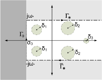
Figure 1: Regions of Zeros for $f(s)$

The following Lemma establishes the connection between the zeros of quasi-polynomial when $h=0$ and $h>0$.

Lemma 2.1

For any $\sigma_{0}\in\mathbb{R}$ which is smaller than minimum real part of roots of $a(s)+b(s)$, there exists $h>0$ such that the number of the zeros of the quasi-polynomial (2.1) are equal to the number of the zeros of $a(s)+b(s)$ in the region $\textrm{Re(s)}>\sigma_{0}$. All the infinitely many zeros of the quasi-polynomial (2.1) are in the complementary region, i.e., $\textrm{Re(s)}<\sigma_{0}$.

Proof 2.1.

Fix $\sigma_{0}$ as defined in the Lemma, since the degree of polynomial $a$ is larger than polynomial $b$, it is possible to choose $\omega_{*}$ large enough such that

$$\sup_{s\in\Gamma_{*}}\left|\frac{b(s)}{a(s)+b(s)}\right|<\epsilon_{*}$$

holds where $\Gamma_{*}=\{s\in\sigma+j\omega_{*}$ for $\sigma_{0}<\sigma<\infty\}$. Calculate

$$r_{0}\doteq\max_{s\in\Gamma_{0}}\left|\frac{b(s)}{a(s)+b(s)}\right|$$

where $\Gamma_{0}=\{s\in\sigma_{0}+j\omega$ for $-\omega_{*}<\omega<\omega_{*}\}$. The real number $r_{0}$ is well-defined since the curve $\Gamma_{0}$ passes from left of the zeros of the polynomial $a+b$. Choose $h$ small enough such that

$$\max_{s\in\Gamma_{0}}|e^{-hs}-1|<r_{0}^{-1}$$

is satisfied.

The functions $a(s)+b(s)$ and $b(s)(e^{-hs}-1)$ are analytic on and inside the contour $\Gamma=\Gamma_{0}\bigcup\Gamma_{*}\bigcup\bar{\Gamma}_{*}$. Note that on the contour $\Gamma$,

$$\max_{s\in\Gamma}\left|\frac{b(s)(e^{-hs}-1)}{a(s)+b(s)}\right|<1$$

holds. Using Rouché’s Theorem (see [5], Theorem 3.8) , the functions $a(s)+b(s)$ and $a(s)+b(s)e^{-hs}$ have the same number of zeros inside $\Gamma$. The light gray region of Figure 1 satisfies,

$$|a+be^{-hs}|>|b|(\epsilon_{*}^{-1}-1-e^{-h\sigma_{0}})>0$$

for sufficiently small $\epsilon_{*}$. Therefore, all other zeros lie in $\textrm{Re(s)}<\sigma_{0}$ which is dark gray region in Figure 1.

The Lemma 2.1 shows that for sufficiently small $h$, all the zeros of the quasi-polynomial (2.1) are close to the zeros of $a+b$ and all the other zeros can be pushed to the left by choosing smaller $h$. Therefore, one can choose the region large or small depending on requirements of stability analysis. This qualitative behavior makes boundary crossing detection possible.

The following Lemma can be used to calculate the distance of the zero of $f(s,h)$ from zero of $f(s,h+\Delta h)$.

Lemma 2.2.

Let $s_{i}^{h}$ be the zero of $f(s,h)$ (2.1), and $s_{i}^{h+\Delta h}$ be the zero of $f(s,h+\Delta h)$ where $s_{i}^{h}$ and $s_{i}^{h+\Delta h}$ are on the same trajectory. The distance between $s_{i}^{h}$ and $s_{i}^{h+\Delta h}$, i.e., $\delta_{i}=|\Delta s_{i}|=|s_{i}^{h+\Delta h}-s_{i}^{h}|$ is,

$$\delta_{i} \leq \frac{|s_{i}^{h}||\Delta h|}{\left|\frac{a^{\prime}(s_{i})}{a(s_{i})}-\frac{b^{\prime}(s_{i})}{b(s_{i})}+h\right|}+\mathcal{O}(|\Delta h|^{2})$$

where $\mathcal{O}()$ is the order function.

Proof 2.3.

Taylor expansion for $f(s,h)$ can be written as,

$$f(s_{i}^{h+\Delta h},h+\Delta h)=f(s_{i}^{h},h)+f_{s}(s_{i}^{h},h)\Delta s_{i}\\ +f_{h}(s_{i}^{h},h)\Delta h+\mathcal{O}(|\Delta h|^{2})$$ (2.2)

where $f_{s}$, $f_{h}$ are derivative of function $f(s,h)$ with respect to $s$ and $h$. Since $s_{i}^{h+\Delta h}$ and $s_{i}^{h}$ are zeros of $f(s,h)$,

$$0 = f_{s}(s_{i}^{h},h)\Delta s_{i}+f_{h}(s_{i}^{h},h)\Delta h+\mathcal{O}(|\Delta h|^{2}),$$

$$\Delta s_{i} = -\frac{f_{h}(s_{i}^{h},h)}{f_{s}(s_{i}^{h},h)}\Delta h+\mathcal{O}(|\Delta h|^{2}),$$ (2.3)

$$\delta_{i} \leq \left|\frac{f_{h}(s_{i}^{h},h)}{f_{s}(s_{i}^{h},h)}\right||\Delta h|+\mathcal{O}(|\Delta h|^{2}),$$

$$\delta_{i} \leq \left|\frac{-bs_{i}^{h}e^{-hs_{i}^{h}}}{a^{\prime}(s)+(b^{\prime}(s)-hb(s))e^{-hs_{i}^{h}}}\right||\Delta h|+\mathcal{O}(|\Delta h|^{2}),$$

$$\delta_{i} \leq \left|\frac{a(s_{i}^{h})s_{i}^{h}}{a^{\prime}(s_{i}^{h})-(\frac{b^{\prime}(s_{i}^{h})}{b(s_{i}^{h})}-h)a(s_{i}^{h})}\right||\Delta h|+\mathcal{O}(|\Delta h|^{2}).$$

The following section describes the method to find trajectories of quasi-polynomial zeros depending time-delay $h$. The convergence analysis of the method is given. All trajectories of the zeros except the asymptotic zeros are traced.

3 The Method and Analysis

3.1 Trajectory of Quasi-Polynomial Zero in the Region

Theorem 3.1.

Let $s_{i}^{h}$ be the zero of the quasi-polynomial (2.1). The trajectory of $s_{i}^{h}$ can be determined by the complex-valued ordinary differential equation,

$$\frac{ds}{dh}=-\left(\frac{f_{h}(s,h)+f(s,h)}{f_{s}(s,h)}\right),\quad s(h)=s_{i}^{h}$$ (3.4)

where $s$ is the trajectory of the zero and $s_{i}^{h}$ is the value when time-delay is equal to $h$. The trajectory is locally convergent to trajectory of zero.

Proof 3.2.

Define the local Lyapunov function $V(s,h)=\frac{1}{2}\overline{f(s,h)}f(s,h)$. Note that $V(s,h)$ is positive definite and assumes the value $0$ locally at the desired equilibrium $f(s,h)=0$.

$$\frac{dV(s,h)}{dh} = -Re(\overline{f(s,h)}(f_{s}(s,h)\frac{ds}{dh}+f_{h}(s,h)),$$

$$= -|f(s,h)|^{2}\leq 0.$$

Note that when the trajectory is close to local zero, it is convergent. When the trajectory coincides with the trajectory of the zero of the quasi-polynomial (2.1), using Taylor expansion one can show that

$$f(s_{i}^{h+\Delta h},h+\Delta h)\approx\mathcal{O}(|\Delta h|^{2}).$$ (3.5)

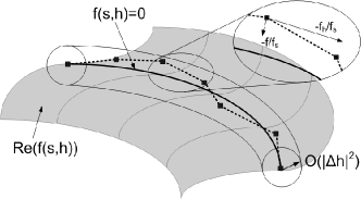
Figure 2: Trajectory of $f(s,h)$ zero on the $\textrm{Re}(f(s,h))$ surface

The exact solution of differential equation (3.4) follows the trajectory of the zero of the quasi-polynomial (2.1). Since the differential equation is solved by numerical methods in general, the solution is not exact and numerical errors are introduced due to step size of the numerical algorithm. However, the differential equation is numerically robust and the solution converges to trajectory of the zero of the quasi-polynomial locally and the algorithm decreases its error quadratically when step size is halved because of (3.5).

3.2 Quasi-Polynomial Zeros Crossing the Boundary

Given the region $\textrm{Re(s)}>\sigma_{0}$ for fixed $\sigma_{0}\in\mathbb{R}$, it is possible to trace the trajectory of roots in the region using (3.4) as time-delay $h$ changes. There may be additional zeros crossing the boundary $\textrm{Re(s)}=\sigma_{0}$ and entering into the region $\textrm{Re(s)}>\sigma_{0}$.

It is clear that when $h=0$, the zeros of quasi-polynomial in the region $\textrm{Re(s)}>\sigma_{0}$ are the roots of polynomial $a(s)+b(s)$ inside the region. The method traces all these zeros until they are outside the region. It is possible to find the zero-crossing frequencies $\omega_{i}$ on the boundary $s=\sigma_{0}+j\omega$ for $\omega\in\mathbb{R}$ using magnitude and phase equations as

$$0 = a(\sigma_{0}+j\omega)+b(\sigma_{0}+j\omega)e^{-h(\sigma_{0}+j\omega)},$$

$$h(\omega) = -\frac{\ln{\left|\frac{a(\sigma_{0}+j\omega)}{b(\sigma_{0}+j\omega)}\right|}}{\sigma_{0}},$$

$$0 = h(\omega)\omega+2k\pi+\angle{-\frac{a(\sigma_{0}+j\omega)}{b(\sigma_{0}+j\omega)}},\;k\in\mathbb{Z}.$$

The zero-crossing frequencies are $\omega_{i}\geq 0$ values such that the last equation is satisfied. Note that for each $\omega_{i}$, the corresponding time-delay $h(\omega_{i})$ should be positive. There are finitely many $\omega_{i}$ satisfying the equation for fixed time-delay value, $h$. When $\sigma_{0}=0$ is chosen, it is possible to find analytical method to calculate $\omega_{i}$ and corresponding $h(\omega_{i})$ as explained in [9].

The zeros of quasi-polynomial (2.1), $s=\sigma_{0}+j\omega_{i}$, cross the boundary at the time-delay values $h(\omega_{i})$ for $k=~{}1,\ldots,n_{h}$. However, we are interested in the characteristic roots crossing the boundary and entering into the region.

Corollary 3.3.

The zero of quasi-polynomial (2.1), $s=~{}\sigma_{0}+j\omega_{i}$, crosses the boundary and enters into the region $\textrm{Re(s)}>\sigma_{0}$ at the time-delay $h(\omega_{i})$ if

$$Re\left[\frac{1}{s}\left(\frac{b^{\prime}(s)}{b(s)}-\frac{a^{\prime}(s)}{a(s)}-h(\omega_{i})\right)\right]_{\begin{subarray}{c}s=\sigma_{0}+j\omega_{i}\end{subarray}}>0.$$ (3.6)

Proof 3.4.

The proof is based on [19] and some algebraic manipulations. One can show that

$$\frac{ds}{dh} = \frac{bse^{-hs}}{a^{\prime}(s)+(b^{\prime}(s)-hb(s))e^{-hs}},$$

$$= \frac{1}{\frac{1}{s}\left(\frac{a^{\prime}(s)}{b(s)e^{-hs}}+\left(\frac{b^{\prime}(s)}{b(s)}-h\right)\right)},$$

$$= \frac{1}{\frac{1}{s}\left(\frac{b^{\prime}(s)}{b(s)}-\frac{a^{\prime}(s)}{a(s)}-h\right)}.$$

The crossing zero enters the region if

$$Re\left(\left.\frac{ds}{dh}\right|_{\begin{subarray}{c}s=\sigma_{0}+j\omega_{i}\\ h=h(\omega_{i})\end{subarray}}\right)>0$$

which is equivalent to the condition (3.6).

The Corollary 3.3 is very important. It reduces the problem of the selection of the zeros entering into the region $\textrm{Re(s)}>\sigma_{0}$ into inequality condition (3.6) check for finite number of complex points, $s=j\omega_{i}$. Since we are interested in the zeros entering the region, define the zero-crossing points $s_{zc,k}=\sigma_{0}+j\omega_{k}$ satisfying Corollary 3.3. Note that the points $s_{zc,k}=\sigma_{0}+j\omega_{k}$ cross the boundary for time-delays $h(\omega_{i})$ for $k=1,\ldots,n_{zc}$.

3.3 The Method

Our objective is to find all the zeros of quasi-polynomial (2.1) in the region $\textrm{Re(s)}>\sigma_{0}$ when time-delay is equal to $h$.

1. Choose $\sigma_{0}\in\mathbb{R}$ according to design requirements,

2. Define the maximum error tolerance, $\epsilon_{tz}$, of the trajectory of the zero,

3. Calculate all the zero-crossing frequencies $\omega_{i}$ and the corresponding time-delay values $h(\omega_{i})$ for $i=1,\ldots,n_{h}$,

4. Select the zero-crossing frequencies satisfying (3.6) where the zeros enter into the region $\textrm{Re(s)}>\sigma_{0}$ (i.e., find $s_{sz,k}$ for $k=1,\ldots,n_{zc}$),

5. Define the delay set $\mathbf{h}=\{0\}\bigcup_{i=1}^{n_{zc}}\{h(\omega_{k})\}$ with elements in ascending order,

6. Define the set of zeros in the region $\textrm{Re(s)}>\sigma_{0}$ as $\mathbf{z}=\{z\in\mathbb{C},\;a(z)+b(z)=0,\textrm{Re(z)}>\sigma_{0}\}$ for $\mathbf{h}_{1}=0$,

7. Trace all the trajectories in the set $\mathbf{z}$ by (3.4) until next element of $\mathbf{h}$ (i.e., Runge-Kutta within the error tolerance $\epsilon_{tz}$). If any zero goes out of the region, drop the zero from the set $\mathbf{z}$. Add the new point $s=\sigma_{0}+j\omega_{i}$ for next element of $\mathbf{h}$ into the set $\mathbf{z}$. Repeat this step for all the elements of $\mathbf{h}$,

8. Trace the zeros in $\mathbf{z}$ until $h$. All the elements of $\mathbf{z}$ are the zeros of the quasi-polynomial (2.1) in the region $\textrm{Re(s)}>\sigma_{0}$.

Remarks:

1. The selection of $\sigma_{0}$ depends on objective of analysis. It can be selected close to imaginary axis to check the stability of the system. Since $\sigma_{0}$ can be chosen as desired, besides stability of the system, other stability criteria can be analyzed using our method such as damping criteria, $\mathcal{D}$-stability, fragility of the system, real stability distance, stability margins. It is possible to set $\sigma_{0}$ far from imaginary axis in the left half-plane such that the impulse response of the system is determined by zeros of the quasi-polynomial.

2. The boundary of the region is defined as straight line in this paper for convenience. It is possible to choose the boundary as a curve with imaginary part extending to infinity in magnitude and bounded real part (i.e., a boundary dividing the complex plane vertically). The only necessary restriction on boundary is to separate the complex plane into two regions and not extending to infinity in magnitude of real part where the quasi-polynomial has the infinitely many zeros. The boundary can be vertical any curve, any closed-curve (ellipse, circle).

3. Lemma 2.1 is essential to calculate the quasi-polynomial zeros crossing the boundary. It is guaranteed that when $h$ is small, all the zeros of quasi-polynomial are outside the region except the zeros of $a(s)+b(s)$ which are initially traced.

4. There are many methods in the literature to find the solution of the complex-valued differential equation (3.4) such as Runge-Kutta, Bulirsch-Stoer method, Adams methods [11]. In this paper, variable-step size $4^{\textrm{th}}$-order Runge-Kutta method is used. The algorithm is fast, easy to implement and robust due to local convergence of the trajectory of the quasi-polynomial zero shown in Theorem 3.1.

5. Instead of (3.4) which uses well-known Newton Algorithm in the literature for convergence to zero, there are other methods in the numerical analysis. Depending on the application and the quasi-polynomial (2.1), different algorithms may be used [11].

6. In our implementation, the delay step is adaptive in $4^{\textrm{th}}$-order Runge-Kutta method. If the next delay step is determined by

   $$\Delta h_{i+1}=\Delta h_{i}\sqrt{\frac{\epsilon_{tz}}{|f(s_{i}^{h_{i}})|}}$$

   where $s_{i}^{h_{i}}$ is the numerical solution of (3.4) at delay step $h_{i}$. Note that when the trajectory deviates from the tolerance for trajectory of the quasi-polynomial zero, the next step size is decreased with square root of the deviation due to (3.5). When the deviation of the trajectory of quasi-polynomial zero is smaller than tolerance, the step size is increased to reduce the computational effort.

7. There are numerical methods in the literature to calculate rightmost zeros of the quasi-polynomials approximately in the literature. Our method has two advantages:

   • It can be used to calculate zeros of the quasi-polynomial in any user-defined region.

   • In addition to zeros at time-delay $h$, we have all the location of the zeros of the quasi-polynomial in the region from $0$ to $h$ which is convenient when the delay effects on stability is analyzed.

4 Example

Consider the following time-delay system from [9]:

$$\dot{x}(t)=\left(\begin{array}[]{cc}0&1\\ -1&-1\end{array}\right)x(t)+\left(\begin{array}[]{cc}0&0\\ 0&-1\end{array}\right)x(t-\tau),\;\tau>0.$$

By analytical methods, it is shown that the system is stable $\tau\in[0,\pi)$ [9]. When $\tau=\pi$, the characteristic equation of the system has imaginary zeros, $s=\pm j$. We apply the method to find all the characteristic roots of the system for $\tau\in[0,\pi)$ in the region $\textrm{Re(s)}\geq-1$.

The characteristic quasi-polynomial can be found as

$$f(s,\tau)=(s^{2}+s+1)+se^{-\tau s}.$$

Following the algorithm in Section 3.3,

1. Define the region as $\textrm{Re(s)}\geq-1$ where $\sigma_{0}=-1$,

2. Error tolerance for trajectory is $\epsilon_{tz}=10^{-3}$,

3. Zero-crossing frequencies $\{\omega_{i}\}_{i=1}^{12}$ and the corresponding time-delays $\{h(\omega_{i})\}_{i=1}^{12}$ are given in Table 2,

4. The number of the zeros changes in the region when $\mathbf{h}=\{0\}\cup\{h(\omega_{i})\}_{i=0}^{12}$. The initial zeros in the region are $\mathbf{z}=\{-1.00,-1.00\}$ when $h=0$,

5. All the zeros of quasi-polynomial in the region $\textrm{Re(s)}>-1$ at $h=\pi$ are given in Table 2.

Table 1: Zero-crossing frequencies and the corresponding delays

$\omega_{i}$	$h(\omega_{i})$
$2.28$	$0.65$
$5.00$	$1.57$
$7.22$	$1.96$
$9.23$	$2.21$
$11.12$	$2.40$
$12.92$	$2.55$
$14.65$	$2.68$
$16.33$	$2.79$
$17.97$	$2.88$
$19.56$	$2.97$
$21.13$	$3.05$
$22.66$	$3.12$

Table 2: The zeros of quasi-polynomial in the region when $h=\pi$

$\pm j$

$-0.30,\pm 1.00j$

$-0.27\pm 2.60j$

$-0.47\pm 4.54j$

$-0.59\pm 6.52j$

$-0.68\pm 8.51j$

$-0.75\pm 10.51j$

$-0.80\pm 12.51j$

$-0.85\pm 14.50j$

$-0.89\pm 16.50j$

$-0.93\pm 18.50j$

$-0.96\pm 20.50j$

$-0.99\pm 22.50j$

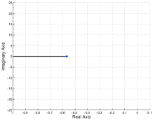
$\tau\in[0,0.5]$

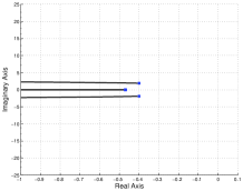
$\tau\in[0,1]$

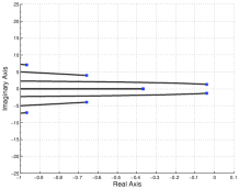
$\tau\in[0,2]$

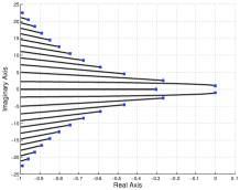
$\tau\in[0,\pi]$

Figure 3: Zeros of characteristic quasi-polynomial for different delay intervals

The trajectories of the zeros of the quasi-polynomial are shown in Figure 3. The system is stable for $\tau\in[0,\pi)$ as expected. When $\tau=\pi$, the system has imaginary roots $s=\pm j$. The system has characteristic zeros close to imaginary axis after $\tau>2.5$. Therefore, stability condition $\tau<\pi$ is conservative. The largest error in the trajectories is $7.6\;10^{-4}<\epsilon_{tz}$ as specified.

5 Concluding Remarks

We present a novel method to find the trajectories of all the zeros of the quasi-polynomial with single delay in predefined right half-plane. The method is an important tool for stability analysis of time-delay systems and effective for high-order systems.

Applications of the method to the zeros of the neutral type quasi-polynomials and multiple delay case are the future research directions and the results will be published elsewhere.

6 Acknowledgments

The author would like to thank M. L. Overton for his support.

References

- [1] S. Arunsawatwong, “Stability of retarded delay differential systems,” International Journal Of Control,, vol.65 (2), pp.347–364, 1996.
- [2] D. Breda, S. Maset and R. Vermiglio, “Computing the Characteristic Roots for Delay Differential Equations,” IMA Journal of Numerical Analysis, vol.24, pp.1–19, 2004.
- [3] D. Breda, S. Maset and R. Vermiglio, “Pseudospectral Differencing Methods for Characteristic Roots of Delay Differential Equations,” SIAM Journal on Scientific Computing, vol.27, pp.482–495, 2005.
- [4] D. Breda, “Solution Operator Approximations for Characteristic Roots of Delay Differential Equations,” Applied Numerical Mathematics, vol.56, pp.305–317, 2006.
- [5] J. B. Conway, Functions of One Complex Variable, 2nd ed., Graduate Texts in Mathematics, 11, Springer-Verlag, New York, 1978.
- [6] K. Engelborghs, T. Luzyanina and D. Roose, “Numerical Bifurcation Analysis of Delay Differential Equations,” Journal of Computational and Applied Mathematics, vol.125, pp.265–275, 2000.
- [7] K. Engelborghs and D. Roose, “On Stability of LMS Methods and Characteristics Roots of Delay Differential Equations,” SIAM Journal on Numerical Analysis, vol.40, pp.629–650, 2002.
- [8] P. Fu, S.-I. Niculescu, J. Chen, “Stability of linear neutral time-delay systems: exact conditions via matrix pencil solutions,” IEEE Transactions on Automatic Control, vol.51 (6), pp.1063-1069, 2006.
- [9] K. Gu, V. Kharitonov and J. Chen, Stability of Time-Delay Systems, Boston, MA: Birkh user, 2003.
- [10] Y. He, Q.-G. Wang, C. Lin, and M. Wu, “Augmented Lyapunov functional and delay-dependent stability criteria for neutral systems,”, International Journal of Robust and Nonlinear Control, vol.15 (18), pp.923–933, 2005.
- [11] J. D. Hoffman, Numerical Methods for Engineers and Scientists, New York, Marcel Dekker, 2001.
- [12] D. Ivanescu, S.-I. Niculescu, L. Dugard, J.-M. Dion, and E.I. Verriest, “On delay-dependent stability for linear neutral systems,” Automatica, vol.39 (2), pp.255–261, 2003.
- [13] G.-D. Hu and M. Liu, “Stability criteria of linear neutral systems with multiple delays,” IEEE Transactions on Automatic Control, vol.52 (4), pp.720-724, 2007.
- [14] H. Li, H-biao. Li and S. Zhong, “Stability of neutral type descriptor system with mixed delays,” Chaos, Solitons and Fractals Volume, vol.33 (5), pp.1796–1800, 2007.
- [15] S. I. Niculescu, Delay Effects on Stability: A Robust Control Approach. London: Springer-Verlag, 2001, vol.269, Lecture Notes in Control and Information Sciences.
- [16] N. Olgac and R. Sipahi, “A practical method for analyzing the stability of neutral type LTI-time delayed systems,” Automatica, vol.40 (5), pp.847–853, 2004.
- [17] J. P. Richard, “Time-Delay Systems: An Overview of Some Recent Advances and Open Problems,” Automatica, vol.39, pp.1667–1694, 2003.
- [18] G. J. Silva, A. Datta and S. P. Bhattacharyya, “New Results on the Synthesis of PID Controllers,” IEEE Transactions on Automatic Control, vol.47 (2), pp.241 -252, 2002.
- [19] R. Sipahi and N. Olgac, “Stability Robustness of Retarded LTI Systems with Single Delay and Exhaustive Determination of Their Spectra,” SIAM Journal on Control and Optimization, vol.45, pp.1680–1696, 2006.
- [20] K. Verheyden, T. Luzyanina and D. Roose, “Efficient Computation of Characteristic Roots of Delay Differential Equations using LMS Methods,” Journal of Computational and Applied Mathematics, vol.214, pp.209–226, 2008.