Virial coefficients of trapped and un-trapped three-component fermions
with three-body forces in arbitrary spatial dimensions

Abstract

Using a coarse temporal lattice approximation, we calculate the first few terms of the virial expansion of a three-species fermion system with a three-body contact interaction in $d$ spatial dimensions, both in homogeneous space as well as in a harmonic trapping potential of frequency $\omega$. Using the three-body problem to renormalize, we report analytic results for the change in the fourth- and fifth-order virial coefficients $\Delta b_{4}$ and $\Delta b_{5}$ as functions of $\Delta b_{3}$. Additionally, we argue that in the $\omega\to 0$ limit the relationship $b_{n}^{\text{T}}=n^{-d/2}b_{n}$ holds between the trapped (T) and homogeneous coefficients for arbitrary temperature and coupling strength (not merely in scale-invariant regimes). Finally, we point out an exact, universal (coupling- and frequency-independent) relationship between $\Delta b_{3}^{\text{T}}$ in 1D with three-body forces and $\Delta b_{2}^{\text{T}}$ in 2D with two-body forces.

I Introduction

Motivated by the recent interest in one-dimensional (1D) Fermi and Bose gases in the fine-tuned situation where only three-body interactions are present Nishida (2018); Pricoupenko (2018); Guijarro et al. (2018); Sekino and Nishida (2018); Valiente and Pastukhov (2019); McKenney and Drut (2019); Valiente (2019); Maki and Ordóñez (2019); Daza et al. (2019), we explore here the thermodynamics of fermions with a contact three-body interaction in the region of low fugacity (which corresponds to a dilute regime and therefore high temperatures in units of the energy scale set by the density). We focus on the fermionic case but explore the problem in arbitrary dimension $d$. To that end, we implement a semiclassical lattice approximation (SCLA) to calculate the virial coefficients $b_{n}$, and carry out their evaluation up to $n=5$ at leading order (LO) in that approximation.

The LO-SCLA was introduced in Ref. Shill and Drut (2018) as a way to estimate virial coefficients in two-component Fermi gases. The approximation seems crude in its definition but performs surprisingly well when the lowest non-trivial order in the virial expansion is used as a renormalized coupling constant ($b_{2}$ for two-body forces, for example, and $b_{3}$ in this work). Not surprisingly, the approximation was seen to work better at weak coupling, which makes sense as the radius of convergence of the virial expansion was found to be quickly reduced as a result of the interaction. In Ref. Hou et al. (2019), the NLO-SCLA was explored up to $b_{7}$, displaying the convergence properties up to the unitary point (in 3D) and in Ref. Morrell et al. (2019) the LO-SCLA was used for systems in a harmonic trap, showing that the approximation can capture the dependence on the trap frequency $\omega$. In both cases, the analytic dependence of virial coefficients on the dimension was obtained, as will be the case here. This is to be contrasted with conventional methods to calculate virial coefficients, which can be very precise but are limited to specific situations (coupling strength, dimension, etc.) and are typically unable to provide analytic insight as they are entirely numerical.

Our analytic formulas for the virial coefficients, although approximate, support and shed light on the relationship $b_{n}^{\text{T}}\to n^{-d/2}b_{n}$ in the $\omega\to 0$ limit, where the superindex T indicates the harmonically trapped situation. This connection is well-known to be valid in the noninteracting limit and in the so-called unitary limit of spin-$1/2$ fermions in 3D, both of which feature temperature-independent coefficients $b_{n}$. As we will argue, that relationship is actually valid for all temperatures and coupling constants, and holds for three-body interactions just as well as for two-body interactions. Finally, we point out an exact, coupling- and frequency-independent relationship between the $\Delta b_{3}^{\text{T}}$ in 1D with three-body forces and $\Delta b_{2}^{\text{T}}$ in 2D with two-body forces.

II Hamiltonian and virial expansion

We focus on a non-relativistic Fermi system with a three-body contact interaction, such that the Hamiltonian for three flavors $1,2,3$ is $\hat{H}=\hat{T}+\hat{V}$, where

$$\hat{T}\!=\!{\int{d^{d}x\,\hat{\psi}^{\dagger}_{s}({\bf x})\left(-\frac{\hbar^{2}\nabla^{2}}{2m}\right)\hat{\psi}_{s}({\bf x})}}$$ (1)

and

$$\hat{V}\!=\!-g_{d}\!\int{d^{d}x}\,\hat{n}_{1}({\bf x})\hat{n}_{2}({\bf x})\hat{n}_{3}({\bf x}),$$ (2)

where the field operators $\hat{\psi}_{s},\hat{\psi}^{\dagger}_{s}$ are fermionic fields for particles of type $1,2,3$ (summed over $s$ above), and $\hat{n}_{s}({\bf x})$ are the coordinate-space densities. In the remainder of this work, we will take $\hbar=k_{\text{B}}=m=1$. Besides the above, we will also consider the case in which an external trapping potential term is added to the Hamiltonian, of the form

$${\hat{V}}_{\text{ext}}\!=\!\frac{1}{2}m\omega^{2}\!\int{d^{d}x}\;{\bf x}^{2}\left[\hat{n}_{1}({\bf x})+\hat{n}_{2}({\bf x})+\hat{n}_{3}({\bf x})\right].$$ (3)

One way to characterize the thermodynamics is through the virial expansion Liu (2013), which is an expansion around the dilute limit $z\to 0$, where $z=e^{\beta\mu}$ is the fugacity, i.e. it is a low-fugacity expansion. The corresponding coefficients accompanying the powers of $z$ in the expansion of the grand-canonical potential $\Omega$ are the virial coeffiecients; specifically,

$$-\beta\Omega=\ln{\mathcal{Z}}=Q_{1}\sum_{n=1}^{\infty}b_{n}z^{n}$$ (4)

where

$$\mathcal{Z}=\mathrm{Tr}\left[e^{-\beta(\hat{H}-\mu\hat{N})}\right]=\sum_{N=0}^{\infty}z^{N}Q_{N}$$ (5)

is the grand-canonical partition function, $Q_{1}$ is the one-body partition function, $b_{1}=1$, and the higher-order coefficients require solving the corresponding few-body problems:

$$Q_{1}b_{2} = Q_{2}-\frac{Q_{1}^{2}}{2!},$$ (6)

$$Q_{1}b_{3} = Q_{3}-b_{2}Q_{1}^{2}-\frac{Q_{1}^{3}}{3!},$$ (7)

$$Q_{1}b_{4} = Q_{4}-\left(b_{3}+\frac{b_{2}^{2}}{2}\right)Q_{1}^{2}-b_{2}\frac{Q_{1}^{3}}{2!}-\frac{Q_{1}^{4}}{4!},$$ (8)

$$Q_{1}b_{5} = Q_{5}-(b_{4}+b_{2}b_{3})Q_{1}^{2}-\left(b_{2}^{2}+b_{3}\right)\frac{Q_{1}^{3}}{2}$$ (9)

$$-b_{2}\frac{Q_{1}^{4}}{3!}-\frac{Q_{1}^{5}}{5!},$$

and so forth.

Since $Q_{1}\propto V$, the above expressions display precisely how the volume dependence cancels out in each $b_{n}$. In particular, the highest power of $Q_{1}$ will always involve single-particle (i.e. noninteracting) physics and will therefore cancel in the change due to interactions $\Delta b_{n}$, such that

$$Q_{1}\Delta b_{2} = \Delta Q_{2}$$ (10)

$$Q_{1}\Delta b_{3} = \Delta Q_{3}-\Delta b_{2}Q_{1}^{2},$$ (11)

$$Q_{1}\Delta b_{4} = \Delta Q_{4}-\Delta\left(b_{3}+\frac{b_{2}^{2}}{2}\right)Q_{1}^{2}-\frac{\Delta b_{2}}{2}Q_{1}^{3},$$ (12)

$$Q_{1}\Delta b_{5} = \Delta Q_{5}-\Delta(b_{4}+b_{2}b_{3})Q_{1}^{2}$$ (13)

$$-\frac{1}{2}\Delta\left(b_{2}^{2}+b_{3}\right)Q_{1}^{3}-\frac{\Delta b_{2}}{3!}Q_{1}^{4},$$

and so on. Note that, when only three-body interactions are present, as is the case we consider here, there is no change in the two-body spectrum, i.e. $\Delta b_{2}=0$. Therefore, the above expressions simplify to

$$Q_{1}\Delta b_{3} = \Delta Q_{3},$$ (14)

$$Q_{1}\Delta b_{4} = \Delta Q_{4}-\Delta b_{3}Q_{1}^{2},$$ (15)

$$Q_{1}\Delta b_{5} = \Delta Q_{5}-\left(\Delta b_{4}+b_{2}\Delta b_{3}\right)Q_{1}^{2}-\frac{\Delta b_{3}}{2}Q_{1}^{3}.$$ (16)

In terms of the partition functions $Q_{MNL}$ of $M$ particles of type 1, $N$ of type 2, and $L$ of type $3$, we have

$$\Delta Q_{3} = \Delta Q_{111},$$ (17)

$$\Delta Q_{4} = 3\Delta Q_{211},$$ (18)

$$\Delta Q_{5} = 3\Delta Q_{311}+3\Delta Q_{221}.$$ (19)

From the above equations we see that there is only a small number of non-trivial contributions to each virial coefficient. The main task is calculating each of these terms and for that purpose we use a coarse lattice (or semiclassical) approximation, as explained next.

III The semiclassical approximation
at leading order

To carry out our calculations of virial coefficients we introduce a Trotter-Suzuki (TS) factorization of the Boltzmann weight. In the lowest possible order, the TS factorization amounts to keeping only the leading term in the following formula:

$$e^{-\beta(\hat{T}+\hat{V})}=e^{-\beta\hat{T}}e^{-\beta\hat{V}}\times e^{-\frac{\beta^{2}}{2}[\hat{T},\hat{V}]}\times\dots,$$ (20)

where higher orders involve exponentials of nested commutators of $\hat{T}$ with $\hat{V}$. Taking the leading order in this expansion is equivalent to setting $[\hat{T},\hat{V}]=0$, which is why we refer to it as a semiclassical approximation. As Refs. Shill and Drut (2018); Morrell et al. (2019); Hou et al. (2019) have shown, this seemingly crude approximation provides surprisingly good answers, especially at weak coupling, and is therefore useful toward examining the virial expansion in an analytic fashion. Below, we give two explicit examples of the application of our approximation to the calculation of virial coefficients.

III.1 A simple example: $\Delta b_{3}$

As the simplest example, we consider $Q_{111}$:

$$Q_{111} = \sum_{{\bf p}_{j}}\langle{\bf P}|e^{-\beta\hat{T}}e^{-\beta\hat{V}}|{\bf P}\rangle$$ (22)

$$\!\!\!\!\!\!\!\!\!\!\!\!=\sum_{{\bf p}_{j}}e^{-\beta(p_{1}^{2}+p_{2}^{2}+p_{3}^{2})/2m}\langle{\bf P}|e^{-\beta\hat{V}}|{\bf P}\rangle,$$

where we have used a collective momentum index ${\bf P}=({\bf p}_{1},{\bf p}_{2},{\bf p}_{3})$. Inserting a coordinate-space completeness relation to evaluate the potential energy factor, we obtain

$$e^{-\beta\hat{V}}|{\bf X}\rangle = \prod_{\bf z}(1+C\hat{n}_{1}({\bf z})\hat{n}_{2}({\bf z})\hat{n}_{3}({\bf z}))|{\bf X}\rangle$$

$$\!\!\!\!\!\!\!\!\!\!\!\!=|{\bf X}\rangle+C\sum_{\bf z}\delta({\bf x}_{1}-{\bf z})\delta({\bf x}_{2}-{\bf z})\delta({\bf x}_{3}-{\bf z})|{\bf X}\rangle$$

$$\!\!\!\!\!\!\!\!\!\!\!\!=\left[1+C\delta({\bf x}_{1}-{\bf x}_{3})\delta({\bf x}_{2}-{\bf x}_{3})\right]|{\bf X}\rangle,$$

where $C=(e^{\beta g_{d}}-1)\ell^{2d}$, $\ell$ is an ultraviolet regulator in the form of a spatial lattice spacing, and we used the fermionic relation $\hat{n}^{2}_{s}=\hat{n}_{s}$. We also introduced a collective index ${\bf X}=({\bf x}_{1},{\bf x}_{2},{\bf x}_{3})$. The $C$-independent term yields the noninteracting result, such that we may write

$$\Delta Q_{111} = C\sum_{{\bf p}_{j},{\bf x}_{k}}\!\!\!e^{-\beta(p_{1}^{2}+p_{2}^{2}+p_{3}^{2})/2m}$$ (24)

$$\times\delta({\bf x}_{1}-{\bf x}_{3})\delta({\bf x}_{2}-{\bf x}_{3})|\langle{\bf X}|{\bf P}\rangle|^{2},$$

which simplifies substantially when using a plane wave basis since $|\langle{\bf X}|{\bf P}\rangle|^{2}=1/V^{3}$, where $V$ is the $d$-dimensional volume of the system. We then find

$$\Delta Q_{111}=C\frac{Q_{100}^{3}}{V^{2}}$$ (25)

where

$$Q_{100}=\sum_{{\bf p}_{1}}e^{-\beta p_{1}^{2}/2m}.$$ (26)

Thus,

$$\Delta b_{3}=C\frac{{Q_{100}^{3}}}{V^{2}Q_{1}}=C\frac{Q_{1}^{2}}{27V^{2}}=\frac{C}{\lambda_{T}^{2d}}\frac{1}{3},$$ (27)

where $Q_{1}=3Q_{100}=3V/\lambda_{T}^{d}$, $\lambda_{T}=\sqrt{2\pi\beta}$ is the thermal wavelength, and $V$ is the system’s spatial volume. This relationship between the bare coupling constant $C$ and the physical quantity $\Delta b_{3}$ provides a way to renormalize the problem. In other words, $\Delta b_{3}$ will play the role of the renormalized dimensionless coupling constant.

The general form of the change $\Delta Q_{MNL}$ in the partition function for $M$ type-1 particles, $N$ type-2 particles and $L$ type-3 particles, with a contact interaction, is given by

$$\Delta Q_{MNL}=\sum_{{\bar{\bf P}},{\bar{\bf X}}}e^{-\beta{\bar{\bf P}}^{2}/2m}|\langle{\bar{\bf X}}|{\bar{\bf P}}\rangle|^{2}(Cf_{a}(\bar{\bf X})+C^{2}f_{b}(\bar{\bf X})+\dots),$$ (28)

where ${\bar{\bf P}},{\bar{\bf X}}$ represent all momenta and positions of the $M+N+L$ particles, and the functions $f_{a}$, $f_{b}$, $\dots$, which encode the matrix element of $e^{-\beta\hat{V}}$, depend on the specific $MNL$ case being considered. The wavefunction $\langle{\bar{\bf X}}|{\bar{\bf P}}\rangle$ is a product of three Slater determinants which, if using a plane-wave single-particle basis, leads to Gaussian integrals over the momenta $\bar{\bf P}$.

III.2 Another example: $\Delta b_{4}$ in a harmonic trap.

In this section we consider the case in which the system is held in a harmonic trapping potential of frequency $\omega$. As the expressions for the virial coefficients in terms of the canonical partition functions carry over to this case, we will simply add the superindex ‘T’ to denote quantities in the trapped system. To calculate $\Delta b_{4}^{\text{T}}$ we need $\Delta b_{3}^{\text{T}}$ and $Q_{1}^{\text{T}}$. The latter is of course trivial as there is no interaction in that case (see Ref. Morrell et al. (2019)):

$$Q_{1}^{\text{T}} = 3\sum_{\bf n}e^{-\beta E_{\bf n}}=3e^{-\beta\omega d/2}\bigg{(}\frac{1}{1-e^{-\beta\omega}}\bigg{)}^{d}$$ (29)

$$= 3\left(\frac{1}{2\sinh(\beta\omega/2)}\right)^{d},$$ (30)

where $E_{\bf n}$ is the single-particle energy level of the harmonic oscillator (separated in $d$-dimensional cartesian coordinates such that $\bf n$ represents a $d$-dimensional vector of harmonic oscillator quantum numbers).

To obtain $\Delta b_{3}^{\text{T}}$, we proceed as in the previous example to obtain the analogue of Eq. (24) for the trapped case:

$$\Delta Q^{\text{T}}_{111} = C\sum_{{\bf n}_{j},{\bf x}_{k}}\!\!\!e^{-\beta(E_{{\bf n}_{1}}+E_{{\bf n}_{2}}+E_{{\bf n}_{3}})}$$ (31)

$$\!\!\!\!\!\!\!\times\delta({\bf x}_{1}-{\bf x}_{3})\delta({\bf x}_{2}-{\bf x}_{3})|\langle{\bf x}_{1}{\bf x}_{2}{\bf x}_{3}|{\bf n}_{1}{\bf n}_{2}{\bf n}_{3}\rangle|^{2}.$$

The sums over ${\bf x}_{3},{\bf x}_{2}$ can be carried out right away, and moreover

$$|\langle{\bf x}_{1}{\bf x}_{2}{\bf x}_{3}|{\bf n}_{1}{\bf n}_{2}{\bf n}_{3}\rangle|^{2}=|\phi_{{\bf n}_{1}}({\bf x}_{1})|^{2}|\phi_{{\bf n}_{2}}({\bf x}_{2})|^{2}|\phi_{{\bf n}_{3}}({\bf x}_{3})|^{2},$$ (32)

where $\phi_{{\bf n}}({\bf x})$ is the single-particle harmonic oscillator wavefunction in $d$-dimensional cartesian coordinates. Using the above, we obtain

$$\Delta Q^{\text{T}}_{111} = C\sum_{{\bf x}}\rho^{3}({\bf x};\beta\omega),$$ (33)

where

$$\rho({\bf x};\beta\omega)=\sum_{{\bf n}}e^{-\beta E_{{\bf n}}}|\phi_{{\bf n}}({\bf x})|^{2}.$$ (34)

Note that $\sum_{\bf x}\rho({\bf x};\beta\omega)=Q_{1}^{\text{T}}/3$.

Using the Mehler kernel (see Ref. Morrell et al. (2019)) evaluated at equal spatial arguments, we find that

$$\rho({\bf x};\beta\omega)=\omega^{\frac{d}{2}}\frac{e^{-\omega\tanh(\beta\omega/2){\bf x}^{2}}}{\left(2\pi\sinh(\beta\omega)\right)^{\frac{d}{2}}},$$ (35)

where we note that $\tanh(\beta\omega/2)>0$ for all $\beta\omega>0$. Carrying out the resulting Gaussian integrals and simplifying,

$$\Delta b_{3}^{\text{T}}=\frac{\Delta Q^{T}_{111}}{Q_{1}^{\text{T}}}=\frac{C}{\lambda_{T}^{2d}}\frac{1}{3^{\frac{d}{2}+1}}\left(\frac{\beta\omega}{\sinh(\beta\omega)}\right)^{d},$$ (36)

where $\lambda_{T}=\sqrt{2\pi\beta}$.

Note that, as $\beta\omega\to 0$, we obtain

$$\Delta b_{3}^{\text{T}}=\frac{C}{\lambda_{T}^{2d}}\frac{1}{3^{\frac{d}{2}+1}}=\frac{1}{3^{\frac{d}{2}}}\Delta b_{3},$$ (37)

where in the last equality we have used Eq. (27).

For $\Delta b_{4}^{\text{T}}$, we need $\Delta Q^{\text{T}}_{211}$, which is easily seen to be given by

$$\Delta Q^{\text{T}}_{211} = C\sum_{{\bf x},{\bf x^{\prime}}}\rho^{2}({\bf x};\beta\omega)\left[\rho({\bf x};\beta\omega)\rho({\bf x}^{\prime};\beta\omega)-\rho^{2}({\bf x},{\bf x}^{\prime};\beta\omega)\right],$$ (38)

$$= \Delta Q^{\text{T}}_{111}Q_{1}^{\text{T}}/3-C\sum_{{\bf x},{\bf x^{\prime}}}\rho^{2}({\bf x};\beta\omega)\rho^{2}({\bf x},{\bf x}^{\prime};\beta\omega),$$

where

$$\rho({\bf x},{\bf x}^{\prime};\beta\omega)=\sum_{{\bf n}}e^{-\beta E_{{\bf n}}}\phi_{{\bf n}}({\bf x})\phi_{{\bf n}}({\bf x}^{\prime}),$$ (39)

which, using the Mehler kernel, becomes

$$\rho({\bf x},{\bf x}^{\prime};\beta\omega)=\frac{\omega^{\frac{d}{2}}e^{-\omega\coth(\beta\omega)({\bf x}^{2}+{\bf x}^{\prime 2})/2+\omega\operatorname{csch}(\beta\omega){\bf x}\cdot{\bf x}^{\prime}}}{\left(2\pi\sinh(\beta\omega)\right)^{\frac{d}{2}}}.$$ (40)

Thus, in the continuum limit,

$$\Delta b_{4}^{\text{T}} = 3\frac{\Delta Q^{T}_{211}}{Q_{1}^{\text{T}}}-\Delta b_{3}^{\text{T}}Q_{1}^{\text{T}}$$ (41)

$$= -\frac{3C}{Q_{1}^{\text{T}}}\sum_{{\bf x},{\bf x^{\prime}}}\rho^{2}({\bf x};\beta\omega)\rho^{2}({\bf x},{\bf x}^{\prime};\beta\omega)$$

$$= -\frac{C}{\lambda_{T}^{2d}}\frac{1}{2^{\frac{d}{2}}}\left[\frac{\beta\omega}{\sinh(\beta\omega)}\frac{1}{(1+3\cosh(\beta\omega))^{\frac{1}{2}}}\right]^{d}$$

$$= -\frac{3^{\frac{d}{2}+1}}{2^{\frac{d}{2}}}\frac{1}{(1+3\cosh(\beta\omega))^{\frac{d}{2}}}\Delta b_{3}^{\text{T}}.$$ (42)

Note that, in the $\beta\omega\to 0$ limit, our approximation yields

$$\Delta b_{4}^{\text{T}} = -\frac{3^{\frac{d}{2}}}{2^{d}}\frac{3}{2^{\frac{d}{2}}}\Delta b_{3}^{\text{T}}=-\frac{1}{2^{d}}\frac{3}{2^{\frac{d}{2}}}\Delta b_{3},$$ (43)

which we will use below.

IV Results in homogeneous space

IV.1 Virial coefficients

Using the steps outlined above, we have calculated $\Delta b_{4}$ and $\Delta b_{5}$ and obtained

$$\Delta b_{4} = -C\frac{Q_{1}Q_{1}(2\beta)}{9V^{2}}=-3\frac{Q_{1}(2\beta)}{Q_{1}}\Delta b_{3},$$ (44)

$$\Delta b_{5} = C\left(\frac{\left(Q_{1}(2\beta)\right)^{2}}{9V^{2}}+\frac{Q_{1}Q_{1}(3\beta)}{9V^{2}}\right)$$ (45)

$$= \left(\frac{3\left(Q_{1}(2\beta)\right)^{2}}{Q_{1}^{2}}+\frac{3Q_{1}(3\beta)}{Q_{1}}\right)\Delta b_{3},$$

for the fermionic three-species system with a three-body contact interaction in $d$ spatial dimensions. In the last equation, the first term on the right-hand side represents the contribution of $Q_{221}$, and the second term that of $Q_{311}$.

In the continuum limit, it is easy to perform the resulting Gaussian integrals that determine $Q_{1}$ and obtain

$$\Delta b_{4} = -\frac{3}{2^{\frac{d}{2}}}\Delta b_{3},$$ (46)

$$\Delta b_{5} = 3\left(\frac{1}{2^{d}}+\frac{1}{3^{\frac{d}{2}}}\right)\Delta b_{3}.$$ (47)

Using these results, one may calculate the pressure, density, compressibility and even Tan’s contact (with knowledge of $\Delta b_{3}$ as a function of the interaction strength, e.g. $\beta\epsilon_{B}$ in 1D or 2D, where $\epsilon_{B}$ is the trimer binding energy). To provide a description of the thermodynamics that is as universal as possible across spatial dimensions, we will use $\Delta b_{3}$ as the measure of the interaction strength and display our results in terms of that parameter. Furthermore, one may also define a (dimensionless) contact density as

$$\mathcal{C}=\frac{\lambda_{T}^{d}}{V}\frac{\mathcal{\partial}\ln\mathcal{Z}}{\partial\Delta b_{3}},$$ (48)

which differs from the conventional definition by a chain-rule factor ${\partial\Delta b_{3}}/{\partial\lambda}$ (which in turn can be determined by solving the three-body scattering problem), where $\lambda$ is the $d$-dimensional coupling constant. To make the expression dimensionless, we have used the thermal wavelength $\lambda_{T}=\sqrt{2\pi\beta}$.

IV.2 Thermodynamics and contact across dimensions

The interaction change in the pressure $\Delta P$ can be written in dimensionless form in arbitrary dimension as

$$\beta V\Delta P=Q_{1}\sum_{k=1}^{\infty}\Delta b_{k}\,z^{k}.$$ (49)

Similarly, the interaction change in the density can be written as

$$\lambda_{T}^{d}\Delta n=3\sum_{k=1}^{\infty}k\,\Delta b_{k}\,z^{k},$$ (50)

and, using our definition of the contact in Eq. (48),

$$\Delta\mathcal{C}=3\sum_{k=1}^{\infty}\frac{\partial\Delta b_{k}}{\partial\Delta b_{3}}\,z^{k}.$$ (51)

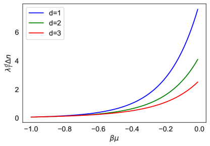
Figure 1: Density, in units of $\lambda^{d}_{T}=(2\pi\beta)^{d/2}$ as a function of $\ln z=\beta\mu$, at $\Delta b_{3}=0.25$.

Implementing our LO-SCLA results, we obtain

$$\beta\lambda_{T}^{d}\Delta P \simeq 3\Delta b_{3}\,z^{3}\!\!\left[1-\frac{3}{2^{\frac{d}{2}}}z+3\left(\!\frac{1}{2^{d}}+\frac{1}{3^{\frac{d}{2}}}\!\right)z^{2}\right],$$ (52)

$$\lambda_{T}^{d}\Delta n \simeq 9\,\Delta b_{3}\,z^{3}\!\!\left[1-\frac{4}{2^{\frac{d}{2}}}z+5\left(\!\frac{1}{2^{d}}+\frac{1}{3^{\frac{d}{2}}}\!\right)z^{2}\right],$$ (53)

$$\Delta\mathcal{C} \simeq 3z^{3}\left[1-\frac{3}{2^{\frac{d}{2}}}z+3\left(\!\frac{1}{2^{d}}+\frac{1}{3^{\frac{d}{2}}}\!\right)z^{2}\right].$$ (54)

As an example, in Fig. 1 we display the density as a function of the logarithm of the fugacity $\ln z=\beta\mu$ for $\Delta b_{3}=0.25$ and for $d=1,2,3$.

The behavior of $\Delta n$ as a function of $\beta\mu$ in Fig. 1 is as expected for a system with attractive interactions, namely the interaction-induced change in the density is positive and enhanced by increasing $\beta\mu$ (or, equivalently, washed out at low densities, i.e. for large and negative $\beta\mu$). Also as expected (and as observed in Refs. Shill and Drut (2018) and Hou et al. (2019) for two-body interactions), interaction effects are more pronounced in lower dimensions at fixed $\Delta b_{3}$.

V Results in a harmonic trap

V.1 Fourth- and fifth-order virial coefficients

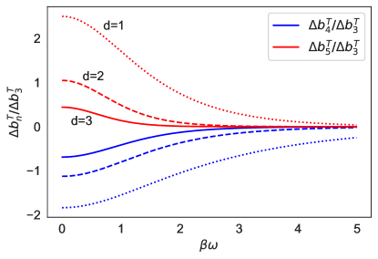
Figure 2: $\Delta b_{4}^{T}$ (blue lines) and $\Delta b_{5}^{T}$ (red lines), in units of $\Delta b_{3}^{T}$, as a function of $\beta\omega$ in the LO-SCLA. Results are shown in $d=1$ (dotted), $d=2$ (dashed), and $d=3$ (solid).

We have generalized our example of $\Delta b_{4}^{\text{T}}$, discussed in a previous section, to $\Delta b_{5}^{\text{T}}$. For future reference, we show both results:

$$\Delta b_{4}^{\text{T}} = -\frac{3^{\frac{d}{2}+1}}{2^{\frac{d}{2}}}\frac{1}{(1+3\cosh(\beta\omega))^{\frac{d}{2}}}\Delta b_{3}^{\text{T}},$$ (55)

$$\Delta b_{5}^{\text{T}} = 3^{\frac{d}{2}+1}\left(\left[\frac{1}{12\cosh^{2}(\beta\omega)+4\cosh(\beta\omega)-1}\right]^{\frac{d}{2}}\right.$$ (56)

$$+ \left.\left[\frac{1}{12\cosh^{2}(\beta\omega)+8\cosh(\beta\omega)}\right]^{\frac{d}{2}}\right)\Delta b_{3}^{\text{T}}.$$

In Fig. 2 we show these results in $d=1,2,3$ as a function of $\beta\omega$. In contrast to the behavior of $\Delta b_{4}^{T}$ for the case of two-body interactions, explored in Refs. Yan and Blume (2016); Morrell et al. (2019), here both $\Delta b_{4}^{\text{T}}$ and $\Delta b_{5}^{\text{T}}$ display monotonic behavior. Furthermore, at this order in the SCLA, both $\Delta b_{4}^{\text{T}}$ and $\Delta b_{5}^{\text{T}}$ are proportional to $\Delta b_{3}^{\text{T}}$, such that the results of Fig. 2 are universal predictions in the sense of being coupling-independent.

V.2 A universal relation in the $\beta\omega\to 0$ limit

Note that, in the $\beta\omega\to 0$ limit, where the homogeneous system is recovered,

$$\Delta b_{5}^{\text{T}}\to 3^{\frac{d}{2}+1}\frac{1}{5^{\frac{d}{2}}}\left(\frac{1}{2^{d}}+\frac{1}{3^{\frac{d}{2}}}\right)\Delta b_{3}^{\text{T}}=\frac{3}{5^{\frac{d}{2}}}\left(\frac{1}{2^{d}}+\frac{1}{3^{\frac{d}{2}}}\right)\Delta b_{3}$$ (57)

Using Eqs. (43), (46), and (57), we find that trapped and un-trapped virial coefficients are related, in the $\beta\omega\to 0$ limit, as follows:

$$\Delta b_{3}^{\text{T}} = 3^{-\frac{d}{2}}\Delta b_{3},$$ (58)

$$\Delta b_{4}^{\text{T}} = 4^{-\frac{d}{2}}\Delta b_{4},$$ (59)

$$\Delta b_{5}^{\text{T}} = 5^{-\frac{d}{2}}\Delta b_{5}.$$ (60)

Although we have only explored $\Delta b_{n}^{\text{T}}$ for $n=3,4,5$ here (the cases $n=1,2$ are trivially satisfied as well), the fact that the above relationship holds points us to conjecture that the relation

$$\left.b_{n}^{\text{T}}\right|_{\beta\omega\to 0}=n^{-\frac{d}{2}}b_{n},$$ (61)

is universally valid for all $n$, couplings, and temperatures (it is well known to be satisfied by noninteracting gases). Other authors, see e.g. Liu et al. (2009, 2010); Liu (2013) have noted (and proven using the local density approximation) that this relationship is satisfied in the unitary limit (where the $b_{n}$ are temperature-independent), and the same connection was found for $n=3,4$ in systems with two-body forces in Ref. Morrell et al. (2019) for arbitrary couplings (within the LO-SCLA). In principle, there is no special reason why $b_{n}^{\text{T}}$ should not approach $b_{n}^{\text{}}$ when the trapping potential is removed. That there is a $d$- and $n$-dependent factor connecting those two quantities in the noninteracting case is merely a geometrical artifact of the choice of basis in which the calculations are performed (namely the harmonic oscillator basis in the trapped case and plane waves in the homogeneous case), which has no impact on physical quantities. Based entirely on dimensional analysis, however, the natural guess is that $b_{n}^{\text{T}}$ may approach $b_{n}^{\text{}}$ times a dimensionless function of temperature and other dynamical scales. [That would actually change the partition function in a non-trivial way, in particular concerning Tan’s contact, but let us put that aside for the moment.] Such a dimensionless function could only result from the interplay between the trapping potential ${\hat{V}}_{\text{ext}}$ and the interaction $\hat{V}$, possibly leading to subtleties in the $\omega\to 0$ limit (similar to those arising from degenerate perturbation theory). However, the fact that $[{\hat{V}}_{\text{ext}},\hat{V}]=0$ suggests that there should be no such subtlety and therefore no residual dependence on interaction-related scales in the relationship between $b_{n}^{\text{T}}$ and $b_{n}$ as $\beta\omega\to 0$. In that limit, the dimensionless quantities $b_{n}^{\text{T}}$ and $b_{n}$ should be related by a coupling- and temperature-independent function; their connection should be entirely geometrical and fully determined by the noninteracting case, for which $b_{n}^{\text{T}}=n^{-\frac{d}{2}}b_{n}$ when $\beta\omega\to 0$. We therefore conclude that the conjecture is true for all $n$, coupling strengths, and temperatures.

V.3 An exact relation across systems and dimensions

Finally, we point out a coupling-independent relationship between the 1D case with a three-body interaction (i.e. the 1D case of the system studied in this work) and the 2D case with only two-body interactions (denoted below by the superindex “2b2D”). As pointed out in Ref. Drut et al. (2018), there exists an exact relationship between the three-body problem of the former situation and the two-body problem of the latter. That relationship yields a simple proportionality rule between the corresponding virial coefficients, given by

$$\Delta b_{3}=\frac{Q_{111}^{\text{cm}}}{Q_{11}^{\text{cm, 2b2D}}}\frac{Q_{1}^{\text{2b2D}}}{Q_{1}}\Delta b_{2}^{\text{2b2D}},$$ (62)

where the superscript “cm” indicates the partition function associated with the center-of-mass motion, which is not affected by the interactions and completely factorizes (both in the spatially homogeneous as well as in the harmonically trapped case). In the spatially homogeneous case, the proportionality factor between $\Delta b_{3}$ and $\Delta b_{2}^{\text{2b2D}}$ is $1/\sqrt{3}$, as shown in Ref. Drut et al. (2018). On the other hand, in the harmonically trapped case, the relationship becomes

$$\Delta b_{3}^{\text{T}}=\frac{2}{3}\Delta b_{2}^{\text{T,2b2D}}.$$ (63)

We stress that while this relationship is restricted to the 1D $\Delta b_{3}^{\text{T}}$ and $\Delta b_{2}^{\text{T,2b2D}}$, it is valid for all couplings and all values of $\beta\omega$ and is in that sense universal.

For completeness and future reference, we provide here details on the origin of this correspondence for the trapped case. The Schrödinger equation for this system takes the form

$$\left[-\frac{\nabla^{2}_{\bf r}}{2m}+\frac{g}{m}\delta(x-y)\delta(y-z)+\frac{1}{2}m\omega^{2}{\bf r}^{2}\right]\psi({\bf r})=E\psi({\bf r})$$ (64)

where $x$, $y$, and $z$ again indicate the different-flavor particles, ${\bf r}=(x,y,z)$, and

$$\nabla^{2}_{\bf r}=\frac{\partial^{2}}{\partial x^{2}}\!+\!\frac{\partial^{2}}{\partial y^{2}}\!+\!\frac{\partial^{2}}{\partial z^{2}}.$$ (65)

Factoring out the center-of-mass (c.m.) motion by defining $Q=\frac{1}{\sqrt{3}}(x+y+z)$, $q_{1}=\frac{1}{\sqrt{2}}(y-x)$, $q_{2}=\frac{1}{\sqrt{6}}(x+y-2z)$, and $\psi(x,y,z)=\Phi(Q)\phi({\bf q})$, with ${\bf q}=(q_{1},q_{2})$, we obtain

$$\left[-\frac{1}{2m}\frac{\partial^{2}}{\partial Q^{2}}+\frac{1}{2}m\omega^{2}Q^{2}\right]\Phi(Q)=E_{\mathrm{c.m.}}\Phi(Q),$$ (66)

for the c.m. motion, and

$$\left[-\frac{\nabla^{2}_{\bf q}}{2m}+\frac{\tilde{g}}{m}\delta({\bf q})+\frac{1}{2}m\omega^{2}{\bf q}^{2}\right]\phi({\bf q})=E_{r}\phi({\bf q}),$$ (67)

where $\displaystyle\tilde{g}={g}/{\sqrt{3}}$ is the effective coupling and $E_{r}$ is the energy of relative motion, which is identical to that of a single particle in a 2D harmonic oscillator potential with a $\delta$-potential at the origin. This establishes the exact relationship between our three-body 1D problem and its two-body counterpart in 2D with two-body interactions.

As in the spatially homogeneous case, the eigenvalues $\epsilon_{\omega}=E_{r}/\omega$ of the harmonically trapped system are determined implicitly, in this case as solutions to

$$\frac{1}{\tilde{g}}=\frac{1}{\pi}\sum_{n=0}^{\Lambda_{\omega}}\frac{1}{\epsilon_{\omega}-(2n+1)}\rightarrow\frac{1}{2\pi}\left[\psi_{0}\left(\frac{1-\epsilon_{\omega}}{2}\right)-\ln{\Lambda_{\omega}}\right],$$ (68)

where $\psi_{0}(z)$ is the digamma function, where $\Lambda_{\omega}$ is a UV cutoff. Unlike in the untrapped problem, with its unique bound state, the trapped problem admits an infinite set of discrete excited states (all with positive energy). The problem is renormalized by relating the bare coupling to the $\epsilon_{\omega}$ occurring in the lowest energy branch.

VI Summary and Conclusions

In this work we have calculated the high-temperature thermodynamics of three-flavored Fermi gases with a contact three-body interaction in $d$ spatial dimensions, as determined by the virial expansion. We carried out calculations in homogeneous space as well as in a harmonic trapping potential of frequency $\omega$. To that end, we implemented a coarse temporal lattice approximation at leading order (the LO-SCLA) and calculated the change in the virial coefficients $\Delta b_{n}$ due to interaction effects. In that context, we established a relation between the first two non-trivial virial coefficients, namely $\Delta b_{4}$ and $\Delta b_{5}$, as functions of $\Delta b_{3}$. In addition, we argued that in the $\beta\omega\to 0$ limit, the relationship $\Delta b_{n}^{\text{T}}=n^{-d/2}\Delta b_{n}$ holds between the trapped and homogeneous coefficients for arbitrary $n$, coupling strengths, and temperatures; furthermore, it is valid for systems with two- and three-body interactions. We showed that our calculations reproduce that relationship for $n=3,4,5$. Finally, we showed a relationship between the harmonically trapped case in 1D with three-body interactions and its analogue in 2D with two-body interactions, namely $\Delta b_{3}^{\text{T}}=\frac{2}{3}\Delta b_{2}^{\text{T,2b2D}}$.

References

• Nishida (2018) Yusuke Nishida, “Universal bound states of one-dimensional bosons with two- and three-body attractions,” Phys. Rev. A 97, 061603 (2018).
• Pricoupenko (2018) Ludovic Pricoupenko, “Pure confinement-induced trimer in one-dimensional atomic waveguides,” Phys. Rev. A 97, 061604 (2018).
• Guijarro et al. (2018) G. Guijarro, A. Pricoupenko, G. E. Astrakharchik, J. Boronat,  and D. S. Petrov, “One-dimensional three-boson problem with two- and three-body interactions,” Phys. Rev. A 97, 061605 (2018).
• Sekino and Nishida (2018) Yuta Sekino and Yusuke Nishida, “Quantum droplet of one-dimensional bosons with a three-body attraction,” Phys. Rev. A 97, 011602 (2018).
• Valiente and Pastukhov (2019) M. Valiente and V. Pastukhov, “Anomalous frequency shifts in a one-dimensional trapped bose gas,” Phys. Rev. A 99, 053607 (2019).
• McKenney and Drut (2019) J. R. McKenney and J. E. Drut, “Fermi-Fermi crossover in the ground state of one-dimensional few-body systems with anomalous three-body interactions,” Phys. Rev. A99, 013615 (2019)arXiv:1811.05418 [cond-mat.quant-gas] .
• Valiente (2019) M. Valiente, “Three-body repulsive forces among identical bosons in one dimension,” Phys. Rev. A 100, 013614 (2019).
• Maki and Ordóñez (2019) Jeff Maki and Carlos R. Ordóñez, “Virial expansion for a three-component fermi gas in one dimension: The quantum anomaly correspondence,” Phys. Rev. A 100, 063604 (2019).
• Daza et al. (2019) W. S. Daza, J. E. Drut, C. L. Lin,  and Carlos R. Ordóñez, “A Quantum Field-Theoretical Perspective on Scale Anomalies in 1D systems with Three-Body Interactions,” Mod. Phys. Lett. A34, 1950291 (2019)arXiv:1808.07011 [hep-th] .
• Shill and Drut (2018) C. R. Shill and J. E. Drut, “Virial coefficients of one-dimensional and two-dimensional fermi gases by stochastic methods and a semiclassical lattice approximation,” Phys. Rev. A 98, 053615 (2018).
• Hou et al. (2019) Y. Hou, A. J. Czejdo, J. DeChant, C. R. Shill,  and J. E. Drut, “Leading- and next-to-leading-order semiclassical approximation to the first seven virial coefficients of spin-1/2 fermions across spatial dimensions,” Phys. Rev. A 100, 063627 (2019).
• Morrell et al. (2019) K. J. Morrell, C. E. Berger,  and J. E. Drut, “Third- and fourth-order virial coefficients of harmonically trapped fermions in a semiclassical approximation,” Phys. Rev. A 100, 063626 (2019).
• Liu (2013) Xia-Ji Liu, “Virial expansion for a strongly correlated fermi system and its application to ultracold atomic fermi gases,” Physics Reports 524, 37 – 83 (2013), virial expansion for a strongly correlated Fermi system and its application to ultracold atomic Fermi gases.
• Yan and Blume (2016) Yangqian Yan and D. Blume, “Path-integral monte carlo determination of the fourth-order virial coefficient for a unitary two-component fermi gas with zero-range interactions,” Phys. Rev. Lett. 116, 230401 (2016).
• Liu et al. (2009) Xia-Ji Liu, Hui Hu,  and Peter D. Drummond, “Virial expansion for a strongly correlated fermi gas,” Phys. Rev. Lett. 102, 160401 (2009).
• Liu et al. (2010) Xia-Ji Liu, Hui Hu,  and Peter D. Drummond, “Three attractively interacting fermions in a harmonic trap: Exact solution, ferromagnetism, and high-temperature thermodynamics,” Phys. Rev. A 82, 023619 (2010).
• Drut et al. (2018) J. E. Drut, J. R. McKenney, W. S. Daza, C. L. Lin,  and C. R. Ordóñez, “Quantum anomaly and thermodynamics of one-dimensional fermions with three-body interactions,” Phys. Rev. Lett. 120, 243002 (2018).