The Discrete-Time Facilitated Totally Asymmetric Simple Exclusion Process

Abstract

We describe the translation invariant stationary states of the one dimensional discrete-time facilitated totally asymmetric simple exclusion process (F-TASEP). In this system a particle at site $j$ in $\mathbb{Z}$ jumps, at integer times, to site $j+1$, provided site $j-1$ is occupied and site $j+1$ is empty. This defines a deterministic noninvertible dynamical evolution from any specified initial configuration on $\{0,1\}^{\mathbb{Z}}$. When started with a Bernoulli product measure at density $\rho$ the system approaches a stationary state, with phase transitions at $\rho=1/2$ and $\rho=2/3$. We discuss various properties of these states in the different density regimes $0<\rho<1/2$, $1/2<\rho<2/3$, and $2/3<\rho<1$; for example, we show that the pair correlation $g(j)=\langle\eta(i)\eta(i+j)\rangle$ satisfies, for all $n\in\mathbb{Z}$, $\sum_{j=kn+1}^{k(n+1)}g(j)=k\rho^{2}$, with $k=2$ when $0\leq\rho\leq 1/2$ and $k=3$ when $2/3\leq\rho\leq 1$, and conjecture (on the basis of simulations) that the same identity holds with $k=6$ when $1/2\leq\rho\leq 2/3$. The $\rho<1/2$ stationary state referred to above is also the stationary state for the deterministic discrete-time TASEP at density $\rho$ (with Bernoulli initial state) or, after exchange of particles and holes, at density $1-\rho$.

Keywords: Totally asymmetric exclusion processes, one dimensional conserved lattice gas, facilitated jumps, non-invertible deterministic evolution, phase transitions, traffic models

AMS subject classifications: 60K35, 82C22, 82C23, 82C26

1 Introduction

The facilitated totally asymmetric simple exclusion process (F-TASEP) is a model of particles moving on the lattice $\mathbb{Z}$, in which a particle at site $j$ jumps, at integer times, to site $j+1$, provided site $j-1$ is occupied and site $j+1$ is empty; many of the results on this model appeared in [9], without complete proofs. The related model in which the discrete time steps are replaced by a continuous time evolution has been studied both numerically and analytically [2, 6, 8], as has the continuous-time model with symmetric evolution [5, 16]. There are extensive numerical simulations of similar models (usually called Conserved Lattice Gases) in two or more dimensions [11, 14, 18], but there are few analytic results (but see [19]). The model is of interest in part because it exhibits nonequilibrium phase transitions.

A configuration of the model is an arrangement of particles on $\mathbb{Z}$, with each site either empty or occupied by a single particle; that is, the configuration space is $X=\{0,1\}^{\mathbb{Z}}$, with 1 denoting the presence of a particle and 0 that of a hole. We write $\eta=(\eta(i))_{i\in\mathbb{Z}}$ for a typical configuration, and for $j,k\in\mathbb{Z}$ with $j\leq k$ we let $\eta\hbox{$(j\!:\!k)$}=(\eta(i))_{j\leq i\leq k}$ denote the portion of the configuration lying between sites $j$ and $k$ (inclusive). We will occasionally use string notation, and correspondingly concatenation, for configurations or partial configurations, writing for example $\eta\hbox{$(0\!:\!6)$}=\eta(0)\cdots\eta(6)=0\,1\,1\,0\,1\,0\,1=01^{2}(01)^{2}$. For $0\leq\rho\leq 1$ we let $X_{\rho}\subset X$ denote the set of configurations with a well-defined density $\rho$, that is, configurations $\eta$ for which

$$\lim_{N\to\infty}\frac{1}{N}\sum_{i=1}^{N}\eta(i)=\lim_{N\to\infty}\frac{1}{N}\sum_{i=-N}^{-1}\eta(i)=\rho.$$ (1.1)

Here we study the F-TASEP discrete-time dynamics as described above. For $\rho\notin\{1/2,2/3\}$ we will determine the ultimate fate of any initial configuration $\eta\in X_{\rho}$. We will also describe the translation invariant (TI) states (i.e., TI probability measures on $X$) of the system which are stationary under the dynamics (the TIS states); without loss of generality we restrict consideration to states for which almost all configurations have the same well-defined density $\rho$, called states of density $\rho$, and will frequently assume further that these states are ergodic under translations. We would also like to determine the final TIS state when the dynamics is started in a Bernoulli measure: an initial state $\mu^{(\rho)}$ for which each site is independently occupied with probability $\rho$. In this, however, we will not be completely successful.

We will make use of a closely related model, the totally asymmetric stack model (TASM), another particle system on $\mathbb{Z}$ evolving in discrete time. In the TASM there are no restrictions on the number of particles at any site, so that the configuration space is $Y=\mathbb{Z}_{+}^{\mathbb{Z}}$, where $\mathbb{Z}_{+}=\{0,1,2,\ldots\}$. We denote stack configurations by boldface letters, so that a typical configuration is ${\bf n}=({\bf n}(i))_{i\in\mathbb{Z}}$. The dynamics is as follows: at each integer time, every stack with at least two particles (${\bf n}(i)\geq 2$) sends one particle to the neighboring site to its right. This model is thus essentially a discrete-time zero range process.

There is a natural correspondence between the TASM and the F-TASEP, with a stack configuration ${\bf n}$ corresponding to a particle configuration in which successive strings of ${\bf n}(i)$ particles are separated by single holes; as just stated the correspondence is somewhat loose but yields a bijective map $\psi:X^{(0)}\to Y$, where $X^{(0)}\subset X$ is the set of F-TASEP configurations $\eta$ satisfying $\eta(0)=0$. Moreover, if $\mu$ is a TI probability measure on $X$ and we define $\hat{\mu}=\mu(X^{(0)})^{-1}\mu\circ\psi^{-1}$ then $\mu\mapsto\hat{\mu}$ is a bijective correspondence between TI, or TIS, probability measures on $Y$ and on $X$; this correspondence is discussed in detail in Section 2.1. Using it, we show in Section 2.2 that there are three phases for the F-TASEP, that is, three distinct regimes in which the model exhibits qualitatively different behavior: the regions of low, intermediate, and high density in which respectively $0<\rho<1/2$, $1/2<\rho<2/3$, and $2/3<\rho<1$.

In subsequent sections we show, for each density region, how to determine the “final configuration” resulting from the evolution of some arbitrary initial configuration; we then suppose that the initial configuration has a Bernoulli distribution and study the distribution of the final configuration—that is, the TIS measure which is the $t\to\infty$ limit of an initial Bernoulli measure (this problem was studied for the continuous time model in [6]). It is for the low density phase, treated in Section 3, that we can say the most. We show that every initial configuration $\eta_{0}$ of density $\rho<1/2$ has a limit $\eta_{\infty}$—that is, it eventually freezes—and compute, for a Bernoulli initial measure, the distribution of these final configurations, which arises from a certain renewal process. Moreover, we show that if site $i$ is a point of this renewal process then the expected density at any site an odd distance ahead of $i$ is $\rho$, and that the two-point function in the final state, $g(i)=\langle\eta_{\infty}(j)\eta_{\infty}(i+j)\rangle$, satisfies $g(2n-1)+g(2n)=2\rho^{2}$ for any $n\geq 1$; the latter property implies that the asymptotic value of $V_{L}/L$, where $V_{L}$ is the variance of the number of particles in an interval of length $L$, has the same value $\rho(1-\rho)$ as for the initial Bernoulli measure. We also compute the distribution of the distance moved by a typical particle through the evolution and find that the expected value of this distance is finite. Finally, we show (see Remark 3.10) that the $\rho<1/2$ stationary state is also the stationary state for the deterministic discrete-time totally asymmetric simple exclusion process (TASEP) at density $\rho$ (in each case with Bernoulli initial state) or, after exchange of particles and holes, at density $1-\rho$.

A key technique for the study of the intermediate and high density regions is to consider the dynamics in a moving frame; it is in this frame that a limiting configuration exists for each initial configuration. Rather surprisingly, perhaps, the behavior of the model in the high density region is largely parallel to that in the low density region; we thus content ourselves with a rather brief treatment in Section 4. For the intermediate region, discussed in Section 5, the dynamics is considerably more complicated. Here we are able to carry out the second step of the program, that is, to determine the limit of the initial Bernoulli measure, only partially, although we do show that the final measure can be characterized in terms of a certain hidden Markov process. Some technical and peripheral results are relegated to appendices.

We mention finally some further observations about the model which can be found in [9]. When the empty lattice sites are regarded as cars and the occupied sites as empty spaces, the model is closely related to certain traffic models [10, 12], with the low density region corresponding to jammed traffic, the high density to free flow, and the intermediate density to stop and go. If in the low density phase an initial Bernoulli measure is perturbed in some local way then the perturbation does not dissipate; this is related to the finite expected value of the distance a particle moves, mentioned above. Finally, the ${\rm F}_{k}$-TASEP, defined by requiring that a particle have $k$ adjacent particles to its left before it can jump, has properties analogous to the F-TASEP itself; in particular, there are again three phases, corresponding to density regions $\rho<k/(k+1)$, $k/(k+1)<\rho<(k+1)/(k+2)$, and $(k+1)/(k+2)<\rho$ (the continuous-time version of this model is discussed in [3]).

2 Preliminary considerations

We begin this section by introducing some notation to be used throughout the paper. We write $\mathbb{Z}_{\pm}=\{0,\pm 1,\pm 2,\ldots\}$ and $\mathbb{N}=\{1,2,\ldots\}$. If $\lambda$ is a measure on a set $A$ and $F:A\to\mathbb{R}$ then $\lambda(F)$ denotes the expectation of $F$ under $\lambda$; if further $f:A\to B$ then $f_{*}\lambda$ is the measure on $B$ given by $(f_{*}\lambda)(C)=\lambda(f^{-1}(C))$. Finally, we let $\tau$ be the translation operator which acts on a function $f$ defined on $\mathbb{Z}$ via $(\tau f)(k)=f(k-1)$.

2.1 Correspondence of the F-TASEP and TASM

In Section 1 we introduced the F-TASEP, with configuration space $X=\{0,1\}^{\mathbb{Z}}$, and the TASM, with configuration space $Y=\mathbb{Z}_{+}^{\mathbb{Z}}$; in this section we establish the natural bijective correspondence between the invariant measures for these two models. This correspondence is obtained from the substitution map $\phi:Y\to X$ defined by replacing each ${\bf n}(i)$ in ${\bf n}=(\ldots,{\bf n}(-1),{\bf n}(0),{\bf n}(1),\ldots)$ by the string $1^{{\bf n}(i)}0$, in such a way that the string for ${\bf n}(1)$ begins at site $1$; thus for ${\bf n}\in Y$, $\eta=\phi({\bf n})$ has $\eta(i)=1$ for $i=-{\bf n}(-1),\ldots,-1$, $\eta(0)=0$, $\eta(i)=1$ for $i=1,\ldots,{\bf n}(1)$, $\eta({\bf n}(1)+1)=0$, $\eta(i)=1$ for $i={\bf n}(1)+2,\ldots,{\bf n}(1)+{\bf n}(2)+1$, etc. Note that $\phi(Y)=X^{(0)}:=\{\eta\mid\eta(0)=0\}$ and that $\phi^{-1}:X^{(0)}\to Y$ is the map $\psi$ discussed in Section 1.

We next show that $\phi$ gives rise to a bijection $\Phi$ from the space of TI probability measures on $Y$ with finite density to the space of all TI probability measures on $X$. If $\hat{\mu}$ is a TI measure on $Y$, $\hat{\mu}_{n}:=\hat{\mu}\big{|}_{Y_{n}}$ with $Y_{n}=\{{\bf n}\in Y\mid{\bf n}(1)=n\}$, and $\mu_{n}=\phi_{*}\hat{\mu}_{n}$, then $\sum_{n\geq 0}\sum_{i=0}^{n}\tau_{*}^{-i}\mu_{n}$ is a TI measure on $X$ of mass $Z(\hat{\mu}):=\sum_{n\geq 0}n\hat{\mu}(Y_{n})=\hat{\mu}({\bf n}(1))$. If $Z(\hat{\mu})$ is finite we then define

$$\Phi(\hat{\mu}):=Z(\hat{\mu})^{-1}\sum_{n\geq 0}\sum_{i=0}^{n}\tau_{*}^{-i}\mu_{n}.$$ (2.1)

$\Phi(\hat{\mu})$ is clearly TI and $\Phi$ is a bijection with inverse $\Phi^{-1}:\mu\mapsto\hat{\mu}$ as described in Section 1: $\Phi^{-1}(\mu)=\mu(X^{(0)})^{-1}\psi_{*}\bigl{(}\mu\big{|}_{X^{(0)}}\bigr{)}$. $\Phi$ preserves convex combinations and this implies that $\hat{\mu}$ is ergodic (i.e., extremal) if and only if $\Phi(\hat{\mu})$ is.

To state our next result we let $U:X\to X$ and $\hat{U}:Y\to Y$ be the one-step evolution operators for the F-TASEP and TASM, respectively.

Theorem 2.1.

(a) For any TI measure $\hat{\mu}$ on $Y$, with finite density $Z(\hat{\mu})$,

$$U^{t}_{*}\Phi(\hat{\mu})=\Phi(\hat{U}^{t}_{*}\hat{\mu}).$$ (2.2)

(b) $\Phi$ is a bijection of the TIS measures for the TASM and F-TASEP systems.

Proof.

(b) is an immediate consequence of (a), and clearly it suffices to verify (a) for $\hat{\mu}$ ergodic and $t=1$. Let us write $\nu:=U_{*}\Phi(\hat{\mu})$ and $\widetilde{\nu}:=\Phi(\hat{U}_{*}\hat{\mu})$. Since $U$ and $\hat{U}$ preserve ergodicity, just as does $\Phi$, $\nu$ and $\widetilde{\nu}$ are ergodic, so that these two measures are either equal or mutually singular. Hence to prove their equality it suffices to find TI measures $\lambda$, $\lambda^{\prime}$, and $\widetilde{\lambda}^{\prime}$ on $X$, with $\lambda$ nonzero, such that

$$\nu=\lambda+\lambda^{\prime}\text{ and }\widetilde{\nu}=\lambda+\widetilde{\lambda}^{\prime}.$$ (2.3)

The key identity relating the dynamics of the TASM and the F-TASEP, easily checked, is that $U\phi({\bf n})=\tau^{-\gamma({\bf n}(0))}\phi(\hat{U}{\bf n})$, where $\gamma(0)=\gamma(1)=0$ and $\gamma(n)=1$ if $n\geq 2$. Suppose now that $n$ is such that $\hat{\mu}(\{{\bf n}\mid{\bf n}(0)=n\})>0$, and define

$$\lambda=Z(\hat{\mu})^{-1}U_{*}\phi_{*}\bigl{(}\hat{\mu}\big{|}_{\{{\bf n}(0)=n\}}\bigr{)},\qquad\widetilde{\lambda}=Z(\hat{\mu})^{-1}\phi_{*}\hat{U}_{*}\bigl{(}\hat{\mu}\big{|}_{\{{\bf n}(0)=n\}}\bigr{)}.$$ (2.4)

The identity given above implies that $\lambda=\tau_{*}^{-\gamma(n)}\widetilde{\lambda}$, and it follows from (2.1) that $\nu-\lambda$ and $\widetilde{\nu}-\widetilde{\lambda}$ are (nonnegative) measures. Then since $\widetilde{\nu}$ is TI,

$$\widetilde{\nu}=\tau_{*}^{-\gamma(n)}\widetilde{\nu}=\tau_{*}^{-\gamma(n)}(\widetilde{\lambda}+(\widetilde{\nu}-\widetilde{\lambda}))=\lambda+\tau_{*}^{-\gamma(n)}(\widetilde{\nu}-\widetilde{\lambda});$$ (2.5)

this establishes (2.3), with $\lambda^{\prime}=\nu-\lambda$ and $\widetilde{\lambda}^{\prime}=\tau_{*}^{-\gamma(n)}(\widetilde{\nu}-\widetilde{\lambda})$. ∎

Note that if $\hat{\mu}$ is a TI state for the TASM, with density $\hat{\rho}$ (in the sense that almost every configuration has density $\hat{\rho}$, defined by the analogue of (1.1)), then the corresponding state $\mu$ of the F-TASEP has density $\rho=\hat{\rho}/(1+\hat{\rho})$. If $\mu=\mu^{(\rho)}$ then in the corresponding TASM measure $\hat{\mu}=\hat{\mu}^{(\rho)}$ the ${\bf n}(i)$ are i.i.d. with geometric distribution: $\hat{\mu}\{{\bf n}(i)=k\}=(1-\rho)\rho^{k}$.

2.2 The three phases

We begin with some simple observations on the dynamics in the TASM, letting ${\bf n}_{t}(k)$ denote the height at time $t$ of the stack of particles on site $k$.

• If ${\bf n}_{t}(k)\geq 2$ then ${\bf n}_{t+1}(k)={\bf n}_{t}(k)$ unless ${\bf n}_{t}(k-1)\leq 1$, in which case ${\bf n}_{t+1}(k)={\bf n}_{t}(k)-1;$

• If ${\bf n}_{t}(k)\leq 1$ then ${\bf n}_{t+1}(k)={\bf n}_{t}(k)$ unless ${\bf n}_{t}(k-1)\geq 2$, in which case ${\bf n}_{t+1}(k)={\bf n}_{t}(k)+1.$

Thus the possible changes in the value of ${\bf n}(k)$ in one step of the dynamics, say from $t$ to $t+1$, may be summarized as

$$0\,\rightarrow\,1\,\leftrightarrows\,2\,\leftarrow\,3\,\leftarrow\,4\,\leftarrow\,5\,\leftarrow\,\cdots.$$ (2.6)

The indicated increases occur if and only if ${\bf n}_{t}(k-1)\geq 2$, and the decreases if and only if ${\bf n}_{t}(k-1)\leq 1$.

Suppose now that $\hat{\mu}$ is a TI state for the TASM. For $n\in\mathbb{Z}_{+}$ define the random variables $N_{n}$, $N_{\leq n}$, and $N_{\geq n}$ on $Y$ by

$$N_{\#}({\bf n})=\lim_{N\to\infty}\frac{1}{N}\sum_{i=1}^{N}\chi_{\#}({\bf n}(i))\qquad(\text{${\#}=n$, $\leq n$, or $\geq n$}),$$ (2.7)

where $\chi_{n}$, $\chi_{\leq n}$, and $\chi_{\geq n}$ are the characteristic functions of the sets $\{j\mid j=n\}$, $\{j\mid j\leq n\}$, and $\{j\mid j\geq n\}$, respectively. (By the ergodic theorem, these random variables are well-defined for $\hat{\mu}$-a.e. ${\bf n}$).

Lemma 2.2.

If $\hat{\mu}$ is a TIS state for the TASM then for $\hat{\mu}$-a.e. ${\bf n}$, (a) either $N_{0}({\bf n})=0$ or $N_{\geq 2}({\bf n})=0$, and (b) either $N_{\leq 1}({\bf n})=0$ or $N_{\geq 3}({\bf n})=0$.

Proof.

(a) Suppose to the contrary that there is a positive probability that both $N_{0}>0$ and $N_{\geq 2}>0$; then for some $k\geq 1$, which we may take to be minimal, $\hat{\mu}\{{\bf n}(0)\geq 2,{\bf n}(k)=0\}>0$ (here we have used the translation invariance of $\hat{\mu}$). Now in fact necessarily $k=1$, since minimality of $k$ implies that if ${\bf n}(0)\geq 2$ and ${\bf n}(k)=0$ then ${\bf n}(1)=\cdots={\bf n}(k-1)=1$, and if $k>1$ then at the next time step we have ${\bf n}(1)=2$ and ${\bf n}(k)=0$, which by the stationarity of $\hat{\mu}$ contradicts the minimality of $k$. But if ${\bf n}(0)\geq 2$ and ${\bf n}(1)=0$ then at the next time step the empty stack at site 1 disappears; and since (2.6) implies that empty stacks cannot be created, this contradicts the stationarity of $\hat{\mu}$.

(b) Suppose that with positive probability both $N_{\geq 3}>0$ (which by (a) implies $N_{0}=0$) and $N_{1}>0$. Let $n$ be the minimal integer with $n\geq 3$ and $\hat{\mu}\{N_{0}>0,\,N_{n}>0\}>0$, and find as in (a) a minimal $k$ with

$$\hat{\mu}({\bf n}(0)=1,{\bf n}(1)=\cdots={\bf n}(k-1)=2,{\bf n}(k)=n)>0.$$ (2.8)

But then $k=1$, just as for (a), and we again have a contradiction, since when ${\bf n}(0)=1$ and ${\bf n}(1)=n$ the next time step yields ${\bf n}(1)=n-1$, contradicting the minimality of $n$ or stationarity of $\hat{\mu}$. ∎

To state our next result we let $X^{(l)}\subset X$ be the set of (low density) configurations in which no two adjacent sites are occupied, $X^{(i)}\subset X$ be the set of (intermediate density) configurations in which no two adjacent sites are empty and no three consecutive sites are occupied, and $X^{(h)}\subset X$ be the set of (high density) configurations in which no two adjacent sites, and no two sites at a distance of 2 from each other, are empty.

Corollary 2.3.

(a) Let $\hat{\mu}$ be a TIS state of density $\hat{\rho}$ for the TASM. Then: if $\hat{\rho}\leq 1$ then $N_{\geq 2}=0$ $\hat{\mu}$-a.s.; if $1\leq\hat{\rho}\leq 2$ then $N_{0}=N_{\geq 3}=0$ $\hat{\mu}$-a.s.; and if $\hat{\rho}\geq 2$ then $N_{\leq 1}=0$ $\hat{\mu}$-a.s..

(b) Let $\mu$ be a TIS state of density $\rho$ for the TASM. Then: if $0\leq\rho\leq 1/2$ then $\mu(X^{(l)})=1$ $\mu$-a.s.; if $1/2\leq\rho\leq 2/3$ then $\mu(X^{(i)})=1$ $\mu$-a.s.; and if $2/3\leq\rho\leq 1$ then $\mu(X^{(h)})=1$ $\mu$-a.s..

Proof.

It is an immediate consequence of Lemma 2.2 that the three possibilities $N_{\geq 2}({\bf n})=0$, $N_{0}({\bf n})=N_{\geq 3}({\bf n})=0$, and $N_{\leq 1}({\bf n})=0$ are exhaustive and mutually exclusive. But these are compatible only with $\hat{\rho}\leq 1$, $1\leq\hat{\rho}\leq 2$, and $\hat{\rho}\geq 2$, respectively, proving (a). (b) is a direct translation of (a) from the TASM language to the language of the F-TASEP. ∎

We will refer to the regions $0<\rho<1/2$, $1/2<\rho<2/3$, and $2/3<\rho<1$ as the low, intermediate, and high density regions, respectively (note the strict inequalities). Corollary 2.3 identifies $X^{(l)}$, $X^{(i)}$, and $X^{(h)}$ as the supports of TIS measures in these regions. The supports take particularly simple forms at the boundaries between regions: the support $X^{(l)}\cap X^{(i)}$ of a TIS measure with $\rho=1/2$ consists of the two configurations in which 0’s and 1’s alternate, so that the TIS measure, $\mu^{*}$, must assign weight 1/2 to each of these configurations and is thus unique. Similarly, there is a unique TIS measure for $\rho=2/3$, which gives weight 1/3 to each of the three configurations in $X^{(i)}\cap X^{(h)}$, that is, those with pattern $\cdots\,0\,1\,1\,0\,1\,1\,0\,\cdots$.

The dynamics of the F-TASEP takes a simple form for configurations in $X^{(l)}$, $X^{(i)}$, and $X^{(h)}$: configurations in $X^{(l)}$ do not change with time, configurations in $X^{(i)}$ translate two sites to the right at each time step, and configurations in $X^{(h)}$ translate one site to the left at each time step. (As an immediate consequence we see that any TI measure on $X^{(l)}\cup X^{(i)}\cup X^{(h)}$ is stationary.) It is convenient then to consider modified dynamics in the intermediate and high density regions, under which the corresponding configurations are stationary. In the low density region we continue to use the original F-TASEP dynamics as described in Section 1; in the intermediate density region one first executes, at each time step, the F-TASEP rule, then adds a translation by two lattice sites to the left; in the high density region the evolution is defined similarly, but the extra translation is by one site to the right. We introduce corresponding evolution operators $U^{(l)}$, $U^{(i)}$, and $U^{(h)}$, so that when discussing the evolution of an initial configuration $\eta_{0}\in X_{\rho}$ with $\rho\notin\{0,1/2,2/3,1\}$ we will always write $\eta_{t}=(U^{({\#})})^{t}\eta_{0}$ with ${\#}=l$, $i$, or $h$ for $\rho$ in the low, intermediate, or high density region, respectively. Note that $U^{(i)}=\tau^{-2}U^{(l)}$ and $U^{(h)}=\tau U^{(l)}$.

Remark 2.4.

For the TASM, low or high density configurations, i.e., those with $N_{\geq 2}=0$ or $N_{\leq 1}=0$, are fixed under the dynamics, while those of intermediate density, with $N_{0}=N_{\geq 3}=0$, translate one site to the right at each time step.

As a final result of this section we show that TI measures always have limits under the F-TASEP evolution.

Theorem 2.5.

Let $\mu_{0}$ be a TI measure and let $\mu_{t}=U^{t}\mu_{0}$. Then $\mu_{\infty}=\lim_{t\to\infty}\mu_{t}$ exists.

Proof.

We may assume without loss of generality that $\mu_{0}$ is supported on $X_{\rho}$, $0\leq\rho\leq 1$. The result is trivial if $\rho=0$ or $\rho=1$. For $\rho\notin\{0,1/2,2/3,1\}$ we prove below (see Theorems 3.1, 4.1, and 5.6) that for any $\eta_{0}\in X_{\rho}$, $\eta_{\infty}=\lim_{t\to\infty}\eta_{t}$ exists. Thus with $F:X_{\rho}\to X_{\rho}$ defined by $F(\eta_{0})=\eta_{\infty}$ we have the stated result, with $\mu_{\infty}=F_{*}\mu_{0}$, since $U^{t}\mu_{0}=(U^{({\#})})^{t}\mu_{0}$ because $\mu_{0}$ is TI.

We next suppose that $\rho=1/2$; the case $\rho=2/3$ is similar. Let $\delta_{t}=\mu_{t}(\eta(0)\eta(1))$ denote the densities of double 1’s, which must equal that of double 0’s, at time $t$; it is easy to see that $\delta_{t}$ is non-increasing in $t$, so that $\delta_{\infty}=\lim_{t\to\infty}\delta_{t}$ exists. As noted above, the unique TIS measure at density $1/2$ is $\mu^{*}$; hence the Cesàro means $t^{-1}\sum_{s=1}^{t}\mu_{s}$ converge to $\mu^{*}$ and this is consistent only with $\delta_{\infty}=0$. But then for any $L>0$ and any $\epsilon>0$ there will be a $T$ such that for $t\geq T$ the marginal of $\mu_{t}$ on $\{0,1\}^{[-L,L]}$ will, with probability at least $1-\epsilon$, contain no double 1’s or double 0’s, and hence (using translation invariance) coincide with the marginal of $\mu^{*}$. ∎

Remark 2.6.

For $\rho=1/2$ (and similarly for $\rho=2/3$), $\lim_{t\to\infty}\eta_{t}$ cannot exist for general $\eta_{0}\in X_{\rho}$. For then as above we would have $\mu^{*}=\mu_{\infty}=F_{*}\mu_{0}$, where $F(\eta_{0})=\eta_{\infty}$, and if $\mu_{0}$ were the Bernoulli measure, then because $F$ would commute with translations, $\mu^{*}$ would be mixing, which it is not.

2.3 Height profiles

Suppose now that $\eta_{t}$ is a configuration of density $\rho\notin\{1/2,2/3\}$ evolving by the dynamics above: $\eta_{t+1}=U^{({\#})}\eta_{t}$, with ${\#}=l$, $i$, or $h$. We define a corresponding height profile $h_{t}:\mathbb{Z}\to\mathbb{Z}$ which, in the usual convention, rises by one unit when $\eta_{t}(i)=0$ and falls by one unit when $\eta_{t}(i)=1$:

$$h_{t}(k)-h_{t}(k-1)=(-1)^{\eta_{t}(k)}.$$ (2.9)

Now (2.9) defines $h_{t}$ only up to an additive constant; to specify this we first define the initial profile by making the arbitrary choice $h_{0}(0)=0$, which with (2.9) leads to

$$h_{0}(k)=\begin{cases}\openup 12.0pt0,&\hbox{if $k=0$,}\\ \sum_{i=1}^{k}(-1)^{\eta_{0}(i)},&\hbox{if $k>0$,}\\ -\sum_{i=k+1}^{0}(-1)^{\eta_{0}(i)},&\hbox{if $k<0$.}\end{cases}$$ (2.10)

Next we want to define the evolution operator on profiles, again denoted $U^{({\#})}$, choosing the additive constant at each step so that $h_{t}$ is stationary when $\eta_{t}$ is. For $\rho$ in the low density region this means that, given $h_{t}$ (and $\eta_{t}$, which may be obtained from $h_{t}$ via (2.9)), we take $h_{t+1}(k)=(U^{(l)}h_{t})(k)$, with

$$(U^{(l)}h_{t})(k)=\begin{cases}h_{t}(k)+2,&\text{if $\eta_{t}(k-1)=\eta_{t}(k)=1$ and $\eta_{t}(k+1)=0$},\\ h_{t}(k),&\text{otherwise.}\end{cases}$$ (2.11)

For $\rho$ in the intermediate density region we must include a translation: $h_{t+1}=U^{(i)}h_{t}=\tau^{-2}U^{(l)}h_{t}$, and in the high density region we need also a vertical shift: $h_{t+1}=U^{(h)}h_{t}=\tau U^{(l)}h_{t}-1$.

In the intermediate and high density regions we will use also a modified height profile: $h_{t}^{*}(k)=h_{t}(k)+k/3$, $k\in\mathbb{Z}$. It is easy to verify, using $h_{0}(0)=0$, that these profiles satisfy

$$\begin{gathered}{\rm(i)}\quad k+h_{t}(k)\equiv 0\bmod 2,\qquad{\rm(ii)}\quad 3h^{*}_{t}(k)\equiv 0\bmod 2,\\ {\rm(iii)}\quad k+\frac{3}{2}h^{*}_{t}(k)\equiv 0\bmod 3.\end{gathered}$$ (2.12)

3 The low density region

In this section we study the dynamics in the low density region $0<\rho<1/2$. A key role will be played by the height profile $h$ of Section 2.3.

3.1 Evolution of a single configuration

Here we fix an initial configuration $\eta_{0}$ with density $\rho$, $0<\rho<1/2$, and let $\eta_{t}$ and $h_{t}$ be the corresponding evolving configuration and height profile (as in Sections 2.2 and 2.3). We define a subset $P=P(\eta_{t})\subset\mathbb{Z}$ by

$$p\in P\quad\text{iff}\quad h_{t}(p)>\sup_{i<p}h_{t}(i).$$ (3.1)

(Theorem 3.1(a) below justifies our suppression in (3.1) of the apparent $t$ dependence of $P$.) (1.1) implies that $h_{t}$ has mean slope $1-2\rho>0$, so that $\lim_{i\to\pm\infty}h_{t}(i)=\pm\infty$ and hence $P$ is unbounded above and below. Note further that as $p$ runs over $P$, $h_{t}(p)$ takes each value in $\mathbb{Z}$ precisely once, that if $p$ and $p^{\prime}$ are consecutive elements of $P$ then $h_{t}(p^{\prime})=h_{t}(p)+1$, and that if $p\in P$ then $\eta_{t}(p-1)=\eta_{t}(p)=0$. It follows from (3.2) below that $P$ is precisely the set of points $p$ with $\eta_{\infty}(p-1)=\eta_{\infty}(p)=0$.

Theorem 3.1.

(a) $P$ as defined in (3.1) is independent of $t$.

(b) For each $i\in\mathbb{Z}$, $\eta_{t}(i)$ and $h_{t}(i)$ are nondecreasing in $t$ and eventually constant. If we denote these limiting values by $\eta_{\infty}(i)$ and $h_{\infty}(i)$ then for $p$ and $p^{\prime}$ any consecutive points of $P$ there is an $n$ with

$$\eta_{\infty}\hbox{$(p+1\!:\!p^{\prime})$}=1\,0\,1\,0\,\cdots\,1\,0\,0=(1\,0)^{n}0.$$ (3.2)

We note that (3.2) specifies $\eta_{\infty}$ completely. A graphical representation of the contents of this theorem is shown in Figure 1, where the profiles $h_{0}$ and $h_{\infty}$ are represented as piecewise linear curves in the plane which are obtained by connecting each pair of points $(i,h(i))$ and $(i+1,h(i+1))$ by a straight line segment.

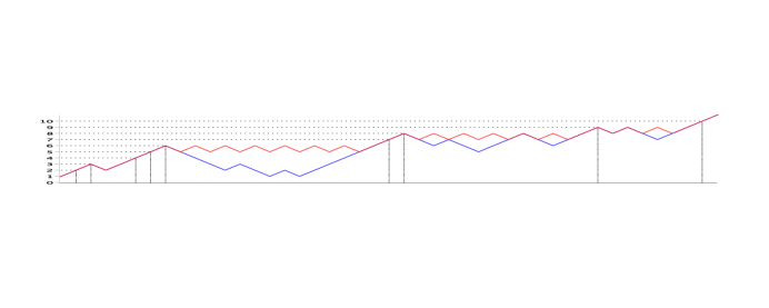
Figure 1: Portion of typical initial (blue, lower) and final (red, upper) height profiles in the F-TASEP. The vertical dotted lines are at sites in $P$.

Proof of Theorem 3.1.

For the moment we denote the set defined in (3.1) by $P_{t}$. Observe first that (2.11) implies that for fixed $i$, $h_{t}(i)$ is nondecreasing in $t$; moreover, $h_{t+1}(i)>h_{t}(i)$ is possible only if $h_{t}(i-1)>h_{t}(i)$. This implies that if $p\in P_{0}$ then for all $t\geq 0$, $h_{t}(p)=h_{0}(p)$ and $h_{t}(p)>\max_{i<p}h_{t}(i)$. Thus $p\in P_{t}$ and so $P\subset P_{t}$; since $h_{t}(p)$ takes each value in $\mathbb{Z}$ precisely once, $P_{t}=P$, verifying (a). Moreover, for any $i\in\mathbb{Z}$ there will be a $p\in P$ with $p>i$, and the upper bound $h_{t}(i)<h_{t}(p)=h_{0}(p)$ shows the existence of the limit $h_{\infty}(i)=\lim_{t\to\infty}h_{t}(i)$, and hence, via (2.9), also of the limit $\eta_{\infty}(i)$. Further, if $p$ and $p^{\prime}$ are two consecutive elements of $P$ and $p\leq i<p^{\prime}$ then $h_{\infty}(i)\geq h_{\infty}(p)-1$, since if $h_{\infty}(i)\leq h_{\infty}(p)-2$ for some $i$ with $i>p$ then necessarily $\eta_{\infty}\hbox{$(j\!:\!j+2)$}=1\,1\,0$ for some $j$ with $p<j<p^{\prime}$, and an exchange must then take place, contradicting the time-independence of $\eta_{\infty}$. The conclusion that $h_{\infty}(p)-1\leq h_{\infty}(i)\leq h_{\infty}(p)$ for $p\leq i<p^{\prime}$ yields (3.2).∎

3.2 A Bernoulli initial distribution

In this section we assume that the initial configuration $\eta_{0}$ is distributed according to the Bernoulli measure $\mu^{(\rho)}$, with $0<\rho<1/2$. Then almost every initial configuration $\eta_{0}$ satisfies (1.1); for such configurations the set $P$ of (3.1) is well defined, the analysis of the preceding section applies, and $\eta_{\infty}$ is determined as a function of $\eta_{0}$. Theorem 3.1 suggests that to obtain the distribution of $\eta_{\infty}$ we should obtain the joint distribution of the (ill-defined at the moment) “random variables” $p^{\prime}-p$ of (3.2). To state a precise result we would like to index the points of $P$, with $p_{k}<p_{k+1}$ for all $k$, but unfortunately this cannot be done without introducing some unwanted bias into the differences $p_{k+1}-p_{k}$.

To deal with this problem we first introduce the set $V:=\{\eta_{0}\mid 0\in P(\eta_{0})\}$ and let $\mu$ denote the measure $\mu^{(\rho)}$ conditioned on $V$ (we could just as well replace $V$ by $\{\eta_{0}\mid j\in P(\eta_{0})\}$ for any $j\in\mathbb{Z}$). For configurations $\eta_{0}\in V$ we label the points of $P(\eta_{0})$ so that $p_{0}=0$ and $p_{k}<p_{k+1}$. To describe the distribution of the differences $p_{k+1}-p_{k}$ under $\mu$ we will use the Catalan numbers

$$c_{n}=\frac{1}{n+1}\binom{2n}{n},\quad n=0,1,2,\ldots$$ (3.3)

(the sequence is entry A000108 in the Online Encyclopedia of Integer Sequences [20]). $c_{n}$ counts the number of strings of $n$ 0’s and $n$ 1’s in which the number of 0’s in any initial segment does not exceed the number of 1’s, or alternatively the number of Dyck paths of length $2n$: paths in the lower half plane, with possible steps $(1,1)$ and $(1,-1)$, from $(0,0)$ to $(2n,0)$.

Theorem 3.2.

The random variables $N_{k}=p_{k+1}-p_{k}$ are i.i.d. under $\mu$, with distribution

$$\mu(\{N_{k}=2n+1\})=c_{n}\rho^{n}(1-\rho)^{n+1},\quad n=0,1,2,\ldots,$$ (3.4)

Note that the independence of the variables $N_{k}$ implies that the set $P$ is a renewal point process; this is the renewal process mentioned in Section 1.

Proof of Theorem 3.2.

Whether or not a site $p$ belongs to $P$ is determined by the $\eta(i)$ with $i\leq p$, whereas given that $p\in P$, the next point $p^{\prime}$ of $P$ is determined by the $\eta(i)$ with $i>p$. This establishes the independence of the increments $N_{k}$. More specifically, if $p\in P$ and $l=p+2n+1$ then $p^{\prime}=l$ if and only if $h_{0}(l)=h_{0}(p)+1$ and $h_{0}(i)\leq h_{0}(p)$ for $p<i<l$; the latter condition holds if and only if in the string $\eta\hbox{$(p+1\!:\!l-1)$}$ the number of 0’s in any initial segment does not exceed the number of 1’s, that is, if the segment of $h_{0}(i)$ for $p\leq i<p+l$ forms a Dyck path. Thus there are $c_{n}$ configurations of $\eta\hbox{$(p+1\!:\!l)$}$ yielding $p^{\prime}=l$, and since each such configuration has probability $\rho^{n}(1-\rho)^{n+1}$, (3.4) is established. ∎

Remark 3.3.

(a) The distribution $\mu_{\infty}$ of $\eta_{\infty}$ may be expressed in terms of $\mu$ by a standard construction: $\mu_{\infty}=Z^{-1}\sum_{m\geq 0}\sum_{i=0}^{m-1}\tau_{*}^{-i}\bigl{(}\mu\big{|}_{V_{m}}\bigr{)}$, where $V_{m}=\{\eta_{0}\in V\mid p_{1}-p_{0}=m\}$ and $Z:=\sum_{m\geq 0}m\mu(V_{m})$ (compare the construction of $\Phi$ in Section 2.1).

(b) In the continuous-time Facilitated Partially Asymmetric Exclusion Process the transitions $1\,1\,0\to 1\,0\,1$ and $0\,1\,1\to 1\,0\,1$ occur at rates $p$ and $1-p$, respectively. It can be shown [1] that if this process is started in a Bernoulli measure with density $\rho<1/2$ then the final state is again described by the measure $\mu_{\infty}$ of (a), whatever the value of $p$.

We now discuss some further properties of the final state of the system, still when started from a Bernoulli measure.

Lemma 3.4.

For any $i\in\mathbb{Z}$, $\mu^{(\rho)}(\{i\in P(\eta_{0})\})=1-2\rho$.

Proof.

One can verify the result by direct consideration of the initial state, but it is easier to observe from Theorem 3.1(b) that the desired probability is just $\mu^{(\rho)}(\{\eta_{\infty}(i-1)=\eta_{\infty}(i)=0\})$, and the result then follows from $\mu^{(\rho)}(\eta_{\infty}(i-1))=\mu^{(\rho)}(\eta_{\infty}(i))=\rho$ and $\mu^{(\rho)}(\eta_{\infty}(i-1)\eta_{\infty}(i))=0$. ∎

Recall now the definitions of $V$ and $\mu$ given above; note that $\mu^{(\rho)}(V)=1-2\rho$ and that, if $\eta_{0}\in V$, then during the evolution of $\eta_{0}$ no particle can cross the bond $\langle 0,1\rangle$. This implies that $\eta_{\infty}\hbox{$(1\!:\!\infty)$}$ depends only on $\eta_{0}\hbox{$(1\!:\!\infty)$}$, and in such a manner that $\eta_{\infty}(1)=\eta_{0}(1)$ so that $\mu(\eta_{\infty}(1))=\mu^{(\rho)}(\eta_{0}(1))=\rho$.

Lemma 3.5.

For any $n\geq 1$, $\mu(\{2n\in P\})=\mu(\{2n+1\in P\})$.

Proof.

For $\eta_{0}\in V$ and $x\in\{0,1\}$ let $\eta_{0}^{x}$ be obtained by inserting $x$ into $\eta_{0}$ immediately to the right of the origin: $\eta_{0}^{x}(i)=\eta_{0}(i)$ for $i\leq 0$, $\eta_{0}^{x}(1)=x$, and $\eta_{0}^{x}(i)=\eta_{0}(i-1)$ for $i\geq 2$. We claim that $2n\in P(\eta_{0})$ iff $2n+1\in P(\eta_{0}^{0})\cap P(\eta_{0}^{1})$, which immediately implies the result. For the claim, let $h_{0}$ be the height function for $\eta_{0}$ and $h_{0}^{x}$ that for $\eta_{0}^{x}$. Note first that if $2n+1\in P(\eta_{0}^{1})$ then $2n\in P(\eta_{0})$; this is clear geometrically, since in passing from $h_{0}^{1}$ to $h_{0}$ we raise, and shift one site to the left, the portion of the height profile to the right of site 1. (An analytic proof similar to the argument given just below is easy to write down.) Next, if $2n\in P(\eta_{0})$ then similarly $2n+1\in P(\eta_{0}^{0})$. Finally, we check in more detail that if $2n\in P(\eta_{0})$ then $2n+1\in P(\eta_{0}^{1})$. We know that $h_{0}(2n)>h_{0}(i)$ for any $i<2n$ and must show that $h_{0}^{1}(2n+1)>h_{0}^{1}(i)$ for $i<2n+1$. Now if $i\geq 1$ this follows from $h_{0}^{1}(2n+1)=h_{0}(2n)-1>h_{0}(i-1)-1=h_{0}^{1}(i)$, while if $i\leq 0$ we use the fact that $h_{0}(2n)$ is even and $h_{0}(2n)>h_{0}(0)=0$ to write $h_{0}^{1}(2n+1)=h_{0}(2n)-1\geq 1>h_{0}(0)\geq h_{0}(i)=h_{0}^{1}(i)$. ∎

In stating the next theorem we let $g$ denote the two-point correlation function in the final state: $g(k)=\mu^{(\rho)}(\eta_{\infty}(0)\eta_{\infty}(k))$.

Theorem 3.6.

(a) For any $n\geq 1$, $\mu(\eta_{\infty}(2n-1))=\rho$.

(b) For any $n\geq 1$, $g(2n-1)+g(2n)=2\rho^{2}$.

Proof.

From Lemma 3.5 and the fact that $\mu^{(\rho)}(\eta_{\infty}(i)\eta_{\infty}(i+1))=0$ for any $i$ it follows that the distribution under $\mu$ of $(\eta_{\infty}(2n-1),\eta_{\infty}(2n),\eta_{\infty}(2n+1))$ is symmetric under the exchange of the first and last variables. Thus $\mu(\eta_{\infty}(2n-1))=\mu(\eta_{\infty}(2n+1))$, and this, with the observation above that $\mu(\eta_{\infty}(1))=\rho$, yields (a). But then (b) follows immediately, from

$$\mu(\eta_{\infty}(2n-1)) =\frac{1}{1-2\rho}\mu^{(\rho)}((1-\eta_{\infty}(-1))(1-\eta_{\infty}(0))\eta_{\infty}(2n-1))$$

$$=\frac{1}{1-2\rho}(\rho-g(2n)-g(2n-1)).\qed$$

An alternative proof of Theorem 3.6(a)—which, in fact, generalizes that result to $\mu(\eta_{t}(2n-1))=\rho$ for all $t$—is presented in Appendix B. Theorem 3.6(b) is then a consequence, as above. A third proof of the latter is obtained from the computation in Appendix A of the generating function for $g(k)$.

We next observe that the truncated two point function $g^{T}(k):=g(k)-\rho^{2}$ decays exponentially.

Lemma 3.7.

Let $\alpha_{0}:=(4\rho(1-\rho))^{1/2}<1$. Then for any $\alpha>\alpha_{0}$ there is a $C_{\alpha}>0$ such that $|g^{T}(k)|\leq C_{\alpha}\alpha^{k}$.

Proof sketch.

One finds the generating function $G^{T}(z):=\sum_{n=1}^{\infty}g^{T}(n)z^{n}$ and observes that it is analytic for $|z|<1/\alpha_{0}$. Some details are given in Appendix A. ∎

We next consider the variance of the number of particles in large boxes.

Theorem 3.8.

Let $S_{L}=\sum_{i=1}^{L}\eta_{\infty}(i)$ and $V_{L}=\mathop{\rm Var}(S_{L})=\mu^{(\rho)}(S_{L}^{2})-(\rho L)^{2}$. Then for $0<\rho<1/2$, $\lim_{L\to\infty}V_{L}/L=\rho(1-\rho)$.

Proof.

The exponential decay of Lemma 3.7 is amply sufficient to justify the standard formula

$$\lim_{L\to\infty}\frac{V_{L}}{L}=\rho(1-\rho)+\sum_{k=1}^{\infty}g^{T}(k).$$ (3.5)

But by Theorem 3.6, $\sum_{k=1}^{n}g^{T}(k)=0$ if $n$ is even. ∎

The result of Theorem 3.8 may also be understood in terms of the fact that, as we next discuss, a typical particle moves only a microscopic distance during the evolution. Thus the number of particles in a large box is, to high relative accuracy, the same at the end of the evolution as it was at the beginning. We will in fact show in Theorem 3.9 that the distance moved by such a typical particle has a geometric distribution with mean $\rho/(1-2\rho)$.

Consider then a particle initially located at a site $i$, with $p_{k}<i<p_{k+1}-1$, and let $i_{t}$ be its position at time $t$. During the evolution, $h_{t}(i_{t})$ will increase from $h_{0}(i)$ to $h_{0}(p_{k})-1$, so that the particle will move a distance $h_{0}(p_{k})-h_{0}(i)-1$. Now consider further the collection of all Dyck paths of length $2n$, which for the moment we think of as starting at $(0,0)$; there are $c_{n}$ such paths and each configuration described by one of them contains $n$ particles, for a total of $nc_{n}$ particles. Let $\Delta(n,d)$ be the number of these particles which will move a distance exactly $d$, and note that $\Delta(0,d)=0$. By conditioning on the site $2m$ where the path first returns to height 0 (a standard trick for obtaining the recursion for Catalan numbers) we find the recursion

$$\Delta(n,d)=\sum_{m=1}^{n}\bigl{(}c_{n-m}\Delta(m-1,d-1)+c_{m-1}\Delta(n-m,d)\bigr{)}.$$ (3.6)

This relation holds even for $d=0$ if we define $\Delta(n,-1)=c_{n}$.

Now introduce the generating functions $G(u)=\sum_{n=0}^{\infty}c_{n}u^{n}$ and $G_{d}(u)=\sum_{n=0}^{\infty}\Delta(n,d)u^{n}$ (so that $G(u)=G_{-1}(u)$). It is well-known [17] that $G(u)$ satisfies $G(u)=1+uG(u)^{2}$ and that explicitly $G(u)=2/(1+\sqrt{1-4u})$. From (3.6) we have $G_{d}(u)=uG(u)(G_{d-1}(u)+G_{d}(u))$, easily solved to give

$$G_{d}(u)=G(u)(G(u)-1)^{d+1}.$$ (3.7)

We next condition on there being a particle at the origin in $\eta_{0}$, let $D$ be the distance that that particle moves, and find the distribution of $D$. For some $k$ we will have $p_{k}<0<p_{k+1}$; we first calculate the probability $\pi_{n}$ that $p_{k+1}-p_{k}=2n+1$. In that event there are $n$ possible sites for $p_{k}$, the probability that a selected site lies in $P(\eta_{0})$ is $(1-2\rho)$ (Lemma 3.4), and we must divide by $\rho$ to condition on $\eta_{0}(0)=1$, so that from (3.4),

$$\pi_{n}=n(1-2\rho)c_{n}\rho^{n-1}(1-\rho)^{n+1}.$$ (3.8)

But since, given that $p_{k+1}-p_{k}=2n+1$, all compatible Dyck paths and positions of the origin relative to the path are equally likely,

$$\mu^{(\rho)}(D=d\mid\eta_{0}=1) =\sum_{n=1}^{\infty}\pi_{n}\frac{\Delta(n,d)}{nc_{n}}$$

$$=\frac{(1-\rho)(1-2\rho)}{\rho}G_{d}(\rho(1-\rho))$$

$$=\frac{1-2\rho}{1-\rho}\left(\frac{\rho}{1-\rho}\right)^{d}.$$ (3.9)

We have proved:

Theorem 3.9.

The distance $D$ moved by a “typical” particle, i.e., by the particle at the origin given that at time zero there is such a particle, has geometric distribution, with ratio $\rho/(1-\rho)$ and mean $\rho/(1-2\rho)$.

Remark 3.10.

Consider the deterministic discrete-time TASEP, in which all particles with an empty site to their left jump to that site at integer times. (We have reversed the conventional choice of jump direction, with which the model is also called CA 184 [4], for reasons to be seen shortly.) The model is often studied in a probabilistic version, in which each jump takes place with some probability $p$; in this case there is a unique TIS state [7]. For the deterministic model with density $\rho<1/2$, however, any TI state in which, with probability 1, each particle is isolated, is stationary, since each configuration simply translates to the left with velocity 1. These are all the TIS measures [4]. It is then natural to consider a modified dynamics in which, at each time step, one first does a TASEP update, then translates all particles to the right by one site. This gives a modification of the facilitated dynamics: an isolated particle does not move, but if there is a block of $k$ particles then the left-most one stays fixed and the remaining $k-1$ move one step to the right. Our analysis of the F-TASEP through the height function can then be applied directly, so that an initial configuration $\eta_{0}$ evolves under the modified TASEP dynamics to the same $\eta_{\infty}$ as in the F-TASEP.

For TI initial (and hence final) states the modification of the dynamics will not affect stationarity, so that if we start the system in some TI measure $\lambda$ then the final measure will be the F-TASEP final measure $\lambda_{\infty}$; in particular, if $\lambda$ is Bernoulli then the final measure will be the one of Remark 3.3. On the other hand, if $\lambda$ is the initial measure for the TASEP in which particles move to the right then the final measure will be $R_{*}((R_{*}\mu)_{\infty})$, where $R:X\to X$ is reflection. For either direction of motion, stationary states at $\rho>1/2$ may then be determined through the usual particle-hole symmetry.

4 The high density region

We now turn to the high density region $2/3<\rho<1$; we will be brief, because the behavior of the model here is very similar to that in the low density region. Recall from Sections 2 and 2.3 that the dynamics will now be given by $\eta_{t+1}=U^{(h)}\eta_{t}$ and $h_{t+1}=U^{(h)}h_{t}$.

Let us first fix an initial configuration $\eta_{0}$ with density $\rho$, $2/3<\rho<1$, and determine its final form $\eta_{\infty}$. We define $Q:=\{q\in\mathbb{Z}\mid h_{t}^{*}(q)<\inf_{i<q}h_{t}^{*}(i)\}$; Theorem 4.1(a) below justifies this notation, which ignores the apparent $t$ dependence of $Q$. Since $h_{t}$ has mean slope $1-2\rho<-1/3$, $\lim_{i\to\pm\infty}h^{*}_{t}(i)=\mp\infty$, so that $Q$ is well defined and unbounded above and below. Note that if $q\in Q$ then $\eta\hbox{$(q-2\!:\!q)$}=1\,1\,1$ for all $k$.

Theorem 4.1.

(a) $Q$ as defined above is independent of $t$.

(b) For each $i\in\mathbb{Z}$, $\eta_{t}(i)$ and $h_{t}(i)$ are eventually constant, and if we denote these limiting values by $\eta_{\infty}(i)$ and $h_{\infty}(i)$, then then for $q$ and $q^{\prime}$ any consecutive points of $Q$ there is an $n$ with

$$\eta_{\infty}\hbox{$(q+1\!:\!q^{\prime})$}=(0\,1\,1)^{n}d\,1.$$ (4.1)

Proof.

The proof is completely parallel to that of Theorem 3.1. One first checks that, for $i\in\mathbb{Z}$, $h^{*}_{t}(i)$ is nonincreasing in $t$, with $h^{*}_{t+1}(i)<h^{*}_{t}(i)$ possible only if $h^{*}_{t}(k-1)>h^{*}_{t}(k)$; this implies that $Q$ is time-independent and that the $h^{*}_{\infty}$, and hence $h_{\infty}$ and $\eta_{\infty}$, exist. Then the fact that $\eta_{\infty}\in X^{(h)}$ (see Corollary 2.3(c)) yields (4.1). ∎

Now we suppose that the initial configuration $\eta_{0}$ is distributed according to the Bernoulli measure $\mu^{(\rho)}$, with $\rho$ satisfying $2/3<\rho<1$. Let $V^{*}:=\{\eta_{0}\mid 0\in Q(\eta_{0})\}$, let $\mu^{*}$ denote the measure $\mu^{(\rho)}$ conditioned on $V^{*}$, and for $\eta_{0}\in Q$ index the points of $Q$ in increasing order, with $q_{0}=0$. We first find the distribution of the differences $q_{k}-q_{k-1}$, and in doing so will refer to the sequence

$$d_{n}=\frac{1}{2n+1}\binom{3n}{n},\qquad n=0,1,2,\ldots.$$ (4.2)

The $d_{n}$ are a particular case of Fuss-Catalan or Raney numbers [15] (OEIS entry A001764 [20]). $d_{n}$ counts the number of paths from the origin to $(3n,-n)$, with possible steps $(1,1)$ and $(1,-1)$, such that the path never goes below the line $y=-x/3$.

Theorem 4.2.

The random variables $N^{*}_{k}=q_{k+1}-q_{k}$ are i.i.d. under $\mu^{*}$, with distribution

$$\mu^{*}\{N^{*}_{k}=3n+1\}=d_{n}\rho^{2n+1}(1-\rho)^{n},\quad n=0,1,2,\ldots,$$ (4.3)

Proof.

Independence of the increments $N^{*}_{k}$ is established as in the proof of Theorem 3.2. As in that proof, if $l=q_{k}+3n+1$ then $q_{k+1}=l$ if and only if $h^{*}_{0}(l)=h^{*}_{0}(q_{k})-2/3$ and the segment of $h_{0}(i)$ for $q_{k}\leq i<q_{k}+l$ is a path of the type counted by $d_{n}$ (see the previous paragraph). Thus there are $d_{n}$ configurations of $\eta\hbox{$(q_{k}+1\!:\!l)$}$ yielding $q_{k+1}=l$, each with probability $\rho^{2n+1}(1-\rho)^{n}$, establishing (3.4). ∎

Our next theorem summarizes various results for the high density region which are parallel to the results of Section 3 for the low density region. In stating these we define, as in Section 3, $g(k)=\mu^{(\rho)}(\eta_{\infty}(0)\eta_{\infty}(k))$. We omit the proofs, all of which are modifications of those of the previous section.

Theorem 4.3.

Suppose that $2/3<\rho<1$. Then:

(a) For any $i\in\mathbb{Z}$, $\mu^{(\rho)}(\{i\in Q(\eta_{0})\})=3\rho-2$.

(b) For any $n\geq 1$, $\mu^{*}(\{3n\in Q\})=\mu^{*}(\{3n+1\in Q\})$.

(c) For any $n\geq 0$, $\mu^{*}(\{\eta_{\infty}(3n+1)=1\})=\rho$.

(d) For any $n\geq 1$, $g(3n-2)+g(3n-1)+g(3n)=3\rho^{2}$.

(e) Let $\alpha^{*}_{0}:=(27\rho^{2}(1-\rho)/4d)^{1/3}<1$. Then for any $\alpha^{*}>\alpha^{*}_{0}$ there is a $C_{\alpha^{*}}>0$ such that $|g^{T}(k)|\leq C_{\alpha^{*}}\alpha^{*k}$.

(f) Let $S_{L}=\sum_{i=1}^{L}\eta_{\infty}(i)$ and $V_{L}=\mathop{\rm Var}(S_{L})=\mu^{(\rho)}(S_{L}^{2})-(\rho L)^{2}$. Then for $2/3<\rho<1$, $\lim_{L\to\infty}V_{L}/L=\rho(1-\rho)$.

There is no analogue of Theorem 3.9, since in the high density region particles never stop moving, either in the original dynamics given by $U$ or the modified dynamics given by $U^{(h)}$.

5 The intermediate density region

In this section we study the dynamics in the intermediate density region $1/2<\rho<2/3$.

5.1 Evolution of a single configuration

We first discuss the evolution of a given configuration of density $\rho$, beginning with some preliminary technical results. Recall that in each of Sections 3 and 4 the final configuration was determined by a special family of sites; these families were denoted $P$ and $Q$ respectively, and were stationary during the evolution. In the intermediate region we need to define, somewhat similarly, two families of sites, which we will denote by $P=\{p_{k}\}_{k\in\mathbb{Z}}$ and $Q=\{q_{k}\}_{k\in\mathbb{Z}}$; here, however, the sites in these families move during the evolution.

Definition 5.1.

Suppose that we are given a height profile $h(i)$, $i\in\mathbb{Z}$, corresponding via (2.9) to a configuration $\eta$ of density $\rho$, $1/2<\rho<2/3$; as usual we let $h^{*}(i)=h(i)+i/3$. Let $A,B\,\bigl{(}=A(\eta),B(\eta)\bigr{)}\subset\mathbb{Z}$ be the sets of those sites which satisfy respectively

$$h(a)>\sup_{r>a}h(r),\ a\in A,\qquad\hbox{and}\qquad h^{*}(b)<\inf_{r>b}h^{*}(r),\ b\in B.$$ (5.1)

$A$ and $B$ are disjoint, since if $r\in A\cap B$ then (5.1) implies that $h(r)>h(r+1)>h(r)-1/3$, impossible since $h$ takes integer values. Moreover, $A$ and $B$ are unbounded, both above and below, by our assumption on $\rho$; we index the points of $A$ and $B$ as increasing sequences $(a_{j})_{j\in\mathbb{Z}}$ and $(b_{j})_{j\in\mathbb{Z}}$, respectively. Let $P$ be the set of elements $a_{j}\in A$ such that there exists a $b\in B$ satisfying $a_{j-1}<b<a_{j}$, and similarly let $Q$ be the set of $b_{j}\in B$ such that there exists an $a\in A$ satisfying $b_{j-1}<a<b_{j}$. If we index $P$ as the increasing sequence $(p_{k})_{k\in\mathbb{Z}}$, then clearly exactly one point of $Q$—the smallest element of $B\cap(p_{k-1},p_{k})$—lies in $(p_{k-1},p_{k})$. We denote this element $q_{k-1}$.

Lemma 5.2.

The sequences $p=(p_{k})_{k\in\mathbb{Z}}$ and $q=(q_{k})_{k\in\mathbb{Z}}$ satisfy

$$\cdots p_{-1}<q_{-1}<p_{0}<q_{0}<p_{1}<q_{1}\cdots$$ (5.2)

and

$$h(p_{k}) >\sup_{r>p_{k}}h(r),$$ (5.3)

$$h(p_{k}) \geq\sup_{q_{k-1}\leq r\leq p_{k}}h(r),$$ (5.4)

$$h^{*}(q_{k}) <\inf_{r>q_{k}}h^{*}(r),$$ (5.5)

$$h^{*}(q_{k}) \leq\inf_{p_{k}\leq r\leq q_{k}}h^{*}(r).$$ (5.6)

Moreover they are, up to a shift of labels, the unique sequences satisfying these equations.

A graphical interpretation of (5.3)–(5.6) is given in Figure 2, drawn for future purposes at time 0. Here $h=h_{0}$ is represented as the piecewise linear curve obtained by connecting each pair of points $(k,h(k))$ and $(k+1,h(k+1))$ by a line segment. We have introduced also two families of straight lines: for each $k\in\mathbb{Z}$, $L_{k}$ is a horizontal line through $(p_{0,k},h_{0}(p_{0,k}))$, and $L_{k}^{*}$ a line of slope $-1/3$ through $(q_{0,k},h_{0}(q_{0,k}))$. (5.3) and (5.4) imply respectively that the profile must lie below $L_{k}$ between $q_{k-1}$ and $p_{k}$ and strictly below $L_{k}$ to the right of $p_{k}$. Similarly, (5.5) and (5.6) imply that the profile lies above $L_{k}^{*}$ between $p_{k}$ and $q_{k}$ and strictly above $L_{k}^{*}$ to the right of $q_{k}$.

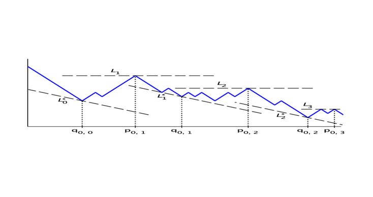
Figure 2: Portion of typical initial height profile $h_{0}$ (solid blue line), with the initial $p_{k}$ and $q_{k}$ values and the lines $L_{k}$ and $L_{k}^{*}$.

Proof of Lemma 5.2.

$(p_{k})$ and $(q_{k})$ clearly satisfy (5.2), (5.3), and (5.5). (5.4) follows immediately from the fact that there can be no point of $A$ between $q_{k-1}$ and $p_{k}$; the proof of (5.6) is similar.

For uniqueness, suppose that $(\hat{p}_{k})_{k\in\mathbb{Z}}$ and $(\hat{q}_{k})_{k\in\mathbb{Z}}$ satisfy (5.2)–(5.6), and let $\widehat{P}=\{\hat{p}_{k}\mid k\in\mathbb{Z}$} and $\widehat{Q}=\{\hat{q}_{k}\mid k\in\mathbb{Z}$}. From (5.3) and (5.5) we see that $\widehat{P}\subset A$ and $\widehat{Q}\subset B$. Now note that, for any $k$, (5.4) implies that no point of $A$ can belong to $(\hat{q}_{k-1},\hat{p}_{k})$; this immediately yields $\hat{p}_{k}\in P$. Similarly, (5.6) implies that $\hat{q}_{k}\in Q$, so that $\widehat{P}\subset P$ and $\widehat{Q}\subset Q$. But now we may again use $A\cap(\hat{q}_{k-1},\hat{p}_{k})=\emptyset$ to conclude that no point of $P$, and hence by (5.2) no point of $Q$, can lie in $(\hat{q}_{k-1},\hat{p}_{k})$; similarly, no point of $P$ or $Q$ can lie in $(\hat{p}_{k},\hat{q}_{k})$, so that $P=\hat{P}$ and $Q=\hat{Q}$. ∎

In our next result we record some trivial consequences of Lemma 5.2.

Lemma 5.3.

If $p$ and $q$ are as in Lemma 5.2 then for any $k\in\mathbb{Z}$ we have (a) $h^{*}(p_{k}+2)=h^{*}(p_{k})-4/3$, (b) $h(q_{k}+1)=h(q_{k})+1$, (c) $h^{*}(q_{k})\leq h^{*}(p_{k}+2)$, and (d) $h(p_{k+1})\geq h(q_{k}+1)$.

Proof.

Observe first that $\eta(p_{k}+1)=\eta(p_{k}+2)=1$, for otherwise $h(p_{k}+2)\geq h(p_{k})$, contradicting (5.3); this gives (a). Similarly, $\eta(q_{k}+1)=0$, since otherwise $h^{*}(q_{k}+1)<h^{*}(q_{k})$, contradicting (5.5), and this implies (b). (c) is an immediate consequence of (5.5) and (5.6), and (d) of (5.4).∎

We now turn to the dynamics. We fix an initial configuration $\eta_{0}$, with density $\rho$ satisfying $1/2<\rho<2/3$ (see (1.1)); this then evolves via $\eta_{t+1}=U^{(i)}\eta_{t}$ and $h_{t+1}=U^{(i)}h_{t}$. Let $A_{t}$, $B_{t}$, $P_{t}$, $Q_{t}$, $a_{t}$, $b_{t}$, $p_{t}$ and $q_{t}$ denote the sets and sequences obtained from $h_{t}$ as in the definitions above.

Remark 5.4.

Before giving any further proofs we give a brief qualitative description of the evolution of $h_{t}$; a key role is played by the lines $L_{k}$, $L_{k}^{*}$ of Figure 2. During the evolution, the point $(p_{t,k},h(p_{t,k}))$ travels to the left along $L_{k}$, moving either zero or two lattice sites at each time step and stopping just short of the intersection with $L_{k}^{*}$. Similarly, $(q_{t,k},h_{t}(q_{t,k}))$ travels up and to the left along $L_{k}^{*}$, zero or three lattice sites at each time step, and stops just short of intersection with $L_{k+1}$ ($h^{*}_{t}(q_{t,k})$ is constant during this evolution). The precise limiting values $p_{\infty,k}$ and $q_{\infty,k}$ are given in (5.13) and (5.14) below. After these special points have reached their limiting positions the profile may continue to evolve between them, eventually reaching a limiting position everywhere. In the region between $p_{\infty,k}$ and $q_{\infty,k}$, the limiting configuration has the form $0\,1\,1\,0\,1\,1\,\cdots$ and $h_{\infty}$ has average slope $-1/3$, while between $q_{\infty,k-1}$ and $p_{\infty,k}$ the form is $1\,0\,1\,0\,\cdots$ and $h_{\infty}$ is essentially flat. The limiting configuration for the initial condition of Figure 2 is shown in Figure 3.

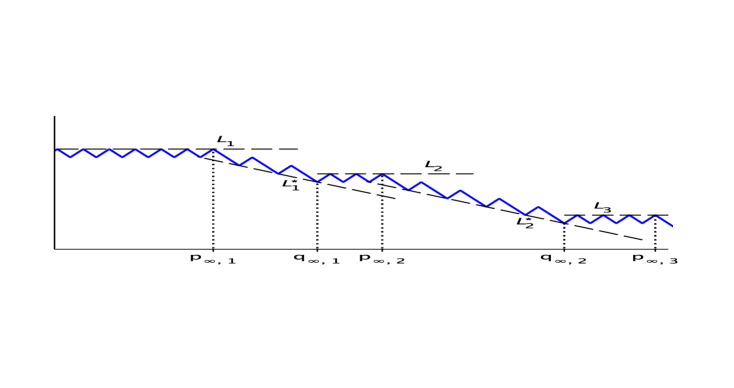
Figure 3: Portion of final height profile for the initial profile of Figure 2, with the final $p_{k}$ and $q_{k}$ values.

Next we show that (with appropriate indexing) the points $(p_{t,k},h_{t}(p_{t,k}))$ and $(q_{t,k},h_{t}^{*}(q_{t,k}))$ move during the evolution as described in Remark 5.4.

Lemma 5.5.

The sequences $p_{t}$ and $q_{t}$ may be indexed so that for all $t\geq 0$,

$$(p_{t+1,k},h_{t+1}(p_{t+1,k})) =(p_{t,k},h_{t}({p_{t},k}))\text{ or }(p_{t,k}-2,h_{t}({p_{t},k})),$$ (5.7)

$$(q_{t+1,k},h_{t+1}^{*}(q_{t+1,k})) =(q_{t,k},h_{t}^{*}({q_{t},k}))\text{ or }(q_{t,k}-3,h_{t}^{*}({q_{t},k})).$$ (5.8)

In particular, for each $k\in\mathbb{Z}$ the sequences $(p_{t,k})_{t=0}^{\infty}$ and $(q_{t,k})_{t=0}^{\infty}$ are nonincreasing and the sequences $(h_{t}(p_{t,k}))_{t=0}^{\infty}$ and $(h_{t}^{*}(q_{t,k}))_{t=0}^{\infty}$ constant.

Proof.

Examination of the action of the dynamics near the $p_{k}$ and $q_{k}$ suggests that appropriate indexing will yield $p_{t+1,k}=p^{\prime}_{k}$ and $q_{t+1,k}=q^{\prime}_{k}$, where

$$p^{\prime}_{k} =\begin{cases}p_{t,k},&\text{if $\eta_{t}\hbox{$(p_{t,k}+1\!:\!p_{t,k}+3)$}=1\,1\,0$,}\\ p_{t,k}-2,&\text{if $\eta_{t}\hbox{$(p_{t,k}+1\!:\!p_{t,k}+3)$}=1\,1\,1$,}\end{cases}$$ (5.9)

$$q^{\prime}_{k} =\begin{cases}q_{t,k},&\text{if $\eta_{t}\hbox{$(q_{t,k}+1\!:\!q_{t,k}+3)$}=0\,1$,}\\ q_{t,k}-3,&\text{if $\eta_{t}\hbox{$(q_{t,k}+1\!:\!q_{t,k}+3)$}=0\,0$,}\end{cases}$$ (5.10)

(in each case the given possibilities are exhaustive). To verify this, and hence prove the result (for one sees easily that $h_{t+1}(p_{k}^{\prime})=h_{t}(p_{t,k})$ and $h_{t+1}^{*}(q_{k}^{\prime})=h_{t}^{*}(q_{t,k})$) it suffices, by the uniqueness in Lemma 5.2, to check that $(p_{k}^{\prime})$ and $(q_{k}^{\prime})$ satisfy (5.2)–(5.6).

Now (5.2)–(5.6) imply that if $p^{\prime}_{k}=p_{t,k}-2$ then either $q_{k-1}^{\prime}=q_{t,k-1}-3$ or $q_{t,k-1}\leq p_{t,k}-3$, and that if $q_{k}^{\prime}=q_{t,k}-3$ then either $p_{t,k}\leq q_{t,k}-4$ or $p_{t,k}=q_{t,k}-3$ but $p^{\prime}_{k}=p_{t,k}-2$; (5.2) for $(p_{k}^{\prime})$ and $(q_{k}^{\prime})$ follows. To continue, recall that the $U^{(i)}$ dynamics takes place in two steps, with the usual F-TASEP dynamics, at which let us say $h_{t}(i)$ becomes $H(i)$, followed by a two-site translation to the left (we also write $H^{*}(i)=H(i)+i/3$). Now for $i>p_{t,k}$, $H(i)\leq h_{t}(p_{t,k})$, with equality only if $i=p_{t,k}+2$ and $\eta_{t}\hbox{$(p_{t,k}+1\!:\!p_{t,k}+3)$}=1\,1\,0$, and it is precisely in this case that $i$ becomes $p^{\prime}_{k}$ after the translation. Thus (5.3) is satisfied for $p_{k}^{\prime}$. (5.5) for $q_{k}^{\prime}$ is checked similarly.

One can check (5.4) and (5.6) considering separately the various cases of (5.9) and (5.10). To illustrate, consider (5.6) when $p_{k}^{\prime}=p_{t,k}-2$ and $q_{k}^{\prime}=q_{t,k}$. If $p_{t,k}\leq i\leq q_{t,k}$ and $h^{*}_{t}(i)=h^{*}(q_{t,k})$ then from (5.6) at time $t$ necessarily $\eta\hbox{$(i-1\!:\!i+1)$}=1\,1\,0$, so that $H^{*}(i)=h^{*}_{t}(i)+2$, and this with (5.5) implies that $H^{*}(i)\geq h_{t}^{*}(q_{t,k})+2/3$ for $p_{t,k}\leq i\leq q_{t,k}+2$. After the translation step this becomes $H^{*}(i)\geq h_{t}^{*}(q_{t,k})$ for $p_{k}^{\prime}\leq i\leq q_{k}^{\prime}$, verifying (5.6) in this case. ∎

Theorem 5.6.

For each $i,k\in\mathbb{Z}$, $\eta_{t}(i)$, $h_{t}(i)$, $p_{t,k}$, and $q_{t,k}$ are eventually constant. If we denote these limiting values by $\eta_{\infty}(i)$, $h_{\infty}(i)$, $p_{\infty,k}$, and $q_{\infty,k}$, then $p_{\infty}$ and $q_{\infty}$ are the sequences obtained from $h_{\infty}$ as in Definition 5.1, and $\eta_{\infty}$ is given by

$$\eta_{\infty}\hbox{$(q_{\infty,k-1}+1\!:\!p_{\infty,k})$}=0\,1\,0\,1\,\ldots 0\,1\,0,$$ (5.11)

$$\eta_{\infty}\hbox{$(p_{\infty,k}+1\!:\!q_{\infty,k})$}=1\,1\,0\,1\,1\,\ldots 0\,1\,1.$$ (5.12)

Moreover,

$$p_{\infty,k} =q_{0,k}-3(h_{0}(p_{0,k})-h_{0}(q_{0,k}))+4,$$ (5.13)

$$q_{\infty,k} =p_{0,k+1}-3(h_{0}^{*}(p_{0,k+1})-h_{0}^{*}(q_{0,k}))+3.$$ (5.14)

We can summarize the theorem thus: the final configuration $\eta_{\infty}$ has the form

$$\eta_{\infty}=\cdots(0\,1)^{n_{k}}(0\,1\,1)^{m_{k}}(0\,1)^{n_{k+1}}(0\,1\,1)^{m_{k+1}}\cdots,$$ (5.15)

with

$$2n_{k} =p_{\infty,k}-q_{\infty,k-1}-1=3(h_{0}^{*}(q_{0,k})-h_{0}^{*}(q_{0,k-1})),$$ (5.16)

$$3m_{k} =q_{\infty,k}-p_{\infty,k}+1=3(h_{0}(p_{0,k+1})-h_{0}(p_{0,k})).$$

These results are illustrated in Figure 4.

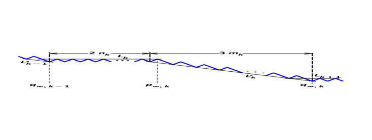
Figure 4: Illustration of equations (5.11), (5.12), and (5.15).

Proof of Theorem 5.6.

The nonincreasing sequences $(p_{t,k})_{t=0}^{\infty}$ and $(q_{t,k})_{t=0}^{\infty}$ are clearly bounded below, since, for example, $\bigl{(}q_{t,k},h_{t}(q_{t,k})\bigr{)}$ must remain on the line $L_{k}^{*}$, and by (5.4) must stay below $L_{k}$. Thus the limits $p_{\infty,k}$ and $q_{\infty,k}$ exist and will be attained by some finite time. Suppose that $t$ is a time for which $q_{t,k-1}$, $p_{t,k}$, and $q_{t,k}$ have reached their limiting values.

To establish (5.11), note first that if $\eta_{t}$ satisfies (5.11) then this will remain true as $t$ increases. Moreover, if (5.11) does not hold (for $\eta_{t}$) then by (5.4) we just have that

$$\eta_{t}\hbox{$(q_{\infty,k-1}+1\!:\!p_{\infty,k}+3)$}=\cdots\,0\,0\,(10)^{j}\,1\,1\,0$$ (5.17)

for some $j\geq 0$. But then $\eta_{t+1}$ must either satisfy (5.11) or be of the form (5.17) with $j$ replaced by some $j^{\prime}\geq j+1$. Thus (5.11) must be attained in finite time. (5.12) is obtained similarly, with (5.17) replaced by

$$\eta_{t}\hbox{$(p_{\infty,k}+1\!:\!q_{\infty,k}+2)$}=\cdots\,1\,1\,1\,(011)^{j}\,0\,1.$$ (5.18)

Finally, it follows from (5.11) that $q_{\infty,k}=i+3$, where $i$ is the site at which the lines $L^{*}_{k-1}$ and $L_{k}$ intersect, and this is just (5.14). Similarly, (5.12) implies that $p_{\infty,k}=i^{\prime}+4$, with $i^{\prime}$ is the intersection of $L_{k}$ and $L^{*}_{k}$, yielding (5.13). ∎

5.2 An initial Bernoulli distribution

We again take up the case in which the initial configuration $\eta_{0}$ is distributed according to the Bernoulli measure $\mu^{(\rho)}$, now with $1/2<\rho<2/3$, and ask for the distribution of the final configuration $\eta_{\infty}$, which we will obtain from the joint distribution of the random variables $n_{k}$ and $m_{k}$ of (5.15) (once these are precisely defined—compare Theorem 3.2). Note that these variables are expressed in (5.16) as functions of the initial configuration; we will hence in this section refer to properties of the initial configuration only, and write simply $\eta$, $h$, $p_{k}$, and $q_{k}$ rather than $\eta_{0}$, etc. While the process $\ldots,n_{k},m_{k},n_{k+1}\ldots$ is not Markovian, we will show that one may define a “hidden” Markov process, determined by the initial configuration, such that the variables $n_{k}$ and $m_{k}$ are functions of the variables of that process.

To obtain a well-defined labeling of the points of $P$ and $Q$ we introduce $V:=\{\eta\in X_{\rho}\mid 0\in P(\eta)\}$, defining $p_{0}(\eta)=0$ for $\eta\in V$ and labeling the remaining points of $P(\eta)$ and $Q(\eta)$ to satisfy (5.2). We write $\mu$ for the measure $\mu^{(\rho)}$ conditioned on $V$. We also decompose $X_{\rho}$ as $X_{\rho}=X_{\rho}^{-}\times X_{\rho}^{+}$, where $X_{\rho}^{-}\subset\{0,1\}^{\mathbb{Z}_{-}}$ is the set of configurations $\alpha:\mathbb{Z}_{-}\to\{0,1\}$ which satisfy $\lim_{N\to\infty}(N+1)^{-1}\sum_{i=-N}^{0}\alpha(i)=\rho$, and $X_{\rho}^{+}\subset\{0,1\}^{\mathbb{N}}$ is the set of configurations $\beta:\mathbb{N}\to\{0,1\}$ which satisfy $\lim_{N\to\infty}N^{-1}\sum_{i=1}^{N}\beta(i)=\rho$. We correspondingly write $\eta\in X_{\rho}$ as $(\eta^{-},\eta^{+})$.

Now suppose that $F\subset V$ is an event, with $\mu(F)>0$, specifying an arbitrary amount of information about $\eta^{-}$ and the $p_{k}$, $h(p_{k})$, $q_{k}$, and $h(q_{k})$ for $k<0$, including in particular the values of $q_{-1}=\tilde{q}$ and $h^{*}(q_{-1})=\tilde{h}^{*}$, while $F_{0}\subset V$ specifies only $q_{-1}=\tilde{q}$ and $h^{*}(q_{-1})=\tilde{h}^{*}$ (note that the nonlocality in Definition 5.1 means that $\eta^{-}$ does not determine the $p_{k}$ and $q_{k}$, $k<0$). Clearly from (5.3) and (5.5), and the fact that $p_{0}=h(p_{0})=0$ on $V$, the occurrence of either $F$ or $F_{0}$ implies that $I$ occurs, where

$$I\,(=I_{\tilde{h}^{*}}):=\{\eta\mid h(i)<0\text{ and }h^{*}(i)>\tilde{h}^{*}\text{ for all $i\geq 1$}\}.$$ (5.19)

The next result gives the basic Markovian property of the $p_{k}$’s and $q_{k}$’s.

Lemma 5.7.

The distribution of $\eta^{+}$ when conditioned on $F$ is the same as when conditioned on $F_{0}$. Moreover, this distribution is explicitly given by the marginal of $\mu^{(\rho)}$ on $X_{\rho}^{+}$, conditioned on $I$.

In preparation for the proof we make a preliminary definition: for $\alpha\in X_{\rho}^{-}$ we adapt Definition 5.1 to define $A^{\prime}(\alpha):=\{a\leq 0\mid h(a)>\sup_{a<r\leq 0}h(r)\}$, $B^{\prime}(\alpha):=\{b<0\mid h^{*}(b)<\inf_{b<r\leq 0}h^{*}(r)\}$ (so that $0\in A^{\prime}(\alpha)$, $0\notin B^{\prime}(\alpha)$) and obtain $P^{\prime}(\alpha)$ and $Q^{\prime}(\alpha)$ from $A^{\prime}(\alpha)$ and $B^{\prime}(\alpha)$ in parallel with Definition 5.1; we index the elements of these sets as $(p^{\prime}_{k})_{k\leq 0}$ and $(q^{\prime}_{k})_{k<0}$, with $p_{0}^{\prime}=\max P^{\prime}(\alpha)$. We view $P^{\prime}(\eta^{-})$ and $Q^{\prime}(\eta^{-})$ as approximations to $P(\eta)\cap\mathbb{Z}_{-}$ and $Q(\eta)\cap\mathbb{Z}-$ which depend only on $\eta^{-}$. But we have

Lemma 5.8.

If $\eta\in V$ then $P^{\prime}(\eta^{-})=P(\eta)\cap\mathbb{Z}_{-}$ and $Q^{\prime}(\eta^{-})=Q(\eta)\cap\mathbb{Z}_{-}$.

Proof.

Clearly $B(\eta)\subset B^{\prime}(\eta^{-})$ for all $\eta\in X$ and if $\eta\in V$ then $A^{\prime}(\eta^{-})=A(\eta)$. We index the points of $A(\eta)$ and $A^{\prime}(\eta^{-})$ so that $a_{0}=a^{\prime}_{0}=0$. Then $q_{-1}(\eta)=\min\bigl{(}B(\eta)\cap(a_{-1},a_{0})\bigr{)}$ and since, by (5.6), $h^{*}(r)\geq h^{*}(q_{-1})$ for $a_{-1}\leq r<q_{-1}$, $B^{\prime}(\eta^{-})\cap(a_{-1},q_{-1})=\emptyset$. From this we find easily that $B^{\prime}(\eta^{-})\cap(-\infty,q_{-1}]=B(\eta)\cap(-\infty,q_{-1}]$ and the result follows.∎

Proof of Lemma 5.7.

Without loss of generality we may assume that $F$ has the form $V\cap G_{L}\cap H_{N}$, where $G_{L}$ specifies $\eta(i)$ for $-L\leq i\leq 0$ and $H_{N}$ specifies $(p_{k},h(p_{k}))$ for $-N\leq k\leq 0$ and $(q_{k},h^{*}(q_{k}))$ for $-N\leq k<0$, and in particular requires that $p_{0}=h(p_{0})=0$, $q_{-1}=\tilde{q}$, and $h(q_{-1})=\tilde{h}^{*}$. We claim that $F=G_{L}\cap H_{N}^{\prime}\cap I$, where $H^{\prime}_{N}$ gives the same specification to the $p^{\prime}_{k}(\eta^{-})$ and $q^{\prime}_{k}(\eta^{-})$ that $H_{N}$ gave to the $p_{k}$ and $q_{k}$. Assuming this, for $J$ an arbitrary event depending only on $\eta(i)$ for $i\geq 1$ we have, using first $F\subset V$ and then $\mu^{(\rho)}(F)=\mu^{(\rho)}(G_{L}\cap H^{\prime}_{N})\mu^{(\rho)}(I)$ and $\mu^{(\rho)}(J\cap F)=\mu^{(\rho)}(G_{L}\cap H^{\prime}_{N})\mu^{(\rho)}(J\cap I)$,

$$\mu(J\mid F)=\mu^{(\rho)}(J\mid F)=\mu^{(\rho)}(J\mid I),$$ (5.20)

which is the desired conclusion.

To verify that $F=G_{L}\cap H_{N}^{\prime}\cap I$ we observe first that if $\eta\in F$ then (5.3) and (5.5) imply that $\eta\in I$; moreover, by Lemma 5.8, $\eta\in H_{N}^{\prime}$; thus $F\subset G_{L}\cap H_{N}^{\prime}\cap I$. Conversely, if $\eta\in G_{L}\cap H_{N}^{\prime}\cap I$ then $\eta\in I$ implies that $0\in A(\eta)$ and, with $\tilde{q}\in B^{\prime}(\eta^{-})$, that $\tilde{q}\in B(\eta)$. Moreover, from $\eta\in H_{N}^{\prime}$ it follows that $0\in P^{\prime}(\eta^{-})$, and with $\eta\in I$ and $\tilde{q}\in Q^{\prime}(\eta^{-})$ this implies that $\eta\in V$; from this, $G_{L}\cap H_{N}^{\prime}\cap I\subset F$ is immediate. ∎

A similar result holds with the roles of the $p_{k}$ and $q_{k}$ interchanged. Let $V^{*}:=\{\eta\in X_{\rho}\mid 0\in Q(\eta)\}$, index the points of $P$ and $Q$ on $V^{*}$ via $q_{0}(\eta)=0$ and (5.2), and let $\mu^{*}$ be $\mu^{(\rho)}$ conditioned on $V^{*}$. Suppose that $F^{*}\subset V^{*}$ is an event, with $\mu(F^{*})>0$, specifying an arbitrary amount of information about $\eta^{-}$ and the $p_{k}$, $h(p_{k})$, $q_{k}$, and $h(q_{k})$ for $k<0$, including in particular the values of $p_{-1}=\hat{p}$ and $h(p_{-1})=\hat{h}$, while $F_{0}^{*}\subset V$ specifies only $p_{-1}=\hat{p}$ and $h(p_{-1})=\hat{h}$. The occurrence of either $F^{*}$ or $F_{0}^{*}$ implies that $I^{*}$ occurs, where

$$I^{*}\,(=I^{*}_{\hat{h}}):=\{\eta\mid h^{*}(i)>0\text{ and }h(i)<\hat{h}\text{ for all $i\geq 1$}\}.$$ (5.21)

The proof of the next result is parallel to that of Lemma 5.7.

Lemma 5.9.

The distribution of $\eta^{+}$ when conditioned on $F^{*}$ is the same as when conditioned on $F_{0}^{*}$. Moreover, this distribution is explicitly given by the marginal of $\mu^{(\rho)}$ on $X_{\rho}^{+}$, conditioned on $I^{*}$.

We next turn to the definition of the Markov process. Let $(Y_{j})_{j\in\mathbb{Z}}$ be the sequence of random variables on $V$ which take values in $\mathbb{Z}^{2}$ and are defined for $k\in\mathbb{Z}$ by

$$Y_{2k} =\bigl{(}p_{k}-q_{k-1},h(p_{k})-h(q_{k-1})\bigr{)},$$ (5.22)

$$Y_{2k+1} =\bigl{(}q_{k}-p_{k},h(q_{k})-h(p_{k})\bigr{)},$$

This definition seems to single out $p_{0}$ (among the points of $P\cup Q$) to play a special role, but the next lemma shows that this is not really the case.

Lemma 5.10.

(a) Fix $k\in\mathbb{Z}$ and define the variables $Y^{\prime}_{j}$, $j\in\mathbb{Z}$, on $V$ by $Y_{j}^{\prime}=Y_{j+2k}$. Then the joint distribution of $(Y^{\prime}_{j})_{j\in\mathbb{Z}}$ is the same as that of $(Y_{j})_{j\in\mathbb{Z}}$.

(b) Suppose that $(Y^{*}_{j})_{j\in\mathbb{Z}}$ is defined on $V^{*}$ by replacing $Y$ by $Y^{*}$ in (5.22). Then $(Y^{*}_{j})_{j\in\mathbb{Z}}$ and $(Y_{j})_{j\in\mathbb{Z}}$ have the same joint distribution.

Proof.

For (a) it suffices to show that the distribution of $\tau^{-p_{k}}\eta$, the configuration seen from $p_{k}$, is the same as $\mu$ itself. But this measure is

$$\mu^{(\rho)}(V)^{-1}\sum_{i\in\mathbb{Z}}\tau_{*}^{-i}\mu^{(\rho)}\big{|}_{V\cap\{p_{k}=i\}} =\mu^{(\rho)}(V)^{-1}\sum_{i\in\mathbb{Z}}\mu^{(\rho)}\big{|}_{\tau^{-i}(V\cap\{p_{k}=i\})}$$

$$=\mu^{(\rho)}(V)^{-1}\mu^{(\rho)}\big{|}_{\bigcup_{i\in\mathbb{Z}}\tau^{-i}(V\cap\{p_{k}=i\})}$$

$$=\mu^{(\rho)}(V)^{-1}\mu^{(\rho)}\big{|}_{V}=\mu.$$

Replacing $p_{k}$ by $q_{k}$ in the above, and in the last line $V$ by $V^{*}$ and $\mu$ by $\mu^{*}=\mu^{(\rho)}(V^{*})^{-1}\mu^{(\rho)}\big{|}_{V^{*}}$, we obtain (b). ∎

Theorem 5.11.

$(Y_{j})_{j\in\mathbb{Z}}$ is a Markov process.

Proof of Theorem 5.11.

We discuss first the transition from $Y_{0}$ to $Y_{1}$. Observe that if $\eta\in V$ then $Y_{1}(\eta)$ is determined by $Y_{0}(\eta)=\bigl{(}-q_{-1}(\eta),-h(q_{-1})\bigr{)}$ and $\eta^{+}$, for certainly $B(\eta)\cap(0,\infty)$ is determined by $\eta^{+}$ and then since $p_{0}(\eta)=0$, $q_{0}(\eta)=\min\left(B(\eta)\cap(0,\infty)\right)$. But by Lemma 5.7 no knowledge of $Y_{j}$, $j<0$, can affect the distribution of $\eta^{+}$ determined by $Y_{0}$; this is the Markov property. Lemma 5.10(a) then implies that transitions from $Y_{2k}$ to $Y_{2k+1}$, $k\in\mathbb{Z}$, are all Markovian. That the transitions from $Y_{2k-1}$ to $Y_{2k}$ are also Markovian follows from Lemma 5.10(b) and an argument on $V^{*}$ similar to the above. ∎

There are two transition matrices for this Markov process, for odd and even steps respectively. These can be expressed in terms of combinatorial quantities $e_{a,b}^{n,m}$ which generalize the Catalan and Fuss-Catalan numbers encountered earlier (although we don’t have closed-form expressions for these quantities). Here $a$, $m$, and $n$ are integers, with $a\geq-1$ and $n\geq 0$, and $b$ is of the form $2l/3$ with $l$ an integer (see (2.12.ii)) and $b\leq 4/3$. $e_{a,b}^{n,m}$ counts the number of (partial) height profiles $h:\{0,\ldots,n\}\to\mathbb{Z}$, with $h(i+1)-h(i)=\pm 1$ for $i=0,\ldots,n-1$, which satisfy

$$h(0)=0,\ h(n)=m,\text{ and }b-\frac{i}{3}\leq h(i)\leq a,\;1\leq i\leq n.$$ (5.23)

Note that if $b\leq-2n/3$, so that the left-hand inequality in (5.23) is satisfied for all possible $h$, then $e_{0,b}^{2n,0}=c_{n}$, and similarly that for $a\geq n$, $e_{a,0}^{3n,-n}=d_{n}$ (see (3.3) and (4.2)). Thus $e_{a,b}$ is a generalization of the Catalan and Fuss-Catalan sequences which allows for appropriate upper and lower bounds on the profiles. Note that if we consider these profiles as arising from configurations in $\{0,1\}^{\{1,\ldots,n\}}$ and weight these configurations with a Bernoulli product measure of density $\rho$ then the set of configurations counted by $e_{a,b}^{n,m}$ has probability $f_{a,b}^{n,m}:=e_{a,b}^{n,m}\rho^{(n-m)/2}(1-\rho)^{(n+m)/2}$.

We calculate the transition matrix $\mathcal{M}^{0}$ from $Y_{0}$ to $Y_{1}$ (which is the matrix for any transition $Y_{2n}\to Y_{2n+1}$) by taking $Y_{0}=(-\tilde{q},-\tilde{h}^{*}+\tilde{q}/3)$ and using the marginal on $X_{\rho}^{+}$ of the conditional measure $\mu^{(\rho)}(\cdot\mid I_{\tilde{h}^{*}})$; to obtain the matrix $\mathcal{M}^{1}$ for the transition from $Y_{1}$ to $Y_{2}$ (or $Y_{2n+1}\to Y_{2n+2}$) we take $Y_{1}=(-\hat{p},-\hat{h})$ and use the marginal on $X_{\rho}^{+}$ of $\mu^{(\rho)}(\cdot\mid I_{\hat{h}}^{*})$. To compute the normalization $\mu^{(\rho)}(I_{\tilde{h}^{*}})$ we note that a partial profile $h(i)_{i=1}^{n}$ obeys the bounds defining $I_{\tilde{h}^{*}}$ and passes through $(n,m)$ iff it satisfies (5.23) with $a=-1$ and $b=\tilde{h}^{*}+2/3$. Thus there are $e_{-1,\tilde{h}^{*}+2/3}^{n,m}$ such profiles; each has probability $\rho^{(n-m)/2}(1-\rho)^{(n+m)/2}$ so that

$$\mu^{(\rho)}(I_{\tilde{h}^{*}})=\lim_{n\to\infty}\sum_{m=\tilde{h}^{*}+2/3-n/3}^{-1}f_{-1,\tilde{h}^{*}+2/3}^{n,m}.$$ (5.24)

To obtain $\mu^{(\rho)}(I^{*}_{\hat{h}})$, note that the restrictions corresponding to the bounds defining $I_{\hat{h}}^{*}$ are given by (5.23) with $a=\hat{h}-1$ and $b=2/3$, so that

$$\mu^{(\rho)}(I^{*}_{\hat{h}})=\lim_{n\to\infty}\sum_{m=2/3-n/3}^{\hat{h}-1}f_{\hat{h}-1,2/3}^{n,m}.$$ (5.25)

We can now write down the transition matrix $\mathcal{M}^{0}_{y_{0},y_{1}}$ for the transition $Y_{0}\to Y_{1}$ (and any $Y_{2n}\to Y_{2n+1}$). Set $y_{0}=(-\tilde{q},-\tilde{h}^{*}+\tilde{q}/3)$ as above and $y_{1}=(q^{\prime},h^{\prime})$, and note that $\mathcal{M}^{0}_{y_{0},y_{1}}$ vanishes unless $\tilde{h}^{*}+2/3-q^{\prime}/3\leq h^{\prime}\leq-2$. When this condition is satisfied, a configuration $\eta^{+}$ with height function $h$ contributes to $\mu(Y_{1}=y_{1}\mid Y_{0}=y_{0})=\mu^{(\rho)}(Y_{1}=y_{1}\mid I_{\tilde{h}^{*}})$ iff: (i) $h$ reaches $(q^{\prime},h^{\prime})$ while obeying the restrictions specified by (5.23) with the replacements $n\to q^{\prime}$, $m\to h^{\prime}$, $a\to-1$, and $b\to h^{\prime}+q^{\prime}/3$, and (ii) $h$ satisfies $h(i)\leq-1$ and $h^{*}(i)\geq h^{\prime}+q^{\prime}/3+2/3$ for $i\geq q^{\prime}+1$, that is, the tail of $h$ is a translate of a profile contributing to $I^{*}_{-h^{\prime}}$ (see (5.25) and preceding discussion). Thus if $\tilde{h}^{*}+2/3-q^{\prime}/3\leq h^{\prime}\leq-2$,

$$\mathcal{M}^{0}_{y_{0},y_{1}}=\frac{f_{-1,h^{\prime}+q^{\prime}/3}^{q^{\prime},h^{\prime}}\,\mu^{(\rho)}(I^{*}_{-h^{\prime}})}{\mu^{(\rho)}(I_{\tilde{h}^{*}})}=\frac{f_{-1,y_{1,2}+y_{1,1}/\scriptscriptstyle 3}^{y_{1,1},y_{1,2}}\,\mu^{(\rho)}(I^{*}_{-y_{1,2}})}{\mu^{(\rho)}(I_{-y_{0,2}-y_{0,1}/\scriptscriptstyle 3})}.$$ (5.26)

A similar calculation gives the matrix for transitions $Y_{1}\to Y_{2}$ (and any $Y_{2n+1}\to Y_{2n+2}$); taking $y_{1}=(-\hat{p},-\hat{h})$ and $y_{2}=(p^{\prime\prime},h^{\prime\prime})$ we see that $\mathcal{M}^{1}_{y_{1},y_{2}}$ vanishes unless $2-p^{\prime\prime}/3\leq h^{\prime\prime}\leq\hat{h}-1$, and when this is satisfied,

$$\mathcal{M}^{1}_{y_{1},y_{2}}=\frac{f_{h^{\prime\prime},2/3}^{p^{\prime\prime},h^{\prime\prime}}\,\mu^{(\rho)}(I_{-h^{\prime\prime}-p^{\prime\prime}/3})}{\mu^{(\rho)}(I^{*}_{\hat{h}})}=\frac{f_{y_{2,2},\scriptscriptstyle 2/3}^{y_{2,1},y_{2,2}}\,\mu^{(\rho)}(I_{-y_{2,2}-y_{2,1}/\scriptscriptstyle 3})}{\mu^{(\rho)}(I^{*}_{-y_{1,2}})}.$$ (5.27)

Although we have not provided a very explicit expression for the transition probability for the Markov chain, we can more explicitly characterize this process as a Gibbs state. Consider for example the probability that $Y_{n}=y_{n}$ for $-2N+1\leq n\leq 2N$, given that $Y_{-2N}=y_{-2N}$. It follows from (5.26) and (5.27) (and even more directly from the successive bounds on the height function $h$ implied by the history of the Markov chain) that this probability is given (somewhat formally) by

$$\mathcal{M}^{0}_{y_{-2N},y_{-2N+1}} \mathcal{M}^{1}_{y_{-2N+1},y_{-2N+2}}\cdots\mathcal{M}^{0}_{y_{2N-2},y_{2N-1}}\mathcal{M}^{1}_{y_{2N-1},y_{2N}}$$ (5.28)

$$\hskip-40.0pt=Z^{-1}\exp\left(-\sum_{n=-N}^{N-1}\bigl{(}v^{0}(y_{2n},y_{2n+1})+v^{1}(y_{2n+1},y_{2n+2})\bigr{)}\right),$$

where $Z=\mu^{(\rho)}(I_{-y_{-2N,2}-y_{-2N,1}/\scriptscriptstyle 3})/\mu^{(\rho)}(I_{-y_{2N,2}-y_{2N,1}/\scriptscriptstyle 3})$ and

$$v^{0}(y_{2n},y_{2n+1}) =\begin{cases}-\log f_{-1,y_{2n+1,2}+y_{2n+1,1}/\scriptscriptstyle 3}^{y_{2n+1,1},y_{2n+1,2}},&\\ \vskip 3.0pt\cr&\hskip-95.0pt\text{if $-y_{2n,2}+\displaystyle\frac{2-y_{2n,1}-y_{2n+1,1}}{3}\leq y_{2n+1,2}\leq-2$,}\\ \infty,&\hskip-95.0pt\text{otherwise;}\end{cases}$$

$$v^{1}(y_{2n+1,2n+2}) =\begin{cases}-\log f_{y_{2n+2,2},\scriptscriptstyle 2/3}^{y_{2n+2,1},y_{2n+2,2}},&\\ \vskip 3.0pt\cr&\hskip-69.0pt\text{if $2-\displaystyle\frac{y_{2n+2,1}}{3}\leq y_{2n+2,2}\leq-y_{2n+1,2}-1$},\\ \infty,&\hskip-69.0pt\text{otherwise.}\end{cases}$$

The two-sided conditional probability that $Y_{n}=y_{n}$ for $-2N+1\leq n\leq 2N-1$, given that $Y_{-2N}=y_{-2N}$ and $Y_{2N}=y_{2N}$, is then given by the same formula (5.28), with $Z$ now a normalizing constant. We can argue similarly for all two-sided conditional probabilities, and we thus see that our Markov chain is a Gibbs state with interaction potentials given by $v^{0}$ and $v^{1}$.

Remark 5.12.

Numerical simulations of the model in the intermediate density region show convincingly that the two-point function $g(k)$ in the final state satisfies an analogue of Theorems 3.6(b) and 4.3(d): for any $n\geq 0$, $\sum_{i=1}^{6}g(6n+i)=6\rho^{2}$. We conjecture that this is in fact true, but have no proof at the moment.

Acknowledgments: We thank Ivan Corwin and Pablo Ferrari for helpful comments. The work of JLL was supported by the AFOSR under award number FA9500-16-1-0037.

Appendix A Generating functions

Our goal is to calculate the generating function $G(z):=\sum_{n=1}^{\infty}g(n)z^{n}$ of the two-point function in the low density region; the generating function $G^{T}(z)$ of the truncated two-point function (see Lemma 3.7 and its proof) is then given by $G^{T}(z)=G(z)-\rho^{2}z/(1-z)$. We will use the quantities

$$\psi(n) =c_{n}\rho^{n}(1-\rho)^{n+1}, \Psi(u) =\sum_{n\geq 0}\psi(n)u^{n}=\frac{2(1-\rho)}{1+\sqrt{1-4\rho(1-\rho)u}},$$ (A.1)

$$\theta(n) =\sum_{m\geq n}\psi(m), \Theta(u) =\sum_{n\geq 0}\theta(n)u^{n}=\frac{1-u\Psi(u)}{1-u}$$ (A.2)

$$\lambda(n) =\sum_{m\geq n}\theta(m), \Lambda(u) =\sum_{n\geq 0}\lambda(n)u^{n}=\frac{\Theta(1)-u\Theta(u)}{1-u}.$$ (A.3)

Here (A.1) is obtained from a standard formula for Catalan series, see e.g. [17]. In obtaining (A.2) we have used $\Psi(1)=1$, which follows from (A.1) or from the normalization of the distribution (3.4). From (A.1)–(A.3) we further obtain

$$\Theta(1)=\lambda(0)=\frac{1-\rho}{1-2\rho},\qquad\lambda(1)=\Theta(1)-1=\frac{\rho}{1-2\rho}.$$ (A.4)

Now write $g(n)=\sum_{m\geq 0}g_{m}(n)$, where $g_{m}(n)$ is the contribution to $g(n)$ from configurations in which $m$ points of $P$, say $p_{1}<p_{2}<\cdots<p_{m}$, lie between sites $0$ and $n$; note that $g_{m}(n)=0$ unless $m$ and $n$ have the same parity. We let $p_{0}=-(2n_{0}+1)$ be the largest point of $P$ to the left of 0, and $p_{m+1}$ be the smallest point of $P$ to the right of $n$. We first consider the special case $m=0$; with $n=2l$ and $p_{1}=2n_{1}$, $n_{1}>l$, we have

$$g_{0}(n)=(1-2\rho)\sum_{n_{0}\geq 0}\sum_{n_{1}\geq l+1}\psi(n_{0}+n_{1})=(1-2\rho)\lambda(l+1),$$ (A.5)

and then, using (A.4)

$$\sum_{l\geq 1}g_{0}(2l)z^{2l}=\frac{1-2\rho}{z^{2}}\left(\Lambda(z^{2})-\frac{z^{2}\rho}{1-2\rho}-\frac{1-\rho}{1-2\rho}\right).$$ (A.6)

Now we turn to the case $m\geq 1$, writing $p_{1}=2n_{1}$ with $n_{1}\geq 1$, $p_{j}-p_{j-1}=2n_{j}+1$ for $j=2,\ldots,m$, $n-p_{m}=2l+1$, and $p_{m+1}-p_{m}=2n_{m+1}+1$ with $n_{m+1}>l$. The contribution to $g_{m}(n)$ for fixed $p_{1},\ldots,p_{m}$ is

$$(1-2\rho) \left(\sum_{n_{0}\geq 0}\psi(n_{0}+n_{1})\right)\prod_{j=2}^{m}\psi(n_{j})\left(\sum_{n_{m+1}\geq l+1}\psi(n_{m+1})\right)$$

$$=(1-2\rho)\theta(n_{1})\prod_{j=2}^{m}\psi(n_{j})\theta(l+1).$$ (A.7)

Multiplying (A.7) by $z^{n}$ and summing over $n$ and $n_{1},\ldots,n_{m}$, and then over $m$, yields

$$\sum_{m\geq 1}\sum_{n\geq 1}g_{m}(n)z^{n}=(1-2\rho)\frac{\bigl{(}\Theta(z^{2})-1\bigr{)}^{2}}{z(1-z\Psi(z^{2}))}.$$ (A.8)

The generating function $G(z)$ is the sum of (A.6) and (A.8).

From the formulas above it is clear that the possible singularities of $G(z)$ are at $z=\alpha_{0}:=(4\rho(1-\rho))^{-1/2}$, where $\Psi(z^{2})$ is singular, and at the unique root $z=1$ of $z\Psi(z^{2})=1$; this uniqueness may be verified, for example, from the fact [17] that $\Psi$ satisfies $\Psi(u)=1-\rho+u\rho\Psi^{2}(u)$. (There is also a singularity at $z=0$, but $\Psi(u)$ as defined in (A.1) is clearly regular at $u=0$; this singularity lies on the second sheet.) A straightforward calculation shows that $G(z)$ has a simple pole at $z=1$, with residue $\rho^{2}$, and this pole is removed in passing to $G^{T}(z)$ via

$$G^{T}(z)=G(z)-\frac{\rho^{2}z}{1-z}.$$ (A.9)

Thus $G^{T}(z)$ is analytic for $|z|<\alpha_{0}$ (see Theorem 3.7).

Remark A.1.

If one writes $G(z)=G_{\rm even}(z)+G_{\rm odd}(z)$, where $G_{\rm even}$ and $G_{\rm odd}$ are respectively even and odd in $z$, then one finds that $G_{\rm even}(z)+zG_{\rm odd}(z)=2\rho^{2}z^{2}/(1-z^{2})$. This is an independent proof of Theorem 3.6(b).

Appendix B A semi-infinite system

Consider again the system at low density. In Section 3.2 we introduced the event $F:=\{\eta_{0}\mid 0\in P(\eta_{0})\}$, where $P(\eta_{0})$ was defined in (3.1); $F$ is invariant under the F-TASEP dynamics and, under that dynamics on $F$, no particles jump from site 0 to site 1. Thus the behavior of the system on $\mathbb{N}$, conditioned on the occurrence of $F$, is independent of the system to the left of the origin and so is equivalent to the dynamics of a semi-infinite system on $\mathbb{N}$, with a boundary condition given by an extra site at 0 which is always empty. It is this semi-infinite system that we study here, and in fact, for this system, our arguments apply at all densities.

In this appendix only we write $X=\{0,1\}^{\mathbb{N}}$, define $\tau:X\to X$ to be the left shift operator, $\tau(x\eta)=\eta$ for $x=0,1$, and say that a measure $\mu$ on $X$ is $\tau$-invariant if $\mu(\tau^{-1}(A))=\mu(A)$ for any measurable $A\subset X$; we define the density for such a measure to be $\rho_{\mu}=\mu(\eta(i))$ for any $i\in\mathbb{N}$. As usual we let $\eta_{t}$ denote the configuration at time $t$, under the F-TASEP evolution with boundary condition as described above, when the initial configuration is $\eta_{0}$.

Theorem B.1.

If $\mu$ is a $\tau$-invariant measure on $X$ and $n\in\mathbb{N}$ is odd then for all $t\geq 0$, $\mu(\eta_{t}(n))=\rho_{\mu}$.

Note that Theorem B.1 generalizes Theorem 3.6(a) in two ways: it is valid for an arbitrary $\tau$-invariant initial measure, and the result holds at all times, not just in the final state, i.e., not just for $\eta_{\infty}$. By taking $\mu$ to be the Bernoulli measure $\mu^{(\rho)}$ and considering the $t\to\infty$ limit we obtain a new proof of the earlier result.

We begin by introducing two distinct “coarse grainings” $\pi_{1},\pi_{2}:X\to\{0,1,d\}^{\mathbb{N}}$. For the first, $\pi_{1}(\eta)(i)=x$ if $\eta(2i-1)=\eta(2i)=x$ (where $x=0,1)$ and $\pi_{1}(\eta)(i)=d$ if $\eta(2i-1)\neq\eta(2i)$; for the second, $\pi_{2}(x\eta)=\pi_{1}(\eta)$ for $x=0,1$ (here the symbol $d$ stands for “different”).

Lemma B.2.

Suppose that $\eta_{0}\in X$ and for $x\in\{0,1\}$ let $\zeta_{0}=x\eta_{0}$. Then for any $t\geq 0$, $\pi_{1}(\eta_{t})=\pi_{2}(\zeta_{t})$.

Proof.

If $\zeta_{t}=x\eta_{t}$ for all $t$, which certainly holds if $x=0$, then the result is immediate. We consider then $x=1$ and suppose that there is a time $t_{*}$, which we take to be minimal, such that $\zeta_{t_{*}}\neq 1\eta_{t_{*}}$. We will show that then for all $n\geq 1$, $\pi_{1}(\eta_{t})(n)=\pi_{2}(\zeta_{t})(n)$ for all $t\geq 0$ and all $\eta_{0}\in X$. The case $n=1$ is easily verified; we proceed by induction, assuming that the result is true for $n$. Now necessarily $\eta_{t_{*}-1}\hbox{$(1\!:\!2)$}=1\,0$, $\zeta_{t_{*}-1}\hbox{$(1\!:\!3)$}=1\,1\,0$, and $\zeta_{t_{*}}\hbox{$(2\!:\!3)$}=0\,1$, $\zeta_{t_{*}}(i)=(1\eta_{t_{*}})(i)$ for $i\geq 4$. Writing $\hat{\eta}_{0}:=\tau^{2}\eta_{t_{*}}$ and $\hat{\zeta}_{0}:=\tau^{2}\zeta_{t_{*}}$ we thus have that $\hat{\zeta}_{0}=1\hat{\eta}_{0}$. Since $\tau^{2}\eta_{t_{*}+t}=\hat{\eta}(t)$ and $\tau^{2}\zeta_{t_{*}+t}=\hat{\zeta}(t)$, it follows from the induction hypothesis that $\pi_{1}(\eta_{t})(n+1)=\pi_{2}(\zeta_{t})(n+1)$. ∎

Proof of Theorem B.1.

The result is immediate for $n=1$. Now observe that for $x=0,1$ and $n$ odd,

$$\mu\bigl{(}\eta_{t}\hbox{$(n\!:\!n+1)$}=x\,x\bigr{)}=\mu\bigl{(}\eta_{t}\hbox{$(n+1\!:\!n+2)$}=x\,x\bigr{)}.$$ (B.1)

For if $\eta_{0}\in X$ and $\zeta_{0}=y\eta_{0}$ then from Lemma B.2, $\eta_{t}\hbox{$(n\!:\!n+1)$}=x\,x$ if and only if $\zeta_{t}\hbox{$(n+1\!:\!n+2)$}=x\,x$, and (B.1) follows from the $\tau$-invariance of $\mu$. But (B.1) implies that the distribution of $(\eta_{t}(2n-1),\eta_{t}(2n),\eta_{t}(2n+1))$ is symmetric under the exchange of the first and last variables. From this, and the $n=1$ result the general case follows by induction.∎

References

- [1] A. Ayyer, S. Goldstein, J. L. Lebowitz, and E. R. Speer, Limiting States of the Facilitated Partially Asymmetric Exclusion Process. In preparation.
- [2] J. Baik, G. Barraquand, I. Corwin, and T. Suidan. Facilitated Exclusion Process. Proceedings of the 2016 Abel Symposium.
- [3] Urna Basu and P. K. Mohanty, Active-absorbing-state phase transition beyond directed percolation: A class of exactly solvable models. Phys. Rev. E 79,041143 (2009).
- [4] Vladimir Belitsky and Pablo A. Ferrari, Invariant Measures and Convergence Properties for Cellular Automaton 184 and Related Processes. J. Stat. Phys. 118, 589–623 (2005).
- [5] Oriane Blondel, Clément Erignoux, Makiko Sasadac, and Marielle Simon, Hydrodynamic limit for a Facilitated Exclusion Process. Annales de l’Institut Henri Poincaré - Probabilités et Statistiques, 56 667714 (2020).
- [6] Dayne Chen and Linjie Zhao, The Limiting Behavior of the FTASEP with Product Bernoulli Initial Distribution. arXiv:1801.10612v1 [math PR].
- [7] M R Evans, Exact steady states of disordered hopping particle models with parallel and ordered sequential dynamics. J. Phys. A: Math. Gen 30, 5669–5685 (1997).
- [8] Alan Gabel, P. L. Krapivsky, and S. Redner, Facilitated Asymmetric Exclusion. Phys. Rev. Lett. 105, 210603 (2010).
- [9] S. Goldstein, J. L. Lebowitz, and E. R. Speer, Exact solution of the F-TASEP. J. Stat. Mech. 123202 (2019).
- [10] Lawrence Gray and David Griffeath, The Ergodic Theory of Traffic Jams. J. Stat. Phys. 105, 413–452 (2001).
- [11] Daniel Hexner and Dov Levine, Hyperuniformity of Critical Absorbing States. Phys. Rev. Lett. 114, 110602 (2015).
- [12] E. Levine, G. Ziv, L. Gray, and D.Mukamel, Phase Transitions in Traffic Models. J. Stat. Phys. 117, 819–830 (2004).
- [13] Liggett, Thomas M., Interacting Particle Systems. Springer-Verlag, New York, 1985.
- [14] Stefano Martiniani, Paul M. Chaikin, and Dov Levine, Quantifying Hidden Order out of Equilibrium. Phys. Rev. X 9, 011031 (2019).
- [15] Mlotkowski, Wojciech, Penson, Karol A., and ˙Życzkowski, Karol, Densities of the Raney Distributions. Documenta Mathematica 18 (2013), 1573–1596.
- [16] Mário J. Oliveira, Conserved Lattice Gas Model with Infinitely Many Absorbing States in One Dimension. Phys. Rev. E 71, 016112 (2005).
- [17] Steven Roman, An Introduction to Catalan Numbers. Birkhäuser, New York, 2015.
- [18] Michela Rossi, Romualdo Pastor-Satorras, and Alessandro Vespignani, Universality Class of Absorbing Phase Transitions with a Conserved Field. Phys. Rev. Lett. 85, 1803 (2000).
- [19] Vladas Sidoravicius and Augusto Teixeira, Absorbing-state transition for Stochastic Sandpiles and Activated Random Walks. Electron. J. Probab. 22, no. 33, 1–35 (2017).
- [20] N. J. A. Sloane, editor, The On-Line Encyclopedia of Integer Sequences, published electronically at https://oeis.org (2020).