Fast computation of elliptic curve isogenies in characteristic two

Abstract.

We propose an algorithm that calculates isogenies between elliptic curves defined over an extension $K$ of $\mathbb{Q}_{2}$. It consists in efficiently solving with a logarithmic loss of $2$-adic precision the first order differential equation satisfied by the isogeny.

We give some applications, especially computing over finite fields of characteristic 2 isogenies of elliptic curves and irreducible polynomials, both in quasi-linear time in the degree.

1. Introduction

With the advent of public key cryptography in the 1970s, a keen interest for elliptic curves emerged. Pretty soon, attention has been given to their isogenies, especially for calculating the number of points of curves defined over finite fields [Sch95] and more recently for isogeny-based cryptography [RS06, Cou06, DFJP14]. Other applications have followed: primality proving, normal basis of field extensions, computation of irreducible polynomials, finite field isomorphisms, etc. [CL09, CEL12, EL13, Nar18, BDFD⁺19]. In this work, we concentrate mainly on algorithms for fields of characteristic two that proceed by lifting curves and isogenies to the $2$-adics.

Let $k$ be a field and $\ell>1$ an odd integer. Let $E$ and $\tilde{E}$ be two elliptic curves defined over $k$. We suppose that there exists a separable isogeny $I:E\to\tilde{E}$ of degree $\ell$ defined over $k$ as well, and we are interested in designing a fast algorithm for computing it. When $\operatorname{char}(k)\neq 2$, this can be achieved by solving a certain nonlinear differential equation attached to the situation [BMSS08, LS08, LV16]. Let us recall briefly how it works. It is well known that $E$ and $\tilde{E}$ can be realized by the following equations:

$$E:y^{2}=x^{3}+a_{2}\,x^{2}+a_{4}\,x+a_{6}\quad\text{ and }\quad\tilde{E}:y^{2}=x^{3}+\tilde{a}_{2}\,x^{2}+\tilde{a}_{4}\,x+\tilde{a}_{6}.$$ (1)

These are the so-called Weierstrass models. Moreover, by [Koh96, § 2.4], we know that the isogeny $I$ has an expression of the form

$$I(x,y)=\left(\eta(x),\,c\>y\>\eta^{\prime}(x)\right)$$ (2)

where $c\in k^{\times}$ and $\eta$ is a rational function whose numerator and denominator have degree $\ell$ and $\ell{-}1$ respectively. The constant $c$ is the so-called isogeny differential and can be characterized as follows: if $I^{*}:\leavevmode\nobreak\ \Omega_{\tilde{E}/k}\longrightarrow\Omega_{{E}/k}$ is the map induced by $I$ on the tangent spaces at $0$, we have $\frac{dx}{y}=c\cdot\frac{d\tilde{x}}{\tilde{y}}$. (see [Sil09, Sil94]). The terminology “normalized isogenies” is sometimes used in the case $c=1$. Combining Eqs. (1) and (2), we realize that the computation of $I$ reduces to solving the following nonlinear differential equation:

$$c^{2}\cdot(x^{3}+a_{2}\,x^{2}+a_{4}\,x+a_{6})\cdot\eta^{\prime}{}^{2}=\eta^{3}+\tilde{a}_{2}\,\eta^{2}+\tilde{a}_{4}\,\eta+\tilde{a}_{6}.$$ (3)

For several reasons, it is convenient to perform the change of variables $t=1/x$ and the change of functions $z(t)=1/{\eta(x)}$. Eq. (3) then becomes

$$c^{2}\cdot(t+a_{2}t^{2}+a_{4}t^{3}+a_{6}t^{4})\cdot z^{\prime}{}^{2}=z+\tilde{a}_{2}z^{2}+\tilde{a}_{4}z^{3}+\tilde{a}_{6}z^{4}\,.$$ (4)

When $k$ has characteristic $0$, Bostan et al. [BMSS08] proposed to solve Eq. (4) using a well-designed Newton iteration. This strategy allows them to compute $z(t)\text{ mod }t^{2\ell+1}$ for a cost of $\tilde{O}(\ell)$ operations in the ground field and, in a second time, to recover $\eta$ using Padé approximants for the same cost. This approach continues to work well when the characteristic of $k$ is positive but large compared to $\ell$. However, in the case of small characteristic $p$, divisions by $p$ do appear and prevent the computation to be carried out to its end. Lercier and Sirvent [LS08] tackled this issue by lifting $E$, $\tilde{E}$ and $I$ to the $p$-adics. In the lifted situation, divisions by $p$ can be performed but lead to numerical instability. One then needs to do a neat analysis of the losses of precision. When $p$ is odd, Lercier and Sirvent showed that the number of lost digits stays within $O(\log^{2}\ell)$. Later on, still assuming that $p$ is odd, Lairez and Vaccon [LV16] managed to improve on this result and came up with a loss of precision in $\log\ell+O(1)$.

It turns out that extending this approach to characteristic $2$ is not an easy task for a couple of reasons. First of all, the general equation of an ordinary elliptic curve in characteristic $2$ is no longer $y^{2}=x^{3}+a_{2}x^{2}+a_{4}x+a_{6}$ but $y^{2}+xy=x^{3}+a_{2}x^{2}+a_{6}$. As a consequence, the differential equation we need to study, which is defined over the $2$-adics, now takes the form

$$c^{2}\cdot\Big{(}4t+(4a_{2}{+}1)t^{2}+4a_{6}t^{4}\Big{)}\cdot z^{\prime}{}^{2}=4z+(4\tilde{a}_{2}{+}1)z^{2}+4\tilde{a}_{6}z^{4}$$ (5)

for some constants $c,a_{2},a_{6},\tilde{a}_{2},\tilde{a}_{6}$ in the ring of Witt vectors of $k$ (if $k$ is the finite field $\mathbb{F}_{2^{d}}$, it is simply $\mathbb{Z}_{2^{d}}$, the ring of integers of the unique unramified extension of $\mathbb{Q}_{2}$ of degree $d$). Although they look similar, Eq. (5) is much more difficult to handle than Eq. (4). One reason is structural: the polynomial in front of $z^{\prime}{}^{2}$, namely $4t+(4a_{2}{+}1)t^{2}+4a_{6}t^{4}$, has a root of norm $1/4$, meaning that the differential equation we are interested in exhibits a singularity in the domain of convergence of the solution we look for. Another reason comes from the exponent $2$ on $z^{\prime}$, which suggests that solving Eq. (5) will require to extract square roots at some point; however, extracting square roots in residual characteristic $2$ is known to be a highly unstable operation. Actually a straightforward extension of Lercier and Sirvent’s algorithm to characteristic $2$ leads to dramatic losses of $2$-adic precision of order of magnitude $\ell$ (instead of $\log\ell$ or $\log^{2}\ell$). The conclusion is that this approach is suboptimal and, until now, we were merely reduced to rely on an old algorithm by Lercier [Ler96] whose theoretical efficiency is subject to heuristics, although it behaves surprisingly well in practice (see [DF11] for a discussion on this).

In this paper, we reconsider the $2$-adic case and propose a new algorithm to solve Eq. (5). Our algorithm is highly stable and reaches a logarithmic loss of $2$-adic precision as Lairez and Vaccon’s algorithm does. Moreover, it performs very well in practice, allowing for the computation of isogenies over $\mathbb{F}_{2}$ of degree up to one million in less than one minute. This is the main result of Section 2.

Theorem 1 (See Theorem 11 and Proposition 12).

Let $K$ be a finite extension of $\mathbb{Q}_{2}$. Let $\mathcal{O}_{K}$ be its ring of integers and $\mathcal{O}_{K}^{\times}$ the set of invertible elements in $\mathcal{O}_{K}$. There exists an algorithm that takes as input

• two positive integers $n$ and $N$,

• two elements $a,b\in\mathcal{O}_{K}^{\times}$ ,

• two series $u,v\in\mathcal{O}_{K}\llbracket t\rrbracket$ with $u(0)\in\mathcal{O}_{K}^{\times}$

and, assuming that the differential equation in $z$

$$t(t{-}4a)\>u(t)^{2}\>z^{\prime}{}^{2}=z\,(z{-}4b)\>v(z)^{2}$$ (6)

has a unique solution in $t{\cdot}\mathcal{O}_{K}\llbracket t\rrbracket$, outputs this solution modulo $(2^{N},t^{n})$ for a cost of $\tilde{O}(n)$ operations in $\mathcal{O}_{K}$ at precision $O(2^{M})$ with $M=\max(N,3)+\lfloor\log_{2}(n)\rfloor+2$.

As a consequence, we obtain efficient algorithms to compute isogenies between elliptic curves defined over finite fields of characteristic $2$. We finally discuss an application of these results to the calculation of irreducible polynomials defined over such fields in the spirit of the construction of Couveignes and Lercier [CL13].

This article is supplemented by an appendix of theoretical flavor, in which we reuse the techniques of $p$-adic precision introduced in the core of the paper to prove that the radius of convergence of the solution of Eq. (6) varies continuously with $u$. To some extent, this result can be understood as the theoretical essence at the origin of the excellent behaviour of our main algorithm. Indeed, the assumption on $z$ made in our main theorem roughly means that $z$ has a radius of convergence much larger than expected; the fact that this radius of convergence remains large when the input is perturbed is the key property behind the numerical stability of the algorithm.

2. Fast resolution of a $2$-adic differential equation

This section is devoted to the effective resolution of the nonlinear differential equation (6), leading eventually to the proof of our main theorem. In more details, the computation model we will use throughout this paper is introduced in Section 2.1. The two next subsections are concerned with preliminary material: we show that Eq. (6) has a unique solution in certain cases and study a pair of linear differential equations that will eventually play a quite important role. Our algorithm is presented in Section 2.4 and the proof of its correctness is exposed in Section 2.5. Finally the implementation and corresponding timings are discussed in Section 2.6.

Throughout this section, the letter $K$ refers to a fixed algebraic extension of $\mathbb{Q}_{2}$. We recall that the $2$-adic valuation extends uniquely to $K$; we will denote it by $\upsilon_{2}$ and will always assume that it is normalized by $\upsilon_{2}(2)=1$. We let $\mathcal{O}_{K}$ denote the ring of integers of $K$ and $\pi\in\mathcal{O}_{K}$ be a fixed uniformizer of $K$. We reserve the letter $e$ for the ramification index of the extension $K/\mathbb{Q}_{2}$, so that we have $\upsilon_{2}(\pi)=1/e$. It will be convenient to extend the valuation to quotients of $\mathcal{O}_{K}$: if $x\in\mathcal{O}_{K}/\pi^{eM}\mathcal{O}_{K}$, we define $\upsilon_{2}(x)=M$ when $x=0$ and $\upsilon_{2}(x)=\upsilon_{2}(\hat{x})$ where $\hat{x}\in\mathcal{O}_{K}$ is any lifting of $x$ otherwise.

2.1. Computation model

Carrying explicit computations in $K$ is not straightforward because elements of $K$ carry an infinite amount of information and need to be truncated to fit in the memory of a computer: we sometimes say that $K$ is an inexact field. Over the years, several computation models have been proposed to handle these difficulties: interval arithmetic, floating point arithmetic, lazy arithmetic, etc. We refer to [Car17] for a detailed discussion about this, including many examples illustrating the advantages and the disadvantages of each possible model.

Throughout this article, we will use the fixed point arithmetic model at precision $O(2^{M})$, where $M$ is a fixed positive number in $\frac{1}{e}\,\mathbb{Z}$. Concretely, this means that we shall represent elements of $K$ by expressions of the form $x+O(2^{M})$ with $x\in\mathcal{O}_{K}/\pi^{eM}\mathcal{O}_{K}$. Additions, subtractions and multiplications are defined straightforwardly:

$$\big{(}x+O(2^{M})\big{)}+\big{(}y+O(2^{M})\big{)} =(x+y)+O(2^{M})\,,$$

$$\big{(}x+O(2^{M})\big{)}-\big{(}y+O(2^{M})\big{)} =(x-y)+O(2^{M})\,,$$

$$\big{(}x+O(2^{M})\big{)}\times\big{(}y+O(2^{M})\big{)} =xy+O(2^{M})\,.$$

The specifications of division go as follows: for $x,y\in\mathcal{O}_{K}/\pi^{eM}\mathcal{O}_{K}$, the division of $x+O(2^{M})$ by $y+O(2^{M})$

• raises an error if $\upsilon_{2}(y)>\upsilon_{2}(x)$,

• returns $0+O(2^{M})$ if $x=0$ in $\mathcal{O}_{K}/\pi^{eM}\mathcal{O}_{K}$,

• returns any representative $z+O(2^{M})$ with the property $x=yz$ in $\mathcal{O}_{K}/\pi^{eM}\mathcal{O}_{K}$ otherwise.

Complexity notations and assumptions.

In what follows, we shall always assume that we can perform additions, subtractions, multiplications and divisions in the computation model described above. Let $\text{\rm A}(K;M)$ be an upper bound on the bit complexity of algorithms that carry out these arithmetic operations. When $K=\mathbb{Q}_{2}$, the quotients $\mathcal{O}_{K}/\pi^{eM}\mathcal{O}_{K}$ are just $\mathbb{Z}/2^{M}\mathbb{Z}$ and, relying on fast Fourier transform, we can take $\text{\rm A}(\mathbb{Q}_{2};M)\in\tilde{O}(M)$ (where the $\tilde{O}$-notation means that we are hiding logarithmic factors). More generally, if $K$ is an extension of $\mathbb{Q}_{2}$ of degree $d$ which is presented either by a polynomial which remains irreducible modulo $2$ (unramified case) or by an Eisenstein polynomial (totally ramified case), elements of $\mathcal{O}_{K}/2^{eM}\mathcal{O}_{K}$ can be represented safely as polynomials over $\mathbb{Z}/2^{M}\mathbb{Z}$ of degree at most $d$ and we can take $\text{\rm A}(K;M)\in\tilde{O}(dM)$ (reducing polynomial multiplications to integer ones with Kronecker substitution method [Kro82, Sch82]). Finally, the same estimates remain valid when $K$ is presented as a two-step extension, the first one being given by an “unramified” polynomial and the second one being given by an Eisenstein polynomial. We note that this covers all extensions of $\mathbb{Q}_{2}$.

We further assume that we are given a division-free algorithm for multiplying polynomials over any exact base ring and we let $\text{\rm M}(n)$ be a bound on its algebraic complexity (i.e. the number of arithmetical operations in the base ring it performs). For convenience, we will also suppose that the function M satisfies the superadditivity assumption, that is:

$$\forall n,n^{\prime}\in\mathbb{N},\quad\text{\rm M}(n+n^{\prime})\geq\text{\rm M}(n)+\text{\rm M}(n^{\prime}).$$

Standard algorithms allow us to take $\text{\rm M}(n)\in\tilde{O}(n)$. Besides, we observe that an algorithm as above can be used to multiply polynomials over $K$ in the fixed point arithmetic model since additions, multiplications and divisions in this model all reduce to the similar operations in the exact quotient ring $\mathcal{O}_{K}/\pi^{eM}\mathcal{O}_{K}$. As a consequence, when working in the fixed point arithmetic model at precision $O(2^{M})$, the bit complexity of the multiplication of two polynomials of degree $n$ over $K$ is bounded by above by $\text{\rm M}(n)\cdot\text{\rm A}(K;M)$, which itself stays within $\tilde{O}\big{(}nM\cdot[K\>{:}\>\mathbb{Q}_{2}]\big{)}$ under standard assumptions.

2.2. The setup

Let $K\llbracket t\rrbracket$ be the ring of formal series over $K$ (in the variable $t$). Given two series $U,V\in K\llbracket t\rrbracket$, we consider the following nonlinear differential equation whose unknown is $z$:

$$U\cdot z^{\prime}{}^{2}=V\circ z\,.$$ (7)

When $V$ is an actual series, the composite $V\circ z$ is not always well defined; however, it is as soon as $z$ vanishes at $0$, i.e. $z\in tK\llbracket t\rrbracket$. For this reason, in what follows, we will always look for solutions of (7) in $tK\llbracket t\rrbracket$. We will also always assume that both $U$ and $V$ have $t$-adic valuation $1$; in other words, we suppose that there exist nonzero scalars $u_{1},v_{1}\in K$ such that $U=u_{1}t+O(t^{2})$ and $V=v_{1}t+O(t^{2})$.

The following proposition shows that these assumptions are enough to guarantee the existence and the uniqueness of a solution to Eq. (7).

Proposition 2.

Assuming that $U$ and $V$ have $t$-adic valuation $1$, the differential equation (7) admits a unique nonzero solution in $tK\llbracket t\rrbracket$.

Proof.

Write $U=\sum\limits_{n=1}^{\infty}{u_{n}\,t^{n}}$ and $V=\sum\limits_{n=1}^{\infty}{v_{n}\,t^{n}}$. We are looking for a solution of Eq. (7) of the form $z=\sum\limits_{n=1}^{\infty}{z_{n}\,t^{n}}$. Taking the $n$-th derivative of Eq. (7) (and using Faà di Bruno’s formula to evaluate the successive derivatives of $V\circ z$), we end up with the relations

$$\sum\limits_{i=0}^{n-1}\sum\limits_{j=0}^{i}(j+1)(i-j+1)z_{j+1}z_{i-j+1}u_{n-i}=\\ \sum\limits_{k_{1}+2k_{2}+\cdots+nk_{n}=n}\frac{(k_{1}+k_{2}+\cdots+k_{n})!}{k_{1}!\,k_{2}!\,\cdots\,k_{n}!}\,v_{k_{1}+k_{2}+\ldots+k_{n}}\,z_{1}^{k_{1}}z_{2}^{k_{2}}\cdots z_{n}^{k_{n}}\,.$$ (8)

When $n=1$, this formula reduces to $u_{1}z_{1}^{2}=v_{1}z_{1}$, showing that $z_{1}$ must be equal to $0$ or ${v_{1}}/{u_{1}}$ since $u_{1}$ and $v_{1}$ are nonzero scalars. For bigger $n$, we observe that the coefficient $z_{n}$ only appears in the summands indexed by $(i,j)=(n{-}1,0)$ and $(i,j)=(n{-}1,n{-}1)$ in the left hand side of Eq. (8) and the summand indexed by $(k_{1},\ldots,k_{n})=(0,\ldots,0,1)$ in the right hand side. Isolating them since $v_{1}\neq 0$ by hypothesis, one obtains

$$z_{n}=\frac{P_{n}(z_{1},\ldots,z_{n-1})}{(2n{-}1)\>v_{1}}$$

for some polynomial $P_{n}\in K[X_{1},\ldots,X_{n-1}]$ vanishing at $(0,\ldots,0)$. It follows for this observation that $z$ must vanish if $z_{1}$ vanishes. Otherwise, the coefficients $z_{n}$ are all uniquely determined, then showing the existence and the unicity of a nonzero solution to Eq. (7). ∎

We now introduce the two following additional assumptions:

• there exists $a\in\mathcal{O}_{K}^{\times}$ and $u\in\mathcal{O}_{K}\llbracket t\rrbracket$ with $u(0)\in\mathcal{O}_{K}^{\times}$ s.t. $U(t)=t(t{-}4a)\cdot u(t)^{2}$;

• there exists $b\in\mathcal{O}_{K}^{\times}$ and $v\in\mathcal{O}_{K}\llbracket t\rrbracket$ with $v(0)\in\mathcal{O}_{K}^{\times}$ s.t. $V(t)=t(t{-}4b)\cdot v(t)^{2}$.

Remark 3.

Both Assumptions $(\mathrm{H}_{U})$ and $(\mathrm{H}_{V})$ are fulfilled for the differential equation (5) (which is the one that we need to solve in order to compute isogenies between elliptic curves) after possibly replacing $K$ by its unramified extension of degree $2$. Indeed $U$ is then the polynomial $c^{2}\big{(}4t+(4a_{2}+1)t^{2}+4a_{6}t^{4}\big{)}$ for some $c\in\mathcal{O}_{K}^{\times}$ and some $a_{2},a_{6}\in\mathcal{O}_{K}$. Looking at valuations, we find that its Newton polygon has a segment of slope $-2$. Consequently $U$ has a root of valuation $2$, i.e. $U$ is divisible by $(t{-}4a)$ for some $a\in\mathcal{O}_{K}^{\times}$. Since $U$ is also obviously divisible by $t$, we find that $U(t)=c^{2}\cdot t(t{-}4a)\cdot U_{0}(t)$ where $U_{0}$ is the polynomial of degree $2$ explicitly given by

$$U_{0}(t)=4a_{6}\,t^{2}+16aa_{6}\,t+(64a^{2}a_{6}+4a_{2}+1).$$

In particular, we observe that $U_{0}(t)\equiv 1\pmod{4}$ and $U_{0}(0)\equiv 1{+}4a_{2}\pmod{8}$. This ensures that $U_{0}$ admits a square root in $\mathcal{O}_{L}\llbracket t\rrbracket$ with $L=K[\sqrt{1{+}4a_{2}}]$. It is easy to check that $L=K[\mu]$ where $\mu$ is a root of the polynomial $P(X)=X^{2}{-}X{-}a_{2}$. Since $P$ is separable modulo $2$, we deduce that $L$ is unramified over $K$. More precisely, if $\text{Tr}_{K/\mathbb{Q}_{2}}(a_{2})$ is odd, $L$ is the unique unramified extension of $K$ of degree $2$ and $L=K$ otherwise. Letting finally $u=c\>\sqrt{U_{0}}$, we find that $(\mathrm{H}_{U})$ is satisfied over $\mathcal{O}_{L}\llbracket t\rrbracket$. The fact that $(\mathrm{H}_{V})$ is satisfied as well is proved similarly.

Remark 4.

We may further remark that an ordinary elliptic curve $E/\mathbb{F}_{2^{d}}:y^{2}+xy=x^{3}+a_{2}x^{2}+a_{6}$ is the twist of the elliptic curve $E^{\prime}/\mathbb{F}_{2^{d}}:y^{2}+xy=x^{3}+a_{6}$ up to the twisting isomorphism $(x,y)\mapsto(x,y{+}sx)$ where $s$ is a solution of the equation $s^{2}+s+a_{2}=0$ (possibly defined over a quadratic extension of $\mathbb{F}_{2^{d}}$). Since $(\mathrm{H}_{U})$ and $(\mathrm{H}_{V})$ are fulfilled over $K$ for the $2$-adic differential equation obtained from $E^{\prime}$ and the twist $\tilde{E}^{\prime}$ of the isogenous curve $\tilde{E}$, we can avoid the transition by the quadratic extension $L$ for solving Eq. (5) between $E^{\prime}$ and $\tilde{E}^{\prime}$, even if a quadratic extension may be finally needed to obtain the isogeny between $E$ and $\tilde{E}$ by applying the twisting isomorphisms.

In the next subsections, we are going to design an efficient algorithm to compute the unique solution of Eq. (7) under Assumptions $(\mathrm{H}_{U})$ and $(\mathrm{H}_{V})$.

2.3. Two linear differential equations

We introduce two auxiliary linear differential equations that will appear later on as important ingredients in the resolution of the nonlinear differential equation (7). Precisely, given $a\in\mathcal{O}_{K}^{\times}$, we consider

$$\begin{array}[]{r@{:\hspace{2em}}l}\text{$(\mathrm{E}_{+})$}:\hskip 20.00003pt&t(t{-}4a)\,y^{\prime}+(t{-}2a)\,y=f\,,\vskip 3.0pt plus 1.0pt minus 1.0pt\\ \text{$(\mathrm{E}_{-})$}:\hskip 20.00003pt&t(t{-}4a)\,y^{\prime}-(t{-}2a)\,y=f\,,\end{array}$$

where $y$ is the unknown and the right hand side $f$ lies in $K\llbracket t\rrbracket$.

In the following, if $n$ is a nonnegative integer, we denote by $S_{2}(n)$ the sum of its digits in base $2$. For example $S_{2}(3)=2$. One easily checks that the inequality $S_{2}(n)\leq\lfloor\log_{2}(n{+}1)\rfloor$ is valid for all $n\geq 0$ (here $\lfloor x\rfloor$ denotes the integer part of $x$) and that the equality holds if and only if $n=2^{m}-1$ for some $m$.

Proposition 5.

For any $f=\sum\limits_{i=0}^{\infty}f_{i}t^{i}\in K\llbracket t\rrbracket$, the differential equation $(\mathrm{E}_{+})$ (resp. $(\mathrm{E}_{-})$) admits a unique solution in $K\llbracket t\rrbracket$. Moreover

• if $y=\sum\limits_{i=0}^{\infty}y_{i}t^{i}$ is the solution of $(\mathrm{E}_{+})$, we have

  $$\begin{array}[]{r@{\quad}l}\forall i\geq 0,&\upsilon_{2}(y_{i})\geq\min\limits_{0\leq k\leq i}\upsilon_{2}(f_{k})-\lfloor\log_{2}(i{+}1)\rfloor-1\,;\end{array}$$

• if $y=\sum\limits_{i=0}^{\infty}y_{i}t^{i}$ is the solution of $(\mathrm{E}_{-})$, we have

  $$\begin{array}[]{r@{\quad}l}&\upsilon_{2}(y_{0})=\upsilon_{2}(f_{0})-1\,,\vskip 3.0pt plus 1.0pt minus 1.0pt\\ &\upsilon_{2}(y_{1})\geq\min\big{(}\upsilon_{2}(f_{0})-2,\,\upsilon_{2}(f_{1})-1\big{)}\,,\vskip 3.0pt plus 1.0pt minus 1.0pt\\ \forall i\geq 2,&\upsilon_{2}(y_{i})\geq\min\limits_{2\leq k\leq i}\upsilon_{2}(f_{k})-\lfloor\log_{2}(i{-}1)\rfloor-1\,.\end{array}$$

Proof.

We only treat the equation $(\mathrm{E}_{+})$, the case of $(\mathrm{E}_{-})$ being totally similar. Plugging $f=\sum\limits_{i=0}^{\infty}f_{i}t^{i}$ and $y=\sum\limits_{i=0}^{\infty}y_{i}t^{i}$ in $(\mathrm{E}_{+})$, we obtain

$$y_{0}=-\frac{f_{0}}{2a},\quad y_{i}=\frac{i\,y_{i-1}-f_{i}}{2a\cdot(2i{+}1)}\quad\text{for }i>0.$$ (9)

The existence and the unicity of the solution of $(\mathrm{E}_{+})$ follows. Regarding the growth of the coefficients, an easy induction on $i$ shows that $y_{i}$ can be written in the form

$$y_{i}=\sum\limits_{k=0}^{i}\frac{2^{k-i-1}\cdot i!}{k!}\,e_{i,k}\,f_{k}$$

with $e_{i,k}\in\mathcal{O}_{K}$ for all $i$ and $k$. We conclude by applying Euler’s formula,

$\displaystyle\upsilon_{2}\left(\frac{2^{k-i-1}i!}{k!}\right)=(k-i-1)+(i-S_{2}(i))-(k-S_{2}(k))=-S_{2}(i)+S_{2}(k)-1\,.$ ∎

The first part of Proposition 5 allows us to define the function $\psi_{+}:K\llbracket t\rrbracket\to K\llbracket t\rrbracket$ (resp. $\psi_{-}:K\llbracket t\rrbracket\to K\llbracket t\rrbracket$) taking $f$ to the unique solution of the differential equation $(\mathrm{E}_{+})$ (resp. $(\mathrm{E}_{-})$). Clearly $\psi_{+}$ and $\psi_{-}$ are $K$-linear mappings. Moreover, given a positive integer $n$, Proposition 5 again shows that $\psi_{+}$ and $\psi_{-}$ map $t^{n}K\llbracket t\rrbracket$ to itself and then induce $K$-linear endomorphisms $\psi_{+,n}$ and $\psi_{-,n}$ of $K\llbracket t\rrbracket/(t^{n})$.

Lemma 6.

For all $f\in K\llbracket t\rrbracket$, we have the relation

$$t(t{-}4a)\cdot\psi_{+}(f)=\psi_{-}\big{(}t(t{-}4a)\cdot f\big{)}.$$

Proof.

It is enough to check that $t(t{-}4a)\>\psi_{+}(f)$ is a solution of $t(t{-}4a)\,y^{\prime}-(t{-}2a)\,y=t(t{-}4a)\>f$, which is a direct computation. ∎

LinDiffSolve $(a,f,n)$

       Input : $a\in\mathcal{O}_{K}^{\times}$, $n\in\mathbb{N}$ and $f=\sum\limits_{i=0}^{n-1}f_{i}t^{i}\in K\llbracket t\rrbracket/(t^{n})$

       Output : $\psi_{+,n}(f)$

       $y_{0}:=\frac{-f_{0}}{2a}$

      for $i:=1\ \mathrm{\mathbf{to}}\ n-1$ do

             $y_{i}:=\displaystyle\frac{iy_{i-1}-f_{i}}{2a\cdot(2i{+}1)}$ ;

            

      return $\sum\limits_{i=0}^{n-1}{y_{i}t^{i}}$;

      

Algorithm 1 Linearized equation solver

We now move to the effective computation of $\psi_{+}$. Following the proof of Proposition 5, we directly get Algorithm 1 (LinDiffSolve), whose numerical stability is studied in Proposition 7 hereafter. Before stating it, let us recall that $e$ denotes the ramification index of $K$ over $\mathbb{Q}_{2}$ and that, given $N\in\frac{1}{e}\,\mathbb{N}$, we use the notation $O(2^{N})$ to refer to a quantity which is divisible by $\pi^{eN}$.

Proposition 7.

Let $n\in\mathbb{N}$, $N\in\frac{1}{e}\,\mathbb{N}$ and $f\in\mathcal{O}_{K}\llbracket t\rrbracket/(t^{n})$. We assume that $\psi_{+,n}(f)\in\mathcal{O}_{K}\llbracket t\rrbracket/(t^{n})$. Then, when $\textrm{\tt LinDiffSolve}(a,f,n)$ is run with fixed point arithmetic at precision $O(2^{M})$ with $M=N+\lfloor\log_{2}(n{+}1)\rfloor+1$, all the performed computations are done in $\mathcal{O}_{K}$ and the result is correct at precision $O(2^{N})$.

Proof.

The fact that all the computations stay within $\mathcal{O}_{K}$ is a direct consequence of the assumption that $\psi_{+,n}(f)$ has coefficients in $\mathcal{O}_{K}$. Let $y$ be the output of $\textrm{\tt LinDiffSolve}(a,f,n)$. It follows from the definition of fixed point arithmetic that $y$ is solution of

$$t(t{-}4a)y^{\prime}+(t{-}2a)y=f+h$$

for some $h\in\pi^{eM}\mathcal{O}_{K}\llbracket t\rrbracket/(t^{n})$. Consequently $y=\psi_{+,n}(f+h)=\psi_{+,n}(f)+\psi_{+,n}(h)$. On the other hand, Proposition 5 (applied with $h$) shows that $\psi_{+,n}(h)\in\pi^{eN}\mathcal{O}_{K}\llbracket t\rrbracket/(t^{n})$. Hence $y\equiv\psi_{+,n}(f)\pmod{(\pi^{eN},t^{n})}$, which exactly means that $y$ is correct at precision $O(2^{N})$. ∎

Remark 8.

It follows from the specifications on our computation model that, when the $m$ first coefficients of $f$ vanish, the $m$ first coefficients of the output of $\textrm{\tt LinDiffSolve}(a,f,n)$ vanish as well.

2.4. The algorithm

We go back to the nonlinear differential equation (7) and assume the hypothesis $(\mathrm{H}_{U})$. In this setting, we will construct the solution by successive approximations using a Newton scheme. In order to proceed, we suppose that we are given $z_{m}\in K\llbracket t\rrbracket$ for which Eq. (7) is satisfied modulo $t^{m}$. We look for a more accurate solution $z_{n}$ of the form $z_{n}=z_{m}+h$ with $h\in t^{m}K\llbracket t\rrbracket$. We compute

$$U(t)\cdot z^{\prime}_{n}{}^{2}=U(t)\cdot(z^{\prime}_{m}+h^{\prime})^{2} \equiv U(t)\cdot(z^{\prime}_{m}{}^{\!2}+2\,z^{\prime}_{m}h^{\prime})\pmod{t^{2m-1}}\,,$$

$$V(z_{n})=V(z_{m}+h) \equiv V(z_{m})+V^{\prime}(z_{m})\cdot h\pmod{t^{2m-1}}\,.$$

Identifying both terms, we obtain the relation

$$2\>U(t)\>z^{\prime}_{m}\cdot h^{\prime}-V^{\prime}(z_{m})\cdot h\>\equiv\>V(z_{m})-U(t)\cdot z^{\prime}_{m}{}^{\!2}\pmod{t^{2m-1}}\,.$$ (10)

By assumption, we know that $U(t)\cdot z^{\prime}_{m}{}^{\!2}\equiv V(z_{m})\pmod{t^{m}}$. Differentiating this equation and dividing by $z^{\prime}_{m}$, we obtain $V^{\prime}(z_{m})\equiv U^{\prime}(t)\>z^{\prime}_{m}+2\>U(t)\>z^{\prime\prime}_{m}\pmod{t^{m-1}}$. Plugging this congruence in Eq. (10), we find

$$2\>U(t)\>z^{\prime}_{m}\cdot h^{\prime}-\Big{(}U^{\prime}(t)\>z^{\prime}_{m}+2\>U(t)\>z^{\prime\prime}_{m}\Big{)}\cdot h\>\equiv\>V(z_{m})-U(t)\cdot z^{\prime}_{m}{}^{\!2}\pmod{t^{2m-1}}\,.$$

Replacing $U(t)$ by $t(t{-}4a)\>u(t)^{2}$ thanks to Hypothesis $(\mathrm{H}_{U})$, and setting $h=z^{\prime}_{m}u\cdot y$, we end up with the differential equation in $y$

$$t(t{-}4a)\>y^{\prime}-(t{-}2a)\>y\>\equiv\>f_{n}\pmod{t^{2m-1}}\quad\text{with}\quad f_{n}=\frac{1}{2u(t)^{3}}\left(\frac{V(z_{m})}{z^{\prime}_{m}{}^{\!2}}-U(t)\right).$$

By the results of Section 2.3, we derive $h\equiv z^{\prime}_{m}u\cdot\psi_{-}(f_{n})\pmod{t^{2m-1}}$. Repeating the above calculations in the reverse direction, we obtain the next proposition.

Proposition 9.

We assume $(\mathrm{H}_{U})$. Let $m>1$ be an integer and let $z_{m}\in K\llbracket t\rrbracket$ be a solution of Eq. (7) modulo $t^{m}$. Then

$$z_{m}+z^{\prime}_{m}u\cdot\psi_{-}\left(\frac{1}{2u(t)^{3}}\left(\frac{V(z_{m})}{z^{\prime}_{m}{}^{\!2}}-U(t)\right)\right)$$ (11)

is a solution of Eq. (7) modulo $t^{2m-1}$.

It would be reasonable to expect that Proposition 9 could be easily turned into an algorithm that solves the nonlinear differential equation (7). However, for several reasons (related to the precision analysis), we shall modify a bit our Newton iteration. From now on, we assume $(\mathrm{H}_{V})$, set $\lambda=ba^{-1}\in\mathcal{O}_{K}^{\times}$. For $z_{m}\in tK\llbracket t\rrbracket/(t^{m})$, we write

$$z_{m}=\lambda t+t(t{-}4a)\,q_{m}$$ (12)

with $q_{m}\in K\llbracket t\rrbracket/(t^{m-1})$. So, $z_{m}$ is a solution of Eq. (7) modulo $t^{m}$ if and only if $q_{m}$ satisfies

$$W(t,q_{m})\equiv u(t)^{2}z^{\prime}_{m}{}^{\!2}\pmod{t^{m-1}}\,.$$ (13)

where $W$ is defined by

$$W(t,x)=\big{(}\lambda+(t{-}4a)x\big{)}\cdot\big{(}\lambda+tx\big{)}\cdot v^{2}\big{(}\lambda t+t(t{-}4a)x\big{)}\in\mathcal{O}_{K}\llbracket t,x\rrbracket\,.$$

Rewriting Proposition 9, we obtain the following corollary.

Corollary 10.

We assume $(\mathrm{H}_{U})$ and $(\mathrm{H}_{V})$. Let $m>1$ be an integer and let $q_{m}$ be a solution of Eq. (13) modulo $t^{m}$. Then

$$q_{m}+z^{\prime}_{m}u\cdot\psi_{+}\left(\frac{1}{2u(t)^{3}}\left(\frac{W(q_{m})}{z^{\prime}_{m}{}^{\!2}}-u(t)^{2}\right)\right)$$

is a solution of Eq. (13) modulo $t^{2m-1}$.

Proof.

The formula is easily obtained by plugging Eq. (12) in Eq. (11), and using Lemma 6. ∎

With Corollary 10 and a small optimization consisting in integrating the computation of $(z^{\prime}_{m})^{-2}$ in our Newton scheme, we get Algorithm 2 (DiffSolve) and Algorithm 3 (IsoSolve).

DiffSolve $(a,\,u,\,u^{2},\,u^{-3},\,b,\,v^{2},\,n)$

       Input : $u,u^{2},v^{2}\bmod t^{n},\ u,u^{-3}\bmod t^{\lceil n/2\rceil},\ a$ and $b$ satisfying $(\mathrm{H}_{U})$ and $(\mathrm{H}_{V})$

       Output : $q_{n}$ ${}\bmod t^{n}$, $(z^{\prime}_{n})^{-2}\bmod t^{\lceil n/2\rceil}$

       if  $n\leq 1$ then

            return $v_{1}u_{1}^{-1}\big{(}ba^{-1}-4a\big{)}^{-1}\bmod t^{n},\,0\bmod t^{n-1}$;

       $m:=\lceil\frac{n{-}1}{2}\rceil$;

       $q_{m},\,r_{m}:=\texttt{DiffSolve}(a,\,u,\,u^{2},\,u^{-3},\,b,\,v^{2},\,m)$;

        // recursive call

       $z_{m}:=ba^{-1}t+t(t-4a)q_{m}\bmod t^{n+1}$;

      

      $w_{n}:=z^{\prime}_{m}{}^{\!2}\bmod t^{n}$ ;

        // 1 coeff. lost

       $s_{n}:=u^{2}\cdot w_{n}-W\circ q_{m}\ \bmod t^{n}$;

        // $s_{n}\bmod t^{m}=0$

       $r_{n}:=r_{m}\cdot(2-r_{m}\cdot w_{n})\bmod t^{n-m}$;

        // $(z_{n}^{\prime})^{-2}$ (Newton iter.)

       $f_{n}:=2^{-1}\,s_{n}\cdot r_{n}\cdot u^{-3}\bmod t^{n}$;

        // The argument of $\psi_{+}$

      

      $y_{n}:=\texttt{LinDiffSolve}(a,\,f_{n},\,n)$;

        // $y_{n}\bmod t^{m}=0$

       return $q_{m}+z^{\prime}_{m}\cdot u\cdot y_{n}\bmod t^{n}$, $r_{n}$

Algorithm 2 Non linear differential equation solver

IsoSolve $(U,\,V,\,n)$

       Input : $U,V\bmod t^{n}$ satisfying Assumptions $(\mathrm{H}_{U})$ and $(\mathrm{H}_{V})$

       Output : the solution ${z_{n}}$ ${}\bmod t^{n}$ of Eq. (7)

       Compute $a$, $b$, $U_{0}\bmod t^{n-1}$ and $V_{0}\bmod t^{n-1}$ ;

        // $U_{0}=u^{2}$ and $V_{0}=v^{2}$

      

      Compute $u\bmod t^{\lceil(n-1)/2\rceil}$ and $u^{-3}\bmod t^{\lceil(n-1)/2\rceil}$;

       $z:=\texttt{DiffSolve}(a,\,u,\,u^{2},\,u^{-3},\,b,\,v^{2},\,n-1)$;

       return $ba^{-1}t+t(t-4a)\,z\bmod t^{n}$

Algorithm 3 Isogeny differential equation solver

If we could work at infinite $p$-adic precision, it would be clear that Algorithm 3 is correct. The next theorem shows that its correction still holds in the fixed point arithmetic model.

Theorem 11.

Let $n\in\mathbb{N}$, $N\in\frac{1}{e}\,\mathbb{N}$ and $U,V\in K\llbracket t\rrbracket$. We assume $(\mathrm{H}_{U})$ and $(\mathrm{H}_{V})$ and that the unique nonzero solution of Eq. (7) has coefficients in $\mathcal{O}_{K}$. Then, when $\textrm{\tt IsoSolve}(U,V,n)$ runs with fixed point arithmetic at precision $O(2^{M})$ with $M=\max(N,3)+\lfloor\log_{2}(n)\rfloor+2$, all the performed computations are done in $\mathcal{O}_{K}$ and the result is correct at precision $O(2^{N})$.

We delay the proof of Theorem 11 to Section 2.5. Let us first study the complexity of the Algorithms 2 and 3. We recall that $\text{\rm M}(n)$ denotes the algebraic complexity of a feasible algorithm that computes the product of two polynomials on degree $n$. Similarly, given a fixed series $W\in K\llbracket t\rrbracket$, we define $\text{\rm C}_{W}(n)$ as the algebraic complexity of an algorithm computing the composite $W\circ z$ modulo $t^{n}$. In our case of interest, $W$ turns out to be a polynomial of degree $4$ and $\text{\rm C}_{W}(n)=O(\text{\rm M}(n))$. More generally, we observe that, when $W$ is a polynomial of degree $d$, we have $\text{\rm C}_{W}(n)=O(d\text{\rm M}(n))$. In what follows, we assume that $\text{\rm C}_{W}$ satisfies the superadditivity hypothesis, i.e. that $\text{\rm C}_{W}(n+n^{\prime})\geq\text{\rm C}_{W}(n)+\text{\rm C}_{W}(n^{\prime})$ for all integers $n$ and $n^{\prime}$.

Proposition 12.

When it is called on the input $(U,V,n)$, the algorithm IsoSolve performs at most $O\big{(}\text{\rm M}(n)+\text{\rm C}_{W}(n)\big{)}$ operations in $K$.

Proof.

The calculation of $a$ and $b$ is done with the Hensel lifting algorithm applied to $U(t)$. The series $u(t)^{2}$ and $v(t)^{2}$ are then obtained by Euclidean division by $t(t{-}4a)$. Then, the series $u(t)^{-1}$ can be computed by the Newton iteration $r\mapsto r\cdot(3-u^{2}r^{2})/2$. Finally $u(t)$ is obtained by multiplying $u(t)^{-1}$ by $u(t)^{2}$ and $u(t)^{-3}$ is obtained by cubing $u(t)^{-1}$. The total complexity of the precomputation steps is then at most $O(\text{\rm M}(n))$ operations in $K$.

Examining the core of Algorithm 2, we find that its algebraic complexity $\text{\rm T}(n)$ satisfies the relation

$$\text{\rm T}(n)\leq\text{\rm T}\left(\left\lceil\frac{n+1}{2}\right\rceil\right)+O\big{(}\text{\rm M}(n)+\text{\rm C}_{W}(n)\big{)}\,,$$

the complexity of LinDiffSolve being linear in $n$ and hence dominated by $\text{\rm M}(n)$. Solving the recurrence and using the superadditivity of M and $\text{\rm C}_{W}$, we find $\text{\rm T}(n)=O\big{(}\text{\rm M}(n)+\text{\rm C}_{W}(n)\big{)}$ which is also the complexity of Algorithm 3. ∎

Corollary 13.

When executed with fixed point arithmetic at precision $O(2^{M})$, the bit complexity of the algorithm IsoSolve is $O\big{(}(\text{\rm M}(n)+\text{\rm C}_{W}(n))\cdot\text{\rm A}(K;M)\big{)}$.

Proof.

It is a direct consequence of Proposition 12 (combined with the fact that the three algorithms only performs operations in $\mathcal{O}_{K}$ as promised by Theorem 11). ∎

Remark 14.

Since IsoSolve is of quasi-linear complexity in $n$, it is faster to compute the composition of two isogenies with Algorithm 3 than to compute each isogeny independently and then perform their compositions.

2.5. Precision analysis

The aim of this subsection is to prove Theorem 11. The general scheme of our proof follows that of Lairez and Vaccon [LV16] and relies mostly on the theory of “differential precision” developed by Caruso, Roe and Vaccon in [CRV14, CRV15]. Recall that the differential equation we have to solve reads

$$t(t{-}4a)\cdot u(t)^{2}\cdot z^{\prime}{}^{2}=V(z)$$

where $a\in\mathcal{O}_{K}^{\times}$, $u\in\mathcal{O}_{K}\llbracket t\rrbracket$ with $u(0)\in\mathcal{O}_{K}^{\times}$ and $V\in\mathcal{O}_{K}\llbracket t\rrbracket$ with $t$-adic valuation $1$. Letting $g(t)=u(t)^{-1}$, the above equation can be rewritten as follows:

$$t(t{-}4a)\cdot z^{\prime}{}^{2}=g(t)^{2}\cdot V(z).$$ (14)

We are going to study how the solution $z$ of the latter differential equation behaves when $g$ varies. By Proposition 2, we know that Eq. (14) has a unique nonzero solution $z_{g}\in tK\llbracket t\rrbracket$ as soon as $g(0)\neq 0$. Besides, the proof of Proposition 2 shows that the $n{+}1$ first coefficients of $z_{g}$ depend only on the $n$ first coefficients of $g$. In other words, the association $g\mapsto z_{g}$ defines a function $\Omega_{n}\to tK\llbracket t\rrbracket/(t^{n+1})$ where $\Omega_{n}$ is the open subset of $K\llbracket t\rrbracket/(t^{n})$ consisting of series with nonzero constant term. In a similar fashion, we notice that $z^{\prime}_{g}$ is a well-defined series in $K\llbracket t\rrbracket/(t^{n})$, when $g$ belongs to $\Omega_{n}$.

For a given positive integer $n$, we define

$$\begin{array}[]{rcl}\varphi_{n}:\quad\Omega_{n}&\longrightarrow&K\llbracket t\rrbracket/(t^{n})\vskip 3.0pt plus 1.0pt minus 1.0pt\\ g&\mapsto&\displaystyle\frac{z_{g}}{t(t{-}4a)}\end{array}$$

(we note that $t{-}4a$ is invertible in $K\llbracket t\rrbracket/(t^{n})$). It follows from the proof of Proposition 2 that $\varphi_{n}$ is a polynomial function in $g(0)^{-1}$ and the coefficients of $g$; in particular, it is locally analytic.

Proposition 15.

For $g\in\Omega_{n}$, the differential of $\varphi_{n}$ at $g$ is the function

$$\begin{array}[]{rcl}d\varphi_{n}(g):\quad K\llbracket t\rrbracket/(t^{n})&\longrightarrow&K\llbracket t\rrbracket/(t^{n})\\ \delta g&\mapsto&z^{\prime}_{g}\cdot g^{-1}\cdot\psi_{+,n}(\delta g)\end{array}$$

where $\psi_{+,n}$ is the function defined in Section 2.3.

Proof.

We first differentiate the function $g\mapsto z_{g}$. This amounts to find a quantity $\delta z$ varying linearly with respect to $\delta g$ for which the relation $z_{g+\delta g}=z_{g}+\delta z$ holds at order $1$. Coming back to the definitions, we are led to the identity

$$t(t{-}4a)\cdot(z^{\prime}_{g}+\delta z^{\prime})^{2}=(g(t)+\delta g(t))^{2}\cdot V(z_{g}+\delta z)\,+\,\text{higher order terms}.$$

Expanding this relation, we obtain the following linear differential equation in $\delta z$:

$$2t(t{-}4a)\>z^{\prime}_{g}\cdot\delta z^{\prime}=2g(t)\>\delta g(t)\>V(z_{g})+g(t)^{2}\>V^{\prime}(z_{g})\cdot\delta z.$$ (15)

Observe that $z_{g}$ and $g$ are both invertible in $K\llbracket t\rrbracket/(t^{n})$. We can then write $\delta z=z^{\prime}_{g}\>g^{-1}\cdot y$ for some $y\in K\llbracket t\rrbracket/(t^{n})$. Performing this change of functions and making use of the relations

$$t(t{-}4a)(z^{\prime}_{g})^{2} =g^{2}\>V(z_{g})$$

$$2t(t{-}4a)z^{\prime}_{g}z^{\prime\prime}_{g}+2(t{-}2a)(z^{\prime}_{g})^{2} =g^{2}z^{\prime}_{g}\>V^{\prime}(z_{g})+2gg^{\prime}\>V(z_{g})$$

(the second one being obtained from the first one by derivation), Eq. (15) becomes

$$t(t{-}4a)y^{\prime}-(t{-}2a)y=t(t{-}4a)\cdot\delta g.$$

Therefore $y=\psi_{-,n+1}\big{(}t(t{-}4a)\cdot\delta g\big{)}=t(t{-}4a)\cdot\psi_{+,n}(\delta g)$ thanks to Lemma 6. We finally derive that $\delta z=t(t{-}4a)\cdot z^{\prime}_{g}g^{-1}\cdot\psi_{+,n}(\delta g)$ and, simplifying by $t(t{-}4a)$, the proposition follows. ∎

We now need to introduce norms on $K\llbracket t\rrbracket/(t^{n})$. In order to avoid confusions, we set $E_{n}=F_{n}=K\llbracket t\rrbracket/(t^{n})$ and use $E_{n}$ (resp. $F_{n}$) for the domain (resp. the codomain) of our functions. Then, for example, $\Omega_{n}$ will be considered as a subset of $E_{n}$ and $\varphi_{n}$ as a function from $\Omega_{n}$ to $F_{n}$. Similarly $d\varphi_{n}(g)$ will be viewed as an element of $\operatorname{Hom}(E_{n},F_{n})$.

We endow $F_{n}$ with the usual Gauss norm

$$\big{\|}a_{0}+a_{1}x+\cdots+a_{n-1}x^{n-1}\big{\|}_{F_{n}}=\max\big{(}|a_{0}|,|a_{1}|,\ldots,|a_{n-1}|\big{)}.$$

On the contrary, we endow $E_{n}$ with the norm $\|f\|_{E_{n}}=\|\psi_{+,n}(f)\|_{F_{n}}$. It is then clear that $\psi_{+,n}:E_{n}\to F_{n}$ is an isometry.

Lemma 16.

Let $g\in\mathcal{O}_{K}\llbracket t\rrbracket/(t^{n})$. We assume $z_{g}\in\mathcal{O}_{K}\llbracket t\rrbracket/(t^{n})$ and that both $g(0)$ and $z^{\prime}_{g}(0)$ are invertible in $\mathcal{O}_{K}$. Then $d\varphi_{n}(g):E_{n}\to F_{n}$ is an isometry.

Proof.

The assumptions ensure that $g$ and $z^{\prime}_{g}$ are invertible in $\mathcal{O}_{K}\llbracket t\rrbracket/(t^{n})$. Therefore the multiplication by $z^{\prime}_{g}\>g^{-1}$ is an isometry of $F_{n}$. The lemma then follows from the explicit formula of $d\varphi_{n}(g)$ given by Proposition 15. ∎

We now fix a series $g\in\mathcal{O}_{K}\llbracket t\rrbracket/(t^{n})$ satisfying the assumptions of Lemma 16. We define $W_{n}$ as the open subset of $E_{n}$ consisting of series $\gamma$ for which $g+\gamma\in\Omega_{n}$. We introduce the two following functions:

$$\begin{array}[]{r@{\hspace{0.5ex}}c@{\hspace{0.5ex}}lcl}\lx@intercol\hfil\theta_{n}:\quad W_{n}\lx@intercol&\longrightarrow&F_{n}\\ \lx@intercol\hfil\gamma\lx@intercol&\mapsto&\varphi_{n}(g+\gamma)-\varphi_{n}(g),\vskip 12.0pt plus 4.0pt minus 4.0pt\\ \tau_{n}:\quad F_{n}\hskip 2.15277pt&\times\hfil\hskip 2.15277pt&W_{n}&\longrightarrow&\operatorname{Hom}({E_{n}},{F_{n}})\vskip 3.0pt plus 1.0pt minus 1.0pt\\ (\zeta\hskip 2.15277pt&,\hfil\hskip 2.15277pt&\gamma)&\mapsto&\displaystyle\left(\delta g\>\mapsto\>\frac{z^{\prime}_{g}+t(t{-}4a)\zeta^{\prime}+2(t{-}2a)\zeta}{g+\gamma}\cdot\psi_{+,n}(\delta g)\right)\end{array}$$

It follows from Proposition 15 that $d\theta_{n}=\tau_{n}\circ(\theta_{n},\operatorname{Id})$, where $\operatorname{Id}$ is the identity map on $W_{n}$. We can associate to any (locally) analytic function $f$, the numerical function $\Lambda(f):\>\mathbb{R}\cup\{\infty\}\longrightarrow\mathbb{R}\cup\{\infty\}$ defined by

$$\Lambda(f)(x)=\left\{\begin{array}[]{c @{ $ $ } l}\log\left(\underset{\gamma\in B_{{}_{E_{n}}}(e^{x})}{\sup}\|f(\gamma)\|\right)&\text{if }f\text{ is defined over }B_{E_{n}}(e^{x})\,,\vskip 6.0pt plus 2.0pt minus 2.0pt\\ \infty&\text{elsewise}\,.\end{array}\right.$$ (16)

In this equation and in Proposition 18, $B_{E_{n}}(\delta)$ (resp. $B_{F_{n}}(\delta)$) stands for the closed ball in $E_{n}$ (resp. in $F_{n}$) of centre $0$ and radius $\delta$. We define $\Lambda(f)_{\geq 2}(x)=\underset{y\geq 0}{\operatorname{inf}}(\Lambda(f)(x+y)-2\,y)$ too.

Lemma 17.

Suppose $x<-\log 4$, then $\Lambda(\theta_{n})_{\geq 2}(x)<x$.

Proof.

For all $x>0$, one easily checks that $\Lambda(\operatorname{Id})(x)=x$ and $\Lambda(\tau_{n})(x)\geq 0$. Applying [CRV15, Proposition 2.5], we obtain $\Lambda(\theta)_{\geq 2}(x)\leq 2\,(x+\log 2)$ for $x\leq-\log 2$. In particular, $\Lambda(\theta_{n})_{\geq 2}(x)<x$ for $x<-\log 4$. ∎

We can now state the following important result, that gives the best possible precision that one can expect for $\varphi_{n}(g)$ when $g$ is itself only known up to some finite precision.

Proposition 18.

Under the assumption of Lemma 16, we have

$$\varphi_{n}\big{(}g+B_{E_{n}}(\delta)\big{)}=\varphi_{n}(g)+B_{F_{n}}(\delta)\ \text{ for all }\ \delta<1/4.$$

Proof.

Applying [CRV14, Proposition 3.12] with the bound of Lemma 17, we obtain for $\delta<1/4$

$$\varphi_{n}\big{(}g+B_{E_{n}}(\delta)\big{)}={\varphi_{n}}(g)+d\varphi_{n}(g)\big{(}B_{E_{n}}(\delta)\big{)}.$$

We conclude by applying Lemma 16. ∎

Remark 19.

Using that $\varphi_{n}$ is injective, we see that Proposition 18 implies that

$$\|\varphi_{n}(g+\gamma)-\varphi_{n}(g)\|_{F_{n}}=\|\gamma\|_{E_{n}}$$

as soon as $g$ satisfies the assumption of Lemma 16 and $\|\gamma\|_{E_{n}}\leq 1/4$. More generally, applying this result with $g$ replaced with $g+\delta$ with $\|\delta\|_{E_{n}}\leq 1/4$, we find that $\varphi_{n}$ is an isometry in restriction to the ball of centre $g$ and radius $1/4$.

Correctness proof of Theorem 11..

Let $U$, $V$ and $n$ be the input of Algorithm 3. We first claim that the output of Algorithm 2 satisfies

$$W(t,q_{n})\equiv u^{2}\cdot z^{\prime}_{n}{}^{\!2}\pmod{t^{n-1},2^{M}}.$$ (17)

for all $n$. We shall prove it by induction on $n$. The case $n=1$ is easy. Let $m\geq 1$ be a positive integer and $n=2m-1$. We suppose that Eq. (17) is true for $m$. We set $\lambda=ba^{-1}$. Since $z_{m}\equiv\lambda t+t(t{-}4a)q_{m}\pmod{t^{n}}$, we derive the following relation

$$V(z_{m})\equiv t(t{-}4a)\cdot W(t,q_{m})\pmod{t^{n}}.$$ (18)

Taking the logarithmic derivative of $W$ with respect to $x$, we get

$$\frac{\partial W}{\partial x}(t,q_{m}) =W(t,q_{m})\cdot\left(\frac{t{-}4a}{\lambda+(t{-}4a)q_{m}}+\frac{t}{\lambda+tq_{m}}+\frac{2t(t{-}4a)\,v^{\prime}\big{(}\lambda t+t(t{-}4a)q_{m}\big{)}}{v\big{(}\lambda t+t(t{-}4a)q_{m}\big{)}}\right)$$

$$=W(t,q_{m})\cdot\left(\frac{t(t{-}4a)}{z_{m}}+\frac{t(t{-}4a)}{z_{m}{-}4b}+\frac{2t(t{-}4a)\,v^{\prime}(z_{m})}{v(z_{m})}\right).$$

Using now Eq. (18), we get

$$\frac{\partial W}{\partial x}(t,q_{m})\equiv(z_{m}{-}4b)\,v(z_{m})^{2}+z_{m}\,v(z_{m})^{2}+2\>v(z_{m})\,v^{\prime}(z_{m})\equiv V^{\prime}(z_{m})\pmod{t^{n-1}}\,.$$

In addition, we have $q_{n}\equiv q_{m}+z^{\prime}_{m}u\cdot y_{n}\pmod{t^{n},2^{M}}$ by construction. By Remark 8 combined with the induction hypothesis, we know moreover the $m$ first coefficients of $y_{n}$ vanish, i.e. $y_{n}\equiv 0\pmod{t^{m},2^{M}}$. We then deduce

$$W(t,q_{n}) \equiv W(t,q_{m})+z^{\prime}_{m}u\>y_{n}\cdot\frac{\partial W}{\partial x}(t,q_{m})\pmod{t^{n-1},2^{M}}$$

$$\equiv W(t,q_{m})+z^{\prime}_{m}u\>y_{n}\cdot V^{\prime}(z_{m})\pmod{t^{n-1},2^{M}}.$$ (19)

Besides, by definition of $y_{n}$, we have the relation

$$t(t{-}4a)y^{\prime}_{n}+(t{-}2a)y_{n}\equiv\frac{1}{2u^{3}}\left(\frac{W(t,q_{m})}{z^{\prime}_{m}{}^{\!2}}-u^{2}\right)\pmod{t^{n-1},2^{M}}\,,$$

from which we derive

$$W(t,q_{m})-u^{2}z^{\prime}_{m}{}^{\!2}\equiv 2u^{3}z^{\prime}_{m}{}^{\!2}\cdot\big{(}t(t{-}4a)y^{\prime}_{n}+(t{-}2a)y_{n}\big{)}\pmod{t^{n-1},2^{M}}\,.$$ (20)

Similarly, using the congruence $z_{n}\equiv z_{m}+t(t{-}4a)z^{\prime}_{m}u\>y_{n}\pmod{t^{n},2^{M}}$, we obtain

$$u^{2}\,z^{\prime}_{n}{}^{\!2}\equiv u^{2}\,z^{\prime}_{m}{}^{\!2}+2u^{2}\,z^{\prime}_{m}\,\big{(}t(t{-}4a)z^{\prime}_{m}u\>y_{n}\big{)}^{\prime}\pmod{t^{n-1},2^{M}}.$$ (21)

Combining Eqs. (19), (20) and (21), we end up with

$$\begin{array}[]{l}W(t,q_{n})-u^{2}\,z^{\prime}_{n}{}^{\!2}\vskip 3.0pt plus 1.0pt minus 1.0pt\\ \hskip 21.52771pt\equiv u\,y_{n}\cdot\big{(}V(z_{m})\big{)}^{\prime}+2u^{3}\,z^{\prime}_{m}{}^{\!2}\big{(}t(t{-}4a)\,y^{\prime}_{n}+(t{-}2a)\,y_{n}\big{)}-2u^{2}\,z^{\prime}_{m}\cdot\big{(}t(t{-}4a)z^{\prime}_{m}u\,y_{n}\big{)}^{\prime}\,,\vskip 3.0pt plus 1.0pt minus 1.0pt\\ \hskip 21.52771pt\equiv u\,y_{n}\cdot\big{(}V(z_{m})-t(t{-}4a)u^{2}\,z^{\prime}_{m}{}^{\!2}\big{)}^{\prime}\pmod{t^{n},2^{M}}\,.\end{array}$$

Using Eq. (18), we finally conclude that Eq. (17) holds true for $n$; our claim is proved.

Multiplying Eq. (17) by $g^{2}$ on both sides, we get

$$g^{2}\cdot W(t,q_{n})\equiv z^{\prime}_{n}{}^{\!2}\pmod{t^{n-1},2^{M}}\,.$$

We now observe that

$$W(t,q_{n})\equiv(\lambda+tq_{n})^{2}\cdot v(\lambda t+t^{2}q_{n})^{2}\pmod{4}$$

showing that $W(t,q_{n})$ is a square modulo $4$. It thus admits a square root $w\in\mathcal{O}_{K}\llbracket t\rrbracket$, up to possibly replacing $K$ by its unique unramified extension of degree $2$ (see also Remarks 3 and 4). We define $g_{n}={z^{\prime}_{n}}/w$, so that we have $z_{n}=t(t{-}4a)\>\varphi_{n}(g_{n})$ and $\|g^{2}-g_{n}^{2}\|_{F_{n-1}}\leq 2^{-M}$. The last inequality indicates in particular that $g(0)^{2}\equiv g_{n}(0)^{2}\pmod{\pi^{eM}}$. We normalize $g_{n}$ in such a way that $g(0)\equiv g_{n}(0)\pmod{4}$ (this is always possible because $M\geq 3$). Then the series $g+g_{n}$ is divisible by $2$ and its constant term has valuation $1$. As a consequence, $g+g_{n}$ is invertible in $K\llbracket t\rrbracket$ and its Gauss norm is $1/2$. We deduce that

$$\|g-g_{n}\|_{F_{n-1}}=\|g^{2}-g_{n}^{2}\|_{F_{n-1}}\cdot\|g+g_{n}\|_{F_{n-1}}^{-1}=2\cdot\|g^{2}-g_{n}^{2}\|_{F_{n-1}}\leq 2^{-M+1}.$$

So $\|g-g_{n}\|_{E_{n-1}}\leq 2^{-N}$. Using Remark 19, we conclude that

$$\|z_{g}-z_{n}\|_{F_{n}}\leq\|\varphi_{n}(g)-\varphi_{n}(g_{n})\|_{F_{n-1}}=\|g-g_{n}\|_{E_{n-1}}\leq 2^{-N}.$$

We finally justify that all computations stay within $\mathcal{O}_{K}$, so that no error is raised during the execution of IsoSolve. Examining the successive operations performed by the algorithm, we see that nonintegral coefficients may show up only during the computation of $f_{n}$ (because of the division by $2$) and that of $y_{n}$ (because of the call to LinDiffSolve). After Proposition 7, we are reduced to check that $f_{n}$ and $y_{n}$ have integral coefficients modulo $t^{n}$. By construction, they are related by the relation

$$t(t{-}4a)y^{\prime}_{n}+2(t{-}2a)y_{n}\equiv f_{n}\pmod{t^{n}}$$

so the integrality of $y_{n}$ will directly imply that of $f_{n}$. By construction, $z_{n}\equiv z_{m}+z^{\prime}_{m}uy_{n}\pmod{t^{n}}$. Besides, we know that $z_{m}$ and $z_{n}$ have integral coefficients. We deduce that $y_{n}$ has integral coefficients as well, given that $z^{\prime}_{n}$ and $u$ are invertible in $\mathcal{O}_{K}\llbracket t\rrbracket$. ∎

2.6. Experiments

We made an implementation of both Algorithm 1 and the Padé approximant step (thanks to the half-gcd algorithm given in [Tho03]) with the magma computer algebra system [BCP97]. Our implementation is available at [CEL19]; it is fairly optimized and can compute isogenies up to degree $10^{6}$ in less than one minute (see precise timings on Figure 1, page 1). The degree $11$ toy example presented below was computed with this software as well.

2.6.1. A toy example

We consider the elliptic curve given by $E/\mathbb{F}_{2}:\,y^{2}+x\,y=x^{3}+1\,.$ The abstract structure of its endomorphism ring is the ring of integers of $\mathbb{Q}_{2}(\sqrt{-7})$, the class group of which is trivial. In particular, there exists an isogeny of degree 11, which turns out to be an endomorphism of $E$. Let us compute it.

We first lift $E$ over $\mathbb{Q}_{2}$ as ${\mathcal{E}}/\mathbb{Q}_{2}:\,y^{2}=x^{3}+2^{-2}\,x^{2}+1+O(2^{9})$. Using computations in $\mathbb{Q}(\sqrt{-7})$ (as detailed in Section 3.2), we find that ${\mathcal{E}}/\mathbb{Q}_{2}$ is $11$-isogenous to the curve ${\mathcal{E}^{\prime}}/\mathbb{Q}_{2}:\,y^{2}=x^{3}+2^{-2}\,x^{2}+225+O(2^{9})$, the “differential constant” of the isogeny being equal to $41+O(2^{9})$. A simple Newton iteration leads to $4a=-16+O(2^{9})$ and $u^{2}=65-16t+4t^{2}+O(2^{9})$. Extracting the inverse square root, we obtain

$$\frac{1}{u}=225-248\,t-226\,t^{2}+208\,t^{3}-122\,t^{4}+240\,t^{5}+172\,t^{6}+160\,t^{7}-250\,t^{8}-80\,t^{9}-60\,t^{10}+96\,t^{11}+O\big{(}2^{9},t^{12}\big{)},$$

from which it is easy to compute $u$ and $u^{-3}$. All precomputations of Algorithm 2 are now finished and we can start the first step of the main Newton iteration. We begin with $q_{0}=10+O\big{(}2^{9},t)$ and find

$$z_{0} =41\,t+10\,t^{2}+O(2^{9},t^{3})\,,\ s_{0} =164\,t+O(2^{9},t^{2})\,,\ r_{0} =113+152\,t+O(2^{9},t^{2})\,,$$

$$f_{0} =228\,t+O(2^{9},t^{2})\,,\ y_{0} =-211\,t+O(2^{9},t^{2})\,,\ q_{1} =10-43\,t+O(2^{9},t^{2})\,.$$

Three intermediary steps follow similarly, allowing to increase $t$-adic precision from $O(t^{2})$ to $O(t^{3})$, to $O(t^{6})$ and then to $O(t^{12})$. After these computations, we are left with

$$q_{11}=10-43\,t+140\,t^{2}-6\,t^{3}+182\,t^{4}-89\,t^{5}+228\,t^{6}+246\,t^{7}+248\,t^{8}+76\,t^{9}+20\,t^{10}+206\,t^{11}+O\big{(}2^{9},t^{12}\big{)}$$

and a last iteration finally yields

$$\begin{array}[]{l}z_{11}=41\,t+94\,t^{2}+5\,t^{3}+116\,t^{4}+210\,t^{5}+82\,t^{6}-201\,t^{7}+188\,t^{8}+\\ \hskip 116.24954pt214\,t^{9}+40\,t^{10}+156\,t^{11}-180\,t^{12}+O(2^{9},t^{13})\,,\vskip 3.0pt plus 1.0pt minus 1.0pt\\ s_{11}=200\,t+48\,t^{2}-4\,t^{3}-32\,t^{4}+224\,t^{5}-128\,t^{6}+32\,t^{7}+160\,t^{8}+\\ \hskip 116.24954pt96\,t^{9}-192\,t^{10}+96\,t^{11}-128\,t^{12}+O(2^{9},t^{13})\,,\vskip 3.0pt plus 1.0pt minus 1.0pt\\ r_{11}=113+200\,t-222\,t^{2}-136\,t^{3}+175\,t^{4}-56\,t^{5}-10\,t^{6}+48\,t^{7}-137\,t^{8}+\\ \hskip 116.24954pt168\,t^{9}+226\,t^{10}-240\,t^{11}+238\,t^{12}+O(2^{9},t^{13})\,,\vskip 3.0pt plus 1.0pt minus 1.0pt\\ f_{11}=-184\,t+48\,t^{2}-100\,t^{3}-32\,t^{4}+184\,t^{5}+16\,t^{6}-4\,t^{7}-192\,t^{8}-\\ \hskip 116.24954pt24\,t^{9}+16\,t^{10}+180\,t^{11}+256\,t^{12}+O(2^{9},t^{13})\,,\vskip 3.0pt plus 1.0pt minus 1.0pt\\ y_{11}=94\,t^{12}+131\,t^{13}-172\,t^{14}-82\,t^{15}+34\,t^{16}-215\,t^{17}+80\,t^{18}-120\,t^{19}+\\ \hskip 116.24954pt70\,t^{20}-233\,t^{21}+110\,t^{22}+161\,t^{23}+O(2^{9},t^{24})\,,\end{array}$$

then

$$q_{23}=10-43\,t+140\,t^{2}-6\,t^{3}+182\,t^{4}-89\,t^{5}+228\,t^{6}+246\,t^{7}+248\,t^{8}+76\,t^{9}+20\,t^{10}+206\,t^{11}+206\,t^{12}+243\,t^{13}\\ \ \ \ \ \ \ \ \ -210\,t^{14}-143\,t^{15}-206\,t^{16}+145\,t^{17}+244\,t^{18}-218\,t^{19}+10\,t^{20}+137\,t^{21}-166\,t^{22}+147\,t^{23}+O(2^{9},t^{24})\,,$$

and

$$z_{24}=41\,t+94\,t^{2}+5\,t^{3}+116\,t^{4}+210\,t^{5}+82\,t^{6}-201\,t^{7}+188\,t^{8}+214\,t^{9}+40\,t^{10}+156\,t^{11}-180\,t^{12}+6\,t^{13}\\ \ \ \ \ \ \ \ \ -102\,t^{14}-85\,t^{15}-14\,t^{16}+57\,t^{17}+118\,t^{18}+97\,t^{19}-116\,t^{20}-178\,t^{21}-210\,t^{22}-15\,t^{23}+166\,t^{24}+O(2^{9},t^{25})\,.$$

A call to the half-gcd algorithm with input $\sqrt{z_{24}\,/\,t}\mod 2$, which is $1+t+t^{3}+t^{7}+t^{8}+t^{9}+t^{11}+O(t^{12})$, allows us to recover the rational function

$$\frac{t^{5}+t^{3}+t^{2}+t+1}{t^{5}+t^{4}+t^{3}+t^{2}+1}+O(t^{12})\,,$$

from which one deduces that the curve $E/\mathbb{F}_{2}$ is self $11$-isogenous under the mapping

$$x\mapsto\frac{x\,(x^{5}+x^{3}+x^{2}+x+1)^{2}}{(x^{5}+x^{4}+x^{3}+x^{2}+1)^{2}}\,.$$

2.6.2. Some timings

We made use of our magma software to measure the time needed to compute isogenies up to degree $1\,500\,000$ for an elliptic curve defined over $\mathbb{F}_{2}$. Results are reported on Figure 1. Since multiplying $2$-adic series can be done in almost linear times with magma, the time complexity of our implementation is almost linear as well: the observed timings fit rather well with the expected time complexity, which is $O(\ell\,\log^{2}\ell)$. The timings for half-gcd are significantly smaller (by a factor close to $3$) because of two facts: first, the degree of the inputs is $2$ times smaller than in Algorithm 1 and, second, the underlying polynomial arithmetic over $\mathbb{F}_{2}$ is slightly more efficient than the arithmetic with $2$-adic series in magma.

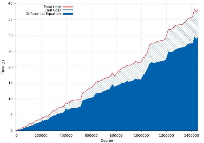
Timings obtained with magma v2.24-10 on a laptop with an intel processor i7-8850h@2.60ghz

Figure 1. Isogeny computations in $\mathbb{F}_{2}$.

3. Applications

Thanks to the results of [BMSS08, LS08, LV16] in odd characteristic and the case of characteristic 2 being solved in Section 2, we now have in all characteristic fast algorithms for computing isogenies, at least if we have a Weierstrass model of the isogenous curve and the isogeny differential. In this section, we are interested in the calculation of irreducible polynomials. We show how we can extend to the case of very small finite fields, especially $\mathbb{F}_{2}$, the construction of [CL13]. With this aim, we start with a brief presentation on endomorphism rings and isogenies in Section 3.1, and show in Section 3.2 how to calculate the isogenous curves and the isogeny differentials over finite fields of small characteristic. Then, in Section 3.3, we apply this construction to build irreducible polynomials and we end with an example in Section 3.4.

3.1. Endomorphism ring and isogenies

We briefly introduce some facts about the theory of complex multiplication. Good references are [Lan73, Sil94, Cox13].

An isogeny $E_{1}\rightarrow E_{2}$ of elliptic curves defined over a field $k$ is a surjective morphism of curves that induces a group homomorphism $E_{1}(\bar{k})\rightarrow E_{2}(\bar{k})$. We denote by $\operatorname{Hom}_{k}(E_{1},E_{2})$ the set of homomorphisms from $E_{1}$ to $E_{2}$ over $k$ and let $\operatorname{End}_{k}(E)=\operatorname{Hom}_{k}(E,E)$. We write $\operatorname{End}(E)=\operatorname{End}_{\bar{k}}(E)$. Composition of endomorphisms gives a ring structure on $\mathcal{O}=\operatorname{End}(E)$, and we refer to $\mathcal{O}$ as the ring of endomorphisms of $E$.

As a $\mathbb{Z}$-module, $\operatorname{End}_{k}(E)$ is free of rank at most four. More precisely, $\operatorname{End}_{k}(E)$ is either $\mathbb{Z}$, an order in an imaginary quadratic field (ordinary case) or an order in a definite quaternion algebra (supersingular case). By definition, ordinary or supersingular elliptic curves have complex multiplication. Moreover, every endomorphism $\varphi$ satisfies in $\operatorname{End}_{k}(E)$ a quadratic characteristic polynomial with integer coefficients, $\varphi^{2}-t\,\varphi+d=0\,.$ The integer $t$, denoted $\operatorname{Tr}(\varphi)$, is called the trace of $\varphi$. Over $k=\mathbb{F}_{q}$, the Frobenius endomorphism $\phi_{q}$ takes a leading role, since it determines the group and $\operatorname{End}_{k}(E)$-structure of the rational points of $E$ [Len96]. In particular, it satisfies the Weil polynomial

$$\phi_{q}^{2}-t\,\phi_{q}+q=0$$ (22)

where $t=\operatorname{Tr}\phi_{q}=:\operatorname{Tr}E$ is such that $q+1-t$ is the number of rational points of $E$ over $k$.

What follows is for elliptic curves over $\mathbb{C}$, but these results reduce well to elliptic curves over finite fields. In the ordinary case, let $\mathcal{O}$ be an order in an imaginary quadratic field $\kappa$. Then the theory of complex multiplication states that there is a number field $L$ containing $\kappa$ and an elliptic curve $E$ over $L$ with $\operatorname{End}_{\bar{L}}(E)=\mathcal{O}$. Let $p$ be a prime that splits completely in $\mathcal{O}_{L}$ and $\mathfrak{p}$ be a prime of $\mathcal{O}_{L}$ above $p$, so that $\mathcal{O}_{L}/{\mathfrak{p}}\simeq\mathbb{F}_{p}$. If $\mathfrak{p}$ does not divide the discriminant of $E$, then $E$ has good reduction modulo $\mathfrak{p}$. Let $\bar{E}$ denote this reduction, then $\operatorname{End}_{\bar{\mathbb{F}}_{p}}(\bar{E})\simeq\mathcal{O}$. Conversely, every elliptic curve $\bar{E}$ arises as the reduction of an elliptic curve $E$ over some $L$ with same ring of endomorphisms $\mathcal{O}$, called the canonical lift of $\bar{E}$.

There is a one-to-one correspondence between the isomorphism classes of elliptic curves $E/\mathbb{F}_{q}$ with $\operatorname{End}(E)=\mathcal{O}$ and the ideal class group $\operatorname{Cl}(\mathcal{O})$ (i.e. the quotient group of the fractional $\mathcal{O}$-ideals that are prime to the conductor $\mathcal{O}$ by its subgroup of principal ideals). To an invertible $\mathcal{O}$-ideal $\mathfrak{a}$, one associates the elliptic curve $E_{\mathfrak{a}}\simeq\mathbb{C}/\mathfrak{a}$. An ideal $\mathfrak{a}^{\prime}$ is equivalent to $\mathfrak{a}$ in $\operatorname{Cl}(\mathcal{O})$ if and only if $\mathbb{C}/\mathfrak{a}^{\prime}$ is isomorphic to $E_{\mathfrak{a}}$.

Let now $\mathfrak{l}$ be an invertible $\mathcal{O}$-ideal, and define the the kernel of $\mathfrak{l}$ in $E_{\mathfrak{a}}$ to be the intersection of the kernels of all endomorphisms in $\mathfrak{l}$. We denote it $E_{\mathfrak{a}}[\mathfrak{l}]$,

$$E_{\mathfrak{a}}[\mathfrak{l}] \simeq \{z\in\mathbb{C}:\alpha z\in\mathfrak{a},\ \text{for all}\ \alpha\in\mathfrak{l}\subset\operatorname{End}(E_{\mathfrak{a}})\}\,,$$

$$\simeq \mathfrak{l}^{-1}\mathfrak{a}/\mathfrak{a}.$$

The identity map on $\mathbb{C}$ induces the isogeny $I:\mathbb{C}/\mathfrak{a}\rightarrow\mathbb{C}/\mathfrak{l}^{-1}\mathfrak{a}$ with kernel $E_{\mathfrak{a}}[\mathfrak{l}]$. The norm of $\mathfrak{l}$ is equal to the degree of the isogeny. The terminology “quotient isogeny” is sometimes used, together with the notation $I:E_{\mathfrak{a}}\rightarrow E_{\mathfrak{a}}/E_{\mathfrak{a}}[\mathfrak{l}]$.

Every isogeny between elliptic curves with isomorphic ring of endomorphisms arises in this way. In particular, let $I_{1}:E_{1}\rightarrow E_{2}$ be a first isogeny defined by $\mathfrak{l_{1}}$, and $I_{2}:E_{2}\rightarrow E_{3}$ be a second isogeny defined by $\mathfrak{l_{2}}$, then the kernel of $I_{2}\circ I_{1}:\lx@xy@svg{\hbox{\raise 0.0pt\hbox{\kern 8.37915pt\hbox{\ignorespaces\ignorespaces\ignorespaces\hbox{\vtop{\kern 0.0pt\offinterlineskip\halign{\entry@#!@&&\entry@@#!@\cr&&\crcr}}}\ignorespaces{\hbox{\kern-8.37915pt\raise 0.0pt\hbox{\hbox{\kern 0.0pt\raise 0.0pt\hbox{\hbox{\kern 3.0pt\raise 0.0pt\hbox{$\textstyle{E_{1}\ignorespaces\ignorespaces\ignorespaces\ignorespaces}$}}}}}}}\ignorespaces\ignorespaces\ignorespaces\ignorespaces{}{\hbox{\lx@xy@droprule}}\ignorespaces\ignorespaces\ignorespaces{\hbox{\kern 14.56596pt\raise 6.0361pt\hbox{{}\hbox{\kern 0.0pt\raise 0.0pt\hbox{\hbox{\kern 3.0pt\hbox{\hbox{\kern 0.0pt\raise-1.74722pt\hbox{$\scriptstyle{I_{1}}$}}}\kern 3.0pt}}}}}}\ignorespaces{\hbox{\kern 32.37915pt\raise 0.0pt\hbox{\hbox{\kern 0.0pt\raise 0.0pt\hbox{\lx@xy@tip{1}\lx@xy@tip{-1}}}}}}{\hbox{\lx@xy@droprule}}{\hbox{\lx@xy@droprule}}{\hbox{\kern 32.37915pt\raise 0.0pt\hbox{\hbox{\kern 0.0pt\raise 0.0pt\hbox{\hbox{\kern 3.0pt\raise 0.0pt\hbox{$\textstyle{E_{2}\ignorespaces\ignorespaces\ignorespaces\ignorespaces}$}}}}}}}\ignorespaces\ignorespaces\ignorespaces\ignorespaces{}{\hbox{\lx@xy@droprule}}\ignorespaces\ignorespaces\ignorespaces{\hbox{\kern 55.32426pt\raise 6.0361pt\hbox{{}\hbox{\kern 0.0pt\raise 0.0pt\hbox{\hbox{\kern 3.0pt\hbox{\hbox{\kern 0.0pt\raise-1.74722pt\hbox{$\scriptstyle{I_{2}}$}}}\kern 3.0pt}}}}}}\ignorespaces{\hbox{\kern 73.13745pt\raise 0.0pt\hbox{\hbox{\kern 0.0pt\raise 0.0pt\hbox{\lx@xy@tip{1}\lx@xy@tip{-1}}}}}}{\hbox{\lx@xy@droprule}}{\hbox{\lx@xy@droprule}}{\hbox{\kern 73.13745pt\raise 0.0pt\hbox{\hbox{\kern 0.0pt\raise 0.0pt\hbox{\hbox{\kern 3.0pt\raise 0.0pt\hbox{$\textstyle{E_{3}}$}}}}}}}\ignorespaces}}}}\ignorespaces$ is $E_{1}[\mathfrak{l}_{1}\mathfrak{l}_{2}]$.

These facts are well summarized in the following proposition.

Proposition 20 ([Sil94, Prop. 1.2, Chap. II]).

1. Let $E_{\mathfrak{a}}$ be an elliptic curve with endomorphism ring ${\mathcal{O}}_{\kappa}$ and let $\mathfrak{l}$ and $\mathfrak{l}^{\prime}$ be non-zero fractional ideals of ${\mathcal{O}}_{\kappa}$.

   1. $\mathfrak{l}\,\mathfrak{a}$ is a lattice in $\mathbb{C}$.

   2. The elliptic curve $E_{\,\mathfrak{l}\,\mathfrak{a}}$ satisfies $\operatorname{End}(E_{\,\mathfrak{l}\,\mathfrak{a}})\simeq{\mathcal{O}}_{\kappa}$.

   3. $E_{\,\mathfrak{l}\,\mathfrak{a}}\simeq E_{\,\mathfrak{l}^{\prime}\,\mathfrak{a}}$ if and only if $\mathfrak{l}\simeq\mathfrak{l}^{\prime}$ in $\operatorname{Cl}(\mathcal{O_{\kappa}})$.

   Hence there is a well-defined action of $\operatorname{Cl}(\mathcal{O_{\kappa}})$ on the set of elliptic curves with endomorphism ring ${\mathcal{O}}_{\kappa}$ determined by $\mathfrak{l}*E_{\mathfrak{a}}=E_{\,\mathfrak{l}^{-1}\,\mathfrak{a}}\,.$

2. The action of $\operatorname{Cl}(\mathcal{O_{\kappa}})$ described in (a) is simply transitive. In particular $\#\operatorname{Cl}(\mathcal{O_{\kappa}})$ is equal to the number of elliptic curves with endomorphism ring ${\mathcal{O}}_{\kappa}$.

3.2. Isogenies of large degree

Let $E$ be an elliptic curve with complex multiplication defined over a finite field $k$ and $\ell>2$ a large prime integer. Here, the field of definition of $E$ is supposed to be very small compared to $\ell$ so that in this case, up to an endomorphism, an $\ell$-isogeny can be written as a composition of small isogenies. This can be done by working in the ideal class group of the endomorphism ring of $E$. In fact, the situation is very similar to that behind the algorithm given by Kohel in his thesis for computing the endomorphism ring of an elliptic curve.

Theorem 21 ([Koh96, Th. 1]).

There exists a deterministic algorithm that, given an elliptic curve $E$ over a finite field $k$ of $q$ elements, computes the isomorphism type of the endomorphism ring of $E$ and if a certain generalization of the Riemann hypothesis holds true, for any $\varepsilon>0$ runs in time $O(q^{1/3+\varepsilon})$.

Since in our case of interest, the field of definition of the curves is rather small while the degrees of the isogenies are rather large, we can suppose that we are given the endomorphism ring $\operatorname{End}(E)$ of $E$ as an order $\mathcal{O}_{\kappa}$ in an imaginary quadratic field $\kappa=\mathbb{Q}(\sqrt{-\Delta})$, $\Delta$ a primitive discriminant. For the sake of simplicity, we assume that this order is maximal, i.e. equal to the ring of integers $\mathbb{Z}[\omega]$ of $\kappa$.

In this context, a prime integer $\ell\neq p$ that splits in $\kappa$ is usually called an Elkies prime for $E$. We more generally define Elkies degrees for $E$ as integers whose prime divisors are all Elkies primes for $E$. Incidentally, there exist a $k$-rational $\ell$-isogeny from $E/k$ to another curve $\tilde{E}/k$. This said, the computation of the isogenous curve $\tilde{E}$ reduces to calculations in the ideal class group of $\mathcal{O}_{\kappa}$.

More precisely, let $m$ be one of the Elkies prime divisors of $\ell$. Let $\operatorname{Cl}(\mathcal{O}_{\kappa})$ be the ideal class group associated to $\mathcal{O}_{\kappa}$ . We have $|\text{Cl}(\mathcal{O}_{\kappa})|=O(\sqrt{|\Delta|})\,.$ In addition, every ideal class in $\operatorname{Cl}(\mathcal{O}_{\kappa})$ contains an ideal of norm less than $\sqrt{|\Delta|}$. So, $\operatorname{Cl}(\mathcal{O}_{\kappa})$ is generated by classes of ideals of norm less than $\sqrt{|\Delta|}$. Let $\mathfrak{m}$ be an ideal $(m,a_{\mathfrak{m}}+b_{\mathfrak{m}}\,\omega)$ in $\mathcal{O}_{\kappa}$ that divides $(m)$, and write $\mathfrak{u}_{1}\>\mathfrak{m}=\mathfrak{u}_{2}\>\prod\limits_{i=1}^{h}{\mathfrak{p}_{i}^{e_{i}}}\,,$ where $\operatorname{Norm}(\mathfrak{p}_{i})\leq\sqrt{\Delta}$ and $\mathfrak{u}_{1}$ and $\mathfrak{u}_{2}$ are two principal ideals. Each prime ideal $\mathfrak{p}_{i}$ determines an isogeny, and $\mathfrak{u}_{1}$, $\mathfrak{u}_{2}$ correspond to endomorphisms. Their product yields the isogeny defined by the following chain of small degree isogenies,

$$E\longrightarrow{\raisebox{1.99997pt}{$E$}\left/\raisebox{-1.99997pt}{$E[\mathfrak{p}_{1}]$}\right.}\longrightarrow{\raisebox{1.99997pt}{$E$}\left/\raisebox{-1.99997pt}{$E[\mathfrak{p}_{1}^{2}]$}\right.}\longrightarrow\ldots\longrightarrow{\raisebox{1.99997pt}{$E$}\left/\raisebox{-1.99997pt}{$E[\mathfrak{p}_{1}^{e_{1}}]$}\right.}\longrightarrow\\ {\raisebox{1.99997pt}{$E$}\left/\raisebox{-1.99997pt}{$E[\mathfrak{p}_{1}^{e_{1}}\mathfrak{p}_{2}]$}\right.}\longrightarrow{\raisebox{1.99997pt}{$E$}\left/\raisebox{-1.99997pt}{$E[\mathfrak{p}_{1}^{e_{1}}\mathfrak{p}_{2}^{2}]$}\right.}\longrightarrow\ldots\longrightarrow{\raisebox{1.99997pt}{$E$}\left/\raisebox{-1.99997pt}{$E[\mathfrak{p}_{1}^{e_{1}}\mathfrak{p}_{2}^{e_{2}}]$}\right.}\longrightarrow\\ \ldots\\ {\raisebox{1.99997pt}{$E$}\left/\raisebox{-1.99997pt}{$E[\mathfrak{p}_{1}^{e_{1}}\mathfrak{p}_{2}^{e_{2}}\cdots\mathfrak{p}_{h-1}^{e_{h-1}}\mathfrak{p}_{h}]$}\right.}\longrightarrow\cdots\longrightarrow{\raisebox{1.99997pt}{$E$}\left/\raisebox{-1.99997pt}{$E[\mathfrak{p}_{1}^{e_{1}}\mathfrak{p}_{2}^{e_{2}}\cdots\mathfrak{p}_{h}^{e_{h}}]$}\right.}\,.$$ (23)

We arrive in this way at the isogenous curve $\tilde{E}={E}\,/\,{E[\mathfrak{p}_{1}^{e_{1}}\,\mathfrak{p}_{2}^{e_{2}}\,\cdots\,\mathfrak{p}_{h}^{e_{h}}]}$.

To avoid the divisions by $p$ that do appear in calculations for computing explicitly all these isogenies, we reconsider Chain (23) from the standpoint of the canonical lifts of these curves. Results by Serre and Tate [LST64] enable to lift canonically $E$ as $\mathcal{E}/K$ where $K$ is an unramified extension of $\mathbb{Q}_{p}$ of degree $n$ such that $k$ is its residue field.

An algorithm for computing canonical lifts at $p$-adic precision $N$ in time complexity $O(p^{2}\,N^{2})$ up to some polylogarithmic factors can be for instance found in [Sat00, SST03]. According to Theorem 11 and [LV16, Theorem 2], the lifting process has to be done with $p$-adic precision equal to $O(\lceil\log_{p}(\ell)\rceil)$ in order to be able to reduce the results modulo $p$. Since in this situation the principal ideal $(q)$ splits in $\mathcal{O}_{\kappa}$ into two prime ideals, one chooses arbitrarily the residue field given by one of the two, which allows us to embed integers from $O_{\kappa}$ into $K$, $\omega\mapsto\sqrt{-\Delta}$.

Now, starting from $\mathcal{E}$ in Chain (23), we use Vélu’s formulas to compute for each $\mathfrak{p}_{i}$ a normalized isogenous curve [Vél71]. These formulas require that one knows the kernels $\mathcal{E}[\mathfrak{p}_{i}]$. This can be easily done for small degrees, e.g. degree 2, by factoring division polynomials. When this approach (of cubic complexity in the degree) is too expansive, an alternative approach is to use modular polynomials. It enables to find the $j$-invariant of the isogenous curve. Motivated by point counting on elliptic curves, Elkies gave an elegant method to derive from it an explicit normalized equation for this isogenous curve. This algorithm, of quadratic complexity in the degree, is far beyond the scope of this paper and we refer to [Sch95] for details. This process yields a $\prod_{i=1}^{h}\mathfrak{p}_{i}^{e_{i}}$-isogenous curve $\tilde{\mathcal{E}}$. Furthermore, the curve $\tilde{\mathcal{E}}$ is also $m$-isogenous to $\mathcal{E}$ up to the endomorphism $\mathfrak{u}_{2}\mathfrak{u}_{1}^{-1}$. The differential of this $m$-isogeny is thus equal to the embedding of $\mathfrak{u}_{2}\,\mathfrak{u}_{1}^{-1}$ in $K$ .

We now iterate this construction for every remaining prime divisor $m$ of $\ell$, counting multiplicity, and go from one isogenous curve to the next. We arrive in this way to a $\ell$-isogenous curve, and its differential. Recall that it is faster to compute the isogeny from $\mathcal{E}$ to $\tilde{\mathcal{E}}$ than computing all the $\mathfrak{p}_{i}$-isogenies and composing them (see Remark 14). We call Algorithm 2 to find the solution $z(t)$ of Eq. (7) modulo $t^{2\ell+2}$. It remains to reduce $z(t)$ modulo $p$ and compute its Padé approximant to recover the rational function that gives the isogeny.

The conclusion of this section is that we can compute an $\ell$-isogenous curve and a rational representation of the isogeny in quasi-linear time in $\ell$ when $\ell\gg q$.

Theorem 22.

Given an ordinary elliptic curve $E$ defined over a finite field $k$ with characteristic $p$ and cardinality $q=p^{n}$ such that its endomorphism ring $\mathcal{O}_{\kappa}$ is maximal and $\ell$ is an Elkies degree for $E$, there exists an algorithm that computes an equation of an $\ell$-isogenous curve $\tilde{E}$ of $E$ and the isogeny with time complexity $O(n\,\ell+p^{2}+q^{3/2})$ up to some polylogarithmic factors.

Under reasonable heuristic assumptions detailed in [BS11], the $q^{3/2}$ term can be replaced by $L\left[1/2,\sqrt{3}/2\right](q)$ where $L$ denotes the usual subexponential functions

$$L\left[\alpha,{\mathsf{c}}\right]\left(x\right)=\exp(\,\left({\mathsf{c}}+o(1)\right)\,\left(\log x\right)^{\alpha}\,\left(\log\log x\right)^{1-\alpha}\,)\,.$$

Remark 23.

In some cases, the isogeny differential $c$ is rational and the lifting does not need to be canonical. For example if $\ell$ is an integer coprime to $p$, then the multiplication map $[\ell]\>:E\longrightarrow E$ is a separable isogeny that can be computed by lifting arbitrarily the equation of the curve $E$ and taking $c=1/{\ell}$ in $\mathbb{Q}_{q}$.

3.3. Irreducible polynomials over finite fields

Given a finite field $k$, with characteristic $p$ and cardinality $q=p^{n}$, and a degree $d$, the Couveignes-Lercier Las Vegas algorithm achieves a notable quasi-linear asymptotic complexity in $d$ for computing an irreducible polynomial of degree $d$ over $k$ [CL13]. It is based on elliptic curves with a number of points which is divisible by prime divisors of $d$. So, these curves define separable isogenies whose kernels have only rational points. In its primary form (see Lemma 24), this algorithm yields a highly efficient method to calculate an irreducible polynomial when $d$ is a prime not dividing $p\,(q-1)$ such that $4d\leqslant{q^{\frac{1}{4}}}{}$. For the sake of completeness, we briefly present this construction in Section 3.3.1.

However, we note that when $d$ is not a prime or when $d$ is larger than $q+1+2\,\sqrt{q}$, [CL13] necessarily involves the use of the Kedlaya-Umans algorithm [KU11]. Unfortunately, this algorithm is widely considered impractical, and in our case of interest where $q$ is negligible compared to $d$, especially the important case $k=\mathbb{F}_{2}$, we can no more rely on this method.

We show in this section that we can adapt the construction to elliptic curves that do not necessarily have a cardinality divisible by the prime divisors of $d$. They simply have to admit rational isogenies of degree $\ell$ where $\ell$ is of the form $p_{1}^{e_{1}}$ or of the form $p_{1}^{e_{1}}\,p_{2}^{e_{2}}$ with $p_{1}$ and $p_{2}$ odd prime integers. Given an elliptic curve, it yields an infinite dense list of reachable degrees $d$. Except for the few degrees $d$ that can not be written as $d=\phi(\ell)$ or $d=\phi(\ell)/2$, we more generally have good expectation to find an elliptic curve that may work for a degree $d$ fixed in advance. We develop this aspect in Section 3.3.2.

3.3.1. Overview of [CL13]

Let $I/k:E/k\rightarrow\tilde{E}/k$ be a degree $\ell$ separable isogeny where $E/k$ and $\tilde{E}/k$ is given by an affine Weierstrass equation in $x$, $y$. We denote by $O_{E}$ and $O_{\tilde{E}}$ the points at infinity of $E$ and $\tilde{E}$.

We assume that $\ell$ is a positive odd number and the kernel $\mathop{\rm{Ker}}\nolimits I$ is cyclic. Let $T\in E({\bar{k}})$ be a generator of $\mathop{\rm{Ker}}\nolimits I$. Let $\psi_{I}(x)\in k[x]$ be the degree $(\ell-1)/2$ polynomial

$$\psi_{I}(x)=\prod_{1\leqslant k\leqslant(\ell-1)/2}(x-x(kT))\,.$$ (24)

There exists a degree $\ell$ polynomial $\phi_{I}(x)\in k[x]$ such that the image of the abscissa of the point $(x,y)$ by $I$ is $\eta(x)={\phi_{I}(x)}/{\psi_{I}^{2}(x)}$.

Now, let $A$ be a $k$-rational point on $\tilde{E}$ such that $2A\not=O_{\tilde{E}}$ and let $B\in E({\bar{k}})$ be a point on $E$ such that $I(B)=A$. We can define the degree $\ell$ polynomial

$$f_{I,A}(x)=\phi_{I}(x)-x(A)\psi_{I}^{2}(x)\in k[x].$$

Its roots are the $x(B+kT)$ for $0\leqslant k<d$, and they are pairwise distinct because $2A\not=O_{\tilde{E}}$. So $f_{I,A}(x)$ is a degree $\ell$ separable polynomial. Furthermore, it is reducible if and only if the fiber $I^{-1}(A)$ is.

This happens to be true when $A$ is a point of order $\ell$, and $\ell$ is a prime not dividing $p\,(q-1)$ such that it divides exactly the number $q+1-\operatorname{Tr}E$ of rational points of $E$. In this case, the Weil polynomial (22) splits as $(X-r)\,(X-s)\bmod\ell$ such that $r=1\bmod\ell$ and $s=q\bmod\ell$. Especially the Galois orbit of $B$ has cardinality $\ell$ since $\phi_{q}(B)=r\,B$ and the order of $r$ is $\ell$ in $(\mathbb{Z}/\ell^{2}\mathbb{Z})^{\times}$ [CL13, Section 4.2].

When $\ell$ is small enough, we can find with high confidence such an elliptic curve $E$. All in all, it yields a quite efficient method to compute an irreducible polynomial.

Lemma 24 ([CL13, Lemma 6 ($\delta=1$)]).

There exists a probabilistic (Las Vegas) algorithm that on input a finite field $k$ with characteristic $p$ and cardinality $q=p^{n}$, a prime integer $\ell$ not dividing $p\,(q-1)$ such that $4\ell\leqslant{q^{\frac{1}{4}}}{}$, computes an irreducible polynomial in $k[x]$ of degree $\ell$, at the expense of $\ell\times(\log q)^{5+o(q)}+\ell^{1+o(\ell)}\times(\log q)^{1+o(q)}$ elementary operations.

3.3.2. An extended algorithm

Let now $\ell$ be an odd Elkies degree, prime to $p\,(q-1)$. The integer $\ell$ is thus odd. More specifically, it will become clear later on that $\ell$ is the product of at most two prime powers. With the notations of Section 3.2, we denote by $\sigma_{q}$ the image of the Frobenius endomorphism $\phi_{q}$ in $\mathcal{O}_{\kappa}$. In this setting, let $\mathfrak{l}$ be an ideal in $\mathcal{O}_{\kappa}$ above $\ell$ and containing $\sigma_{q}-r$ where $r\in\mathbb{Z}/{\ell}\mathbb{Z}$ is a root of $X^{2}-\operatorname{Tr}(E)\,X+q\bmod\ell$.

Take for $A$ the point at infinity $O_{\tilde{E}}$ in the construction of Section 3.3.1. We thus consider the polynomial $f_{I,O_{\tilde{E}}}(x)=\psi(x)$, whose roots are the abscissas of points in $\mathop{\rm{Ker}}\nolimits I$. Now, the factorizations $I=I_{\ell/m}\circ I_{m}$, where $I_{m}$ are isogenies of degree $m$ with $m$ any divisor of $\ell$, yield $\mathop{\rm{Ker}}\nolimits I_{m}\subset\mathop{\rm{Ker}}\nolimits I$. Consequently, the polynomial $\psi(x)$ splits as

$$\psi(x)=\prod\limits_{m\,|\,\ell}\Psi_{m}(x)\,,$$

with $\deg\Psi_{m}(x)=\varphi(m)/2$, the Euler’s totient function of $m$. Computing $I_{m}$ for $m\neq\ell$ by the same procedure as $I$, we can obtain $\Psi_{m}(x)$. Dividing $\psi(x)$ by all of them, we are led to examine the polynomial $\Psi_{\ell}(x)$, of degree $\varphi(\ell)/2$. Here too, its irreducibility depends on the order of $r$ in the multiplicative group $(\mathbb{Z}/{\ell}\mathbb{Z})^{\times}$ because the length of the Galois orbit of $B$ is determined by the relation $\phi_{q}(B)=r\,B$. The polynomial $\Psi_{\ell}(x)$ splits thus in factors of degree $d=\operatorname{ord}_{\mathbb{Z}/{\ell}\mathbb{Z}}(r)/2$ or $d=\operatorname{ord}_{\mathbb{Z}/{\ell}\mathbb{Z}}(r)$ according to whether a power of $r$ is equal to $-1$ or not. When $d=\varphi(\ell)/2$, the polynomial $\Psi_{\ell}(x)$ is therefore irreducible.

For the same reasons, take for $B$ any non-zero point of ${E}(k)$ and take $A=I(B)$, then the polynomial

$$\nu_{I,A}(x)=f_{I,A}(x)\,/\,(\,x-x(B)\,)\,,$$

of degree $\ell-1$, splits in factors $\Phi_{m}(x)$ of degree $\varphi(m)$ where $m\neq 1$ divides $\ell$ . In turn, $\Phi_{\ell}(x)$ splits in factors of degree $\operatorname{ord}_{\mathbb{Z}/{\ell}\mathbb{Z}}(r)$ . The polynomial $\Phi_{\ell}(x)$ is thus irreducible when $\operatorname{ord}_{\mathbb{Z}/{\ell}\mathbb{Z}}(r)=\varphi(\ell)$.

The main part of this construction is thus to determine the isogenous curve $\tilde{E}$ and the equations of the isogeny $I$ following Theorem 22. Therefore, we can state this theorem.

Theorem 25.

Given an ordinary elliptic curve $E$ defined over a finite field $k$ with characteristic $p$ and cardinality $q=p^{n}$, and $\ell$, product of at most two prime powers, an odd Elkies degree prime to $p\,(q-1)$ such that one of the roots $r$ modulo $\ell$ of the Weil polynomial $X^{2}-(\operatorname{Tr}E)\,X+q$ has order $\varphi(\ell)$ in $(\mathbb{Z}/\ell\mathbb{Z})^{\times}$, there exists an algorithm that computes two irreducible polynomials in $k$ of degree $\varphi(\ell)$ and $\varphi(\ell)/2$ with time complexity $O(n\,\ell+p^{2}+q^{3/2})$ up to some polylogarithmic factors.

With same complexity, this algorithm computes an irreducible polynomial of degree $\varphi(\ell)/2$ when $\operatorname{ord}_{\mathbb{Z}/{\ell}\mathbb{Z}}(r)=\varphi(\ell)/2$ and $-1\notin\langle r\rangle$ .

Note that, since $\ell$ is odd and $\operatorname{ord}_{\mathbb{Z}/{\ell}\mathbb{Z}}(r)$ can not be larger than the Carmichael function $\lambda(\ell)$, we have that $\ell$ is either of the form $p_{1}^{e_{1}}$ or of the form $p_{1}^{e_{1}}\,p_{2}^{e_{2}}$ where $p_{1}$ and $p_{2}$ are odd prime integers. The former corresponds to the only possibility for $(\mathbb{Z}/{\ell}\mathbb{Z})^{\times}$ to be cyclic (e.g. $\lambda(\ell)=\varphi(\ell)$ and $\operatorname{ord}_{\mathbb{Z}/{\ell}\mathbb{Z}}(r)=\lambda(\ell)/2$), the latter (e.g. $\operatorname{ord}_{\mathbb{Z}/{\ell}\mathbb{Z}}(r)=\lambda(\ell)=\varphi(\ell)/2$ ) follows from the recursive definition of $\lambda$,

$$\lambda(p_{1}^{e_{1}}\cdot p_{2}^{e_{2}}\cdots p_{k}^{e_{k}})=\operatorname{lcm}\left(\lambda(p_{1}^{e_{1}}),\lambda(p_{2}^{e_{2}}),\ldots,\lambda(p_{k}^{e_{k}})\right)\,.$$

Also note that $\varphi(\ell)$ is nearly $\ell$ in Theorem 25, since the necessary conditions on $\ell$ yields $\varphi(\ell)=p_{1}^{e_{1}-1}(p_{1}-1)$ or $\varphi(\ell)=p_{1}^{e_{1}-1}(p_{1}-1)\,p_{2}^{e_{2}-1}(p_{2}-1)$.

Remark 26.

Applied to the elliptic curve $E\,/\,\mathbb{F}_{2}:y^{2}+x\,y=x^{3}+1\,$, whose Weil polynomial is $X^{2}+X+2$, this method gives an infinite list of irreducible polynomials over $\mathbb{F}_{2}$, of degree

$$3,\ 5,\ 6,\ 10,\ 11,\ 14,\ 21,\ 26,\ 28,\ 30,\ 33,\ 35,\ 39,\ 42,\ 52,\ 53,\ 54,\ 55,\ 56,\ 63,\ 66,\ \\ 70,\ 74,\ 75,\ 78,\ 81,\ 84,\ 89,\ 95,\ 96,\ 98,105,106,108,110,112,119,131,138\ldots$$

We give for the first ones the degree $\ell$ of the isogeny, the root $r$ of $X^{2}+X+2$ and its order modulo $\ell$ in the following table.

$d$	3	5	5	6	10	11	14	21	21	26	28	30	33	33	35	39	42	52
$\ell$	7	11	11	7	11	23	29	43	43	53	29	77	67	67	71	79	43	53
$r$	3	6	4	3	6	13	21	24	18	14	21	59	55	11	31	66	18	14
$\operatorname{ord}_{\ell}(r)$	6	10	5	6	10	11	28	21	42	52	28	30	33	66	70	78	42	52

Remark 27.

Similarly to Remark 26, we can easily do an exhaustive search on degrees that are not reachable with this method, whatever the field or the curve are. The first ones are

$$7,\ 13,\ 17,\ 19,\ 24,\ 25,\ 31,\ 32,\ 34,\ 37,\ 38,\ 43,\ 45,\ 47,\ 49,\ 57,\ 59,\ 61,\ 62,\ 64,\\ 67,\ 71,\ 73,\ 76,\ 77,\ 79,\ 85,\ 87,\ 91,\ 93,\ 94,\ 97,\ 101,\ 103,\ 104,\ 107,\ 109\ldots$$

For instance, degree $7$ is not possible because there is no integer $\ell$ such that $\varphi(\ell)$ equals $7$ or $14$.

Remark 28.

Theorem 22 and Theorem 25 can be extended to supersingular elliptic curves if we lift them together with a quadratic order (see for instance [CH02]).

3.4. An example

We consider the finite field $\mathbb{F}_{16}=\mathbb{F}_{2}(v)$ such that $v^{4}+v+1=0$. Let $E$ be the elliptic curve defined by $E/\mathbb{F}_{16}\>:y^{2}+xy=x^{3}+v^{6}$. Choose $\ell=73$, the Weil polynomial of $E$ satisfies

$$X^{2}+3X+16\equiv(X-10)\,(X-60)\>\bmod\ell\,.$$

The endomorphism ring of $E$ is isomorphic to the ring of integers $\mathcal{O}$ of the quadratic field $\mathbb{Q}(\sqrt{-55})$. The class group $\operatorname{Cl}(\mathcal{O})$ is cyclic of order 4. Let $\mathfrak{l}$ be the ideal of $\mathcal{O}$ generated by $73$ and $\phi_{16}-60$. The set $E[\mathfrak{l}]$ is a cyclic subgroup of $E$ of order $73$, closed under the action of the Frobenius endomorphism. Let $I\>:E\longrightarrow{E}/{E[\mathfrak{l}]}$ be the degree $73$ isogeny with kernel $E[\mathfrak{l}]$. We give the first coordinate of $I$ as the rational fraction ${\phi(x)}/{\psi(x)^{2}}$. Note that $\psi$ is a degree $36$ irreducible polynomial since $60$ is a generator of the multiplicative group $\mathbb{F}_{73}^{\times}$.

Let us compute $\psi(x)$. The ideal $\mathfrak{l}$ can be decomposed as $\mathfrak{p}\,\mathfrak{l}=\mathfrak{u}_{2}\,,$ where $\mathfrak{p}=(2,(\sqrt{-55}+1)/2)$ and $\mathfrak{u}_{2}=(-\sqrt{-55}+23)/2$. We begin by lifting $E$ in the $2$-adics such that $\operatorname{End}(E)=$ $\operatorname{End}(\mathcal{E})$ as

$$\mathcal{E}:y^{2}+xy=x^{3}+21\,v^{3}+261\,v^{2}+316\,v+256+O(2^{10})\,.$$

In order to compute an equation of $\tilde{\mathcal{E}}$ and the differential isogeny, we first construct the degree $2$ isogeny ${\mathcal{E}}\,/\,{\mathcal{E}[\mathfrak{p}]}\cong\tilde{\mathcal{E}}\longrightarrow\mathcal{E}\,,$ we deduce

$${\mathcal{E}}\,/\,{\mathcal{E}[\mathfrak{p}]}:y^{2}=x^{3}-(27+O(2^{10}))x+2(-224\,v^{3}+96\,v^{2}-160,v+315)+O(2^{11}).$$

In return, a $73$-isogenous curve $\tilde{E}$ to $E$ is given by

$$\tilde{E}\>:y^{2}+xy=x^{3}+v^{12}\,$$

and the isogeny differential is

$$c=244v^{3}+164v^{2}-424v-299+O(2^{10})\,.$$

Applying Algorithm 2 with $U(t)=4(21v^{3}+261v^{2}+316v+256+O(2^{10}))\,t^{4}+t+4$ and $V(t)=4(v^{3}+123v^{2}+243v+369+O(2^{10})))\,t^{4}+t+4$ and $c$, and reducing modulo $2$ we get the series $z(t)$. A final call to the half-gcd algorithm yields the irreducible polynomial

$$\psi(x)=\overline{\mathtt{F}}+\overline{\mathtt{E}}\,x+\overline{\mathtt{7}}\,x^{2}+\overline{\mathtt{B}}\,x^{3}+\overline{\mathtt{7}}\,x^{4}+\overline{\mathtt{B}}\,x^{5}+\overline{\mathtt{E}}\,x^{6}+\overline{\mathtt{7}}\,x^{7}+\overline{\mathtt{2}}\,x^{9}+\overline{\mathtt{B}}\,x^{10}+\overline{\mathtt{7}}\,x^{13}\\ +\overline{\mathtt{9}}\,x^{14}+\overline{\mathtt{E}}\,x^{15}+\overline{\mathtt{7}}\,x^{16}+\overline{\mathtt{F}}\,x^{17}+\overline{\mathtt{6}}\,x^{18}+\overline{\mathtt{5}}\,x^{19}+\overline{\mathtt{D}}\,x^{20}+\overline{\mathtt{6}}\,x^{21}+\overline{\mathtt{1}}\,x^{22}+\overline{\mathtt{C}}\,x^{23}+\overline{\mathtt{7}}\,x^{24}\\ +\overline{\mathtt{B}}\,x^{26}+\overline{\mathtt{2}}\,x^{27}+\overline{\mathtt{3}}\,x^{28}+\overline{\mathtt{2}}\,x^{29}+\overline{\mathtt{5}}\,x^{30}+\overline{\mathtt{A}}\,x^{31}+\overline{\mathtt{C}}\,x^{32}+\overline{\mathtt{7}}\,x^{33}+\overline{\mathtt{9}}\,x^{34}+\overline{\mathtt{D}}\,x^{35}+\,x^{36},$$

where for brevity’s sake, we represent elements of $\mathbb{F}_{16}$ by integers written in hexadecimal. In other words, we replace the element $v$ by the integer $2$, for instance $\overline{\mathtt{5}}=v^{2}+1$ and $\overline{\mathtt{C}}=v^{3}+v^{2}$.

Appendix A More on our differential equations

In the previous sections, motivated by the explicit computation of isogenies in characteristic $2$, we introduced and studied the following nonlinear $2$-adic differential equation:

$$U\cdot z^{\prime}{}^{2}=V(z)$$ (25)

where $U$ and $V$ are two series in $K\llbracket t\rrbracket$ with $t$-adic valuation $1$. Most of our attention was actually focused on the particular case where the hypothesis $(\mathrm{H}_{U})$ is satisfied, in which case Eq. (25) can be rewritten as follows:

$$t(t{-}4a)\cdot z^{\prime}{}^{2}=g^{2}\cdot h(z).$$ (26)

Here $a$ is a given element in $\mathbb{Z}_{2}^{\times}$ (or more generally $\mathcal{O}_{K}^{\times}$ where $K$ is a finite extension of $\mathbb{Q}_{2}$), $g$ and $h$ are given analytic functions and the unknown is $z$. In this appendix, we aim at revisiting our results and extracting from them theoretical information about the structure of the solutions of Eqs. (25) and (26).

A.1. Some spaces of analytic functions

As before, we fix a finite extension $K$ of $\mathbb{Q}_{2}$ and denote by $|\cdot|$ the norm on it, normalized by $|2|=1/2$. We set $\mathcal{V}=K\llbracket t\rrbracket$; it is the space of germs of analytic functions around $0$. Given a positive real number $r$, we let $\mathcal{V}_{r}$ be the subset of $\mathcal{V}$ defined by

$$\mathcal{V}_{r}=\Big{\{}\,\sum_{n=0}^{\infty}a_{n}t^{n}\quad\text{such that }|a_{n}|\>r^{n}\text{ is bounded}\,\Big{\}}.$$

Series in $\mathcal{V}_{r}$ converge when $|t|<r$ and thus define analytic functions in the open disc of centre $0$ and radius $r$, denoted by $B(r)$ in what follows. Thanks to ultrametricity, these functions are moreover all bounded on $B(r)$. We equip $\mathcal{V}_{r}$ with the Gauss norm $\|\cdot\|_{r}$ defined by

$$\|f\|_{r}=\sup_{n\geq 0}\,|a_{n}|\>r^{n}\quad\text{where }f=\sum_{n=0}^{\infty}a_{n}t^{n}.$$

One can check that $\mathcal{V}_{r}$ is complete with respect to $\|\cdot\|_{r}$. Besides, it is obvious that, when $r\leq s$, we have $\mathcal{V}_{s}\subset\mathcal{V}_{r}$ and $\|f\|_{r}\leq\|f\|_{s}$ for all $f\in\mathcal{V}_{s}$. It is finally easy to check that the Gauss norm is compatible with multiplication in the following sense: for all positive real number $r$ and all functions $f,g\in\mathcal{V}_{r}$, we have $\|fg\|_{r}\leq\|f\|_{r}\cdot\|g\|_{r}$.

The operator $\psi_{+}$

In Section 2.3, we have introduced a linear automorphism $\psi_{+}$ of $K\llbracket t\rrbracket$ which takes a function $f\in K\llbracket t\rrbracket$ to the unique solution of the following linear differential equation:

$$t(t{-}4a)y^{\prime}+(t{-}2a)y=f.$$

For all positive real number $r$, we set $\mathcal{V}_{r,+}=\psi_{+}^{-1}(\mathcal{V}_{r})$ and equip this space with the norm $\|\cdot\|_{r,+}$ defined by $\|f\|_{r,+}=\|\psi_{+}(f)\|_{r}$. Clearly $\psi_{+}$ induces a bijective isometry $\psi_{+}:\mathcal{V}_{r,+}\to\mathcal{V}_{r}$. Besides, the equality $t(t{-}4a)\>\psi_{+}(f)^{\prime}+(t{-}2a)\>\psi_{+}(f)=f$ ensures that $\mathcal{V}_{r,+}\subset\mathcal{V}_{r}$ and

$$\textstyle\|f\|_{r}\leq\max\big{(}\frac{1}{2},r\big{)}\cdot\|\psi_{+}(f)\|_{r}=\max\big{(}\frac{1}{2},r\big{)}\cdot\|f\|_{r,+}$$

for all $r>0$ and all $f\in\mathcal{V}_{r,+}$. The estimates of Proposition 5 allow us to derive inequalities in the other direction.

Proposition 29.

Let $r$ and $s$ be two real numbers such that $0<r<s\leq 1$. Then $\mathcal{V}_{s}\subset\mathcal{V}_{r,+}$ and, for all $f\in\mathcal{V}_{s}$, we have the estimation

$$\|f\|_{r,+}\leq\max\left(2,\,\frac{2}{\log(s/r)}\right)\cdot\|f\|_{s}.$$

Proof.

We write $f=\sum\limits_{i=0}^{\infty}f_{i}t^{i}$ and $\psi_{+}(f)=\sum\limits_{i=0}^{\infty}y_{i}t^{i}$. From Proposition 5, we deduce that

$$|y_{i}|\leq 2\cdot(i+1)\cdot\sup_{0\leq k\leq i}|f_{k}|.$$

Multiplying by $r^{i}$ on each side and noticing that $|f_{k}|\>r^{i}\leq\big{(}\frac{r}{s}\big{)}^{i}\>\|f\|_{s}$ for all $k\leq i$, we derive $|y_{i}|\>r^{i}\leq 2{\cdot}(i+1){\cdot}\big{(}\frac{r}{s}\big{)}^{i}\>\|f\|_{s}$. By calculus, we prove that, for any $a\in]0,1[$, the maximum of the function $x\mapsto(x{+}1)\>a^{x}$ is reached for $x_{0}=\max(0,\,-1-1/{\log a})$ and is equal to $1$ if $a\leq e^{-1}$ and to ${-1}/{(ea\log a)}$ otherwise. (Here $e\approx 2.718...$ denotes the natural base of logarithms.) We deduce from this that the function $x\mapsto(x{+}1)\>a^{x}$ is bounded from above by $\max(1,\,{-1}/{\log a})$ on the interval $]0,+\infty[$. The proposition follows, noticing that $\|f\|_{r,+}=\|\psi_{+}(f)\|_{r}=\sup_{i\geq 0}|y_{i}|r^{i}$ by definition. ∎

A.2. Generic radius of convergence

We now come back to the nonlinear differential equations (25) and (26); we are interested in the radius of convergence of their solutions. We recall that the radius of convergence of a function $f\in K\llbracket t\rrbracket$ is defined as the supremum of the nonnegative real numbers $r$ for which $f\in\mathcal{V}_{r}$. In the sequel, we will denote it by $\text{\rm RoC}(f)$ for short. If $f=\sum_{n=0}^{\infty}a_{n}t^{n}$, we have the classical explicit formula

$$\text{\rm RoC}(f)=\liminf_{n\to\infty}\,\,|a_{n}|^{-1/n}.$$

A general theorem indicates that the radii of convergence of the solutions of Eq. (25) are strictly positive as soon as $U$ and $V$ have positive radii of convergence as well. The next proposition makes this result effective in our setting.

Proposition 30.

Let $U,V\in K\llbracket t\rrbracket$ with $t$-adic valuation $1$. We assume that $U\in\mathcal{V}_{r}$ and $V\in\mathcal{V}_{s}$ for some positive real numbers $r$ and $s$. Let $z$ be the unique solution of Eq. (25) in $tK\llbracket t\rrbracket$ (cf Proposition 2). Then,

$$\text{\rm RoC}(z)\geq\min\left(\frac{rs^{2}\cdot|U^{\prime}(0)|^{2}}{\|U\|_{r}{\cdot}\|V\|_{s}},\,\frac{r^{2}\cdot|U^{\prime}(0)|}{\|U\|_{r}}\right).$$

Proof.

Performing the change of function $z(t)=y(\lambda t)$ for a well chosen $\lambda$ in a suitable extension of $K$, we may assume without loss of generality that $s=1$. Up the rescaling $U$ and $V$ by the same constant, we may further suppose that $\|V\|_{1}=1$. We write

$$U=\sum\limits_{i=1}^{\infty}u_{i}t^{i},\quad V=\sum\limits_{i=1}^{\infty}v_{i}t^{i},\quad z=\sum\limits_{i=1}^{\infty}z_{i}t^{i}$$

with $u_{i},v_{i},z_{i}\in K$. Observe that $U^{\prime}(0)=u_{1}$. Moreover, by definition of the Gauss norm, we know that $|u_{i}|\leq\|U\|_{r}\>r^{-i}$ and $|v_{i}|\leq 1$ for all $i$. We set

$$\rho=\min\left(\frac{r{\cdot}|u_{1}|^{2}}{\|U\|_{r}},\,\frac{r^{2}{\cdot}|u_{1}|}{\|U\|_{r}}\right)\quad\text{and}\quad C=\frac{\rho^{2}{\cdot}|v_{1}|}{|u_{1}|^{2}}.$$

We are going to prove by induction that $|z_{n}|\leq C\cdot\rho^{-n}$ for all $n\geq 2$. This will directly imply the proposition.

We consider an integer $n\geq 2$. From Eq. (8) (obtained in the proof of Proposition 2), we derive $|z_{n}|\leq|v_{1}|^{-1}\cdot\max(A,B)$ with

$$A =\max_{I}\big{(}|z_{1}|^{k_{1}}\cdots|z_{n-1}|^{k_{n-1}}\big{)}$$

$$B =\|u\|_{r}\cdot\max_{J}\big{(}|z_{j+1}|\cdot|z_{i-j+1}|\cdot r^{i-n}\big{)}$$

where $I$ is the set of all tuples of nonnegative integers $(k_{1},\ldots,k_{n-1})$ such that $k_{1}+2k_{2}+\cdots+(n{-}1)k_{n-1}=n$ and $J$ is the set of pairs $(i,j)\in\mathbb{Z}^{2}$ with $0\leq j\leq i<n$ and $0<j<n{-}1$ if $i=n{-}1$. Let $(k_{1},\ldots,k_{n-1})\in I$. From the induction hypothesis, we deduce

$$|z_{1}|^{k_{1}}\cdots|z_{n-1}|^{k_{n-1}}\leq C_{1}^{k_{1}}\cdot C^{k_{2}+\cdots+k_{n-1}}\cdot\rho^{-n}$$

where $C_{1}$ is defined by $C_{1}=\rho\cdot|z_{1}|=\rho\cdot\frac{|v_{1}|}{|u_{1}|}=\sqrt{|v_{1}|\cdot C}$. Our estimation then becomes

$$|z_{1}|^{k_{1}}\cdots|z_{n-1}|^{k_{n-1}}\leq\left(\frac{C}{|v_{1}|}\right)^{\frac{k}{2}+k^{\prime}}\cdot|v_{1}|^{k+k^{\prime}}\cdot\rho^{-n}$$

where, for simplicity, we have set $k=k_{1}$ and $k^{\prime}=k_{2}+\cdots+k_{n-1}$. On the other hand, from the definition of $\rho$, we deduce that $\rho\leq\frac{r{\cdot}|u_{1}|^{2}}{\|U\|_{r}}\leq|u_{1}|$; using then the definition of $C$, we find $C\leq|v_{1}|$. Noticing further that $|v_{1}|\leq 1$ and that, necessarily, $\frac{k}{2}+k^{\prime}\geq 1$ and $k+k^{\prime}\geq 2$, we end up with

$$|z_{1}|^{k_{1}}\cdots|z_{n-1}|^{k_{n-1}}\leq\frac{C}{|v_{1}|}\cdot|v_{1}|^{2}\cdot\rho^{-n}=C\cdot|v_{1}|\cdot\rho^{-n}.$$

Taking the supremum over all $(k_{1},\ldots,k_{n-1})\in I$, we are finally left with $A\leq C\cdot|v_{1}|\cdot\rho^{-n}$.

Let us now focus on $B$. We consider a pair $(i,j)\in J$. We first assume that $i<n{-}1$. Clearly one of the indices $j{+}1$ or $i{-}j{+}1$ must be strictly greater than $1$. We then deduce from the induction hypothesis that $|z_{j+1}|\cdot|z_{i-j+1}|\cdot r^{i-n}\leq C_{1}\cdot C\cdot\rho^{-i-2}\cdot r^{i-n}$ where $C_{1}=\rho\cdot\frac{|v_{1}|}{|u_{1}|}$ is the constant we have introduced in the first part of the proof. We rewrite the above inequality as follows

$$\|U\|_{r}\cdot|z_{j+1}|\cdot|z_{i-j+1}|\cdot r^{i-n}\leq\frac{\rho{\cdot}\|U\|_{r}}{r^{2}{\cdot}{u_{1}}}\cdot\left(\frac{\rho}{r}\right)^{n-i-2}\cdot C\cdot|v_{1}|\cdot\rho^{-n}.$$

From the definition of $\rho$, it is clear that $\rho\leq\frac{r^{2}\cdot|u_{1}|}{\|U\|_{r}}$, implying that the first factor $\frac{\rho{\cdot}\|U\|_{r}}{r^{2}{\cdot}{u_{1}}}$ is at most $1$. Similarly, using $r{\cdot}|u_{1}|\leq\|U\|_{r}$, we deduce that the quotient $\frac{\rho}{r}$ is at most $1$ as well. Since the exponent $n{-}i{-}2$ is nonnegative by assumption, we find

$$\|U\|_{r}\cdot|z_{j+1}|\cdot|z_{i-j+1}|\cdot r^{i-n}\leq C\cdot|v_{1}|\cdot\rho^{-n}$$ (27)

in this case. We now consider the case where $i=n{-}1$. By definition of $J$, we cannot have $j=0$ or $j=n{-}1$. Thus both indices $j{+}1$ and $i{-}j{+}1=n{-}j$ are strictly greater than $1$ and the induction hypothesis yields

$$\|U\|_{r}\cdot|z_{j+1}|\cdot|z_{n-j}|\cdot r^{-1} \leq\|U\|_{r}\cdot C^{2}\cdot\rho^{-n-1}\cdot r^{-1}$$

$$=\frac{C\cdot\|U\|_{r}}{\rho r\cdot|v_{1}|}\cdot C\cdot|v_{1}|\cdot\rho^{-n}=\frac{\rho\cdot\|U\|_{r}}{r\cdot|u_{1}|^{2}}\cdot C\cdot|v_{1}|\cdot\rho^{-n}$$

the last equality coming from the very first definition of $C$. It now follows from the definition of $\rho$ that the factor $\frac{\rho\cdot\|U\|_{r}}{r\cdot|u_{1}|^{2}}$ is at most $1$, implying that the inequality (27) is also valid when $i=n{-}1$. Taking the supremum over all $(i,j)\in J$, we obtain $B\leq C\cdot|v_{1}|\cdot\rho^{-n}$.

Coming back to the estimation $|z_{n}|\leq|v_{1}|^{-1}\cdot\max(A,B)$, we finally obtain $|z_{n}|\leq C\cdot\rho^{-n}$ and the induction goes. ∎

A.3. Overconvergence phenomena

Under Assumptions $(\mathrm{H}_{U})$ and $(\mathrm{H}_{V})$, Proposition 30 shows that the radius of convergence of the solution of Eq. (25) is at least $1/4$ (by taking $r=1/4$ and $s=1$). Nonetheless, there do exist particular choices of $U$ and $V$ for which the solution $z$ overconverges beyond this radius. For example, when $U$ and $V$ are built from the equations of two isogenous elliptic curves as in Eq. (5) (cf page 5), we know that $z$ has integral coefficients; hence, its radius of convergence is at least $1$. One may wonder if such examples are isolated or not; in what follows, we prove a first result in this direction showing that the overconvergence phenomenon we observed persists when the differential equation is slightly perturbed.

From now on, we work with the differential equation (26) (which is a particular case of Eq. (25)). We fix $h\in\mathcal{V}_{1}$ with $t$-adic valuation $1$, i.e. $h(0)=0$ and $h^{\prime}(0)\neq 0$. Let $\Omega$ denote the subset of $K\llbracket t\rrbracket$ consisting of series with non-vanishing constant coefficient. By Proposition 5, we know that Eq. (26) admits a unique solution $z_{g}\in tK\llbracket t\rrbracket$ for all $g\in\Omega$.

Proposition 31.

Let $r\in]0,1[$. We consider $g\in\mathcal{V}_{r}$ satisfying the two following assumptions:

1. $g$ does not vanish on the open ball of centre $0$ and radius $r$ in an algebraic closure of $K$,

2. the solution $z_{g}$ of Eq. (26) is in $\mathcal{V}_{r}$.

Then, for all $\gamma_{1},\gamma_{2}\in\mathcal{V}_{r,+}$ such that

$$\|\gamma_{i}\|_{r,+}<\min\left(\|z^{\prime}_{g}\|_{r},\,\frac{\|g\|_{r}^{2}}{4{\cdot}\|z^{\prime}_{g}\|_{r}}\right)\quad\text{for }i\in\{1,\,2\}$$

we have $\displaystyle\frac{z_{g+\gamma_{1}}-z_{g+\gamma_{2}}}{t(t{-}4a)}\in\mathcal{V}_{r}$ and $\displaystyle\left\|\frac{z_{g+\gamma_{1}}-z_{g+\gamma_{2}}}{t(t{-}4a)}\right\|_{r}\leq\|\gamma_{1}-\gamma_{2}\|_{r,+}$.

Remark 32.

By Weierstrass Preparation Theorem, Assumption (a) is equivalent to the fact that $\|g\|_{r}=|g(0)|$, i.e. the maximum of $g$ is reached at the origin. Besides, it implies that $g^{-1}\in\mathcal{V}_{r}$ as well and $\|g^{-1}\|_{r}=\|g\|_{r}^{-1}$.

Proof of Proposition 31.

We follow the proof of Proposition 18. We fix a positive integer $n$. We set $E_{n}=\mathcal{V}_{r,+}/t^{n}\mathcal{V}_{r,+}$ and $F_{n}=\mathcal{V}_{r}/t^{n}\mathcal{V}_{r}$ and equip them with the induced norms. As $K$-vector spaces, both $E_{n}$ and $F_{n}$ are canonically isomorphic to $K\llbracket t\rrbracket/(t^{n})$. However, the norms on them differ; we have

$$\|a_{0}+a_{1}t+\cdots+a_{n-1}t^{n-1}\|_{F_{n}} =\sup_{0\leq i<n}|a_{i}|\>r^{i}$$

$$\|f\|_{E_{n}} =\|\psi_{+,n}(f)\|_{F_{n}}$$

for $a_{0},\ldots,a_{n-1}\in K$ and $f\in E_{n}$. As in Section 2.5, we consider the analytic function

$$\begin{array}[]{rcl}\theta_{n}:\quad W_{n}&\longrightarrow&F_{n}\vskip 3.0pt plus 1.0pt minus 1.0pt\\ \gamma&\mapsto&\displaystyle\frac{z_{g+\gamma}-z_{g}}{t(t{-}4a)}\end{array}$$

where the domain $W_{n}$ is the open subset of $E_{n}$ consisting of series $\gamma$ for which $g{+}\gamma$ does not vanish at $0$. Proposition 15 shows that the differential of $\theta_{n}$ at a point $\gamma\in W_{n}$ is given by

$$d\theta_{n}(\gamma):\delta g\mapsto z^{\prime}_{g+\gamma}\cdot(g{+}\gamma)^{-1}\cdot\psi_{+,n}(\delta g).$$ (28)

Following [CRV15, Remark 2.6], we introduce a copy $\tilde{E}_{n}$ of $E_{n}$ equipped with the modified norm defined as follows:

$$\|f\|_{\tilde{E}_{n}}=\frac{\|z^{\prime}_{g}\|_{F_{n}}}{\|g\|_{F_{n}}}\cdot\|f\|_{E_{n}}.$$

Here $f$ denotes at the same time a series in $E_{n}$ and its copy in $\tilde{E}_{n}$. In order to avoid similar confusions in the future, we introduce the mapping $\operatorname{Id}:E_{n}\to\tilde{E}_{n}$ taking a series in $E_{n}$ to its counterpart in $\tilde{E}_{n}$. We set $\tilde{W}_{n}=\operatorname{Id}(W_{n})$. We deduce from Eq. (28) that $\theta_{n}$ is solution of the differential equation $d\theta_{n}=\tau_{n}\circ(\theta_{n},\operatorname{Id})$ where $\tau_{n}$ is defined by

$$\begin{array}[]{r@{\hspace{0.5ex}}c@{\hspace{0.5ex}}lcl}\tau_{n}:\quad F_{n}\hskip 2.15277pt&\times\hfil\hskip 2.15277pt&\tilde{W}_{n}&\longrightarrow&\operatorname{Hom}({E_{n}},{F_{n}})\vskip 3.0pt plus 1.0pt minus 1.0pt\\ (\zeta\hskip 2.15277pt&,\hfil\hskip 2.15277pt&\tilde{\gamma})&\mapsto&\displaystyle\left(\delta g\>\mapsto\>\frac{z^{\prime}_{g}+t(t{-}4a)\zeta^{\prime}+2(t{-}2a)\zeta}{g+\operatorname{Id}^{-1}(\tilde{\gamma})}\cdot\psi_{+,n}(\delta g)\right).\end{array}$$

We consider a pair $(\zeta,\tilde{\gamma})\in F_{n}\times\tilde{E}_{n}$ such that $\|\zeta\|_{F_{n}}<\|z^{\prime}_{g}\|_{F_{n}}$ and $\|\tilde{\gamma}\|_{\tilde{E}_{n}}<\|z^{\prime}_{g}\|_{F_{n}}$. Then,

$$\|z^{\prime}_{g}+t(t{-}4a)\zeta^{\prime}+2(t{-}2a)\zeta\|_{F_{n}}=\|z^{\prime}_{g}\|_{F_{n}}.$$

Write $\gamma=\operatorname{Id}^{-1}(\tilde{\gamma})$. From the definition of the norm on $\tilde{E}_{n}$, we derive $\|\gamma\|_{E_{n}}<\|g\|_{F_{n}}$, which further implies that $\|\gamma\|_{F_{n}}<\|g\|_{F_{n}}$. We deduce that $\|g{+}\gamma\|_{F_{n}}=|(g{+}\gamma)(0)|=\|g\|_{F_{n}}$, showing then that $\|(g{+}\gamma)^{-1}\|_{F_{n}}=\|g{+}\gamma\|_{F_{n}}^{-1}=\|g\|_{F_{n}}^{-1}$. As a consequence, we conclude that

$$\left\|\frac{z^{\prime}_{g}+t(t{-}4a)\zeta^{\prime}+2(t{-}2a)\zeta}{g+\operatorname{Id}^{-1}(\tilde{\gamma})}\right\|_{F_{n}}\leq\frac{\|z^{\prime}_{g}\|_{F_{n}}}{\|g\|_{F_{n}}}$$

whenever $\|\zeta\|_{F_{n}}<\|z^{\prime}_{g}\|_{F_{n}}$ and $\|\tilde{\gamma}\|_{\tilde{E}_{n}}<\|z^{\prime}_{g}\|_{F_{n}}$. With the $\Lambda$-notation introduced in Eq. (16), we have proved that $\Lambda(\tau_{n})(x)\leq\log\|z^{\prime}_{g}\|_{F_{n}}-\log\|g\|_{F_{n}}$ for all $x<\log\|z^{\prime}_{g}\|_{F_{n}}$. Applying [CRV15, Proposition 2.5], we deduce that

$$\forall x<\min\left(\log\|z^{\prime}_{g}\|_{F_{n}},\,\log\frac{\|g\|_{F_{n}}}{2}\right),\quad\Lambda(\theta_{n})(x)\,\leq\,2x+\log\left(\frac{\|g\|_{F_{n}}^{2}}{4{\cdot}\|z^{\prime}_{g}\|_{F_{n}}}\right).$$

Applying now [CRV14, Proposition 3.12], we find that

$$\theta_{n}\big{(}B_{E_{n}}(\delta))=d\theta_{n}(0)\big{(}B_{E_{n}}(\delta)\big{)}\subset B_{F_{n}}(\delta)$$ (29)

when $$\delta<\min\left(\|z^{\prime}_{g}\|_{F_{n}},\,\frac{\|g\|_{F_{n}}}{2},\,\frac{\|g\|_{F_{n}}^{2}}{4{\cdot}\|z^{\prime}_{g}\|_{F_{n}}}\right)=\min\left(\|z^{\prime}_{g}\|_{F_{n}},\,\frac{\|g\|_{F_{n}}^{2}}{4{\cdot}\|z^{\prime}_{g}\|_{F_{n}}}\right).$$

The last equality comes from the observation that $\frac{1}{2}{\cdot}\|g\|_{F_{n}}$ is the geometrical mean between the two others arguments in the minimum. Passing to the limit on $n$ in Eq. (29), we get the proposition when $\gamma_{1}=0$. Finally, for a general $\gamma_{1}$, we apply the same argument after having replaced $g$ by $g+\gamma_{1}$ and $\gamma_{2}$ by $\gamma_{2}-\gamma_{1}$. ∎

Corollary 33.

Let $r\in]0,1[$. We consider $g_{0}\in\mathcal{V}_{r}$ satisfying the two following assumptions:

1. $g$ does not vanish on the open ball of centre $0$ and radius $r$ in an algebraic closure of $K$,

2. the solution $z_{g_{0}}$ of Eq. (26) is in $\mathcal{V}_{r}$.

Then, for all $\rho\in]0,r[$ and all $g\in\mathcal{V}_{r}$ such that

$$\|g-g_{0}\|_{r}<{\textstyle\frac{1}{2}\cdot\min\big{(}1,\log\big{(}\frac{r}{\rho}\big{)}\big{)}}\cdot\min\left(\|z^{\prime}_{g_{0}}\|_{\rho},\,\frac{\|g_{0}\|_{\rho}^{2}}{4{\cdot}\|z^{\prime}_{g_{0}}\|_{\rho}}\right)$$

we have $z_{g}\in\mathcal{V}_{\rho}$ and $\left\|z_{g}-z_{g_{0}}\right\|_{\rho}\leq\max\big{(}2,\,\frac{2}{\log(r/\rho)}\big{)}\cdot\|g-g_{0}\|_{r}$.

Proof.

We apply Proposition 31 with $r=\rho$, $g=g_{0}$, $\gamma_{1}=g-g_{0}$ and $\gamma_{2}=0$ and then conclude by using Proposition 29 combined with the fact that $\|t(t{-}4a)\|_{\rho}\leq 1$. ∎

Corollary 33 implies in particular that, for any real number $r\in]0,1[$, the function $\mathcal{V}_{r}\to\mathbb{R}$ taking $g$ to $\min(r,\text{\rm RoC}(z_{g}))$ is continuous (where the domain $\mathcal{V}_{r}$ is equipped with the topology of the norm $\|\cdot\|_{r}$). By Proposition 31, it is even locally constant around each point $g$ such that $\text{\rm RoC}(z_{g})<r$. This theoretical result looks quite interesting to us and raises a new range of questions. In particular, can we expect similar results for a wider class of nonlinear $p$-adic differential equations?

References

- [BCP97] W. Bosma, J. Cannon, and C. Playoust. The Magma algebra system. I. The user language. J. Symbolic Comput., 24(3-4):235–265, 1997. Computational algebra and number theory (London, 1993).
- [BDFD+19] L. Brieulle, L. De Feo, J. Doliskani, J.-P. Flori, and E. Schost. Computing isomorphisms and embeddings of finite fields. Math. Comp., 88(317):1391–1426, 2019.
- [BMSS08] A. Bostan, F. Morain, B. Salvy, and E. Schost. Fast algorithms for computing isogenies between elliptic curves. Math. Comp., 77(263):1755–1778, 2008.
- [BS11] G. Bisson and A. V. Sutherland. Computing the endomorphism ring of an ordinary elliptic curve over a finite field. J. Number Theory, 131(5):815–831, 2011.
- [Car17] X. Caruso. Computations with -adic numbers. Les cours du CIRM, 5(1), 2017.
- [CEL12] J.-M. Couveignes, T. Ezome, and R. Lercier. A faster pseudo-primality test. Rend. Circ. Mat. Palermo (2), 61(2):261–278, 2012.
- [CEL19] X. Caruso, E. Eid, and R. Lercier. Package IsoCar2G1. https://github.com/rlercier/isocar2g1, 2019.
- [CH02] J.-M. Couveignes and T. Henocq. Action of Modular Correspondences around CM Points. In C. Fieker and D. R. Kohel, editors, Algorithmic Number Theory, pages 234–243, Berlin, Heidelberg, 2002. Springer Berlin Heidelberg.
- [CL09] J.-M. Couveignes and R. Lercier. Elliptic periods for finite fields. Finite Fields Appl., 15(1):1–22, 2009.
- [CL13] J.-M. Couveignes and R. Lercier. Fast construction of irreducible polynomials over finite fields. Israel J. Math., 194(1):77–105, 2013.
- [Cou06] J.-M. Couveignes. Hard homogeneous spaces. http://eprint.iacr.org/2006/291/, 2006.
- [Cox13] D. A. Cox. Primes of the form . Pure and Applied Mathematics (Hoboken). John Wiley & Sons, Inc., Hoboken, NJ, second edition, 2013. Fermat, class field theory, and complex multiplication.
- [CRV14] X. Caruso, D. Roe, and T. Vaccon. Tracking -adic precision. LMS J. Comput. Math., 17(suppl. A):274–294, 2014.
- [CRV15] X. Caruso, D. Roe, and T. Vaccon. -adic stability in linear algebra. In ISSAC’15—Proceedings of the 2015 ACM International Symposium on Symbolic and Algebraic Computation, pages 101–108. ACM, New York, 2015.
- [DF11] L. De Feo. Fast algorithms for computing isogenies between ordinary elliptic curves in small characteristic. J. Number Theory, 131(5):873–893, 2011.
- [DFJP14] L. De Feo, D. Jao, and J. Plût. Towards quantum-resistant cryptosystems from supersingular elliptic curve isogenies. J. Math. Cryptol., 8(3):209–247, 2014.
- [EL13] T. Ezome and R. Lercier. Elliptic periods and primality proving. J. Number Theory, 133(1):343–368, 2013.
- [Koh96] D. Kohel. Endomorphism rings of elliptic curves over finite fields. PhD thesis, University of California, Berkeley, 1996.
- [Kro82] L. Kronecker. Grundzüge einer arithmetischen Theorie der algebraische Grössen. J. Reine Angew. Math., 92:1–122, 1882.
- [KU11] K. S. Kedlaya and C. Umans. Fast polynomial factorization and modular composition. SIAM J. Comput., 40(6):1767–1802, 2011.
- [Lan73] S. Lang. Elliptic functions. Addison-Wesley Publishing Co., Inc., Reading, Mass.-London-Amsterdam, 1973. With an appendix by J. Tate.
- [Len96] H. W. Lenstra, Jr. Complex multiplication structure of elliptic curves. J. Number Theory, 56(2):227–241, 1996.
- [Ler96] R. Lercier. Computing isogenies in . In Algorithmic number theory (Talence, 1996), volume 1122 of Lecture Notes in Comput. Sci., pages 197–212. Springer, Berlin, 1996.
- [LS08] R. Lercier and T. Sirvent. On Elkies subgroups of -torsion points in elliptic curves defined over a finite field. J. Théor. Nombres Bordeaux, 20(3):783–797, 2008.
- [LST64] J. Lubin, J.-P. Serre, and J. Tate. Elliptic curves and formal groups. Notes available at http://ma.utexas.edu/users/voloch/lst.html, 1964.
- [LV16] P. Lairez and T. Vaccon. On -adic differential equations with separation of variables. In Proceedings of the 2016 ACM International Symposium on Symbolic and Algebraic Computation, pages 319–323. ACM, New York, 2016.
- [Nar18] A. K. Narayanan. Fast computation of isomorphisms between finite fields using elliptic curves. In L. Budaghyan and F. Rodríguez-Henríquez, editors, Arithmetic of Finite Fields. WAIFI 2018., volume 11321 of Lecture Notes in Computer Science. Springer, Cham, 2018.
- [RS06] A. Rostovtsev and A. Stolbunov. Public-key cryptosystem based on isogenies. http://eprint.iacr.org/2006/145/, 2006.
- [Sat00] T. Satoh. The canonical lift of an ordinary elliptic curve over a finite field and its point counting. J. Ramanujan Math. Soc., 15(4):247–270, 2000.
- [Sch82] A. Schönhage. Asymptotically fast algorithms for the numerical multiplication and division of polynomials with complex coefficients. In Computer algebra (Marseille, 1982), volume 144 of Lecture Notes in Comput. Sci., pages 3–15. Springer, Berlin-New York, 1982.
- [Sch95] R. Schoof. Counting points on elliptic curves over finite fields. J. Théor. Nombres Bordeaux, 7(1):219–254, 1995.
- [Sil94] J. H. Silverman. Advanced topics in the arithmetic of elliptic curves, volume 151 of Graduate Texts in Mathematics. Springer-Verlag, New York, 1994.
- [Sil09] J. H. Silverman. The arithmetic of elliptic curves, volume 106 of Graduate Texts in Mathematics. Springer, Dordrecht, second edition, 2009.
- [SST03] T. Satoh, B. Skjernaa, and Y. Taguchi. Fast computation of canonical lifts of elliptic curves and its application to point counting. Finite Fields Appl., 9(1):89–101, 2003.
- [Tho03] E. Thomé. Algorithmes de calcul de logarithmes discrets dans les corps finis. PhD thesis, École polytechnique, 2003.
- [Vél71] J. Vélu. Isogénies entre courbes elliptiques. Comptes-Rendus de l’Académie des Sciences, Série I, 273:238–241, juillet 1971.