Dark-dark soliton breathing patterns in multi-component Bose-Einstein condensates

Abstract

In this work, we explore systematically various SO(2)-rotation-induced multiple dark-dark soliton breathing patterns obtained from stationary and spectrally stable multiple dark-bright and dark-dark waveforms in trapped one-dimensional, two-component atomic Bose-Einstein condensates (BECs). The stationary states stem from the associated linear limits (as the eigenfunctions of the quantum harmonic oscillator problem) and are parametrically continued to the nonlinear regimes by varying the respective chemical potentials, i.e., from the low-density linear limits to the high-density Thomas-Fermi regimes. We perform a Bogolyubov-de Gennes (BdG) spectral stability analysis to identify stable parametric regimes of these states. Upon SO(2)-rotation, the stable steady-states, one-, two-, three-, four-, and many dark-dark soliton breathing patterns are observed in the numerical simulations. Furthermore, analytic solutions up to three dark-bright solitons in the homogeneous setting, and three-component systems are also investigated.

I Introduction

Bose-Einstein condensates (BECs) have attracted a significant amount of attention over more than two decades for investigating macroscopic quantum phenomena Pitaevskii and Stringari (2003); Pethick and Smith (2002). One major theme of research concerns (effectively) nonlinear coherent structure solutions in the form of solitary waves that are supported by these quantum gases Kevrekidis et al. (2015), which share many similarities with nonlinear optics Kivshar and Luther-Davies (1998). A large variety of solitary waves has been studied in the context of BECs, ranging from bright solitons in attractive condensates Abdullaev et al. (2005) to dark solitons Frantzeskakis (2010), vortices Fetter and Svidzinsky (2001), and vortical filaments as well as rings Fetter (2009); Komineas (2007); Proment et al. (2012) in repulsive condensates.

One important extension of these studies is the investigation of multicomponent condensates supporting, e.g., dark-bright (DB), dark-dark (DD), dark-antidark (DAD) structures in repulsive condensates Busch and Anglin (2001); Becker et al. (2008); Romero-Ros et al. (2019); Kiehn et al. (2019); Yan et al. (2011); see, e.g., Kevrekidis and Frantzeskakis (2016) for a relatively recent review summarizing some of the early work on the subject both in atomic physics, as well as in nonlinear optics. Note that the bright soliton cannot be sustained on its own in a single repulsive condensate, but exists as a result of the effective trapping of the dark soliton in the other component. It is also relevant to mention that the study of such structures has motivated extensions thereof also in higher dimensions Wang and Kevrekidis (2017); Kevrekidis et al. (2018); Wang et al. (2019). In recent years, there has been a significant number of further efforts to extend this multi-component understanding to a variety of more complex settings, including, e.g., the one of three-component condensates Bersano et al. (2018), that of magnetic solitons in both binary Qu et al. (2016) and even spinor Chai et al. (2019) BECs, and very recently the examination of multiple DAD states in two-component systems Katsimiga et al. (2020).

Our primary focus herein will be more concretely on the two-component setting. In this case and when only incoherent coupling between the components is involved, the system trivially supports the U$(1)\times$ U$(1)$ symmetry. In the special Manakov case, in which all the intra- and inter-component interaction strengths are equal, there is an additional SU$(2)$ symmetry Park and Shin (2000); see the next section for details. One particularly interesting result is that this SU$(2)$-symmetry can induce the formation of the so-called dark-dark breathing or beating dynamics upon rotating stationary and stable dark-bright soliton solutions Yan et al. (2012). This rotation has been exploited to produce single DD states from corresponding single DB ones, and these DD states have been studied in various (both one- and higher-dimensional) settings Yan et al. (2012); Charalampidis et al. (2016); Zhao (2018); Wang and Kevrekidis (2017); Wang et al. (2019). Nevertheless, the methodology has not been extended to multiple-wave patterns and the DB soliton crystal states that can also be realized Wang and Kevrekidis (2015). Note that in the present work, we are principally interested in stable patterns, looking for stable dark-bright solitons, although the symmetry is not limited to stable structures or even stationary states.

Given the above state of the field, the main purpose of the present work is to offer a systematic study of multiple DB solitons or more precisely DB and DD mixtures, and their associated stable multiple DD soliton breathing patterns via an SU$(2)$ rotation. Given the recent experimental developments enabling both the sequential and alternating seeding of dark and antidark structures in the two components Katsimiga et al. (2020), this possibility is especially timely and interesting. We focus on the case of a two-component condensate in 1D confined in a harmonic trap. A key feature of our study is that we explore these structures systematically from the low-density linear limits to the high-density Thomas-Fermi (TF) regimes, and their Bogolyubov-de Gennes (BdG) spectra are computed in the realm of spectral stability analysis. These computations shed light on potential stable parametric regimes in the chemical potentials in which bound-state modes are long lived ones (and observed in our simulations). Such a methodology can be utilized to construct a whole series of topologically distinct stationary states. To that end, a component with $n>0$ solitons stemming from the quantum harmonic oscillator eigenfunction $|n\rangle$ is progressively coupled to $m=0,1,\dotsc,n-1$ solitons in the other component stemming from the state $|m\rangle$. These states are therefore expected to exist as the two components decouple in the low-density linear limits. We assume (without loss of generality) $n>m>0$ and refer to the composite structure as state $\mathcal{S}_{nm}$, where $\mathcal{S}$ stands for both state and soliton. For each integer $n$, there is a total of $n$ distinct stationary states; thus, $n$ also corresponds to the number of distinct DD breathing patterns. Note that this enumeration accounts for the (definite parity) states with $m=0,\dots,n-1$ relevant in the vicinity of the linear limit. In principle, this does not preclude the potential of other (asymmetric) states to arise in regimes of high nonlinearity, without persisting all the way to the linear limit. Therefore, the number of patterns grows rapidly for these composite structures. For example, up to $n=4$, there are already remarkably $10$ breathing patterns; up to arbitrary $n$, this number is $n(n+1)/2$. In the specific case of $n=2$, our procedure automatically reproduces both the in-phase (coupling with $m=0$) and the out-of-phase (coupling with $m=1$) DB solitons, and upon rotation their corresponding DD breathing patterns of Yan et al. (2012).

It is straightforward to see that in $\mathcal{S}_{n0}$ the bright solitary waves are all in phase as the second component is uniform in phase, while in $\mathcal{S}_{n,n-1}$ (here a comma is added for clarity) the bright ones are fully out of phase as the roots of neighbouring orthogonal polynomials alternate Atkinson (1989). Interestingly, the fully in-phase DB will produce, upon rotation, an out-of-phase DD breathing pattern, as each of the DB solitary waves converts into a DD one. As $m$ grows from $0$ to $n-1$, the number of dark solitons in the second component increases by one successively, and the resulting rotated patterns will convert each of the DBs into a DD, while collocated zero crossings will be preserved under the transformation. The breathing patterns are, in fact, reminiscent of a 1D mass-spring system with fixed boundary conditions, and for $n$ masses, there are $n$ normal modes increasingly out of phase.

In this work, we explore all the distinct states up to $n=4$. For higher $n$, the computation gets increasingly tedious as well as more expensive. One reason is that the number of combinations grows with $n$ as mentioned above, and there is an additional much more severe factor from the progressively larger number of unstable modes of the states. This, in turn, necessitates much higher densities or chemical potentials in order to stabilize the configurations compared with the low-lying structures. In order to reach large chemical potentials, both a larger domain (to ensure that the patterns identified are located comfortably within the condensate) and a finer spacing (to accurately resolve the solitonic structures) are required to achieve high accuracy in numerical computations. For higher $n$, we examine only the state $\mathcal{S}_{n0}$ which typically has a wider region of stability (in chemical potentials) among the different values of $m$. In this work, we have explored the cases with $n=5,6,...,$ up to $10$, thus forming a DB “mini-lattice”. In fact, our results involve quite substantial computations, despite our work being restricted to 1D: for example, to stabilize the $\mathcal{S}_{10,0}$ structure, we have to reach chemical potentials on the order of $100$.

In addition to breathing patterns in a harmonic trap, we discuss the homogeneous setting with up to three soliton structures (and the states that emerge from their rotation); finally, we extend our considerations to three-component systems. In the former case, we are interested in exact solutions of bound DB solitons and the corresponding DD breathing waveforms. In the latter case, the number of stationary states is even higher due to the different combinations of the pertinent eigenstates. To this end, we introduce in this case the state symbolism $\mathcal{S}_{mnp}$ with $m>n>p>0$ which stems itself from the coupling of the harmonic oscillator states $|m\rangle$, $|n\rangle$, and $|p\rangle$. We shall not explore all of these structures in detail in this work, but rather our goal is to illustrate prototypical examples involving them and demonstrate the applicability of our current approach in tracing states from the linear limits. In the three-component case, we will explore SU$(3)$ rotated breathing patterns, again using stable stationary solitonic structures as a starting point for performing the corresponding rotations.

Our presentation is organized as follows. In Sec. II, we introduce the model, the SU$(2)$ (and SO$(2)$) symmetry and the various numerical methods employed in this work. Next, we present our numerical and analytical results in Sec. III. Finally, our conclusions and a number of open problems for future consideration are given in Sec. IV.

II Models and methods

We first present the mean-field Gross-Pitaevskii equation and the SU$(2)$ symmetry for a two-component condensate at the Manakov limit. Then, we discuss our methodology for constructing stationary solitons from the linear limits, and the numerical methods employed in the nonlinear realm for identifying stationary states, performing stability analysis, and dynamics. Finally, we briefly describe the analytical method and the generalization to three-component systems.

II.1 Computational setup

In the framework of mean-field theory, and for sufficiently low temperatures, the dynamics of a strongly transversely confined 1D two-component repulsive BEC in a time-independent trap $V=V(x)$, is described by the following coupled dimensionless Gross-Pitaevskii equation (GPE) Kevrekidis et al. (2015):

$$i\frac{\partial\psi_{1}}{\partial t} =-\frac{1}{2}\frac{\partial^{2}\psi_{1}}{\partial x^{2}}+V\psi_{1}+(g_{11}|\psi_{1}|^{2}+g_{12}|\psi_{2}|^{2})\psi_{1},$$ (1a)

$$i\frac{\partial\psi_{2}}{\partial t} =-\frac{1}{2}\frac{\partial^{2}\psi_{2}}{\partial x^{2}}+V\psi_{2}+(g_{21}|\psi_{1}|^{2}+g_{22}|\psi_{2}|^{2})\psi_{2},$$ (1b)

where $\psi_{1}=\psi_{1}(x,t)$ and $\psi_{2}=\psi_{2}(x,t)$ are two complex scalar macroscopic wavefunctions. In order to study the SU$(2)$-induced breathing patterns, we consider mainly in this work the Manakov limit $g_{11}=g_{12}=g_{21}=g_{22}=1$, although effects of weak deviations are also considered in our subsequent discussion. Such effects are relevant for the weak deviations from equal coefficients that are encountered, e.g., in the study of hyperfine states of ⁸⁷Rb Pitaevskii and Stringari (2003); Pethick and Smith (2002); Kevrekidis et al. (2015). The condensates, unless otherwise specified, are confined in a harmonic magnetic trap of the form:

$$V=\frac{1}{2}\omega^{2}x^{2},$$ (2)

where the trapping frequency $\omega$ is set (without loss of generality) to $\omega=1$. Stationary states with chemical potentials $\mu_{1}$ and $\mu_{2}$ for the first and second components, respectively, are constructed by considering the Ansätze:

$$\psi_{1}(x,t) =\psi^{0}_{1}(x)e^{-i\mu_{1}t},$$

$$\psi_{2}(x,t) =\psi^{0}_{2}(x)e^{-i\mu_{2}t},$$ (3)

which lead to the stationary equations:

$$-\frac{1}{2}\frac{\partial^{2}\psi^{0}_{1}}{\partial x^{2}}+V\psi^{0}_{1}+(|\psi^{0}_{1}|^{2}+|\psi^{0}_{2}|^{2})\psi^{0}_{1} = \mu_{1}\psi^{0}_{1},$$

$$-\frac{1}{2}\frac{\partial^{2}\psi^{0}_{2}}{\partial x^{2}}+V\psi^{0}_{2}+(|\psi^{0}_{1}|^{2}+|\psi^{0}_{2}|^{2})\psi^{0}_{2} = \mu_{2}\psi^{0}_{2}.$$ (4)

The system described by Eqs. (1a)-(1b) admits the U$(1)\times$ U$(1)$ symmetry, and additionally the SU$(2)$ symmetry in the Manakov case (where all interaction coefficients are set to unity). Indeed, if $(\psi_{1},\psi_{2})^{T}$ is a solution to the system (1a)-(1b), then $(\psi_{1}\exp(i\theta_{1}),\psi_{2}\exp(i\theta_{2}))^{T}$ also is, where $\theta_{1}$ and $\theta_{2}$ are two real constants. In the Manakov case, it is straightforward to show that

$$\begin{pmatrix}\psi_{1}^{\prime}\\ \psi_{2}^{\prime}\end{pmatrix}=U\begin{pmatrix}\psi_{1}\\ \psi_{2}\end{pmatrix}=\begin{pmatrix}&\alpha&-\beta^{\ast}\\ &\beta&\alpha^{\ast}\end{pmatrix}\begin{pmatrix}\psi_{1}\\ \psi_{2}\end{pmatrix},$$ (5)

is also a solution, where $UU^{\dagger}=\mathbb{I}$, $|\alpha|^{2}+|\beta|^{2}=1$, and a star ($\ast$) denotes complex conjugation. Note that the total density profile is invariant upon rotation, i.e., $|\psi_{1}|^{2}+|\psi_{2}|^{2}=|\psi_{1}^{\prime}|^{2}+|\psi_{2}^{\prime}|^{2}$. In this work, we explore the subset of SO$(2)$ rotations:

$$\begin{pmatrix}\psi_{1}^{\prime}\\ \psi_{2}^{\prime}\end{pmatrix}=\begin{pmatrix}&\cos\delta&\sin\delta\\ &-\sin\delta&\cos\delta\end{pmatrix}\begin{pmatrix}\psi_{1}\\ \psi_{2}\end{pmatrix},$$ (6)

and focus on the most symmetric case using $\delta=\pi/4$.

For the two-component case, we identify stationary states by using a finite element method for the spatial discretization and employing Newton’s method for the underlying root-finding problem. The linear harmonic oscillator states (which are suitable in the low density limit where the cubic nonlinear terms can be neglected) are used as initial guesses near the respective linear limits. The obtained solutions (upon convergence of Newton’s method in this weakly nonlinear regime) are parametrically continued to large chemical potentials by performing a sequential continuation. Since our goal in the present work is to identify stable stationary states, we systematically compute the BdG stability spectrum (see, e.g., Kevrekidis et al. (2015) for a discussion thereof for the multi-component system) along the $(\mu_{1},\mu_{2})$ parametric continuation line considered and select a stable solution which will be rotated subsequently; the interested reader can also find details of the BdG stability matrix in Wang and Kevrekidis (2017). The real and imaginary parts of the eigenvalues $\lambda$ of the spectrum denote unstable and stable modes, respectively. Our dynamics of either the original stationary states or of the rotated (and expected to be breathing) ones is performed by using the standard fourth-order Runge-Kutta method.

The analytical multiple DB soliton solutions and the rotation thereof for the homogeneous setting Gaunt et al. (2013) are also used in order to produce breathing states. In this work, we discuss the two and three DB soliton states, and then their corresponding rotated breathing patterns. It is worth noting that these solutions generally cannot be tuned to be fully stationary, despite the fact that they can be approximately stationary when multiple solitons are well separated. This can also be understood intuitively as in the trapped case discussed above the stationarity stems from the interplay between the pairwise interaction of the DB structures and the restoring effect of the trap on each of the waves Busch and Anglin (2001). For homogeneous settings, the absence of the latter does not allow an equilibrium configuration given the absence of a counterbalance for the former. Nevertheless, the SO$(2)$ rotation and symmetry is not limited to stationary states, and applies to these dynamic cases as well. Consequently, several time scales can manifest themselves in the dynamics, in contrast to the periodic solutions rotated from stationary states.

The computational setup for the three-component system is similar to that of the two-component case. The pertinent equation of motion and the corresponding BdG stability matrix will be presented in Sec. III.3 for completeness. In this system, there are three chemical potentials, extending from the linear limits to the TF regimes in the $(\mu_{1},\mu_{2},\mu_{3})$ parameter space. In this work, we investigate the states $\mathcal{S}_{210}$ and $\mathcal{S}_{310}$, including their existence, stability, and SU$(3)$-induced breathing dynamics. Here, it is important to comment on the nature of the corresponding model. It is well-known that the spinor condensate mean-field model Kawaguchi and Ueda (2012); Stamper-Kurn and Ueda (2013) that has recently been explored also experimentally for various solitonic configurations Bersano et al. (2018); Chai et al. (2019) is nontrivially different from the Manakov model. In particular, the latter contains only the spin-independent part of the hyperfine state interactions, while the former contains also the spin-dependent part coupling the phases of the different components Kawaguchi and Ueda (2012); Stamper-Kurn and Ueda (2013). Here, motivated also by multi-component nonlinear optical problems Park and Shin (2000), we restrict our considerations to the Manakov case, however, we note that a more detailed consideration of the spin-dependent effect on these states would be of interest in its own right.

II.2 Constructing irreducible topologically distinct stationary states from the linear limits

Having discussed the computational techniques, we now focus on the construction of topologically distinct stationary states from their respective linear limits. The simplest single DB soliton has been extensively studied and produces the DD breathing state Yan et al. (2012); Charalampidis et al. (2016) upon rotation. This soliton in the associated linear limit involves the coupling of the first harmonic oscillator excited state $|1\rangle$ with the ground state $|0\rangle$. By contrast, there are two cases for two DB solitons Ostrovskaya et al. (1999) : (a) the in-phase case where the bright peaks have the same phase and (b) the out-of-phase case where the bright peaks have the opposite phase. These solitons again have their respective linear limits. These involve the coupling of the second excited state $|2\rangle$ in the first component with the $|0\rangle$ and the $|1\rangle$ state in the second component, respectively Wang and Kevrekidis (2015). From these linear limits, the states can be continued to high density regimes in the $(\mu_{1},\mu_{2})$ parameter space. In our work, we take a simple linear trajectory from the linear limit to a final typical high-density regime. These states are conveniently labelled as $\mathcal{S}_{10}$, $\mathcal{S}_{20}$, and $\mathcal{S}_{21}$ in the above notation, respectively.

These considerations can be generalized to any pair of harmonic oscillator states. Specifically, the state $|n\rangle$ can be coupled successively with the $|m\rangle$ state, thus forming the $\mathcal{S}_{nm}$ state with $m=0,1,2,...,n-1$. It should be noted that not all of these structures are DB solitons. For example, the state $\mathcal{S}_{31}$ has three dark solitons in the first component but with only two out-of-phase bright peaks at the sides, in the second component. Between these peaks, naturally per the anti-symmetric nature of the $m=1$ state lies a dark solitonic structure in the second component. Therefore, the state $\mathcal{S}_{31}$ is a stationary state concaternating a DB wave on the one end, with a DD one in the middle and a DB structure on the other end. It is noted in passing that the DD structure is expected to exist whenever both $n$ and $m$ are odd. Finally, for each integer $n$, there is a total of $n$ distinct stationary states and corresponding breathing patterns stemming from the linear limit; this is noted because in principle states that do not terminate at the linear limit may exist in the highly nonlinear regime.

We have omitted the structures stemming from the same linear states, i.e., $\mathcal{S}_{mn}$ with $m=n$. While these states are topologically distinct as well, there is a stringent constraint that the two fields must have the same chemical potentials $\mu_{1}=\mu_{2}$. In fact, one such state can be viewed as a splitting of the corresponding single-component state. If $\psi_{1D}$ is a stationary state of the one-component system, then $(\cos(\delta)\psi_{1D},\sin(\delta)\psi_{1D})^{T}$ is a solution of the two-component system with same interaction strengths. Therefore, we focus on states of distinct quantum numbers, both for the two-component but also for the following three-component system. In a sense, we investigate all the irreducible topologically distinct states. The construction can be further generalized to the three-component system, where state $\mathcal{S}_{mnp}$ is expected to be formed by coupling the harmonic oscillator states, namely $|m\rangle$, $|n\rangle$, and $|p\rangle$, where $m>n>p>0$. In this work, for proof-of-principle purposes, we only explore two specific yet typical low-lying states $\mathcal{S}_{210}$ and $\mathcal{S}_{310}$, focusing on their existence, stability, and the SU$(3)$-induced breathing patterns.

III Results

III.1 Multiple dark-dark breathing patterns in two components

The single DB soliton appears to be very robust and is found to be fully stable over the parameters studied, as illustrated in the left panel of Fig. 1. The same is true for the two DB solitons in phase (see the middle panel of the figure). On the other hand, the two DB solitons out of phase encounter a series of instabilities, a total of seven unstable peaks along the parametric line. These instabilities are in line with what is known about both multiple dark solitons (in one-component condensates) Kevrekidis et al. (2015) and also about multiple DB and even DAD solitary waves in two-component condensates; for a recent discussion, see, e.g., Katsimiga et al. (2020). In particular, a so-called negative Krein (or energy) signature mode associated with the out-of-phase vibration of the two DB solitary waves becomes resonant with modes of the background cloud sequentially. The first of these resonances in the vicinity of $\lambda_{i}=2$ can be observed in the right panel of Fig. 1 (this also corresponds to the largest instability (red) “bubble”). However, most of the peaks are rather narrow and all of the peaks are rather weak, i.e., they correspond to low growth rates of the associated instability. Note that the real part of the eigenvalues is enlarged by a factor of $10$ for ease of visualization, i.e., the maximum growth rate is only about $0.5/10=0.05$. Therefore, there are wide intervals of stability for these low-lying states. It is interesting that the DD breathing patterns involve the conversion of each of the DB structures into a DD, creating new phase alternations (e.g. in the bright component) as a consequence of the emergence of the DD states.

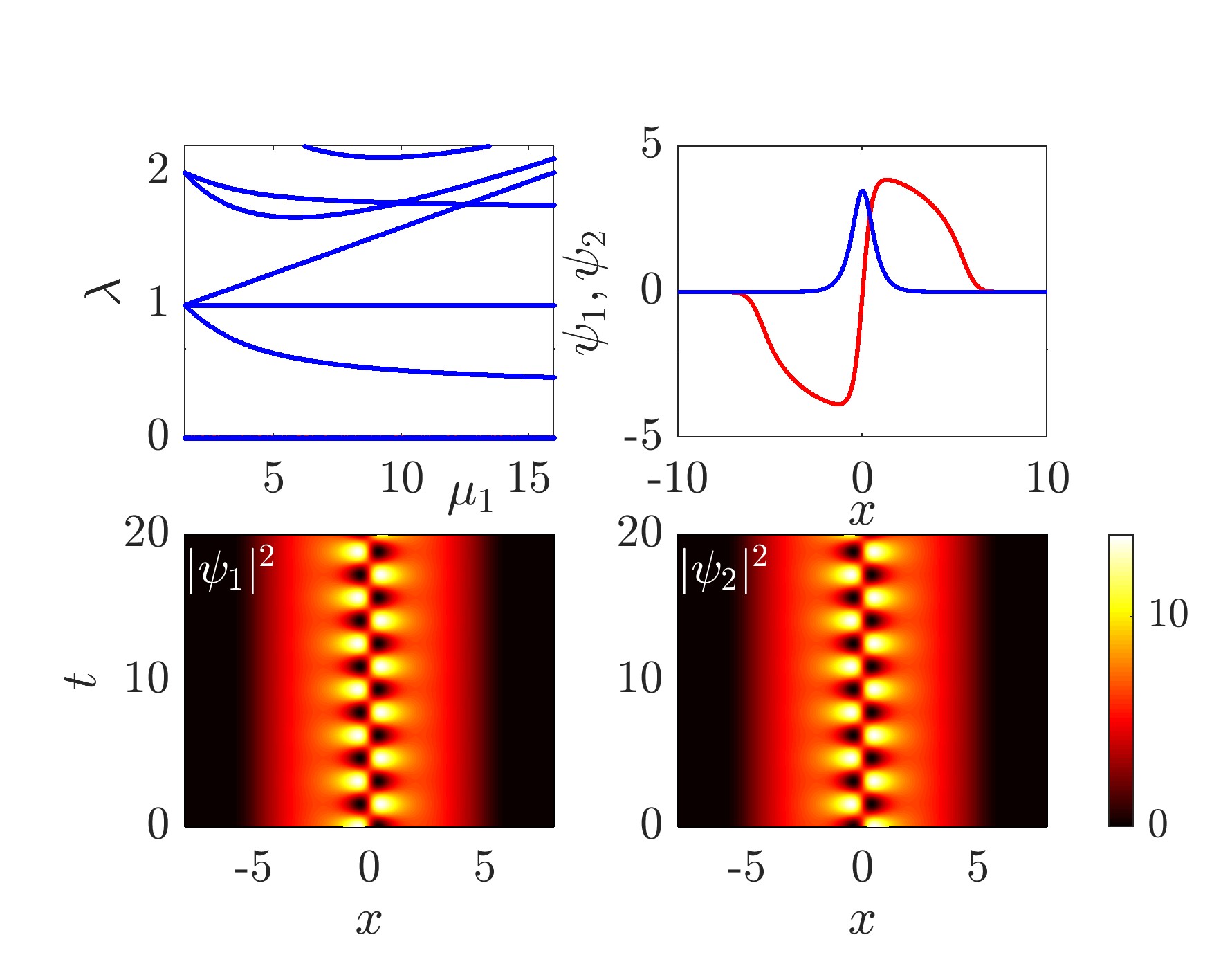
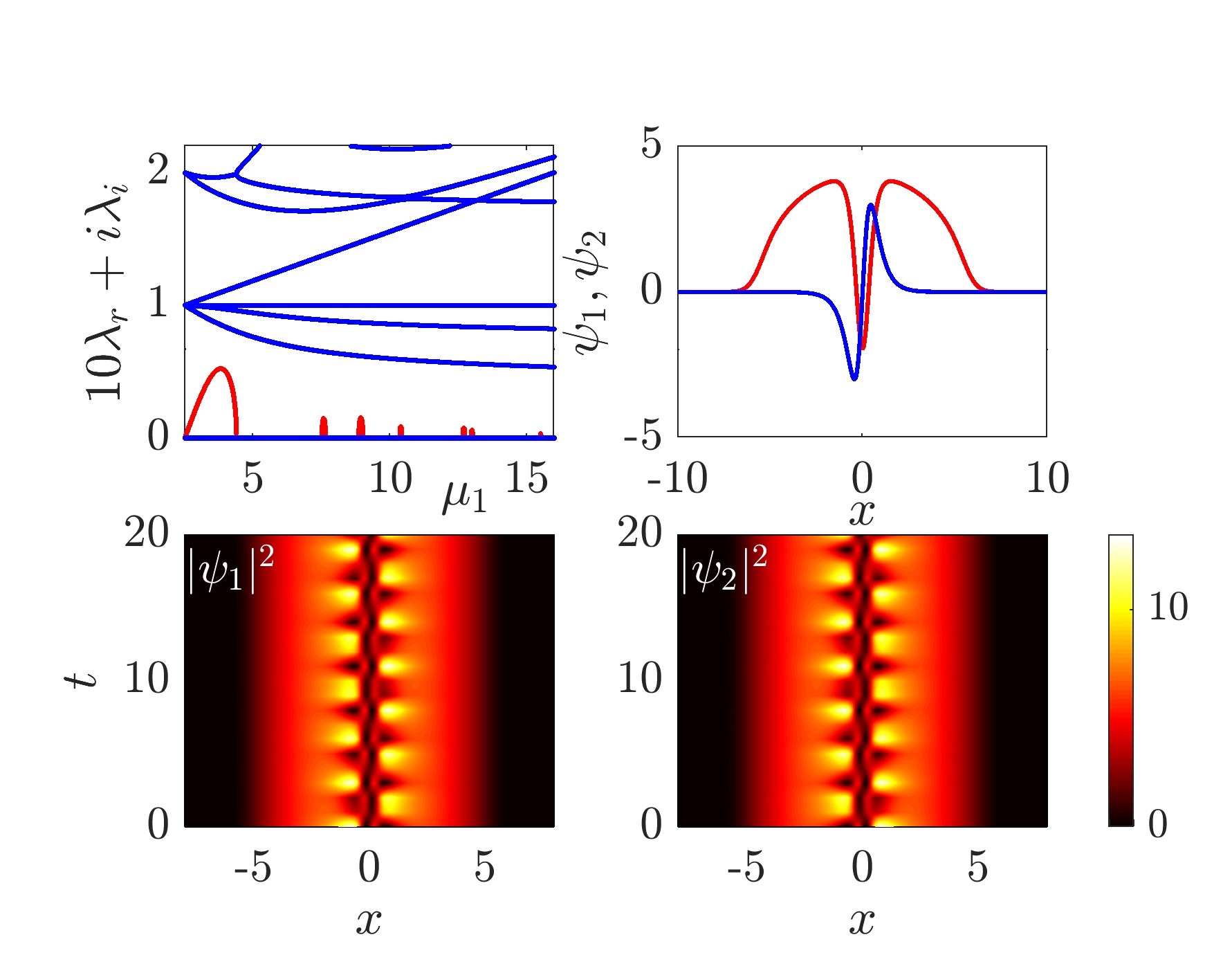
Figure 1: (Color online) Left panel: The BdG stability spectrum of the DB soliton along a linear trajectory from the linear limit $(1.5,0.5$) to a typical large-density limit $(16,14)$ in the $(\mu_{1},\mu_{2})$ parameter space. Red and blue points denote unstable and stable modes, respectively. The stationary DB profile at the end of the parametric line are illustrated, along with the induced DD oscillating patterns. I.e., the DB pattern is SO$(2)$-rotated and fed into the time evolution dynamics in order to observe this dynamical phenomenology. Here and in the contour plots that will follow throughout the manuscript, the density ($|\psi_{i}|^{2}$, $i=1,2$) will be shown for the different components as a function of space and time. The DB, as well as its rotated variant are fully stable and robust. Middle and right panels: Same as the left panel, but for the $\mathcal{S}_{2m}$ family from the linear limit $(2.5,m+0.5$) to a typical large-density limit $(16,14)$. The bright solitons are in phase for $m=0$ and out of phase for $m=1$, the in-phase two-DB state is fully stable, but the out-of-phase one has several (here seven) weak instability peaks. Note that the real part of the eigenvalues for $\mathcal{S}_{21}$ is enlarged by a factor of $10$ for visualization purposes, i.e., the maximum growth rate is approximately $0.5/10=0.05$. All of the breathing patterns in this work are integrated and found to be robust up to $t=1000$.

Next, we focus on the $\mathcal{S}_{3m}$ family as shown in Fig. 2. In this family, all the states considered bear unstable modes; in fact all the states have at least 3 potentially unstable modes because of $n=3$. Furthermore, the number of potential instabilities grows with $m$. In this context, it is reasonable to expect that for states $\mathcal{S}_{nm}$, the maximal number of potentially unstable eigendirections is $n+m$. However, it is important to emphasize that there are again wide ranges of stability. The associated instability bubbles will bear quite small growth rates, especially so in the exception of the first one associated with resonances emerging for small chemical potentials (particle numbers) right off of the linear limit. From a structural perspective, we can observe in the corresponding configurations that each of the DBs is converted, as a result of the transformation, into a DD structure. On the other hand, a DD remains a DD when a collocated DD state exists, as in the case of $\mathcal{S}_{31}$ where the relevant zero crossing will be preserved even after the SO$(2)$ rotation. Similar features to the above ones can be detected for the $\mathcal{S}_{4m}$ family as shown in Fig. 3. Here, again the $\mathcal{S}_{40}$ state is the one that features the smallest number of instability bubbles, although it is relevant to note that off of the linear limit both the $\mathcal{S}_{40}$ and the $\mathcal{S}_{43}$ state feature two such bubbles (while $\mathcal{S}_{41}$ and $\mathcal{S}_{42}$ have only one associated instability). Nevertheless, all selected states at the DB level when dynamically robust, upon their SO$(2)$ rotation yield a number of stable internal vibrations as manifested in the corresponding dynamical evolutions in the bottom sets of space-time contours within the Figs. 2 and 3.

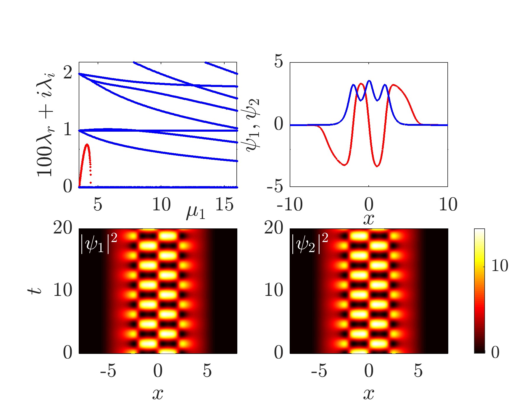
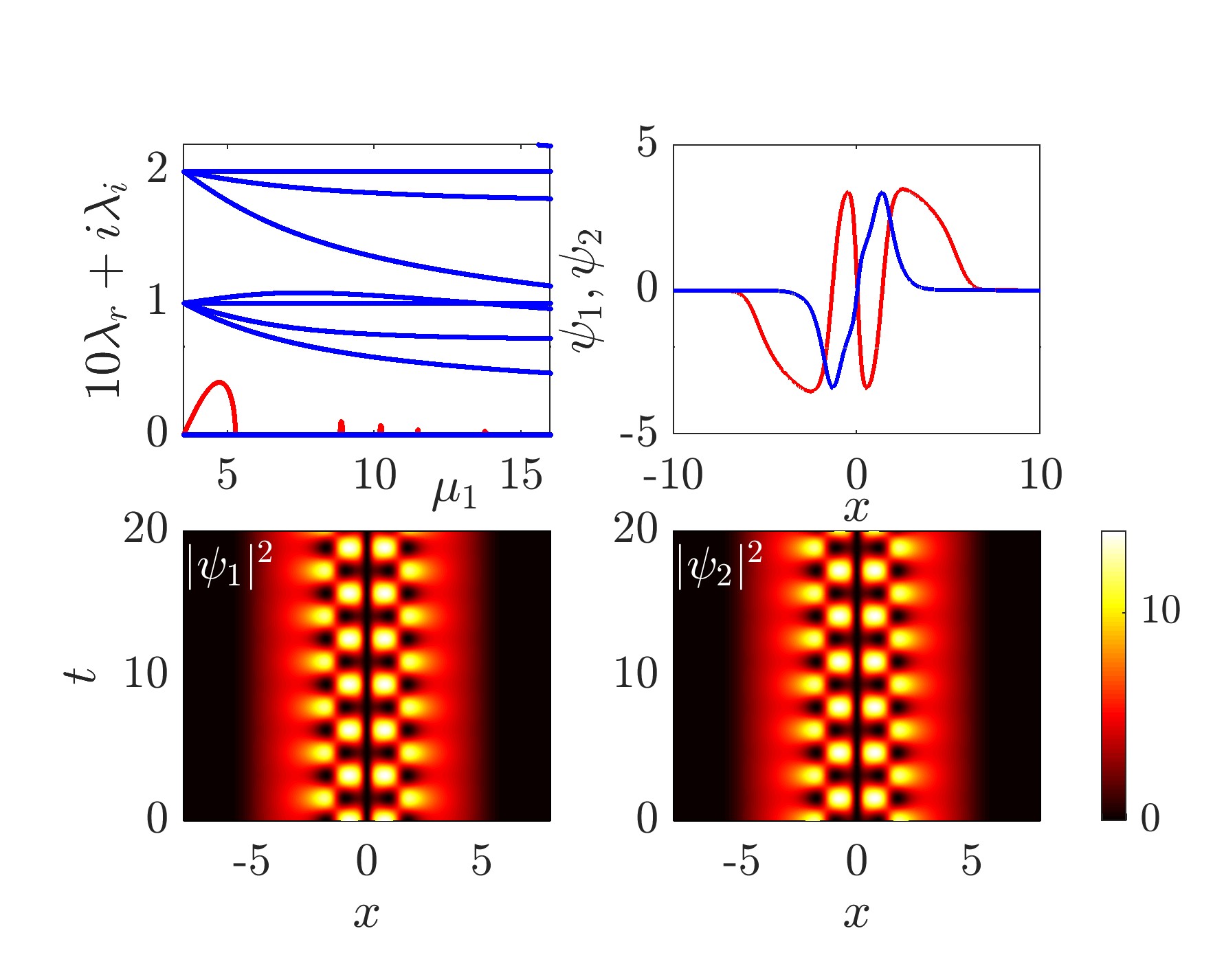
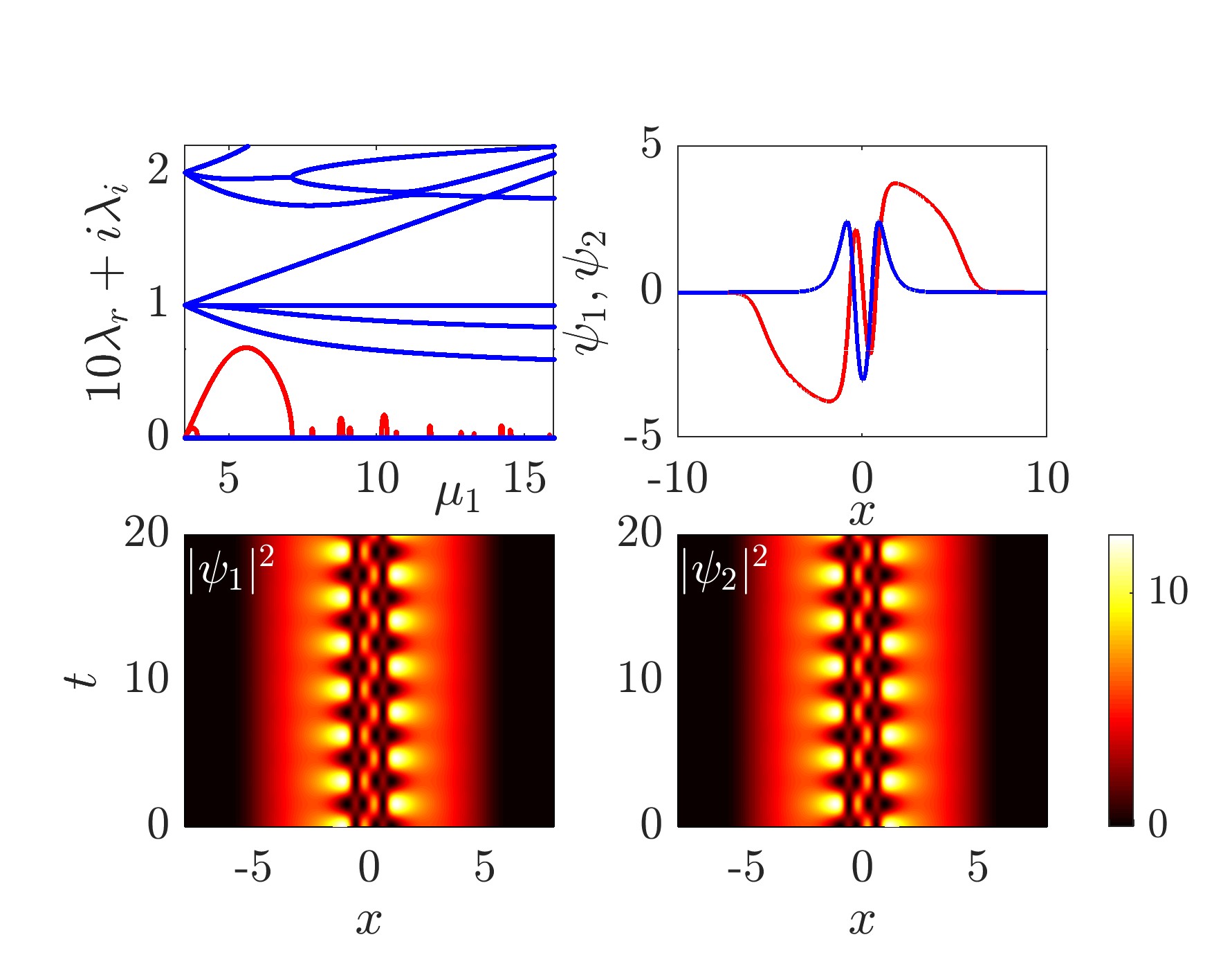
Figure 2: (Color online) Same as Fig. 1, but for the $\mathcal{S}_{3m}$ family from the linear limits $(3.5,m+0.5$) to a typical large-density limit $(16,14)$ in the $(\mu_{1},\mu_{2})$ parameter space. Here, even the in-phase state has an unstable mode, although it is rather weak. The states get progressively more unstable as $m$ increases, i.e., as the number of dark soliton increases in the second component. Note that the second state $\mathcal{S}_{31}$ consists of a DB (left end), DD (middle), and DB (right end) structure.

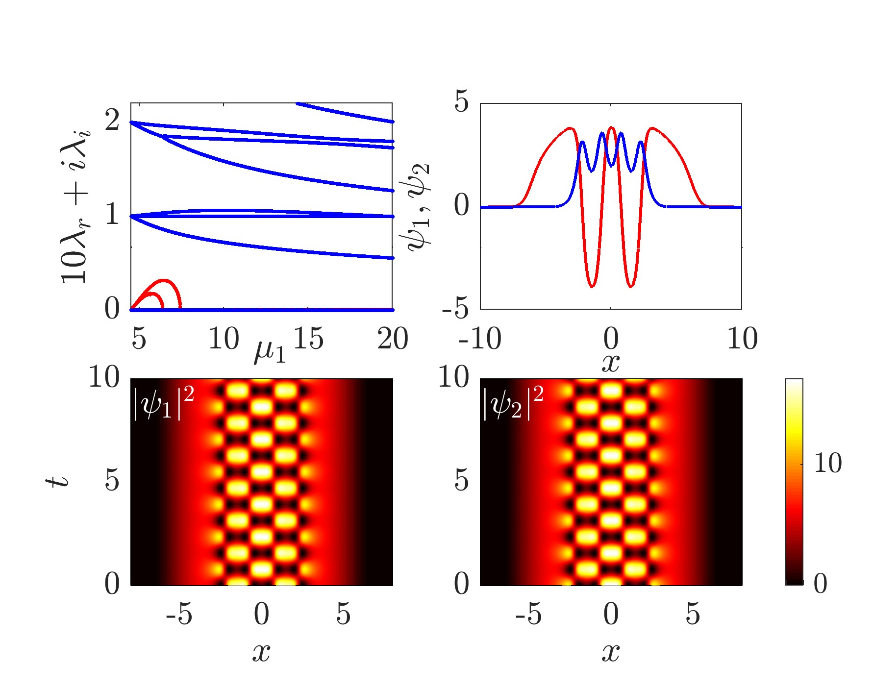
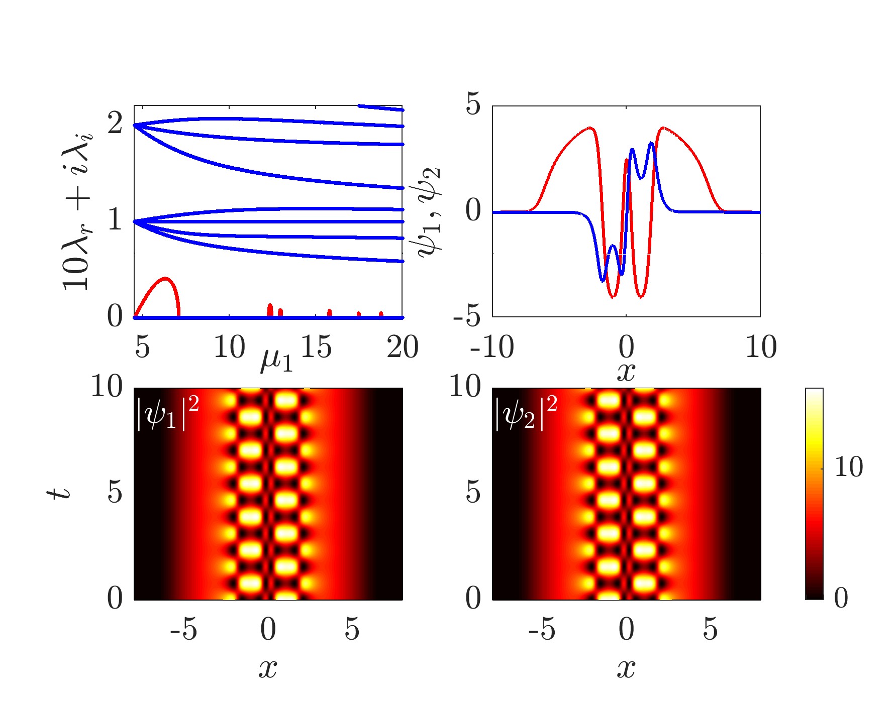
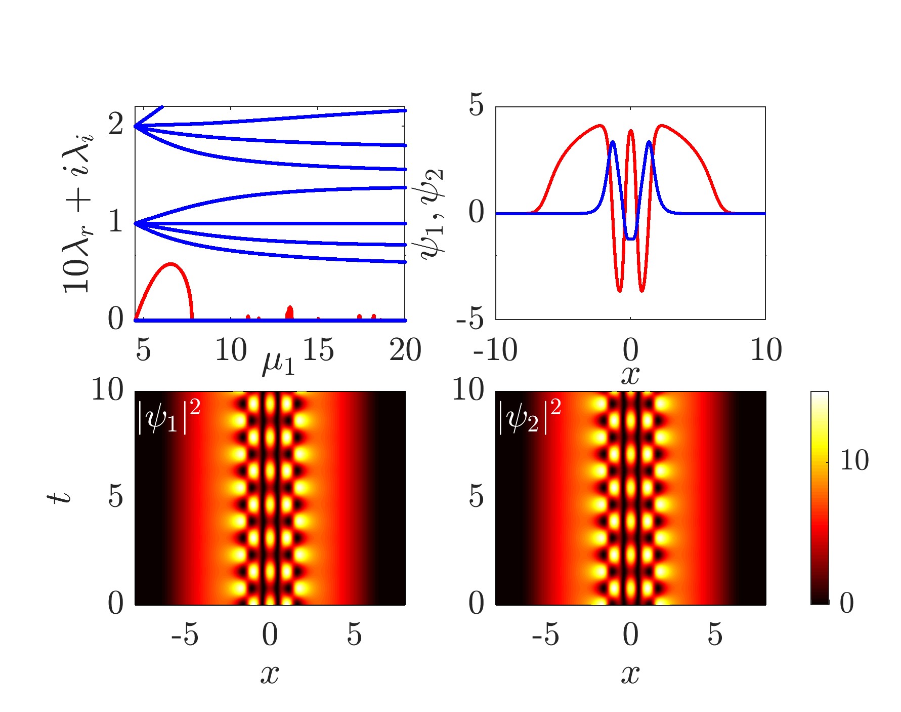
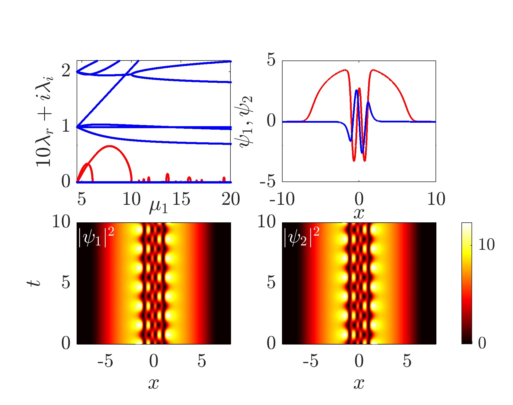
Figure 3: (Color online) Same as Fig. 1, but for the $\mathcal{S}_{4m}$ family from the linear limits $(4.5,m+0.5$) and up to a typical large-density limit $(20,16)$ in the $(\mu_{1},\mu_{2})$ parameter space. The top left quartet of panels concerns the $\mathcal{S}_{40}$ state, the top right the $\mathcal{S}_{41}$ configuration, while, respectively, the bottom left and right constitute the $\mathcal{S}_{42}$ and $\mathcal{S}_{43}$ states. In this case too, the initial conditions obtained as a result of the SO$(2)$ rotations lead to robust breathing states.

Motivated by this observation, we next only look at $\mathcal{S}_{n0}$ states for $n=5,6,...,10$. The results are presented in Figs. 4-5. Naturally, per the above observations, and in line with the results of Kevrekidis et al. (2015), the number of unstable modes, stemming from the linear limits, increases by one whenever a dark soliton is added to the first component. This trend makes it challenging to stabilize multiple dark-bright solitons. Indeed, for the $\mathcal{S}_{10,0}$ state, we need chemical potentials of the order of $100$ to fully stabilize this structure. However, for these sufficiently high values of the chemical potential, our direct numerical simulations confirm the presence of breathing rotated states with a large number of DD structures which lead to the corresponding internal vibrations and the associated breathing patterns. Since such initial conditions have been realized in the recent experiments of Katsimiga et al. (2020), it should, in principle, be possible to visualize and resolve the relevant dynamics.

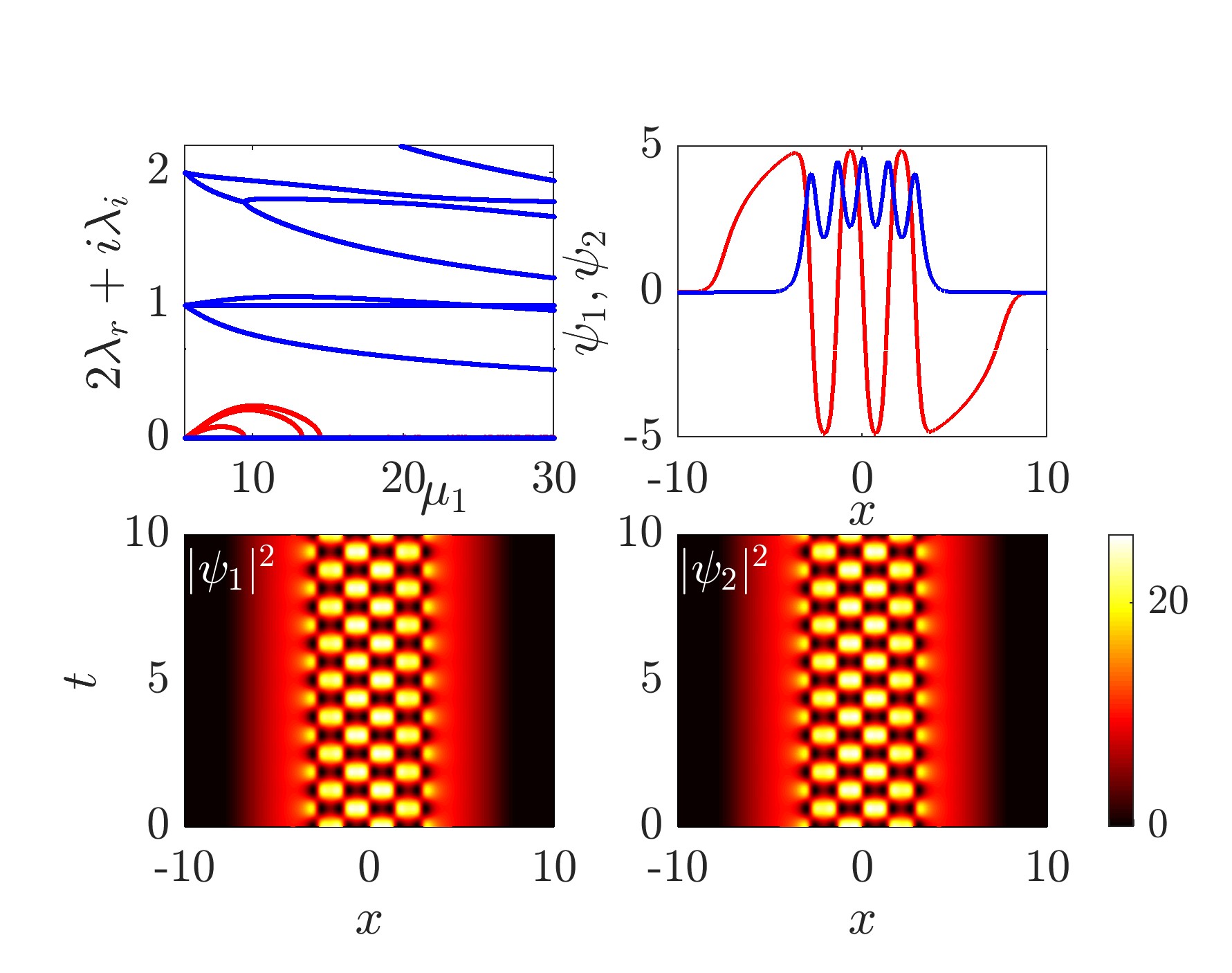
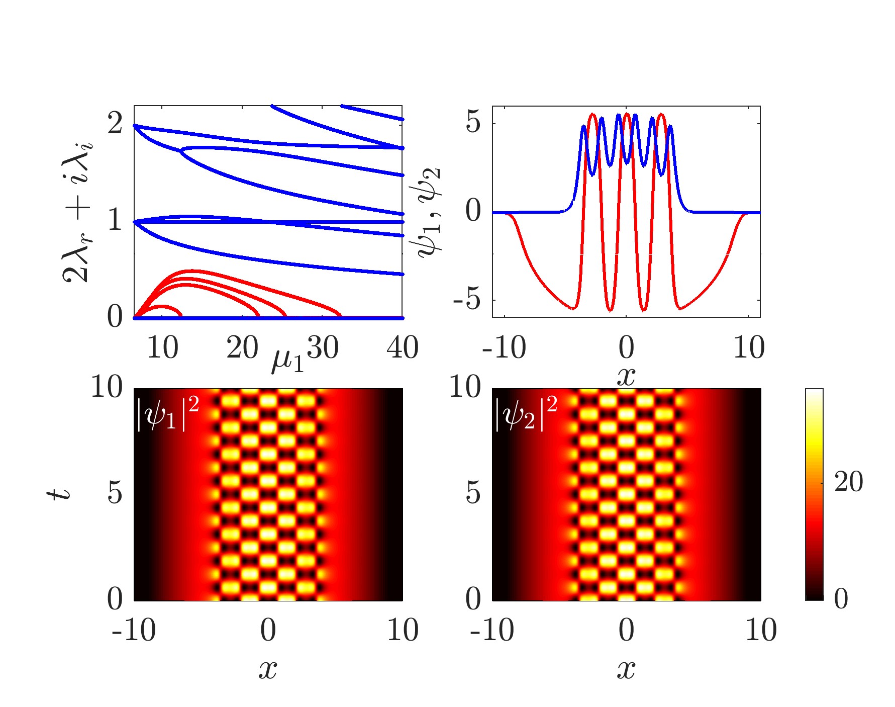
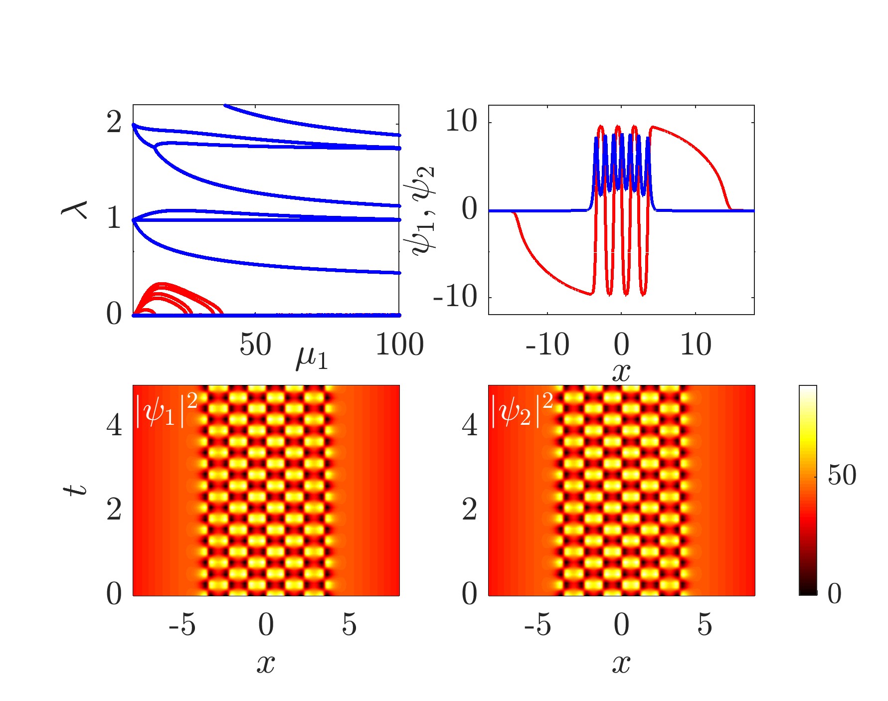
Figure 4: (Color online) Same as Fig. 1, but for the $\mathcal{S}_{n0}$ states from the linear limits $(n+0.5,0.5$) to typical large-density limits. The final chemical potentials are $(30,25)$, $(40,35)$, $(100,88)$ for $n=5,6$, and $7$, respectively. Note that the number of unstable modes increases by $1$ as $n$ increases by $1$.

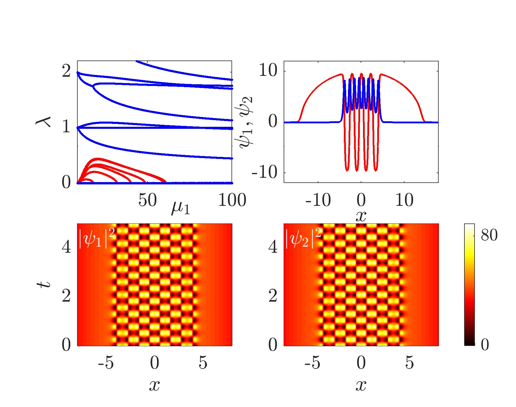
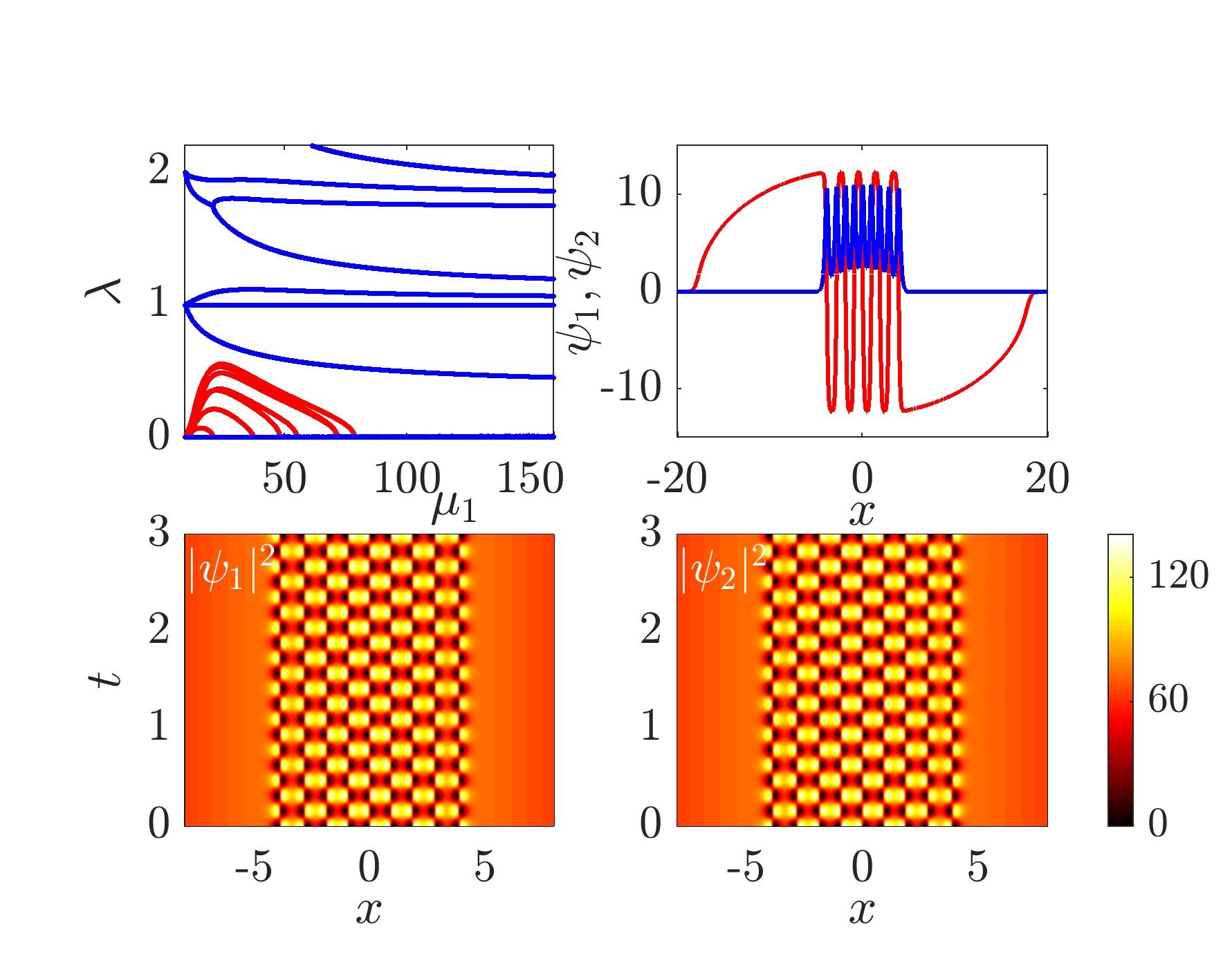
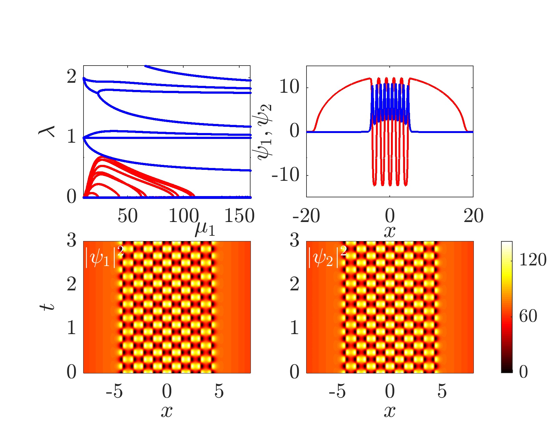
Figure 5: (Color online) Same as Fig. 1, but for the $\mathcal{S}_{80}$, $\mathcal{S}_{90}$, and $\mathcal{S}_{10,0}$ states from the linear limits to $(100,88)$, $(160,140)$, $(160,140)$, respectively. The number of unstable modes continues to grow by one as the number of dark soliton grows by one, upon examining the closely spaced unstable modes. Note that $10$ DB solitons require as large as $\mu_{1}\approx 100$ to be fully stabilized.

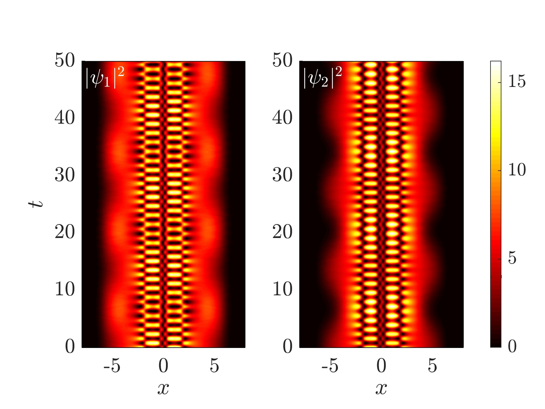
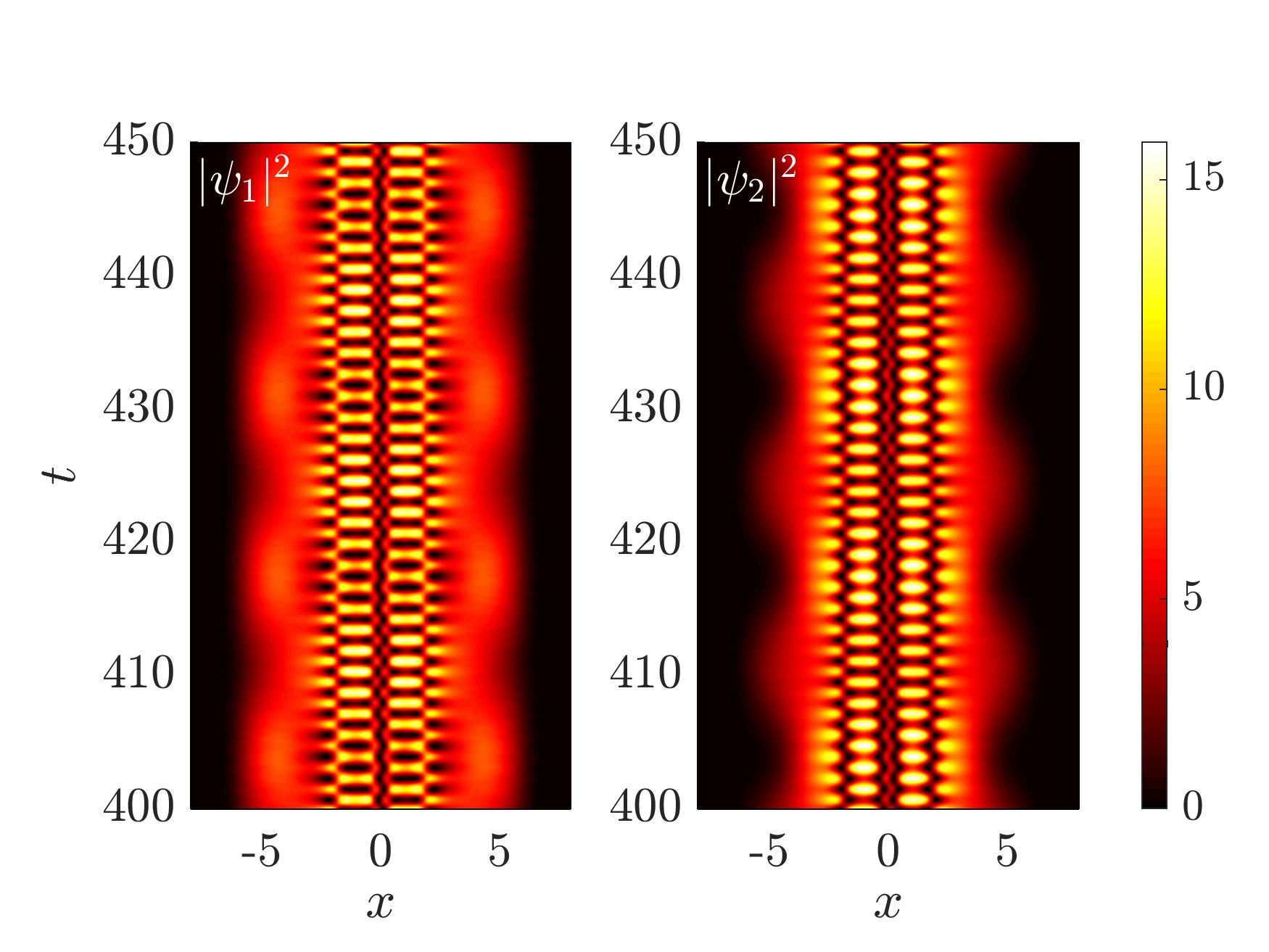
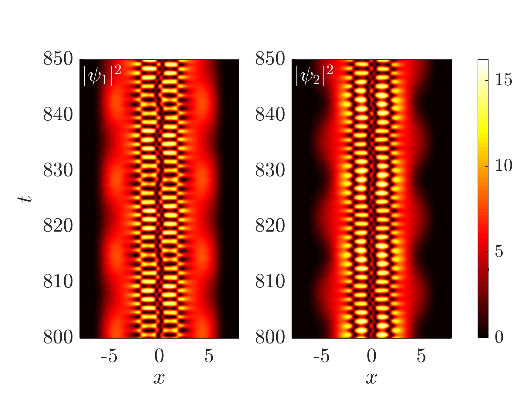
Figure 6: (Color online) Weak disorder for few solitons caused by slight deviations from the perfectly symmetric Manakov limit using the experimentally relevant values $g_{11}=1.03$, $g_{22}=0.97$, and $g_{12}=g_{21}=1$ Yan et al. (2011). Here, the breathing patterns emanating from the $\mathcal{S}_{41}$ state are illustrated, where the stable dynamics is suddenly subjected to the above interaction parameters starting from $t=0$. Note that the ground state breathing mode is immediately excited, and the two condensates breathe in a correlated manner; see the boundary undulation of the condensates. The DD soliton breathing mode is finally also excited (around $t=700$) and the breathing patterns become distorted. Nevertheless, the DD soliton breathing patterns remain robust for several hundred periods before getting disordered.

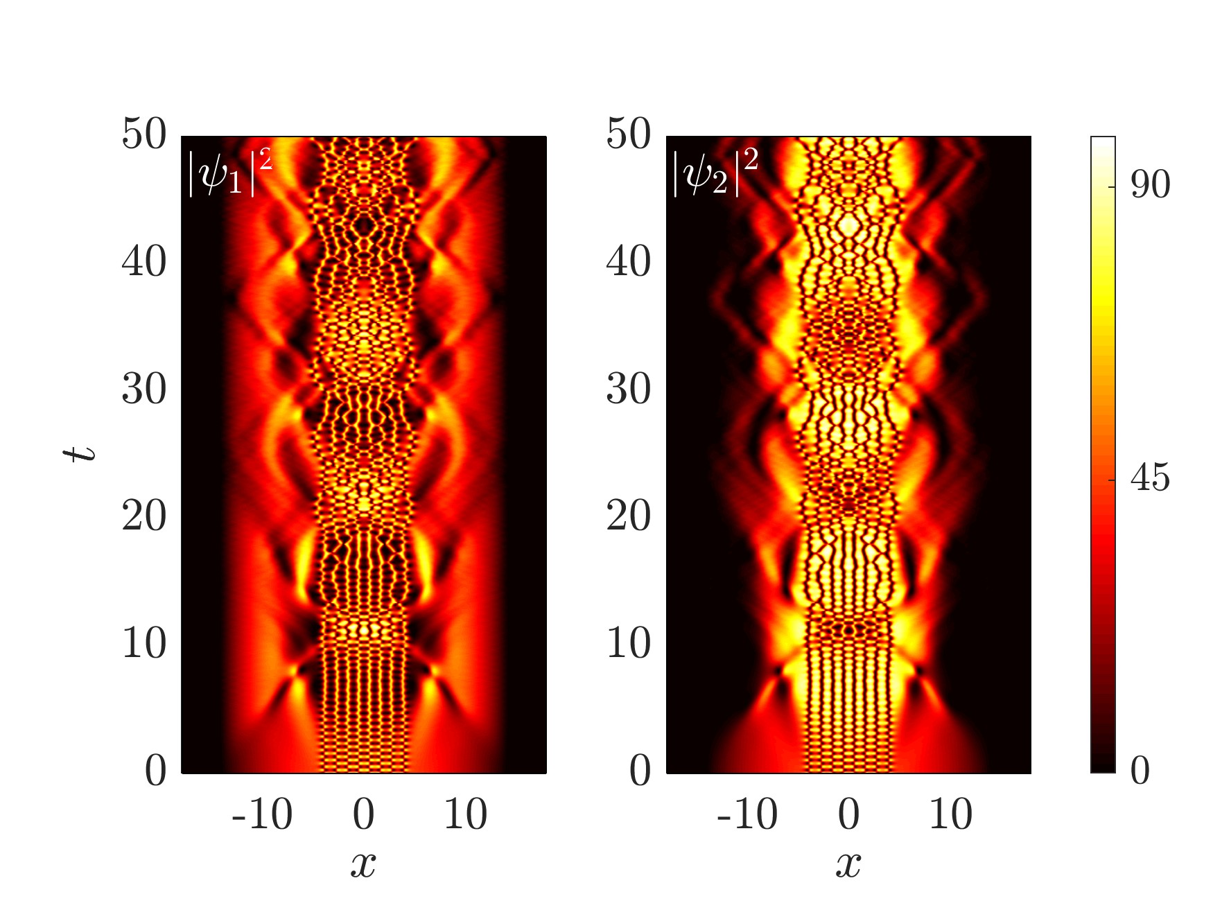
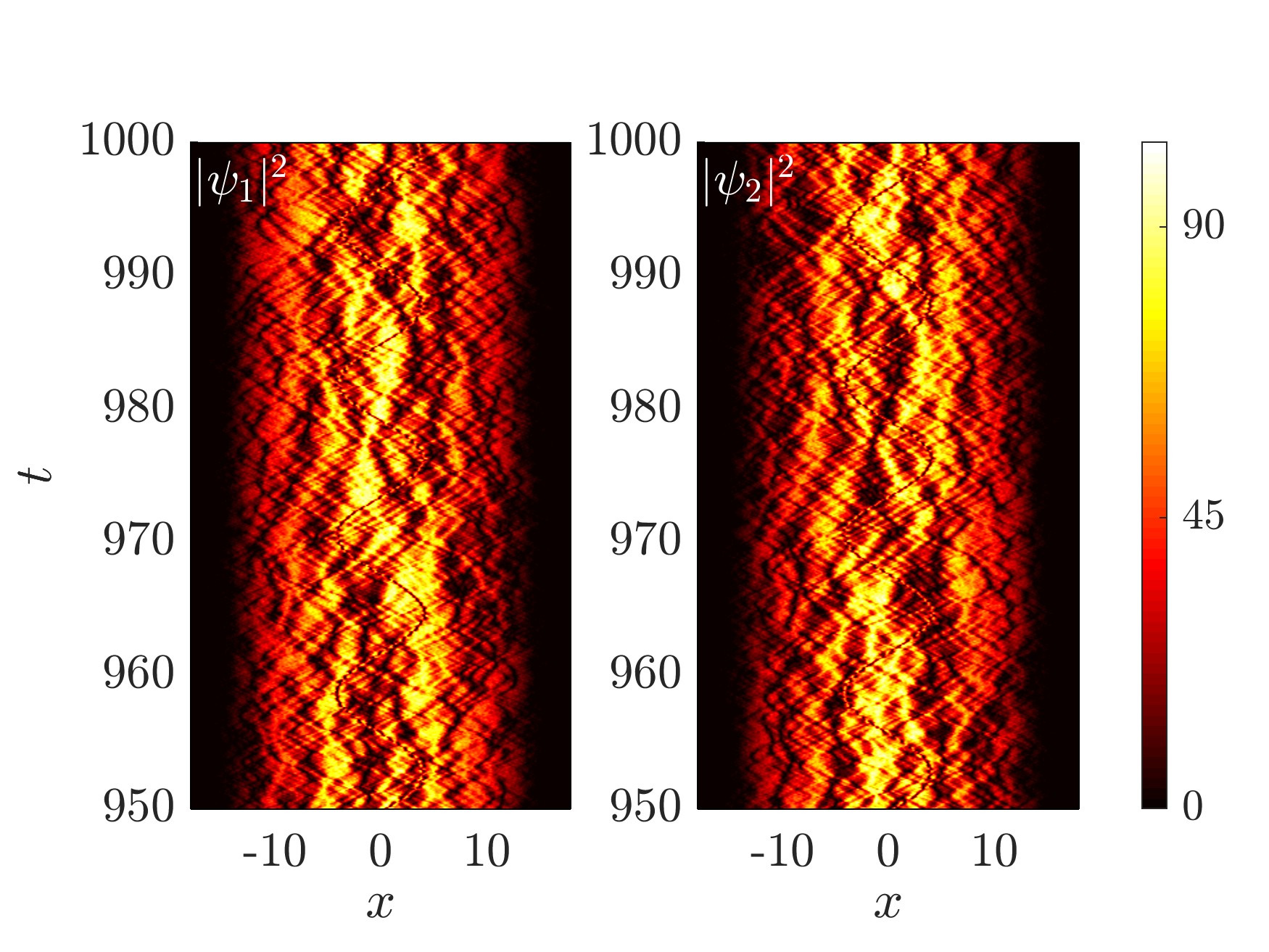
Figure 7: (Color online) Same as Fig. 6 but for breathing patterns emanating from the $\mathcal{S}_{80}$ state. From about $t=10$ onwards, the dark soliton “lattice” gradually undergoes a transition towards a “gaseous” state. In this state, the dark solitons frequently collide, thus generating dark bands in the density profiles. In addition, the background becomes highly excited and fragmented. See the text for more details.

Finally, we study the effects of weak deviations from the perfectly symmetric Manakov limit using the experimentally relevant values $g_{11}=1.03$, $g_{22}=0.97$, and $g_{12}=g_{21}=1$ Mertes et al. (2007); Yan et al. (2011). In particular, Fig. 6 illustrates the breathing patterns corresponding to the $\mathcal{S}_{41}$ state, where the stable dynamics is suddenly subjected to the above interaction parameters starting from $t=0$ (i.e., a quench to the above values of the interaction coefficients). Note that the ground state breathing mode is immediately excited, and the two condensates breathe in a correlated (out of phase) manner; see the relevant condensate boundaries. A DD soliton breathing mode is finally also excited (around $t=700$) and the breathing patterns become distorted. Nevertheless, the soliton breathing patterns remain robust for several hundred periods before getting disordered. Similar behaviour is found for other patterns, where some patterns persist for somewhat shorter periods (e.g. patterns resulting from $\mathcal{S}_{21}$ and $\mathcal{S}_{30}$) and others remain robust for a much larger number of periods (e.g. patterns resulting from $\mathcal{S}_{31}$ and $\mathcal{S}_{40}$).

Strong disorder can manifest quickly and in a pronounced manner for many solitons for the same parameters. A typical time evolution for the state $\mathcal{S}_{80}$ is shown in Fig. 7. In addition to the aforementioned weak disorder, the dark “lattice” in each component can quickly evolve from a more “crystalline” into a “gaseous” state (in line with the terminology of Wang and Kevrekidis (2015)), where the synchronization of the DD soliton vibrations is gradually lost. The states then become so disordered that there is no clearly discernible stationary or periodic pattern. Indeed, dark solitons in the two components frequently collide forming some “dark bands” in the density profile. The backgrounds of both states are also highly excited with this phenomenology persisting up to the time horizon of the very long evolution simulations shown in Fig. 7.

III.2 Multiple dark-dark soliton breathing patterns in a homogeneous setting

The model with no external trap is an integrable Manakov model Manakov (1974), and various types of solitons have been deduced using the traditional inverse scattering method, Bäcklund transformation method, and Hirota bilinear method V. B. Matveev and M. A. Salle (1991); E. V. Doktorov and S. B. Leble (2007); Hirota (2004); Kanna and Lakshmanan (2001); Ling et al. (2015), such as bright-bright (BB), DB and DD solitons. The DB soliton solutions have been extensively investigated Busch and Anglin (2001); Rajendran et al. (2009); Dean et al. (2013); Hamner et al. (2011); Yan et al. (2011); Karamatskos et al. (2015); Katsimiga et al. (2018). Recently, a modified Darboux transformation method focusing towards dark and DB solitary waves in repulsively interacting BECs was developed Ling et al. (2015). Upon use this method to identify the multi-DB soliton solutions, here we focus on the breathing variants thereof arising through SO$(2)$ rotations. The analytical expressions are similar to the ones developed in the above mentioned earlier works, therefore we do not present them in detail.

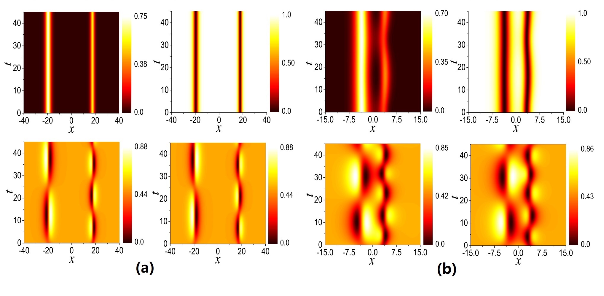
Figure 8: (Color online) Space-time density evolutions of two DB solitons and DD breathing patterns for well-separated (a) and closely initialized (b) cases. The top panels show the bright-soliton component and the dark-soliton component, and the lower panels show the rotated DD breathing patterns. The well-separated solitons yield effectively isolated beating dark-dark solitons, while the nonlinear interaction between solitons changes the beating patterns significantly.

Two typical quasi-static solutions along with the symmetric SO(2) rotated solutions are depicted in Fig. 8 where the panel (a) of the figure shows the evolution of two well-separated DB solitons; essentially these waves are sufficiently far away from each other and, hence, do not feel the presence of each other over the time scale of the simulation. As a result, over the horizon of the simulation shown in panel (a) of Fig. 8, the internal beating of each of the two DD solitary waves occurs with different frequencies. When the solitons are initialized closer, the interaction between them changes the beating patterns as illustrated in Fig. 8(b). Similarly, the cases for three DB solutions and the rotated dynamics are shown in Fig. 9. Fig. 9(a) shows the evolution of three well-separated DB solitons, again with very distinct breathing frequencies. As the initial DBs are brought closer, the beating patterns again become strongly affected by the interaction between solitons; cf. Fig. 8(b). These beating patterns are found to be stable against weak perturbations. The resulting pattern while highly dynamical remains spatially localized, while this would no longer be true due to modulational instability of the density background in the attractive case Zhao et al. (2019).

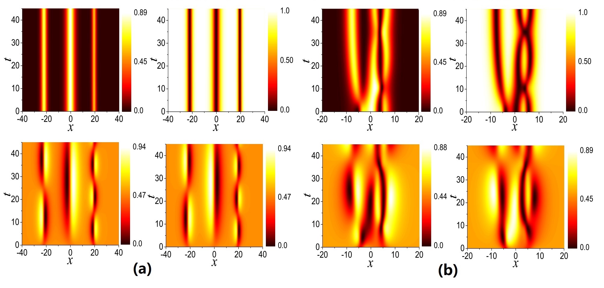
Figure 9: (Color online) Similar to the previous figure but now for the 3 dark-bright soliton case, once again when well-separated (a) and nonlinearly interacting (b).

III.3 Three-component dark-dark-dark breathing patterns

In the last section of our present work, we turn our focus to the three-component case. In particular, the GPEs can be generalized to the following system:

$$i\frac{\partial\psi_{1}}{\partial t} =-\frac{1}{2}\frac{\partial^{2}\psi_{1}}{\partial x^{2}}+\left(g_{11}|\psi_{1}|^{2}+g_{12}|\psi_{2}|^{2}+g_{13}|\psi_{3}|^{2}\right)\psi_{1}+V(x)\psi_{1},$$ (7a)

$$i\frac{\partial\psi_{2}}{\partial t} =-\frac{1}{2}\frac{\partial^{2}\psi_{2}}{\partial x^{2}}+\left(g_{21}|\psi_{1}|^{2}+g_{22}|\psi_{2}|^{2}+g_{23}|\psi_{3}|^{2}\right)\psi_{2}+V(x)\psi_{2},$$ (7b)

$$i\frac{\partial\psi_{3}}{\partial t} =-\frac{1}{2}\frac{\partial^{2}\psi_{3}}{\partial x^{2}}+\left(g_{31}|\psi_{1}|^{2}+g_{32}|\psi_{2}|^{2}+g_{33}|\psi_{3}|^{2}\right)\psi_{3}+V(x)\psi_{3},$$ (7c)

where $\psi_{j}(x,t)$ ($j=1,2,3$) are similarly the macroscopic wavefunctions and $g_{ij}$ ($i,j=1,2,3$) are the interaction coefficients with $g_{21}\equiv g_{12}$, $g_{31}\equiv g_{13}$, $g_{32}\equiv g_{23}$. Note that we will explore the Manakov case herein corresponding to $g_{ij}=1$. As discussed in the introduction, in addition to its mathematical interest, this scenario has been touched upon in nonlinear optical multi-component settings; a corresponding BEC framework would also need to incorporate the spin-dependent aspect of interactions within the spinor condensates Kawaguchi and Ueda (2012); Stamper-Kurn and Ueda (2013). The Manakov setting features an SU$(3)$ symmetry of the system. The external potential assumes the same parabolic form of $V(x)=\left(1/2\right)\omega^{2}x^{2}$ with $\omega=1$. Consequently, stationary states can be constructed by assuming

$$\psi_{j}(x,t)=\psi^{0}_{j}(x)e^{-i\mu_{j}t}$$ (8)

which transform Eqs. (7a)-(7c) into the steady-state system:

$$-\frac{1}{2}\frac{d^{2}\psi_{1}^{0}}{dx^{2}}+\left(g_{11}|\psi_{1}^{0}|^{2}+g_{12}|\psi_{2}^{0}|^{2}+g_{13}|\psi_{3}^{0}|^{2}\right)\psi_{1}^{0}+V(x)\psi_{1}^{0}-\mu_{1}\psi_{1}^{0} =0,$$ (9a)

$$-\frac{1}{2}\frac{d^{2}\psi_{2}^{0}}{dx^{2}}+\left(g_{12}|\psi_{1}^{0}|^{2}+g_{22}|\psi_{2}^{0}|^{2}+g_{23}|\psi_{3}^{0}|^{2}\right)\psi_{2}^{0}+V(x)\psi_{2}^{0}-\mu_{2}\psi_{2}^{0} =0,$$ (9b)

$$-\frac{1}{2}\frac{d^{2}\psi_{3}^{0}}{dx^{2}}+\left(g_{13}|\psi_{1}^{0}|^{2}+g_{23}|\psi_{2}^{0}|^{2}+g_{33}|\psi_{3}^{0}|^{2}\right)\psi_{3}^{0}+V(x)\psi_{3}^{0}-\mu_{3}\psi_{3}^{0} =0,$$ (9c)

that we solve numerically. The computational set up is similar to the two-component case, tracing states from their linear limits to a Thomas-Fermi regime. For completeness, the BdG stability analysis is presented in the Appendix. It is also relevant to mention that restricting this matrix to its $4\times 4$ submatrix of the top left elements and setting $\psi_{3}=0$, one retrieves naturally as a special case the corresponding 2-component BdG stability matrix. Since our goal is to illustrate the generality of our method, we will only examine in detail here two prototypical examples, namely the low-lying $\mathcal{S}_{210}$ and $\mathcal{S}_{310}$ states.

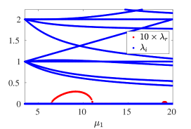
Figure 10: (Color online) The BdG spectra ($\lambda=\lambda_{r}+i\lambda_{i}$) for the states $\mathcal{S}_{210}$ (left) and $\mathcal{S}_{310}$ (right) as a function of $\mu_{1}$. Here, the states emanate from the linear limits and our continuation terminates close to a TF regime with $(\mu_{1},\mu_{2},\mu_{3})=(20,18,16)$. Note that both states feature wide intervals of stability. The real parts in both panels are multiplied by a factor of $10$ for visualization purposes.

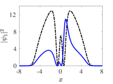
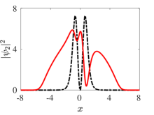
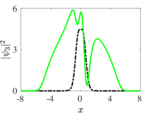
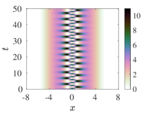
Figure 11: (Color online) Summary of results for the $\mathcal{S}_{210}$ state. Top row: The densities $|\psi_{j}|^{2}$ ($j=1,2,3$) of the steady-state profiles for $\mu_{1}=14.998146$, $\mu_{2}=13.284432$, and $\mu_{3}=11.570432$ are shown with dashed-dotted black lines, and the SU$(3)$ rotated versions of them are shown with solid blue, red, and green lines, respectively. Bottom row: Spatio-temporal evolutions of the densities $|\psi_{1}(x,t)|^{2}$ (left panel), $|\psi_{2}(x,t)|^{2}$ (middle panel), and $|\psi_{3}(x,t)|^{2}$ (right panel) are shown where the initial states employed are the SU$(3)$ rotated states of the top row.

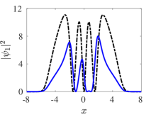
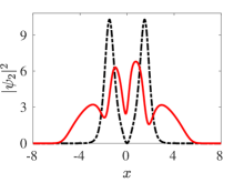
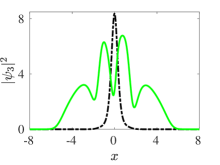
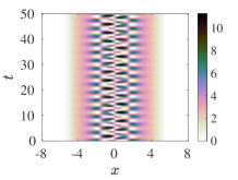
Figure 12: (Color online) Same as Fig. 11 but for the $\mathcal{S}_{310}$ state with chemical potentials $\mu_{1}=15.283574$, $\mu_{2}=13.283574$, and $\mu_{3}=11.569574$. Note that there are genuinely two frequencies involved in this dark-dark-dark breathing dynamics.

We perform the continuation of both states $\mathcal{S}_{210}$ and $\mathcal{S}_{310}$ over the chemical potentials from the associated linear limits to a TF regime of $(\mu_{1},\mu_{2},\mu_{3})=(20,18,16)$. The left and right panels of Fig. 10 correspond to the BdG spectra of $\mathcal{S}_{210}$ and $\mathcal{S}_{310}$, respectively. It should be noted that although both branches have intervals of instabilities (see the (red colored) “instability bubbles” in the pertinent panels), there exist wide intervals of stability where the solutions are expected to be long lived. Upon selecting stable steady-states (according to our spectral stability analysis results), we SU$(3)$-rotate them in order to explore the possibility of forming breathing yet robust patterns in the three-component case. Generally, this can be done by means of a unitary matrix $U=e^{iH\theta}$, where $H$ is a linear combination of the so-called Gell-Mann matrices Gell-Mann (1962). To be more specific, we focus on a symmetric rotation dictated by the following unitary matrix Zhao (2018):

$$U=\frac{1}{\sqrt{3}}\left(\begin{array}[]{ccc}1&1&1\\ 1&-\exp(i\pi/3)&\exp(i2\pi/3)\\ 1&\exp(i2\pi/3)&-\exp(i\pi/3)\\ \end{array}\right).$$ (10)

Figures 11 and 12 summarize our results for the $\mathcal{S}_{210}$ and $\mathcal{S}_{310}$, respectively. In particular, the top panels therein showcase the spatial distribution of the densities of the respective components for the unrotated (dashed-dotted lines) and rotated (solid lines) solutions. The bottom panels in the figures offer the spatio-temporal evolution of the subsequent dark-dark-dark beating patterns ($|\psi_{1}(x,t)|^{2}$, $|\psi_{2}(x,t)|^{2}$, and $|\psi_{3}(x,t)|^{2}$ are shown from left to right). Naturally, there are two dark solitons in each component for the rotated $\mathcal{S}_{210}$ whereas there exist three for the rotated $\mathcal{S}_{310}$. The beating dynamics of $\mathcal{S}_{210}$ is robustly periodic, featuring a single-period internal vibration of the state. Upon examination, this is a coincidence resulting from our chosen parameters, where $\mu_{1}-\mu_{2}=\mu_{2}-\mu_{3}$, yielding only one period, i.e., $2\pi/(\mu_{1}-\mu_{2})\approx 3.6664$. This agrees very well with the results of our simulations. On the other hand, two frequencies are genuinely present for the $\mathcal{S}_{310}$ beating dynamics, as the above relation has not been selected in our initial data. Beating patterns for the $\mathcal{S}_{210}$ state in the homogeneous setting, i.e., without an external trapping potential, were studied analytically for particular solutions Zhao (2018). However, in the present work, we demonstrate that this state exists and is, in fact, robust over a wide range of parameters.

IV Conclusions and Future Challenges

The present work offered a systematic study of distinct SO$(2)$-induced multiple dark-dark breathing patterns from stationary and stable dark-bright and dark-dark bound modes. In particular, we studied the existence and stability of these structures from their respective linear limits to typical Thomas-Fermi regimes. We found that for $n$ solitons, there are $n$ distinct coherent patterns that stem from the linear limit and which range from fully in-phase to fully out-of-phase ones. Analytical results in the homogeneous setting are also discussed: here the rotation typically involves the breathing of dynamically non-stationary configurations. Moreover, we presented a generalization of our approach to the three-component GPE system to illustrate prototypical case examples showcasing the generality of the considerations discussed herein.

Motivated by this work, there are multiple avenues for future study that we plan to pursue. One natural extension of our work is to generalize considerations to higher dimensions. In 2D, vortex clusters and/or dark soliton filaments filled with bright components of various relative phases are possible, generating, e.g., various vortex cluster-vortex cluster breathing patterns. In 3D, vortex filaments and/or dark soliton surfaces filled with bright components of various relative phases are relevant for future studies. Importantly, recent experimental progress, including, e.g., the configurations reported in Katsimiga et al. (2020), suggests that such states can be accessed as initial conditions in state-of-the-art experiments and hence the corresponding vibrational dynamics should, in principle, be experimentally tractable. It is not readily obvious that one can find a systematic way to construct all the topologically distinct states and breathing patterns as in 1D since new states can bifurcate away from the linear limit E. G. Charalampidis, N. Boullé, P. E. Farrell, and P. G. Kevrekidis (2019). In addition, there are also different possible combinations of linear eigenmodes. For instance, $|1,0\rangle$ (where the separated by comma indices denote here the linear eigenstates in the different spatial dimensions) produces a dark soliton stripe, while $(|1,0\rangle+i|0,1\rangle)/\sqrt{2}$ produces a single vortex, starting from essentially the same basis. An additional challenge concerns the (in)stability properties of these structures. It is relevant to seek suitable potential configurations to stabilize, e.g., some dark soliton filaments and surfaces against their transverse instabilities by adding external pinning potentials. It is also challenging to stabilize certain multiple vortical filament structures, and preliminary data suggest that even the double vortex rings filled by either in-phase or out-of-phase bright components are extremely difficult to stabilize, at least in a spherical trap. In this situation, one can either further increase the chemical potentials or explore instead other trap settings.

Finally, systematic studies of the three-component system and even beyond that are also interesting; notice, in that vein, both the $F=1$ and $F=2$ spinor systems are presently experimentally accessible in atomic condensates Kawaguchi and Ueda (2012); Stamper-Kurn and Ueda (2013). In our work, we have studied a few select examples of three-component structures, focusing, in particular, on the Manakov case. Yet, more complex structures should be accessible under physically realistic (spinor) perturbations, but also in higher dimensions. Research work along these lines are currently in progress, and will be reported in future publications.

Appendix: Linear stability analysis of the three-component GPE

In this Appendix, we discuss about the setup of the stability analysis problem. To this end, we perform a BdG stability analysis of a steady-state solution $\psi_{j}^{0}(x)$ by introducing the following perturbation Ansätze:

$$\widetilde{\psi}_{j}(x,t)=e^{-i\mu_{j}t}\Big{\{}\psi_{j}^{0}(x)+\varepsilon\left(a_{j}(x)e^{\lambda t}+b_{j}^{\ast}(x)e^{\lambda^{\ast}t}\right)\Big{\}},\quad j=1,2,3,$$ (11)

where $\varepsilon\ll 1$. Upon substituting Eq. (11) into Eqs. (7a)-(7c), we obtain at order $O(\varepsilon)$ an eigenvalue problem of the form:

$$\rho\begin{pmatrix}a_{1}\\ b_{1}\\ a_{2}\\ b_{2}\\ a_{3}\\ b_{3}\end{pmatrix}=\begin{pmatrix}A_{11}&A_{12}&A_{13}&A_{14}&A_{15}&A_{16}\\ -A_{12}^{\ast}&-A_{11}&-A_{14}^{\ast}&-A_{13}^{\ast}&-A_{16}^{\ast}&-A_{15}^{\ast}\\ A_{13}^{\ast}&A_{14}&A_{33}&A_{34}&A_{35}&A_{36}\\ -A_{14}^{\ast}&-A_{13}&-A_{34}^{\ast}&-A_{33}&-A_{36}^{\ast}&-A_{35}^{\ast}\\ A_{15}^{\ast}&A_{16}&A_{35}^{\ast}&A_{36}&A_{55}&A_{56}\\ -A_{16}^{\ast}&-A_{15}&-A_{36}^{\ast}&-A_{35}&-A_{56}^{\ast}&-A_{55}\end{pmatrix}\begin{pmatrix}a_{1}\\ b_{1}\\ a_{2}\\ b_{2}\\ a_{3}\\ b_{3}\end{pmatrix},$$ (12)

where the distinct matrix elements are given by:

$$A_{11} =-\frac{1}{2}\frac{d^{2}}{dx^{2}}+2g_{11}|\psi_{1}^{0}|^{2}+g_{12}|\psi_{2}^{0}|^{2}+g_{13}|\psi_{3}^{0}|^{2}+V(x)-\mu_{1},$$

$$A_{12} =g_{11}\left(\psi^{0}_{1}\right)^{2},$$

$$A_{13} =g_{12}\psi_{1}^{0}\left(\psi_{2}^{0}\right)^{\ast},$$

$$A_{14} =g_{12}\psi_{1}^{0}\psi_{2}^{0},$$

$$A_{15} =g_{13}\psi_{1}^{0}\left(\psi_{3}^{0}\right)^{\ast},$$

$$A_{16} =g_{13}\psi_{1}^{0}\psi_{3}^{0},$$

$$A_{33} =-\frac{1}{2}\frac{d^{2}}{dx^{2}}+g_{12}|\psi_{1}^{0}|^{2}+2g_{22}|\psi_{2}^{0}|^{2}+g_{23}|\psi_{3}^{0}|^{2}+V(x)-\mu_{2},$$

$$A_{34} =g_{22}\left(\psi_{2}^{0}\right)^{2},$$

$$A_{35} =g_{23}\psi_{2}^{0}\left(\psi_{3}^{0}\right)^{\ast},$$

$$A_{36} =g_{23}\psi_{2}^{0}\psi_{3}^{0},$$

$$A_{55} =-\frac{1}{2}\frac{d^{2}}{dx^{2}}+g_{13}|\psi_{1}^{0}|^{2}+g_{23}|\psi_{2}^{0}|^{2}+2g_{33}|\psi_{3}^{0}|^{2}+V(x)-\mu_{3},$$

$$A_{56} =g_{33}\left(\psi_{3}^{0}\right)^{2}.$$

Here, $\rho=i\lambda$ is the eigenvalue with the associated eigenvector:

$$\mathbf{W}(x)=\left(a_{1}(x)\,b_{1}(x)\,a_{2}(x)\,b_{2}(x)\,a_{3}(x)\,b_{3}(x)\right)^{T}.$$

The eigenvalue computations for the three-component case were performed by using the FEAST eigenvalue solver Kestyn et al. (2016) where (usually)  $100$ eigenvalues were computed with $10^{-8}$ tolerance on the residuals.

References

- Pitaevskii and Stringari (2003) L. Pitaevskii and S. Stringari, Bose–Einstein Condensation (Oxford University Press, Oxford, UK, 2003).
- Pethick and Smith (2002) C. Pethick and H. Smith, Bose–Einstein Condensation in Dilute Gases (Cambridge University Press, Cambridge, UK, 2002).
- Kevrekidis et al. (2015) P. G. Kevrekidis, D. J. Frantzeskakis, and R. Carretero-González, The Defocusing Nonlinear Schrödinger Equation: From Dark Solitons to Vortices and Vortex Rings (SIAM, Philadelphia, 2015).
- Kivshar and Luther-Davies (1998) Y. S. Kivshar and B. Luther-Davies, Dark optical solitons: physics and applications, Physics Reports 298, 81 (1998), ISSN 0370-1573.
- Abdullaev et al. (2005) F. Abdullaev, A. Gammal, A. Kamchatnov, and L. Tomio, Dynamics of bright matter wave solitons in a Bose-Einstein condensate, Int. J. Mod. Phys. B 19, 3415 (2005).
- Frantzeskakis (2010) D. J. Frantzeskakis, Dark solitons in atomic Bose–Einstein condensates: from theory to experiments, Journal of Physics A: Mathematical and Theoretical 43, 213001 (2010).
- Fetter and Svidzinsky (2001) A. L. Fetter and A. A. Svidzinsky, Vortices in a trapped dilute Bose-Einstein condensate, Journal of Physics: Condensed Matter 13, R135 (2001).
- Fetter (2009) A. L. Fetter, Rotating trapped Bose-Einstein condensates, Rev. Mod. Phys. 81, 647 (2009).
- Komineas (2007) S. Komineas, Vortex rings and solitary waves in trapped Bose–Einstein condensates, The European Physical Journal Special Topics 147, 133 (2007).
- Proment et al. (2012) D. Proment, M. Onorato, and C. F. Barenghi, Vortex knots in a Bose-Einstein condensate, Phys. Rev. E 85, 036306 (2012).
- Busch and Anglin (2001) T. Busch and J. R. Anglin, Dark-Bright Solitons in Inhomogeneous Bose-Einstein Condensates, Phys. Rev. Lett. 87, 010401 (2001).
- Becker et al. (2008) C. Becker, S. Stellmer, P. Soltan-Panahi, S. Dörscher, M. Baumert, E.-M. Richter, J. Kronjäger, K. Bongs, and K. Sengstock, Oscillations and interactions of dark and dark-bright solitons in Bose-Einstein condensates, Nature Physics 4, 496 (2008).
- Romero-Ros et al. (2019) A. Romero-Ros, G. C. Katsimiga, P. G. Kevrekidis, and P. Schmelcher, Controlled generation of dark-bright soliton complexes in two-component and spinor Bose-Einstein condensates, Phys. Rev. A 100, 013626 (2019).
- Kiehn et al. (2019) H. Kiehn, S. I. Mistakidis, G. C. Katsimiga, and P. Schmelcher, Spontaneous generation of dark-bright and dark-antidark solitons upon quenching a particle-imbalanced bosonic mixture, Phys. Rev. A 100, 023613 (2019).
- Yan et al. (2011) D. Yan, J. J. Chang, C. Hamner, P. G. Kevrekidis, P. Engels, V. Achilleos, D. J. Frantzeskakis, R. Carretero-González, and P. Schmelcher, Multiple dark-bright solitons in atomic Bose-Einstein condensates, Phys. Rev. A 84, 053630 (2011).
- Kevrekidis and Frantzeskakis (2016) P. Kevrekidis and D. Frantzeskakis, Solitons in coupled nonlinear Schrödinger models: A survey of recent developments, Reviews in Physics 1, 140 (2016), ISSN 2405-4283.
- Wang and Kevrekidis (2017) W. Wang and P. G. Kevrekidis, Two-component dark-bright solitons in three-dimensional atomic Bose-Einstein condensates, Phys. Rev. E 95, 032201 (2017).
- Kevrekidis et al. (2018) P. G. Kevrekidis, W. Wang, R. Carretero-González, and D. J. Frantzeskakis, Adiabatic invariant analysis of dark and dark-bright soliton stripes in two-dimensional Bose-Einstein condensates, Phys. Rev. A 97, 063604 (2018).
- Wang et al. (2019) W. Wang, P. G. Kevrekidis, and E. Babaev, Ring dark solitons in three-dimensional Bose-Einstein condensates, Phys. Rev. A 100, 053621 (2019).
- Bersano et al. (2018) T. M. Bersano, V. Gokhroo, M. A. Khamehchi, J. D’Ambroise, D. J. Frantzeskakis, P. Engels, and P. G. Kevrekidis, Three-Component Soliton States in Spinor Bose-Einstein Condensates, Phys. Rev. Lett. 120, 063202 (2018).
- Qu et al. (2016) C. Qu, L. P. Pitaevskii, and S. Stringari, Magnetic Solitons in a Binary Bose-Einstein Condensate, Phys. Rev. Lett. 116, 160402 (2016).
- Chai et al. (2019) X. Chai, D. Lao, K. Fujimoto, R. Hamazakil, M. Ueda, and C. Raman, Magnetic solitons in a spin-1 Bose-Einstein condensate, arXiv preprint arXiv:1912.06672 (2019).
- Katsimiga et al. (2020) G. C. Katsimiga, S. Mistakidis, T. M. Bersano, M. K. H. Ohme, S. Mossman, K. Mukherjee, P. Schmelcher, P. Engels, and P. G. Kevrekidis, Observation and Analysis of Multiple Dark-Antidark Solitons in Two-Component Bose-Einstein Condensates, arXiv preprint arXiv:2003.00259 (2020).
- Park and Shin (2000) Q.-H. Park and H. J. Shin, Systematic construction of multicomponent optical solitons, Phys. Rev. E 61, 3093 (2000).
- Yan et al. (2012) D. Yan, J. J. Chang, C. Hamner, M. Hoefer, P. G. Kevrekidis, P. Engels, V. Achilleos, D. J. Frantzeskakis, and J. Cuevas, Beating dark–dark solitons in Bose–Einstein condensates, Journal of Physics B: Atomic, Molecular and Optical Physics 45, 115301 (2012).
- Charalampidis et al. (2016) E. G. Charalampidis, W. Wang, P. G. Kevrekidis, D. J. Frantzeskakis, and J. Cuevas-Maraver, SO(2)-induced breathing patterns in multicomponent Bose-Einstein condensates, Phys. Rev. A 93, 063623 (2016).
- Zhao (2018) L.-C. Zhao, Beating effects of vector solitons in Bose-Einstein condensates, Phys. Rev. E 97, 062201 (2018).
- Wang and Kevrekidis (2015) W. Wang and P. G. Kevrekidis, Transitions from order to disorder in multiple dark and multiple dark-bright soliton atomic clouds, Phys. Rev. E 91, 032905 (2015).
- Atkinson (1989) K. E. Atkinson, An Introduction to Numerical Analysis (John Wiley & Sons, 1989).
- Gaunt et al. (2013) A. L. Gaunt, T. F. Schmidutz, I. Gotlibovych, R. P. Smith, and Z. Hadzibabic, Bose-Einstein Condensation of Atoms in a Uniform Potential, Phys. Rev. Lett. 110, 200406 (2013).
- Kawaguchi and Ueda (2012) Y. Kawaguchi and M. Ueda, Spinor Bose-Einstein condensates, Physics Reports 520, 253 (2012).
- Stamper-Kurn and Ueda (2013) D. M. Stamper-Kurn and M. Ueda, Spinor Bose gases: Symmetries, magnetism, and quantum dynamics, Rev. Mod. Phys. 85, 1191 (2013).
- Ostrovskaya et al. (1999) E. A. Ostrovskaya, Y. S. Kivshar, Z. Chen, and M. Segev, Interaction between vector solitons and solitonic gluons, Opt. Lett. 24, 327 (1999).
- Mertes et al. (2007) K. M. Mertes, J. W. Merrill, R. Carretero-González, D. J. Frantzeskakis, P. G. Kevrekidis, and D. S. Hall, Nonequilibrium Dynamics and Superfluid Ring Excitations in Binary Bose-Einstein Condensates, Phys. Rev. Lett. 99, 190402 (2007).
- Manakov (1974) S. V. Manakov, On the theory of two-dimensional stationary self-focusing of electromagnetic waves, Soviet Journal of Experimental and Theoretical Physics 38, 248 (1974).
- V. B. Matveev and M. A. Salle (1991) V. B. Matveev and M. A. Salle, Darboux Transformation and Solitons (Springer-Verlag, Berlin, 1991).
- E. V. Doktorov and S. B. Leble (2007) E. V. Doktorov and S. B. Leble, A Dressing Method in Mathematical Physics (Springer-Verlag, Berlin, 2007).
- Hirota (2004) R. Hirota, The Direct Method in Soliton Theory (Cambridge University Press, Cambridge, UK, 2004).
- Kanna and Lakshmanan (2001) T. Kanna and M. Lakshmanan, Exact Soliton Solutions, Shape Changing Collisions, and Partially Coherent Solitons in Coupled Nonlinear Schrödinger Equations, Phys. Rev. Lett. 86, 5043 (2001).
- Ling et al. (2015) L. Ling, L.-C. Zhao, and B. Guo, Darboux transformation and multi-dark soliton for N-component nonlinear Schrödinger equations, Nonlinearity 28, 3243 (2015).
- Rajendran et al. (2009) S. Rajendran, P. Muruganandam, and M. Lakshmanan, Interaction of dark–bright solitons in two-component Bose–Einstein condensates, Journal of Physics B: Atomic, Molecular and Optical Physics 42, 145307 (2009).
- Dean et al. (2013) G. Dean, T. Klotz, B. Prinari, and F. Vitale, Dark-dark and dark-bright soliton interactions in the two-component defocusing nonlinear Schrödinger equation, Applicable Analysis 92, 379 (2013).
- Hamner et al. (2011) C. Hamner, J. J. Chang, P. Engels, and M. A. Hoefer, Generation of Dark-Bright Soliton Trains in Superfluid-Superfluid Counterflow, Phys. Rev. Lett. 106, 065302 (2011).
- Karamatskos et al. (2015) E. T. Karamatskos, J. Stockhofe, P. G. Kevrekidis, and P. Schmelcher, Stability and tunneling dynamics of a dark-bright soliton pair in a harmonic trap, Phys. Rev. A 91, 043637 (2015).
- Katsimiga et al. (2018) G. C. Katsimiga, P. G. Kevrekidis, B. Prinari, G. Biondini, and P. Schmelcher, Dark-bright soliton pairs: Bifurcations and collisions, Phys. Rev. A 97, 043623 (2018).
- Zhao et al. (2019) L.-C. Zhao, L. Duan, P. Gao, and Z.-Y. Yang, Vector rogue waves on a double-plane wave background, EPL (Europhysics Letters) 125, 40003 (2019).
- Gell-Mann (1962) M. Gell-Mann, Symmetries of baryons and mesons, Phys. Rev. 125, 1067 (1962).
- E. G. Charalampidis, N. Boullé, P. E. Farrell, and P. G. Kevrekidis (2019) E. G. Charalampidis, N. Boullé, P. E. Farrell, and P. G. Kevrekidis, Bifurcation analysis of stationary solutions of two-dimensional coupled Gross-Pitaevskii equations using deflated continuation, arXiv:1912.00023 (2019).
- Kestyn et al. (2016) J. Kestyn, E. Polizzi, and T. P. Tang, Feast Eigensolver for Non-Hermitian Problems, SIAM J. Sci. Comput. 38, S772 (2016).