Quickest Change Detection of Time Inconsistent Anticipatory Agents. Human-Sensor and Cyber-Physical Systems

Abstract

In behavioral economics, human decision makers are modeled as anticipatory agents that make decisions by taking into account the probability of future decisions (plans). We consider cyber-physical systems involving the interaction between anticipatory agents and statistical detection. A sensing device records the decisions of an anticipatory agent. Given these decisions, how can the sensing device achieve quickest detection of a change in the anticipatory system? From a decision theoretic point of view, anticipatory models are time inconsistent meaning that Bellman’s principle of optimality does not hold. The appropriate formalism is the subgame Nash equilibrium. We show that the interaction between anticipatory agents and sequential quickest detection results in unusual (nonconvex) structure of the quickest change detection policy. Our methodology yields a useful framework for situation awareness systems and anticipatory human decision makers interacting with sequential detectors.

Abstract

The main paper gave a complete description of anticipatory decision making and quickest change detection with anticipatory decision makers. This supplementary document contains a detailed example of anticipatory decision making in terms of a social media accommodation example. Then proofs of theorems stated in the main paper are given.

Glossary of Symbols

Anticipatory agent. Sec.II and III
$s_{1},s_{2}$	physical state
$z_{1},z_{2}$	psychological state (5), (12)
$a_{1},a_{2}$	actions (4)
$\mu^{*}_{1},\mu^{*}_{2}$	Nash equilibrium policy (10), (8)
$V_{1}(\cdot)$, $V_{2}(\cdot)$	value function
Quickest detection. Sec.IV
$n$	discrete time $n$ (also agent $n$)
$x_{n}$	jump state (for quickest detection)
$P$	transition matrix of $\{x_{n},n\geq 0\}$ (23)
$f,d$	false alarm and delay penalty parameters
Anticipatory agents acting sequentially. Sec.IV
$s_{n}$	physical state
$z_{n}$	psychological state
$a_{n_{1}},a_{n_{2}}$	local decision maker’s actions
$\eta_{n}$	private belief of local decision maker $n$ (24)
$\mu^{*}_{n,1},\mu^{*}_{n,2}$	Nash equilibrium policy (10), (8)
$y_{n}$	private observation of $x_{n}$ at time $n$
$B_{x_{n},y_{n}}$	observation likelihood $p(y_{n}|x_{n})$ (25)
$T(\pi,y)$	private belief update (26)
$\sigma(\pi,y)$	normalization measure for private belief
Global Decision maker. Sec.IV and Sec.V
$u_{n}$	action at time $n\in\{1\text{(stop)},2\text{(cont)}\}$
$\phi^{*}(\pi,s)$	optimal policy for quickest detection
$\pi_{n}$	public belief at $n$ (24)
$R^{\pi}_{x,a}(s)$	action likelihood $p(a|x,\pi,s)$ (28), (29)
$\bar{T}(\pi,a,s)$	public belief update (27)
$\bar{\sigma}(\pi,a,s)$	normalization measure for public belief
$\mathcal{V}(\pi,s)$	value function
$C(\pi,u)$	costs incurred in quickest detection

Keywords Time inconsistency, anticipatory decision making, subgame Nash equilibrium, quickest change detection, change blindness, Blackwell dominance, multi-threshold policy

Acknowledgment. The author is grateful to Professor Andrew Caplin, Department of Economics, NYU for numerous suggestions and discussions regarding his influential paper [1].

I Introduction

‘Cognitive sensing’ is widely used in signal processing, but lacks the important property of anticipatory decision making. An anticipatory agent makes decisions by taking to account the probability of future decisions. This crucial property is studied in behavioral economics involving human decision makers and yields remarkable behavior such as time inconsistency as discussed below.

This paper is an early step in understanding the interaction between statistical detection and behavioral economics models. Signal processing and behavioral economics are mature areas; yet their intersection, namely cyber-physical systems involving interaction of human decision makers with sensing based detection is relatively unexplored. The main question we address is: If multiple anticipatory decision makers interact sequentially (or a single anticipatory agent acts repeatedly), how can a global decision maker use these anticipatory decisions to achieve optimal sequential change detection?

Figure 1: Quickest Change Detection Problem involving a single anticipatory agent acting repeatedly (or multiple anticipatory agents acting sequentially) and a global decision maker. The anticipatory model for individual decision makers is discussed in Sec.II and Sec.III and results in time inconsistent decision making. The interaction of the agents with a global decision maker to achieve quickest detection is detailed in Sec.IV.

Figure 1 shows our schematic setup. Anticipatory agents can mimic either strategic human decision makers [1] or an automated command-control decision system [2]. The anticipatory agents act sequentially and are affected by the decisions of previous agents. A global decision maker monitors the decisions of these anticipatory agents. How can the global decision maker use the local decisions from these anticipatory agents to decide when a change has occurred in the underlying state of nature? The goal of the global decision maker is to achieve quickest change detection, namely, minimize the Kolmogorov-Shiryaev criterion [3], involving the false alarm and decision delay penalty.

I-A Anticipatory Decision Making

Anticipatory decision making has applications in cyber-physical systems such as human-sensor, human-robot and command-control systems [2]. Here are two applications.
(i) Human decision makers. In behavioral economics, Caplin & Leahy [1] propose a remarkable model for anticipatory human decision making via a horizon-2 decision process: the first stage involves choosing an action to minimize an anticipatory psychological reward (involving the probabilities of choosing actions at stage 2), while at the second stage the agent realizes its actual reward. Such anticipatory models mimic important features of human decision making:
(i) Extensive studies in psychology, neuroscience [4, 5] show that humans are anticipation-driven, and even simple decisions involve sophisticated multi-stage planning.
(ii) Anticipatory agents act to reduce anxiety. [6] presented experimental results where people chose a larger electric shock than waiting anxiously for a smaller shock.
(iii) Anticipative agents often deliberately avoid information. [7] reports that giving patients more information before a stressful medical procedure raised their anxiety.
(ii) Level 3 Situation Awareness. In defense command-control systems, Level 3 Situation Awareness (SA) [8] involves the ability to project implications of future actions (plans). Level 3 SA [9] is achieved through knowledge of Levels 1 and 2 SA, and then extrapolating this information forward in time (as an anticipatory reward involving probabilities of future actions) to determine how it will affect future decisions/plans [8]. Prediction is concerned with guessing future states based on extensive training; in contrast, anticipatory decision making [10] involves preparing to respond to previously unseen scenarios. [11] shows that many command and control systems overestimate their ability to react.

I-B Anticipatory Decision Making Yields Time Inconsistency

An important aspect of anticipatory decision making is time inconsistency. The dependence of the current reward on future plans results in a deviation between planning and execution. This phenomenon is called time-inconsistency [12] and Bellman’s principle of optimality no longer holds. Time inconsistency results in the planning fallacy of Kahneman & Tversky [13]: people tend to underestimate the time required to complete a future task. Compared to rational agents, optimistic agents take higher risk of making the wrong decision but have higher anticipatory reward. [14] show that it is optimal for agents with anticipatory reward to take irrational beliefs (referred to as subjective beliefs) deliberately. This explains the optimistic planning fallacy, in which people tend to overestimate future rewards. As will be discussed below, the appropriate concept of optimality for time-inconsistent problems is the subgame Nash equilibrium.

I-C Quickest Detection with Anticipatory Agents

Having motivated anticipatory decision making, we turn to the second main idea of the paper, namely, Bayesian quickest change detection by a global decision maker which uses the decisions of anticipatory agents (local decision makers); see Fig.1. In Bayesian quickest detection, the change time is specified by a prior [15, 16].

We start by outlining important applications that motivate the quickest detection problem with anticipatory agents.

The first class of examples involve social media based accommodation systems such as Airbnb. Individuals with anticipatory feelings make decisions whether to rent a property; these decisions are affected by the reviews (decisions) of previous agents. A global decision maker (e.g. Airbnb) monitors these local decisions. How can the global decision maker detect if there is a sudden change in the demand for a specific accommodation due to the presence of a new competitor? The supplementary document discusses this example in detail.

A related example arises in the measurement of the adoption of a new product using a micro-blogging platform like Twitter. The adoption of the technology diffuses through the market but its effects can only be observed through the tweets of select individuals of the population. These selected individuals interact and learn from the decisions (tweeted sentiments) of other members. Suppose the state of nature suddenly changes due to a sudden market shock or presence of a new competitor. The goal for a market analyst is to detect this change.

The second class of examples involves anticipatory situation awareness (SA) in a team setting [17]. For example, [18] introduced a situational adapting system to assess team SA for fighter pilots based on information fusion. Suppose individual SA systems monitor an enemy target or enemy radar (state). Given noisy measurements of the state, each SA system (equipped with a Bayesian tracker) makes decisions about the threat and relays these decisions to subsequent SA systems in the team. A global decision maker (supervisory system) monitors these decisions to assess overall threat level. How can the global decision maker detect a sudden change in the threat? Such a change is reflective of the enemy target making purposeful maneuvers; or the enemy radar switching modes between search, acquisition or track.

The third example involves human-sensor interface systems, where anticipatory human decision makers are equipped with sensing/computing devices. The sensing device observes the state in noise. The computing device evaluates the posterior distribution and provides the agent with these probabilities. The agent (human) then makes anticipatory decisions. The aim is to devise a change detection algorithm that compensates for the anticipatory human decision maker. Such schemes are studied extensively in situation assessment of pilots [19] and validated based on simulations involving pilots performing a landing approach into an airport. Other examples include assistive care for the dementia [20] where a machine monitors human decisions (activities) for changes in routine behavior indicating sudden onset of memory impairment.

I-D Main Results

Sec.II reviews time inconsistent sequential decision problems and the framework for anticipatory decision making as a 2-stage stochastic optimization problem. Due to the time inconsistency of the decision problem, the appropriate notion of optimality is the subgame Nash equilibrium policy. In Sec.III, our main contribution is to introduce sufficient conditions on the anticipatory model so that the Nash equilibrium has a useful structure; see Theorem 1. This structure reveals several interesting features about anticipatory decision making.

Sec.IV formulates the quickest change detection protocol involving multiple anticipatory agents where a global decision maker uses the decisions of the anticipatory decision makers to decide if a state has changed. The optimal policy that minimizes the Kolmogorov-Shiryaev criterion is formulated as the solution of a stochastic dynamic programming problem. Then Sec.V characterizes the structure of the Bayesian belief updates and achievable cost of the quickest detector without brute force computations. It derives important structural properties of the Bayesian updates of the local and global decision makers (Theorem 2 and Theorem 3), constructs a lower bound for the optimal cost incurred using Blackwell dominance (Theorem 4), and presents numerical examples of the unusual structure of the optimal quickest change policy (non-convex stopping region) and non-concave value function.

In classical quickest detection [3, 15], the optimal policy has a threshold structure: when the posterior probability of change exceeds a threshold, it is optimal to declare a change; see Fig.2(a). The stopping set (set of posteriors probabilities where it is optimal to declare “change”) is convex. In quickest detection involving a global decision maker interacting with anticipatory agents (this paper), the remarkable feature is that the stopping set is disconnected, see Fig.2(b). One sees the counter-intuitive property: the optimal detection policy switches from announce “change” to announce “no change” as the posterior probability of a change increases! Thus making a global decision as to whether a change has occurred based on local decisions of interacting agents is non-trivial.

(a) Classical

(b) With anticipatory agents

Figure 2: Optimal Quickest Change Detection Policy $\phi^{*}$ as a function of Bayesian belief $\pi$. In classical quickest detection, the stopping set is convex (connected). In comparison, for quickest detection with anticipatory agents (this paper), the stopping set is nonconvex (disconnected) as indicated in red.

I-E Perspective on Main Results

To give additional perspective on the main results discussed above, we now briefly discuss important insights regarding anticipative decision makers in a quickest detection framework.

1. Social Learning. The anticipatory model used in this paper is from [1]; see also [14, 21]. This generalizes classical social learning models that have been studied extensively in sociology, economics and signal processing [22, 23, 24, 25]. Classical social learning assumes that agents make one-shot (myopic) decisions to maximize their expected utility. The behavioral economics models considered here are useful generalizations of social learning since they involve multi-stage planning; as mentioned earlier, even simple human decisions involve multi-stage planning with time-inconsistency.

Our sequential framework of multiple decision makers is similar to team decision theory [26, 27]; the key difference being time inconsistency.

This paper differs from [23] where quickest detection was considered with myopic social learning based local decisions. Motivated by behavioral economics [1], we consider a 2-stage decision framework for each local decision maker that is more general than myopic social learning. This 2-stage framework captures several salient features of human decision-making including anticipation, time inconsistency and deliberate avoidance of information. Also, in our quickest detection formulation, the jump change affects both the rewards of the agents and the transition kernel of the physical state (in the myopic case [23], there is no transition mechanism). Our constructed model ensures that we can seamlessly use the behavioral anticipatory model of [1] without modification.

2. How un-informed local decision makers affect global decision making? In order to optimize its change detection policy, the global decision maker must interpret decisions of the local decision makers, knowing that the local decision makers are anticipatory and that they use decisions from previous agents. A well known characteristic of this sequential multi-agent framework is that agents herd [22] - they ignore their own observations and parrot decisions of previous agents. The multi-threshold structure of the global decision maker’s optimal policy (Figure 2(b)) can be interpreted as saying that the global decision maker acts in a non-trivial manner to compensate for the poorly informed local decision makers. In comparison, the classical threshold policy (Figure 2(a)) results when the local decision makers are well informed (exchange their posterior distributions rather than anticipatory actions); see [23] for discussion in terms of Bayesian social learning.

3. Change Blindness. The multi-threshold change detection policy in Fig.2(b) can be interpreted as a form of change blindness, namely, people fail to detect surprisingly large changes to scenes [28]. Even though the posterior probability of a change is higher than a change threshold, the optimal behavior indicated is to detect no change.

4. Deliberate Avoidance of Information. Theorem 1 in Sec.III shows that the subgame Nash equilibrium at time 1 has a bang-bang structure. It justifies the observation [1] that agents with anticipatory emotions may choose to deliberately avoid information. As mentioned earlier, [7] reports that giving some patients more information before a stressful medical procedure raised their anxiety. [5] shows that humans selectively treat the opportunity to gain knowledge about future favorable outcomes, but not unfavorable outcomes.

Finally, we emphasize that humans likely do not solve time inconsistent decision processes to make decisions. The time inconsistent behavioral economics models in [1, 14, 21] are widely used because they provide generative models for the peculiarities of anticipatory human decision making.

I-F Organization

The paper is organized into three inter-related parts:

1. Part 1 deals with anticipatory models for a single decision maker and characterizes the Nash equilibrium.

2. Part 2 of the paper deals with quickest change detection with a team of anticipatory decision makers.

3. Supplementary Material (separate submitted document) contains proofs of theorems and a detailed tutorial example of anticipatory decision making in social media.

 

Part 1. Anticipatory Models and Nash Equilibrium

Sec.II formulates anticipatory decision making. Sec.III characterizes the structure of the Nash equilibrium with examples.

II Anticipatory Decision Making

This section defines time inconsistent decision problems and reviews the influential behavioral economics model [1] for human decision making with anticipatory feelings. This model will be used in Sec.IV to formulate our human sensor interactive quickest change detection problem.

II-A Time Inconsistent Sequential Decision Problems

We start with a brief discussion of time inconsistent decision problems; see [12] for an exposition. Let $\{s_{k},k=1,\ldots,N\}$ denote a controlled Markov chain evolving on a finite time horizon size $N$. The initial distribution for $s_{1}$ is denoted as $\pi_{1}$. Let $\mu_{k}$ denote a (possibly randomized) decision policy that maps the state $s_{k}$ to an action $a_{k}$ at time $k$. For $n=1,2,\ldots,N$, define the expected utility-to-go

$$J_{n}(s_{n},{\boldsymbol{\mu}}_{n:N})=\mathbb{E}_{{\boldsymbol{\mu}}_{n:N}}\bigl{\{}\sum_{k=n}^{N}r_{n,k}\big{(}s_{n},s_{k},\mu_{k}(s_{k})\big{)}\bigr{\}}$$ (1)

The aim is to compute the policy sequence $\operatornamewithlimits{argmax}_{\boldsymbol{\mu}}J_{n}(s_{n},{\boldsymbol{\mu}}_{n:N})$. As the reward $r_{n,k}$ depends on $n$ and $k$, and also $s_{n},s_{k}$, this optimization problem is time inconsistent since the principle of optimality (Bellman’s dynamic programming equation) does not hold; see [12].

II-A1 Subgame Perfect Nash Equilibria

As discussed in [12], an appropriate method of “solving” a time inconsistent problem is in game-theoretic terms.

1. Given state $s_{N}=s$, player $N$ chooses policy

   $$\mu^{*}_{N}(s)=\operatornamewithlimits{argmax}_{a_{N}}J_{N}(s,a_{N})$$ (2)

   This yields the value function $V_{N}=J_{N}(s,\mu^{*}_{N}).$

2. Given $s_{N-1}=s$, and that player $N$ is using policy $\mu^{*}_{N}$, player $N-1$ chooses policy

   $$\mu^{*}_{N-1}(s) =\operatornamewithlimits{argmax}_{a_{N-1}}J_{N-1}(s,a_{N-1},\mu^{*}_{N})$$

   $$V_{N-1}(s) =J_{N-1}(s,\mu^{*}_{N-1},\mu^{*}_{N})$$ (3)

3. Proceed by backward induction to compute policies $\mu^{*}_{N-2},\ldots,\mu^{*}_{1}$.

The above procedure is called the extended Bellman equation in [12]. The sequence of policies ${\boldsymbol{\mu}}^{*}=(\mu^{*}_{1},\ldots,\mu_{N}^{*})$, constitutes a subgame perfect Nash equilibrium; see [12] for details.

II-A2 Remarks

(i) As might be expected, for the time consistent case where $r_{n,k}(s_{n},s_{k},a_{k})=r_{k}(s_{k},a_{k})$ in (1), the extended Bellman’s equation becomes the standard Bellman’s dynamic programming equation.
(ii) For the time inconsistent case, neither the Nash equilibrium ${\boldsymbol{\mu}}^{*}$ nor its value $J_{n}({\boldsymbol{\mu}}^{*})$ are unique. This is in contrast to time consistent dynamic programming where the optimal policy may not be unique but the optimal value is always unique.

II-B Anticipatory Model of Caplin & Leahy [1]

We now review the time inconsistent model for anticipatory human decision making in Caplin & Leahy’s paper [1]. Their model uses the terminology of temporal lotteries in dynamic choice theory [29]. We translate their model to a more familiar Markov decision process framework. While the messy notation below is unavoidable, the reader should keep in mind that the final outcome is a time inconsistent problem of the form (1) with horizon $N=2$. A key step in the formulation below is the anticipatory state (5) at time 1 which depends on the probability of future actions (at time 2); this gives the model its anticipatory property.

II-B1 Anticipatory Model and Time Inconsistency

The anticipatory decision model in [1] comprises two time steps indexed by $k=1,2$. The physical state $s_{k}\in\mathcal{S}$, $k=1,2$, where $\mathcal{S}$ denotes the state space, evolves with Markov transition kernel $p(s_{2}|s_{1})$. Let $a_{1}\in\,\mathcal{A}_{1}$ and $a_{2}\in\,\mathcal{A}_{2}$ denote the actions taken by the agent (human) at time 1 and 2. These actions are determined by the non-randomized policies $\mu_{1}$ and $\mu_{2}$ where

$$\begin{split}a_{1}&=\mu_{1}(s_{1}),\quad a_{2}=\mu_{2}(s_{2},a_{1}).\end{split}$$ (4)

The first key idea in Caplin & Leahy [1] is to define the anticipatory (psychological) state $z_{k}$, $k=1,2$:

$$\begin{split}z_{1}&=\phi\big{(}s_{1},a_{1},\{p(a_{2}=a|s_{1},a_{1},\mu_{2}),a\in\,\mathcal{A}_{2}\}\big{)},\\ z_{2}&=(s_{2},a_{2},a_{1}),\end{split}$$ (5)

for some pre-defined function $\phi$. Note $\mu_{2}$ is a deterministic function that parametrizes $p(a_{2}=a|s_{1},a_{1},\mu_{2})$. In [1], $z_{k}$ models the human decision maker’s state of mind (anxiety). More generally, $z_{k}$ can model any anticipatory plan, such as for example in situation awareness systems. Note that the anticipatory state $z_{1}$ depends on the set of conditional probabilities $\{p(a_{2}=a|s_{1},a_{1},\mu_{2}),a\in\,\mathcal{A}_{2}\}$. These conditional probabilities model anticipation (anxiety) of the decision maker at time 1 about possible actions it can make at time 2. The anticipation is resolved at time 2 when physical state $s_{2}$ is observed and all uncertainty is resolved; hence the anticipatory state $z_{2}$ only contains physical state $s_{2}$ and realized action $a_{2}$.

The next key idea in [1] is that the anticipatory agent makes decisions by maximizing the 2-stage anticipatory utility

$$\sup_{\mu_{1},\mu_{2}}J({\mu_{1},\mu_{2}}) =\mathbb{E}_{\mu_{1},\mu_{2}}\{r_{1}(z_{1})+r_{2}(z_{2})\}$$ (6)

Here $r_{k}(z_{k})\in{\rm IR}$ denote the reward functions. The 2-stage anticipatory utility, called psychological utility in [1], (6) looks just like a standard time separable utility except for the presence of the anxiety term $\{p(a_{2}=a|s_{1},a_{1},\mu_{2}),a\in\,\mathcal{A}_{2}\}$ in $r_{1}(z_{1})$. This $\mu_{2}$ dependency gives rise to time inconsistency in decision making. Indeed (6) is a special case of the general time inconsistent formulation (1) with

$$r_{2,2} =r_{2}(s_{2},a_{2},a_{1}),\;r_{1,1}=0,$$ (7)

$$r_{1,2} =r_{1}\big{(}\phi(s_{1},a_{1},\{p(a_{2}=a|s_{1},a_{1},\mu_{2}),a\in\,\mathcal{A}_{2}\})\big{)}+r_{2,2}$$

As in [1], we assume that the agent knows all the parameters in the above anticipatory model. The key point is that the reward at time 1 depends on the psychological (anticipatory) state which in turn depends on the probability of future actions and states.

II-B2 Subgame Perfect Nash Equilibrium

Caplin & Leahy [1] ‘solve’ the time inconsistent decision problem (6) using the extended Bellman equation described in Sec.II-A. Indeed, the optimal policy at time 2 simply follows from (2) with $N=2$:

$$\mu_{2}^{*}(s_{2},a_{1})=\operatornamewithlimits{argmax}_{a_{2}}r_{2}(s_{2},a_{2},a_{1})$$ (8)

Note that by definition (4), $\mu_{2}^{*}$ depends on $a_{1}$ and $s_{2}$.

To specify the optimal policy at time 1, we first introduce the following compact notation. Define

$$\begin{split}\lambda_{a}&\stackrel{{\scriptstyle\text{defn}}}{{=}}\int_{\mathcal{S}}I(s_{2}:\mu_{2}^{*}(s_{2},a_{1})=a)\,p(s_{2}|s_{1})\,ds_{2},\\ \lambda&=\{\lambda_{a},a\in\,\mathcal{A}_{2}\}\end{split}$$ (9)

At time 1, due to time inconsistency, the agent chooses a time consistent policy $\mu_{1}^{*}$ based on extended Bellman equation (3):

$$\mu_{1}^{*}(s_{1}) =\operatornamewithlimits{argmax}_{a_{1}}J_{1}(s_{1},a_{1},\mu_{2}^{*}),$$ (10)

$$V_{1}(s_{1}) =\max_{a_{1}}J_{1}(s_{1},a_{1},\mu_{2}^{*}),$$

$$J_{1}(s_{1},a_{1},\mu_{2}^{*}) ={r_{1}\big{(}\phi(s_{1},a_{1},\lambda)\big{)}+\mathbb{E}\{r_{2}(s_{2},a_{2},a_{1})|s_{1},a_{1},\ \mu_{2}^{*}\}}$$

$$=r_{1}\big{(}\phi(s_{1},a_{1},\lambda)\big{)}+\int_{\mathcal{S}}r_{2}\big{(}s_{2},\mu_{2}^{*}(s_{2},a_{1}),a_{1}\big{)}\,p(s_{2}|s_{1})\,ds_{2}$$

Recall $p(s_{2}|s_{1})$ is the transition kernel of the physical state.

Remarks: (i) (10) is identical to the master equation [1, Eq.2]. Indeed, in more compact notation we can write (10) as

$$\mu_{1}^{*}(s_{1})=\operatornamewithlimits{argmax}_{a_{1}}\{r_{1}\big{(}\phi(s_{1},a_{1},\lambda)\big{)}+\mathbb{E}_{\lambda}\{r_{2}\big{(}s_{2},a_{2},a_{1})\}$$ (11)

which is the same as the master equation [1, Eq.2] since

$$\mathbb{E}_{\lambda}\{r_{2}\big{(}s_{2},a_{2},a_{1})\}=\int_{\,\mathcal{A}_{2}}\int_{\mathcal{S}}r_{2}(s_{2},a,a_{1})\lambda_{a}\,ds_{2}da\\ =\int_{\,\mathcal{A}_{2}}\int_{\mathcal{S}}r_{2}\big{(}s_{2},a,a_{1})\,I(\big{(}a=\mu_{2}^{*}(s_{2},a_{1})\big{)}\,p(s_{2}|s_{1})ds_{2}da$$

(ii) The anticipatory (psychological) state $z_{1}$ in (5) consisted of the set of conditional probabilities $\{p(a_{2}=a|s_{1},a_{1},\mu_{2}),a\in\,\mathcal{A}_{2}\}$. More generally, one can formulate the anticipatory state with these conditional probabilities replaced by

$$\{\mathbb{E}\{\Psi(a_{2}=a,s_{2})|s_{1},a_{1},\mu_{2}\},a\in\,\mathcal{A}_{2}\}$$ (12)

for some pre-defined function $\Psi$. As an example (which is elaborated on in the supplementary material)

$$z_{1}=\max\{p(a_{2}=1|s_{1},a_{1},\mu_{2}),\mathbb{E}\{s_{2}I(a_{2}=2)|s_{1},a_{1},\mu_{2})\}$$

(iii) We mentioned previously that the subgame Nash equilibrium approach to time inconsistency disregards the fact that $\mu_{2}^{*}$ is no longer optimal at time 1. Another insightful way of viewing this is that the estimated anticipatory reward $r_{1}\big{(}\phi(s_{1},a_{1},\lambda)\big{)}$ requires the agent to extrapolate what might happen at the second stage, plans are not optimal once an action is taken. As an example, people tend to assign higher future workload than what they will actually take on.

Summary. The key point in anticipatory decision making is the presence of probabilities of choosing future actions in the current reward, as depicted in the anticipatory state (5). As a result, maximizing the 2-stage anticipatory utility (6) is a time inconsistent problem. The anticipatory decision maker chooses actions $a_{1},a_{2}$ according to policies $\mu_{1}^{*}$ in (10) and $\mu_{2}^{*}$ in (8); these policies constitute a subgame perfect Nash equilibrium. Indeed (11) corresponds to the key master equation (2) in [1]. The paper [1] has received significant attention in behavioral economics (mindful economics [4]), neuroscience and psychology [5].

II-C Example 1. Financial Investment and Anticipatory Betting

The following example (based on [1]) presents anticipatory decision making in a simplified setting to illustrate rapidly the key ideas. The problem is time inconsistent since the utility at time 1 depends on the expected physical state at time 2.

There are two periods. An investor makes two decisions denoted ${a}$ and $\bar{a}$ in period 1 (this simplifies the problem).

1. The decision ${a}\in\{{\tt stock},{\tt bond}\}$ is whether to invest in short term stock or long term bonds. If ${a}={\tt stock}$, then the agent chooses $\bar{a}\in[0,W_{0}]$, namely how many units to invest in ${\tt stock}$, where $W_{0}$ denotes the initial wealth.

2. The physical state $s_{1}$ denotes the probability that ${\tt stock}$ yields a return ${\tt good}$. For simplicity, assume $s_{1}=1/2$.

3. At time 2, the physical state $s_{2}\in\{{\tt good},{\tt bad}\}$ denotes whether the return on ${\tt stock}$ is satisfactory or not.

4. If the investor chooses ${a}={\tt stock}$, invests $\bar{a}$, and the return $s_{2}$ is ${\tt good}$, then it earns $2\bar{a}$; so its wealth at the end of period 2 is $w=W_{0}+\bar{a}$. If the return is ${\tt bad}$, the investor loses ${a}$ and its wealth at the end of period 2 is $w=W_{0}-\bar{a}$.

5. If the investor chooses ${a}={\tt bond}$, then it invests the entire $W_{0}$ and obtains a return of $W_{0}+\iota$, where $\iota$ denotes the interest payment.

Given final wealth $w$, assume the agent’s utility at time 2 is

$$r_{2}(s_{2},\bar{a},{a})=w-\beta\,w^{2}$$ (13)

This utility models a risk averse agent with quadratic penalty loss (which is used widely in behavioral economics).

We assume that the agent’s anticipatory utility at time 1 is

$$J_{1}(s_{1},{a}={\tt stock},\bar{a}) =\alpha(u_{A}+\bar{a}-\beta\bar{a}^{2})+\mathbb{E}\{r_{2}(s_{2},\bar{a},{a})|s_{1}\}$$

$$J_{1}(s_{1},{a}={\tt bond},\bar{a}) =g+\mathbb{E}\{r_{2}(s_{2},\bar{a},{a})|s_{1}\}$$ (14)

where $u_{A},\alpha,g,\beta$ are positive constants. This decision problem is time inconsistent since the utility at time 1 depends on the expected physical state $s_{2}$. Recall that decisions ${a},\bar{a}$ are made at time 1 only (so there is no $\mu_{2}^{*}$ in (10)). The term $\alpha(u_{A}+\bar{a}-\beta\bar{a}^{2})$ is the excitement (suspense) of investing $\bar{a}$; the term $-\beta\bar{a}^{2}$ models the risk averseness of the agent.

Let us work out $J_{1}$ in (14) explicitly. Since the probability of ${\tt stock}$ returning ${\tt good}$ is 1/2, clearly

$$\begin{split}\mathbb{E}\{r_{2}(s_{2},\bar{a},{a}={\tt stock})|s_{1}\}&=W_{0}-\beta(W_{0}^{2}+\bar{a}^{2})\\ \mathbb{E}\{r_{2}(s_{2},\bar{a},{a}={\tt bond})|s_{1}\}&=W_{0}+\iota-\beta\,(W_{0}+\iota)^{2}\end{split}$$ (15)

Therefore the optimal investment $\bar{a}$ is zero if only the second period expected utility is considered. The utility $J_{1}$ in (14) captures the tradeoff between the excitement and future anticipatory gain/loss, leading to a time inconsistent problem.

The time consistent optimal policy at time 1 using (10) is:

$$\mu_{1}^{*}(s_{1})=({a}^{*},\bar{a}^{*})$$ (16)

$$\bar{a}^{*}=\operatornamewithlimits{argmax}_{\bar{a}\geq 0}\alpha u_{A}+\alpha\bar{a}-(1+\alpha)\beta\bar{a}^{2}=\frac{\alpha}{2(1+\alpha)\beta}$$

$${a}^{*}=\begin{cases}{\tt stock}&\text{ if }\iota(1-2\beta W_{0})-\beta\iota^{2}+g<\alpha(u_{A}+\frac{\alpha}{4(1+\alpha)\beta})\\ {\tt bond}&\text{ otherwise }\end{cases}$$

Anticipatory Betting/Gambling [1]

We now describe an example involving anticipatory betting/gambling [1]. The setup is a special case of above. An agent chooses action ${a}\in\{{\tt bet},{\overline{\tt bet}}\}$. $\bar{a}\in[0,W_{0}]$ denotes how much money is bet. The physical state $s_{1}=P(\tt win)=1/2$, namely, anticipated probability of win at stage 1, and $s_{2}\in\{\tt win,\overline{\tt lose}\}$ denotes the actual outcome at stage 2.

1. If the agent chooses ${a}={\tt bet}$ then the final wealth is $W_{0}+\bar{a}$ if the bet is won ($s_{2}=\tt win$) or $W_{0}-\bar{a}$ if the bet is lost ($s_{2}=\overline{\tt lose}$).

2. If the agent chooses ${a}={\overline{\tt bet}}$, then the final wealth remains $W_{0}$ (instead of $W_{0}+\iota$, i.e., interest $\iota=0$).

3. The risk averse utility at stages 2 and 1 are (13), (14) with $\iota=0$, ${\tt bet}$ replacing ${\tt stock}$ and ${\overline{\tt bet}}$ replacing ${\tt bond}$.

Then (15) holds with $\iota=0$. The Nash equilibrium policy $\mu_{1}^{*}(s_{1})$ is (16) with $\iota=0$, ${\tt bet}$ replacing ${\tt stock}$, ${\overline{\tt bet}}$ replacing ${\tt bond}$. Sec.V-E illustrates this model in quickest detection.

Implications of Anticipatory Investment/Betting

The agent chooses ${\tt stock}$ (or ${\tt bet}$) even though it loses in terms of the risk averse final utility (15), yet individuals gamble because it heightens suspense (anticipation) prior to the resolution of uncertainty in the second stage. This illustrates the time inconsistency of the problem: in the final period it is not useful to invest in ${\tt stock}$ (or ${\tt bet}$). Yet the investment is made at stage 1 with anticipatory feelings rather than the ultimate outcome; see [1] for implications in gambling/betting. To quote Samuelson [31]: “I am satisfied that a large fraction of the sociology of gambling and of risk taking will never significantly be discernible in terms of the money prizes alone, as distinct from elements of suspense….”

III Characterizing the Nash Equilibrium Policy of Anticipatory Decision Maker and Examples

The previous section gave a general setup of the anticipatory decision making model and associated subgame Nash equilibrium policy. However, the Nash equilibrium (11) is the solution of the extended Bellman equation (integral equation) and is difficult to compute in general. In this section, our main contribution is to make specific assumptions on the anticipatory model to give a useful characterization of the Nash equilibrium. Specifically, these assumptions result in a bang-bang and threshold structure for the subgame Nash equilibrium policy (Theorem 1 below). This structural result illustrates the optimality of simple decision-making rules and will be illustrated by an example involving situation awareness.

Bayesian parametrization of transition kernel and reward

Recall $r_{2}$ is the reward at time 2; see (5), (6). In the rest of the paper, we will parametrize $r_{2}$ and the transition kernel $p(s_{2}|s_{1})$ by a Bayesian parameter. The parameterized reward and transition kernel are constructed as follows: Define the reward $r_{2}(s_{2},a_{2},a_{1},x)$ and transition kernel $p(s_{2}|s_{1},x)$ which now also depends on a state of nature (ground truth) $x$. The process $x\in\mathcal{X}=\{1,2,\ldots,m\}$ will be formally defined in Sec.IV to model change in quickest detection. Then define the parametrized reward $r_{\eta,2}$ and transition kernel $p_{\eta}(s_{2}|s_{1})$ as

$$\begin{split}r_{\eta,2}(s_{2},a_{2},a_{1})&=\sum_{x\in\mathcal{X}}r_{2}(s_{2},a_{2},a_{1},x)\,\eta(x)\\ p_{\eta}(s_{2}|s_{1})&=\sum_{x\in\mathcal{X}}p(s_{2}|s_{1},x)\,\eta(x)\end{split}$$ (17)

Here $\eta$ is an $m$-dimensional Bayesian belief (posterior) vector that lies in the unit $m-1$ dimensional simplex $\Pi$ of probability mass functions: $\eta=[\eta(1),\ldots\eta(m)]^{\prime}\in\Pi$, where

$$\begin{split}\Pi&=\{\eta:\eta(i)\in[0,1],\quad\sum_{i=1}^{m}\eta(i)=1\}\end{split}$$ (18)

The posterior $\eta$ will be formally defined in (24) and appears naturally in the quickest change detection formulation in Sec.IV (where the underlying state pf nature $x$ jump changes). In this section, $\eta$ is simply a fixed probability vector in the two-stage anticipatory decision model discussed above.

III-A Structural Characterization of Nash equilibrium

With $r_{\eta,2}$ defined in (17), for notational convenience, define

$$\Delta_{\eta}(s_{2},a_{1})=r_{\eta,2}(s_{2},2,a_{1})-r_{\eta,2}(s_{2},1,a_{1})$$ (19)

We make the following assumptions on the anticipatory decision model of Sec.II-B:

1. The action spaces are $\,\mathcal{A}_{1}=[0,1]$, $\,\mathcal{A}_{2}=\{1,2\}$. Recall the actions $a_{1}\in\,\mathcal{A}_{1}$ and $a_{2}\in\,\mathcal{A}_{2}$.
   The state space is $\mathcal{S}=[0,1]$. Recall $s_{1},s_{2}\in\mathcal{S}$.

2. $r_{\eta,2}(s_{2},a_{2},a_{1})$ is convex in $a_{1}$.

3. $\Delta_{\eta}(s_{2},a_{1})$ defined in (19) is increasing in $s_{2}$. Equivalently, $r_{\eta,2}(s_{2},a_{2},a_{1})$ is supermodular in $(s_{2},a_{2})$.

4. The solution $s_{2}^{*}(a_{1})$ of $\Delta_{\eta}(s_{2},a_{1})=0$ exists for $a_{1}\in(0,1)$ and is continuously differentiable on $(0,1)$.

5. $\frac{\partial\Delta_{\eta}}{\partial a_{1}}\frac{\partial^{2}\Delta_{\eta}}{\partial s_{2}\partial a_{1}}-\frac{\partial\Delta_{\eta}}{\partial s_{2}}\frac{\partial^{2}\Delta_{\eta}}{\partial a_{1}^{2}}\geq 0$

6. The anticipatory reward is $r_{1}(z_{1})=\beta z_{1}$ where $\beta>0$ and the psychological state (see (12)) is

   $$z_{1}=\max\{\mathbb{E}\{\Psi(a_{2}=a,s_{2})|s_{1},a_{1},\mu_{2}\},a\in\,\mathcal{A}_{2}\}$$

7. $\Psi(a_{2}=1,s_{2})\,p_{\eta}(s_{2}|s_{1})$ is increasing in $s_{2}$
   $\Psi(a_{2}=2,s_{2})\,p_{\eta}(s_{2}|s_{1})$ is decreasing in $s_{2}$.

The following structural result characterizes the structure of the subgame Nash equilibrium. For subsequent reference, we will denote the explicit dependence of $\mu_{1}^{*}$ and $\mu_{2}^{*}$ on Bayesian parameter $\eta$ (see (18)) as $\mu_{1,\eta}^{*}$ and $\mu_{2,\eta}^{*}$.

Theorem 1.

Consider the anticipatory decision model of Sec.II-B with action and state spaces specified by (A1). Then

1. Under (A3), (A4), the subgame perfect Nash equilibrium policy $\mu_{2}^{*}$ specified by (8) has a threshold structure:

   $$\mu_{2,\eta}^{*}(s_{2},a_{1})=\begin{cases}1&\text{ if }s_{2}\leq s_{2,\eta}^{*}(a_{1})\\ 2&s_{2}>s_{2,\eta}^{*}(a_{1})\end{cases}$$ (20)

   for some threshold state $s_{2,\eta}^{*}(a_{1})\in[0,1]$ which depends on the Bayesian parameter $\eta$.

2. Under (A4), (A5), threshold state $s_{2,\eta}^{*}(a_{1})$ is convex in $a_{1}$.

3. Under (A2)-(A7), the utility-to-go $J_{1}(s,a_{1},\mu^{*}_{2})$ defined in (10) is convex in $a_{1}$. Therefore, the subgame Nash equilibrium policy $\mu^{*}_{1}$ has the following bang-bang structure:

   $$\mu_{1,\eta}^{*}(s_{1})=\begin{cases}1&\text{ if }\beta>\beta^{*}\\ 0&\text{otherwise}\end{cases}$$ (21)

   for some positive constant $\beta^{*}$. ($\beta$ is defined in (A6).)

The proof is in the supplementary document.

Deliberate Avoidance of Information. The structure of the Nash policy in Theorem 1 yields interesting consequences. Suppose $a_{1}$ denotes a non-refundable financial deposit made by the agent at time 1 in anticipation of choosing action $a_{2}=1$ at time 2. Due to the bang-bang structure of (21) the agent makes a full deposit $a_{1}=1$ if $\beta>\beta^{*}$. Yet this full non-refundable deposit does not guarantee that the agent will choose $a_{2}=1$ since if $s_{2}>s_{2}^{*}(a_{1})$, then the agent will choose $a_{2}=2$. Thus the agent would like to avoid observing $s_{2}$. There is an elegant interpretation of this in [1], namely, the agent might deliberately choose not to observe the state $s_{2}$ in order not to lose the deposit. “In this manner, anticipatory emotions may rationalize the deliberate avoidance of information” [1].

III-B Discussion of Assumptions

Assumptions (A1)-(A7) are generalizations of (and therefore weaker than) the assumptions in [1], where an example of anticipatory decision making for choosing a holiday destination is discussed. Note that (A2) to (A5) are assumptions on $r_{\eta,2}$, while (A6),(A7) are assumptions on $r_{1}$.
(A1): In [1] and also the social media accommodation example (supplementary material), $\,\mathcal{A}_{1}=[0,1]$ denotes the feasible set of deposits made to secure an accommodation, while $\,\mathcal{A}_{2}=\{1,2\}$ denotes the choices of accommodation.
(A2): In [1] and also the accommodation example, the reward $r_{\eta,2}$ is chosen as linear in $a_{1}$. This is because $a_{1}$ is a deposit made at time 1; so the reward at time 2 is the net wealth minus the deposit at time 1.

Assuming the reward $r_{\eta,2}$ to be convex in $a_{1}$ is more general and still yields the same structural result.
(A3) is a supermodularity assumption and implies that $a_{2}$ and $s_{2}$ satisfy Edgeworth complementarity [32]. This means that increasing $s_{2}$ increases the marginal value of choosing $a_{2}=2$ compared to $a_{2}=1$. This is intuitive: For the accommodation example, a higher review of $N$ gives more incentive to choose accommodation $N$. Supermodularity is widely used to characterize the structure of policies in stochastic control and game-theory. By Topkis’ famous theorem [32], supermodularity (A3) implies Nash policy $\mu_{2}^{*}(s_{2},a_{1})$ is non-decreasing in $s_{2}$ for fixed $a_{1}$. This together with (A4) implies that $\mu_{2}^{*}$ has a threshold structure (20) wrt $s_{2}$ (see proof). In [1] and the social media accommodation example, (A3) holds trivially since $r_{\eta,2}(s_{2},a_{2}=K,a_{1})$ is independent of $s_{2}$;

To motivate the remaining assumptions, we first note that Assumptions (A2)-(A7) imply that the anticipatory state $z_{1}$ is convex in $a_{1}$ (as shown in the proof). Since a convex function is maximized at its end points of $\,\mathcal{A}_{1}=[0,1]$, namely 0 and 1, the bang-bang structure (21) for $\mu_{1}^{*}$ holds. We now dive deeper into (A4)-(A7).

(A4): (A4) is simply an assumption on the well-posedness of the setup; namely, that there exists a threshold point $s_{2,\eta}^{*}(a_{1})$; implying that the anticipatory agent makes simple intuitive decisions $a_{2}$ based on the state $s_{2}$.

(A5) is a prescriptive assumption on the rewards $r_{\eta,2}$. From a risk averse point of view, it is natural that a higher deposit $a_{1}$ should result in requiring a substantially higher review $x_{2}$ in order for $a_{2}$ to forfeit the deposit on $K$ and switch to $N$. This is captured by requiring that the threshold point $s_{2,\eta}^{*}(a_{1})$ in (20) is convex in $a_{1}$. The natural question then is: What assumptions on the reward guarantee this convexity? Statement 2 of Theorem 1 is equivalent to showing convexity in $a_{1}$ of the solution $s_{2}^{*}(a_{1})$ of the algebraic equation $\Delta_{\eta}(s_{2},a_{1})=0$. It is here that (A5) is used. (A5) and (A4) are sufficient for the implicit solution to an algebraic equation involving two variables to be convex wrt the other variable. Showing convexity of the implicit solution to an algebraic equation dates back to [33] where (A5) is used. (A4) can be relaxed based on the classical implicit function theorem [34]; see supplementary document for details. In the accommodation example, (A4), (A5) hold trivially since $\Delta_{\eta}$ is linear in $s_{2},a_{1}$.

(A6) states that the anticipatory reward is linear in the psychological state. Therefore $\beta$ denotes the importance of the anticipatory reward relative to the reward at time 2. This assumption is identical to that in [1].

(A7) is also a prescriptive assumption on the system behavior to ensures that the psychological state $z_{1}$ is convex in action $a_{1}$. Actually in [1] and the accommodation example, the psychological state $z_{1}$ is linear and increasing in action $a_{1}$. From a behavioral point of view, convexity of the psychological state in $a_{1}$ is natural since it yields the bang-bang structure (21) of the Nash equilibrium which motivates the “deliberate avoidance of information behavior” discussed above.

The convexity of rewards (A2) and assumption (A7) together with Statement 2 imply that anticipatory (psychological) state $z_{1}$ is convex in $a_{1}$. Specifically in the accommodation example and also [1], $p_{\eta}(s_{2}|s_{1})$ is uniformly distributed in $s_{2}$,

$$\begin{split}\Psi(a_{2}=1,s_{2})&=s_{2}\,I(x_{2}\in[\frac{2+a_{1}}{3\eta},1])\\ \Psi(a_{2}=2,s_{2})&=I(x_{2}\in[0,\frac{2+a_{1}}{3\eta}])\end{split}$$

which clearly satisfy (A7); see the examples for details.

III-C Example 2. Anticipatory Situation Awareness (SA)

We now discuss an anticipatory decision making example involving Level 3 SA. The example will be developed further in the context of quickest time change detection in Sec.IV.

III-C1 Model

The physical states $s_{1}$ and $s_{2}$ denote the probability that the threat level of a target (or group of targets) is ${\tt low}\;{\tt threat}$ or ${\tt high}\;{\tt threat}$, at stages 1 and 2.

Regarding the actions, at the first stage the SA system chooses action $a_{1}\in[0,1]$ which denotes fraction of resources devoted to tracking a specific target. At the second stage, the SA makes the final choice of whether to take active measures (e.g. intercept the target) or choose passive measures (continue to track it), i.e., $a_{2}\in\,\mathcal{A}_{2}=\{{\tt active},{\tt passive}\}$.

Next we model the anticipatory decision making of the SA system. We choose the anticipatory reward to reflect beliefs about threat levels that will be derived in choosing respectively, ${\tt active}$ and ${\tt passive}$. We choose the anticipatory state $z_{1}$ at time 1 as the conditional probabilities (see (5))

$$z_{1}=\max\{ 6\,p(a_{2}={\tt active},s_{2}={\tt high}\;{\tt threat}|a_{1},\mu_{2}),$$

$$\qquad 4\,p(a_{2}={\tt passive}|a_{1},\mu_{2})\}$$ (22)

(We allocate numerical values to make the example more readable.) So the anticipatory reward increases with the SA’s plan to use an active measure if the threat is high.

We now construct the rewards $r_{1},r_{2}$ defined in (6).

1. Choosing action $a_{1}$ expends $2\,a_{1}$ resources on planning for ${\tt active}$ measures at time 2. If ${\tt passive}$ is chosen at time 2, then the resources of $2\,a_{1}$ are wasted (lost).

2. The reward accrued by choosing ${\tt active}$ when the threat level is $s_{2}$ is $6s_{2}\eta$; the reward for choosing ${\tt passive}$ is fixed at $4$. Here $\eta\in[0,1]$ is the posterior probability that the threat level with action ${\tt active}$ is high given information from sensing functionalities.

Based on the above description, the rewards are

$$\begin{split}&r_{1}=\beta z_{1},\quad r_{\eta,2}(s_{2},a_{2}={\tt active},a_{1})=6\,s_{2}\eta-2\,a_{1},\\ &r_{\eta,2}(s_{2},a_{2}={\tt passive},a_{1})=4\end{split}$$

III-C2 Structure of Nash Equilibrium

For simplicity, assume $s_{2}$ is uniformly distributed in $[0,1]$. For the above example, we can verify Assumptions (A1)-(A7) hold and therefore Theorem 1 holds. Specifically, (A1) holds by formulation; (A2) holds trivially since $r_{\eta,2}$ is linear in $a_{1}$; (A3) holds since $r_{\eta,2}(s_{2},a_{2}={\tt passive},a_{1})$ is independent of $s_{2}$; (A4) and (A5) hold trivially since $\Delta_{\eta}$ is linear in $s_{2}$ and $a_{1}$; (A6) holds by construction since it is easily shown that for optimal policy $\mu_{2}^{*}$, $z_{1}=4\,p(a_{2}={\tt passive}|a_{1},\mu_{2}^{*})$. Finally, (A7) holds since $p(s_{2})$ is the uniform density by assumption.

III-C3 Consequences

Theorem 1 implies $\mu_{2}^{*}$ has a threshold structure (20), and $\mu_{1}^{*}$ has a bang-bang structure (21). The bang-bang structure (21), represents a dilemma to the SA system. The SA system fully utilizes its resources, $a_{1}=1$ towards plan ${\tt active}$ if $\beta>\beta^{*}$. Yet this does not guarantee that the SA system will choose $a_{2}={\tt active}$ since if $s_{2}>s_{2}^{*}(a_{1})$, then the agent will choose $a_{2}={\tt passive}$. Thus a human-in the-loop in the SA system might deliberately choose not to observe the state $s_{2}$ in order not to lose the effort invested at stage 1.

III-D Other Examples

Example 3. Airbnb example of Social media accommodation: The supplementary document gives a detailed example in social media accommodation with a similar dilemma due to the bang-bang Nash equilibrium structure: avoid information at stage 2 so as not to lose the full deposit made at stage 1.

Example 4. Asset Prices and Anxiety: [1] presents a two stage model for portfolio choice and the anxiety of holding risky assets. The anxiety encountered at time 1 depends on the expected reward and variance of the reward at time 2.

 

Part 2. Quickest Change Detection for Team Anticipatory Decision Makers

Part 1 of the paper described how a single anticipatory agent makes decisions over a two-period time horizon. In Part 2, we consider a team of anticipatory agents (or equivalently, a single agent that acts multiple times). These anticipatory agents interact with each other sequentially and also with a global decision maker to achieve quickest change detection. Each anticipatory agent observes the state of nature (Markov chain) in noise and makes local decisions as described in Sec.II-B. A global decision maker observes these decisions. How can a global decision maker use these local decisions to detect a change in the state of nature? Specifically the aim is to achieve quickest change detection by minimizing the Kolmogorov-Shiryaev criterion (defined in (31) below) which involves the false alarm and delay penalties.

Examples of Team-based Quickest Detection

Before proceeding with the quickest change detection formulation, it is helpful to keep the following examples in mind:
(i) Change in Quality of Social Media Accommodation. Suppose individual anticipatory agents choose between reserving accommodation in two places. By monitoring these decisions, how can a global decision maker (e.g. Airbnb) detect if there is a sudden change in the demand for a specific accommodation due to the presence of a new competitor (or change on quality in the accommodation)? This example is discussed in the supplementary material as a detailed tutorial.
(ii) Supervisory SA. Sec.III-C discussed the importance of anticipatory situation assessment. Suppose a supervisory situation assessment (SA) system monitors the decisions of individual SA systems. Individual SA systems are anticipatory (as discussed in Sec.III-C) and monitor an enemy target or radar state. How can the supervisory decision maker detect if there is a sudden change in the enemy target (due to a purposeful maneuver)? This example is discussed in Sec.IV-C.
(iii) Detecting change in betting strategy. How to detect a sudden change in the betting strategy of individuals that act sequentially? Sec.V-E discusses a numerical example which builds on the anticipatory betting model of Sec.II-C.
(iv) Detecting Market Shocks. Suppose individual anticipatory investors make decisions based on their observation of the underlying value of an asset as in Sec.II-C, where the decisions of previous investors affect the individual’s belief. How can an analyst detect sudden market shocks? See [35] for examples in high frequency financial trading.

IV Anticipatory Quickest Change Detection

Notation. Since we consider the sequential interaction of multiple anticipatory agents, we adapt the notation of Sec.III:

• Each anticipatory agent acts in a predetermined order indexed by $n=1,2,\ldots$.

• The physical states $s_{1},s_{2}$ (defined in Sec.II-B) encountered by agent $n$ are now denoted by $s_{n,1},s_{n,2}$.

• Anticipatory decisions $a_{1},a_{2}$ (characterized in Theorem 1) of agent $n$ are denoted as $a_{n}\stackrel{{\scriptstyle\text{defn}}}{{=}}[a_{n,1},a_{n,2}]$.

• The Bayesian belief parameter $\eta$ (17) of agent $n$ is $\eta_{n}$.

• Due to the bang-bang structure ((21) in Theorem 1) of the Nash equilibrium policy, $a_{n,1}$ is independent of $s_{n,1}$. Also from (20), $a_{n,2}$ depends on $s_{n,2}$ and not $s_{n,1}$. So for convenience we denote $s_{n,2}$ as $s_{n}$.

• The physical state process $\{s_{n},n\geq 1\}$ on state space $\mathcal{S}$ is Markovian with transition density $p(s_{n+1}|s_{n},x_{n})$, see (17). Here $x_{n}$ is the state of nature process (defined below) that models the jump change we aim to detect.

Figure 3: Quickest Change Detection Problem involving multiple anticipatory local decision makers and a global decision maker.
(i) Anticipatory agent $n=1,2\ldots$ observes state of nature $x_{n}$ in noise as $y_{n}$ and receives public belief $\pi_{n-1}$ from previous agent. It then makes anticipatory decision $a_{n}$ as described in Theorem 1.
(ii) The global decision maker uses local decision $a_{n}$ to update the public belief $\pi_{n}$ and makes decision $u_{n}\in\{1\text{(stop and declare change)},2\text{(continue)}\}$.

Jump Change Model. The state of nature $\{x_{n}\in\{1,2\},n\geq 0\}$ models the change event we aim to detect. It starts state 2 at time $0$ and jumps to state 1 at a geometrically distributed random time $\tau^{0}$ with mean $1/(1-{p})$, for some prespecified ${p}\in[0,1)$. Equivalently, $\{x_{n}\}$ is a 2-state Markov chain with absorbing transition matrix and initial probability

$$P=\begin{bmatrix}1&0\\ 1-{p}&{p}\end{bmatrix},\quad\pi_{0}=\begin{bmatrix}0\\ 1\end{bmatrix}$$ (23)

with change time $\tau^{0}=\inf\{n:x_{n}=1\}$. Clearly the transition matrix $P$ implies that $\mathbb{E}\{\tau^{0}\}=1/(1-{p})$.

IV-A Multi-agent Quickest Detection Protocol

Quickest detection involves detecting change time $\tau^{0}$ with minimal cost. The multi-agent formulation considered here comprises of interacting local decision makers (anticipatory agents) and a global decision maker (see Figure 3):

1. The jump change process (state-of-nature) $\{x_{n},n\geq 0\}$ affects the transition kernel and reward of the physical state process $\{s_{n},n\geq 1\}$; see (17).

2. Each anticipatory agent $n$ acts sequentially indexed by $n=1,2,\ldots$. Agent $n$ observes state of nature $x_{n}$ in noise and makes a local decisions $a_{n}=(a_{n,1},a_{n,2})$ corresponding to actions $a_{1},a_{2}$ in Sec.III.

3. Based on the history of local actions $a_{1},\ldots,a_{n}$, the global decision maker chooses action

   $$u_{n}\in\{1\text{ (stop and announce change)},2\text{ (continue)}\}$$

Define the public belief $\pi_{n}$ and private belief $\eta_{n}$ at time $n$ as the posterior distributions initialized with $\eta_{0}=\pi_{0}=\begin{bmatrix}0&1\end{bmatrix}^{\prime}$:

$$\begin{split}\pi_{n}(x)&=\mathbb{P}(x_{n}=x|a_{1},\ldots,a_{n}),\quad x=1,2.\\ \eta_{n}(x)&=\mathbb{P}(x_{n}=x|a_{1},\ldots,a_{n-1},y_{n}),\end{split}$$ (24)

where $y_{n}$ is the private observation recorded by agent $n$ (see (25). Note $\eta=[1-\eta(2),\eta(2)]^{\prime}$ and $\pi=[1-\pi(2),\pi(2)]^{\prime}$; they lie in the one dimensional simplex $\Pi=[0,1]$.

We are now ready to describe the multi-agent quickest detection protocol, see also Figure 3 for a schematic setup.

 Protocol 1. Multi-Agent Bayesian Quickest Detection  

1. Local anticipatory decision maker $n$

   1. Obtains public belief $\pi_{n-1}$ from global decision maker.

   2. The agent records private noisy observation $y_{n}\in\mathcal{Y}$ of state of nature $x_{n}$ with conditional density

      $$B_{x,y}=p(y_{n}=y|x_{n}=x)$$ (25)

   3. Private Belief. The agent evaluates the private belief

      $$\eta_{n} =T(\pi_{n-1},y_{n})\text{ where, }T(\pi,y)=\frac{B_{y}\,P^{\prime}\pi}{\sigma(\pi,y)},$$ (26)

      $$\sigma(\pi,y)=\mathbf{1}^{\prime}B_{y}P^{\prime}\pi,\quad B_{y}=\textnormal{diag}(B_{1,y},B_{2,y})$$

   4. Change Event & Local decision. The agent’s private belief $\eta_{n}$ affects its reward and transition kernel of physical state process $\{s_{n},n\geq 1\}$ as in (17):

      $$\begin{split}r_{\eta,2}(s_{2},a_{2},a_{1})&=\sum_{x\in\mathcal{X}}r_{2}(s_{2},a_{2},a_{1},x)\,\eta(x)\\ p_{\eta}(s_{2}|s_{1})&=\sum_{x\in\mathcal{X}}p(s_{2}|s_{1},x)\,\eta(x)\end{split}$$ (17 repeated)

      
      

      The agent uses $\eta_{n}$, $s_{n}$ to make anticipatory decisions $a_{n}=(a_{n,1},a_{n,2})$ via (21), (20) in Theorem 1.

2. Global decision maker. Based on the decisions $a_{n}$ of local decision maker $n$, the global decision maker:

   1. Updates the public belief from $\pi_{n-1}$ to $\pi_{n}$ as

      $$\pi_{n}=\bar{T}(\pi_{n-1},a_{n},s_{n})$$ (27)

      $$\bar{T}(\pi,a,s)=\frac{R^{\pi}_{a}(s)\,P^{\prime}\pi}{\bar{\sigma}(\pi,a,s)},\quad\bar{\sigma}(\pi,a,s)=\mathbf{1}^{\prime}R^{\pi}_{a}(s)P^{\prime}\pi$$

      $$\text{ where }R^{\pi}_{a}(s)=\textnormal{diag}(R^{\pi}_{1,a}(s),R^{\pi}_{2,a}(s)),$$

      $$R^{\pi}_{x,a_{n}}(s)=\mathbb{P}(a_{n}=a|x_{n}=x,\pi_{n-1},s_{n}=s)$$ (28)

      The action probabilities $R^{\pi}_{x,a}$ are computed as

      $$R^{\pi}_{x,a}(s)=\int_{\mathcal{Y}}I(\mu^{*}_{2,T(\pi,y)}(s,a_{n,1})=a_{n,2})B_{x,y}dy$$ (29)

      Recall $a_{n}=(a_{n,1},a_{n,2})$ and $\mu_{2,\eta}^{*}$ is the local decision maker’s subgame Nash equilibrium policy (20).

   2. Chooses global action $u_{n}$ using optimal policy $\phi^{*}$:

      $$u_{n}=\phi^{*}(\pi_{n},s_{n})\in\{1\text{ (stop)},2\text{ (continue)}\}.$$ (30)

   3. If $u_{n}=2$, then set $n$ to $n+1$ and go to Step 1.
      If $u_{n}=1$, then stop and announce change.

 

Remark. The reader should note that there are two states in our formulation, namely, the state of nature $x$ (that jump changes) which is observed in noise by anticipatory agents, and the physical state $s$ which determines the agent’s anticipation. As specified in Step 1d, the state of nature $x$ affects the transition kernel of $s$ and reward of each anticipatory agent.

IV-B Quickest Detection Objective of Global Decision Maker

We assume the global decision maker knows $P$ (23), physical state $s_{n}$, agent’s action $a_{n}$, and agent’s policy $\mu_{2,\eta}^{*}$. The global decision maker does not know $y_{n}$ (agent’s observation/perception) or the agent’s private belief $\eta_{n}$ in Step 1. For simplicity, we assume all agents have the same anticipatory model parameters; otherwise the optimal quickest detection strategy is non-stationary. We emphasize that the transition probabilities of the physical state and utility of each agent depends on its private belief $\eta_{n}$ of $x_{n}$, see (17) in Protocol 1.

The aim of quickest detection is to determine the jump time $\tau^{0}$ of the state of nature $\{x_{n}\}$, i.e., evaluate the optimal stationary policy $\phi^{*}$ of the global decision maker that minimizes the Kolmogorov–Shiryaev criterion for detection of disorder [3]:

$$\begin{split}J_{\phi^{*}}(\pi,s)&=\inf_{\phi}J_{\phi}(\pi,s),\\ J_{\phi}(\pi,s)&=d\,\mathbb{E}_{\phi}\{(\tau-\tau^{0})^{+}\}+f\,\mathbb{P}_{\phi}(\tau<\tau^{0}).\end{split}$$ (31)

Here $\tau=\inf\{n:u_{n}=1\}$ is the time at which the global decision maker announces the change. The parameters $d$ and $f$ specify the delay penalty and false alarm penalty, respectively. So waiting too long to announce a change incurs a delay penalty $d$ at each time instant after the system has changed, while declaring a change before it happens, incurs a false alarm penalty $f$. $\mathbb{P}_{\phi}$ and $\mathbb{E}_{\phi}$ are the probability measure and expectation of the evolution of the local decisions, observations and Markov state which are strategy dependent. In (31), $\pi$ denotes the initial distribution of the Markov chain $x$ and $s$ is the initial state of the physical state process.

Remark. Comparison with Classical Quickest Detection. Quickest detection with anticipatory agents (Protocol 1) is substantially more general than classical quickest detection.

As shown in (32), in classical quickest detection the decision maker has access to observations $\{y_{n}\}$ which are noisy measurements of $\{x_{n}\}$, and then computes belief $\eta_{n}$. In comparison, in our framework the global decision maker only has access to the local decisions $\{a_{n}\}$ of the anticipatory agents; these local decisions depend on $y_{n}$ via the dynamics in Steps 1c and 1d in Protocol 1. In particular, the public belief $\pi_{n}$ in (28) depends on the action likelihoods; whereas in classical quickest detection the belief depends on the observation likelihoods. The objective of classical quickest detection is exactly the Kolmogorov–Shiryaev criterion for detection of disorder (31) except that the belief is the classical Bayesian posterior $p(x_{n}|y_{1:n})$ instead of $\pi_{n}$ defined in (24).

$$\begin{split}&\text{\bf Anticipatory}\\ \hline\cr x_{n}&\sim P\text{ (change state)}\\ &\text{Local Anticipatory Decision:}\\ y_{n}&\sim B_{x_{n},y}\text{ (observation)}\\ \eta_{n}&=T(\pi_{n-1},y_{n})\\ a_{n}&=\mu^{*}_{2,\eta_{n}}(s_{n,2},a_{n,1})\\ &\text{Global Decision maker:}\\ \pi_{n}&=\bar{T}(\pi_{n-1},a_{n},s_{n})\\ u_{n}&=\phi^{*}(\pi_{n})\in\{1,2\}\end{split}$$

$$\begin{split}&\text{\bf Classical}\\ \hline\cr x_{n}&\sim P\text{ (change state)}\\ &\text{Decision maker:}\\ y_{n}&\sim B_{x_{n},y}\\ \eta_{n}&=T(\eta_{n-1},y_{n})\\ u_{n}&=\phi^{*}(\eta_{n})\in\{1,2\}\end{split}$$ (32)

IV-C Example. Change Detection in Team Situation Awareness

Sec.III-C described an individual anticipatory situation awareness (SA) system. In complex environments individual SA is no longer adequate. We consider here team-level SA [17]. For example, [18] introduced a situational adapting system to assess team SA for fighter pilots based on information fusion. To achieve team SA, individual pilots need to develop and retain their own SA while performing the task, share their SA and notice relevant activities of other members in the team. In the simplest sequential framework of Team SA, we have the setup of Protocol 1 where:

1. The underlying state of nature $x_{n}$ denotes the enemy target or radar state that is monitored by the SA system.

2. $y_{n}$ are measurements of the enemy’s state $x_{n}$.

3. $\pi_{n-1}$ is the enemy’s belief $p(x_{n-1}|a_{1},\ldots,a_{n-1})$ obtained from a Bayesian tracking algorithm.

4. The physical state $s_{n}$ is the probability of threat. Its transition kernel is modulated by ground truth $x_{n}$ (17).

5. Individual agents in the team SA agent make decisions $a_{n,1},a_{n,2}$ according to Protocol 1 and relay them to subsequent SA systems in the team.

Then quickest detection is motivated as follows: by monitoring the decisions $\{a_{n}\}$ of the individual SA systems, how can a supervisory system detect if there is a sudden change in the state $\{x_{n}\}$? Such a change is reflective of the enemy target making purposeful maneuvers; or the enemy radar switching modes between search, acquisition or track. Since it operates at a higher level of abstraction, the supervisory system does not have access to the observations $y_{n}$ of individual SA systems.

A similar framework in social media accommodation is discussed in the supplementary document. Given the sequence of decisions $\{a_{n}\}$, the global decision maker (e.g. Airbnb) wishes to detect if there is a sudden appearance of competition or sudden change in quality of the accommodation $x_{n}$. The physical state $s_{n}$ is the probability of a good review (review histogram) and its kernel depends on the ground truth $x_{n}$.

IV-D Discussion of Protocol 1

1. Sensor-human Interface. Suppose each anticipatory human decision maker is equipped with a sensing/computing device that performs Steps 1a to 1c. Specifically, the noisy observation $y_{n}$ in Step 1b is obtained by a sensor/computing device which then uses Bayes rule to evaluate the private belief $\eta_{n}$ in Step 1c according to (26). The sensing functionality then provides $\eta_{n}$ to the anticipatory decision maker. Recall that $\eta_{n}$ enters the parametrized rewards of the anticipatory decision maker as discussed in (18). Finally, the anticipatory decision maker chooses action $a_{n}$ in Step 1d according to the framework in Sec.III. Thus Step 1 preserves the simplicity of the anticipatory human decision making model in [1].

2. Global decision maker. Step 2 details the decision making framework of the global decision maker. The global decision maker has access to the physical state $s_{n}$ and the actions $a_{n,1},a_{n,2}$ of the local decision maker. These are used by the global decision maker in Step 2a to update the public belief in (27). The action likelihoods in (29) follow from (26) and the fact that

$$R^{\pi}_{x,a}(s)=\int I(\mu_{2,\eta}^{*}(s,a_{n,1})=a_{n,2})\,p(\eta|\pi_{n-1},y)B_{x,y}\,d\eta\,dy$$

Finally in Step 2b, the global decision maker applies the optimal policy $\phi^{*}$ to the updated public belief $\pi_{n}$, to choose whether to continue or stop (announce change).

3. Information Structure. Protocol 1 depicts three types of interactions. Local decision makers learn from previous local decision makers. Second, the local decisions $a_{n}$ determine global decisions $u_{n}$. Finally, if the global decision maker chooses $u_{n}=2$, then the protocol continues to the next time; otherwise a change is detected and the process stops.

4. Comparison with Bayesian social learning. Protocol 1 generalizes classical Bayesian social learning [22] in two ways. First, the public belief update (27) is a generalization of the Bayesian social learning filter [36], where the local decision maker is a myopic optimizer (in comparison, we now have a two-stage anticipatory local decision maker). Second, the local decision makers operate in closed loop; they are controlled by the global decision maker.

IV-E Stochastic Dynamic Programming Formulation

The aim of this section is to formulate the global decision maker’s quickest change detection policy $\phi^{*}(\pi,s)$ (defined in (31)) as the solution of a stochastic dynamic programming equation. The quickest detection problem (31) is an example of a stopping-time partially observed Markov decision process (POMDP) problem with a stationary optimal policy [36].

IV-E1 Costs

To present the dynamic programming equation, as is standard, we first formulate the false alarm and delay costs (31) incurred by the global decision maker in terms of the public belief (also called the information state), see [36].

(i) False alarm penalty: If global decision $u_{n}=1$ (stop) is chosen at time $n$, then the Protocol 1 terminates. If $u_{n}=1$ is chosen before the change point $\tau^{0}$, then a false alarm penalty is incurred. The false alarm event $\{x_{n}=2,u_{n}=1\}$ represents the event that a change is announced before the change happens at time $\tau^{0}$. Recall (23) the jump change occurs at time $\tau^{0}$ from state 2 to state 1. Then recalling $f\geq 0$ is the false alarm penalty in (31), the expected false alarm penalty is

$$f\,\mathbb{P}_{\phi}(\tau<\tau^{0})=f\,\mathbb{E}_{\phi}\{\mathbb{E}\ I(x_{n}=2,u_{n}=1)|\mathcal{G}_{n}\}\}$$

$$\mathcal{G}_{n}=\sigma\text{-algebra generated by }(a_{1},\ldots,a_{n})$$ (33)

Clearly $\mathbb{E}\ I(x_{n}=2,u_{n}=1)|\mathcal{G}_{n}\}$ can be expressed in terms of public belief $\pi_{n}(2)=P(x_{n}=2|a_{1},\ldots,a_{n})$ as

$$C(\pi_{n},u_{n}=1)=f\,e_{2}^{\prime}\pi_{n},\quad\text{ where }e_{2}=[0\quad 1]^{\prime}.$$ (34)

(ii) Delay cost of continuing: If global decision $u_{n}=2$ is taken then Protocol 1 continues to the next time. A delay cost is incurred when the event $\{x_{n}=1,u_{n}=2\}$ occurs, i.e., no change is declared at time $n$, even though the state has changed at time $n$. The expected delay cost is $d\,\mathbb{E}\{I(x_{n}=1,u_{n}=2)|\mathcal{G}_{n}\}$ where $d>0$ denotes the delay cost. In terms of the public belief, the delay cost is

$$C(\pi_{n},u_{n}=2)=de_{1}^{\prime}\pi_{n},\quad\text{ where }e_{1}=[1\quad 0]^{\prime}.$$ (35)

We can re-express Kolmogorov-Shiryaev criterion (31) as

$$J_{\phi}(\pi,s)=\mathbb{E}_{\phi}\{\sum_{n=0}^{\tau-1}C(\pi_{n},2)+C(\pi_{\tau},1)\}$$ (36)

where $\tau=\inf\{n:u_{n}=1\}$ is adapted to the $\sigma$-algebra $\mathcal{G}_{n}$. Since $C(\pi,1)$, $C(\pi,2)$ are non-negative and bounded for $\pi\in\Pi$, stopping is guaranteed in finite time.

IV-E2 Bellman’s equation for Quickest Detection Policy

Consider the costs (34), (35) defined in terms of the public belief $\pi$. Then the optimal stationary policy $\phi^{*}(\pi,s)$ defined in (30), (31). and associated value function $V(\pi,s)$ are the solution of Bellman’s dynamic programming functional equation [36]

$$\begin{split}Q(\pi,s,1)&\stackrel{{\scriptstyle\text{defn}}}{{=}}C(\pi,1),\\ Q(\pi,s,2)&\stackrel{{\scriptstyle\text{defn}}}{{=}}C(\pi,2)\\ &\;\;+\int_{\mathcal{S}}\sum_{a\in\,\mathcal{A}_{1}\times\,\mathcal{A}_{2}}\!\!\!\!\!\mathcal{V}\left(\bar{T}(\pi,a,\bar{s}),\bar{s}\right)\bar{\sigma}(\pi,a,\bar{s})\,p(\bar{s}|s)\}\,d\bar{s}\\ \phi^{*}(\pi,s)&=\arg\min\{Q(\pi,s,1),Q(\pi,s,2)\},\\ \mathcal{V}(\pi,s)&=\min\{Q(\pi,s,1),Q(\pi,s,2)\}=J_{\phi}^{*}(\pi,s)\end{split}$$ (37)

The public belief update $\bar{T}$ and normalization measure $\bar{\sigma}$ were defined in (27). Recall (30) that $u_{n}=\phi^{*}(\pi_{n},s_{n})$ is the global decision maker’s action whether to continue or stop.

The goal of the global decision-maker is to solve for the optimal quickest change policy $\phi^{*}$ in (37) or equivalently, determine the optimal stopping set $\mathcal{S}$

$$\mathcal{S}=\{\pi,s:\phi^{*}(\pi,s)=1\}=\{\pi,s:Q(\pi,s,1)\leq Q(\pi,s,2)\}$$ (38)

IV-E3 Value Iteration Algorithm

The optimal policy $\phi^{*}(\pi,s)$ and value function $\mathcal{V}(\pi,s)$ can be constructed as the solution of a fixed point iteration of Bellman’s equation (37) – the resulting algorithm is called the value iteration algorithm. The value iteration algorithm proceeds as follows: Initialize $\mathcal{V}_{0}(\pi,s)=0$ and for iterations $k=1,2,\ldots$

$$\begin{split}\mathcal{V}_{k+1}(\pi,s)&=\min_{u\in\mathcal{U}}Q_{k+1}(\pi,s,u),\\ \phi^{*}_{k+1}(\pi,s)&=\operatornamewithlimits{argmin}_{u\in\mathcal{U}}Q_{k+1}(\pi,s,u)\quad\pi\in\Pi,\\ Q_{k+1}(\pi,s,1)&=C(\pi,1),\quad Q_{k+1}(\pi,s,2)=C(\pi,2)\\ &+\int_{\mathcal{S}}\sum_{a\in\,\mathcal{A}_{1}\times\,\mathcal{A}_{2}}\mathcal{V}_{k}\left(\bar{T}(\pi,\bar{s},a),\bar{s}\right)\bar{\sigma}(\pi,\bar{s},a)\,p(\bar{s}|s)d\bar{s},\end{split}$$ (39)

Let $\mathcal{B}$ denote the set of bounded real-valued functions on $\Pi$. For any $\mathcal{V},\tilde{\mathcal{V}}\in\mathcal{B}$ and $\pi\in\Pi$, define the sup-norm metric $\sup\|\mathcal{V}(\pi,s)-\tilde{\mathcal{V}}(\pi,s)\|$, $s\in\mathcal{S}$. Since $C(\pi,1)$, $C(\pi,2)$, $\pi\in\Pi$, are bounded, the value iteration algorithm (39) generates a sequence of lower semi-continuous value functions $\{\mathcal{V}_{k}\}\subset\mathcal{B}$ that converge pointwise as $k\rightarrow\infty$ to $\mathcal{V}(\pi,s)\in\mathcal{B}$, the solution of Bellman’s equation [37].

Summary. Protocol 1 describes the quickest detection protocol involving anticipative agents acting sequentially. Each local decision maker (agent) $n=1,2,\ldots$ makes anticipatory decisions $a_{n,1},a_{n,2}$ according to the framework in Sec.III. The global decision maker uses these actions to make decision $u_{n}=\phi^{*}(\pi_{n},s_{n})\in\{1,2\}$. The optimal detection policy $\phi^{*}$ of the global decision maker satisfies Bellman’s equation (37) and can be constructed by value iteration algorithm (39).

Classical quickest detection is a special case of (37), (38) with $Q(\pi,s,u)$ independent of $s$, $p(\bar{s}|s)\}=I(\bar{s}=s)$, and belief $\pi$ replaced by classical Bayesian update (32). In classical quickest detection the optimal policy has a threshold structure and the stopping region $\mathcal{S}$ is convex; however, these properties do not hold for the multi-agent case considered here.

V Structural Results for Quickest Detection with Anticipatory Agents

The previous section formulated Bellman’s dynamic programming equation for the quickest detection policy of the global decision maker. However, since the belief space $\Pi$ in (18) is a unit simplex (space of probability vectors), the value iteration algorithm (39) does not directly yield a practical solution for computing stopping set $\mathcal{S}$ since $\mathcal{V}_{k}(\pi)$ needs to be evaluated on the continuum $\pi\in\Pi$. Specifically, in quickest detection, since $x_{k}\in\{1,2\}$, the belief space $\Pi$ is a 1-dimensional simplex comprising 2-dimensional beliefs of the form $\pi=[1-\pi(2),\pi(2)]^{\prime}$. The value iteration algorithm (39) can be solved numerically by one-dimensional grid discretization of $\Pi$.

The aim of this section is to characterize mathematically the structure of the belief updates and achievable optimal cost in quickest detection without brute force computations.

Specifically we discuss 5 important structural results below:

1. The private belief update of individual anticipatory agents follows simple rules justifying human decision-making.

2. Even though the public belief update depends on the action probabilities $R^{\pi}$ (28) where $\pi\in\Pi$ is continuum, there are only a finite number of such action probabilities.

3. In stark contrast to classical quickest detection, the value function (37) in Bellman’s equation for quickest detection with anticipative agents is not necessarily concave.

4. We give numerical examples of the optimal quickest detection policy to highlight the unusual structure of non-concave value function and non-convex stopping regions. Our numerical examples illustrate change-blindness and detecting a change in betting strategy.

5. Finally, by using Blackwell dominance, we show that the cumulative cost incurred is always larger than classical quickest change detection.

V-A Private Belief Update follows simple monotone rules

As discussed at the beginning of Sec.IV, the agent either uses a sensing/computing device to evaluate its private Bayesian belief or constructs an approximation to the private belief in order to make an anticipative decision. Below we show that the Bayesian update for the private belief is monotone in the observation and prior; thus it follows simple rules and is a useful idealization of human decision making.

Recall Theorem 1 asserted monotonicity of the anticipatory decision maker’s policy $\mu_{2,\eta}^{*}(s_{2},a_{1})$ wrt physical state $s_{2}$. Here we show monotonicity wrt the Bayesian parameter $\pi$ (recall $\pi$ is the prior for $\eta$ in the Bayesian update (26)) and observation $y$. We make the following assumptions

1. The observation likelihoods $B_{x,y}$ (25) are TP2 (totally positive of order 2); that is, $B_{\bar{x},y}B_{x,\bar{y}}\leq B_{x,y}B_{\bar{x},\bar{y}}$, $\bar{x}>x$, $\bar{y}>y$.

2. $r_{2}(s_{2},a_{2},a_{1},x)$ (see (17)) is supermodular in $(x,a_{2})$, i.e., $r_{2}(s_{2},a_{2},a_{1},\bar{x})-r_{2}(s_{2},a_{2},a_{1},{x})$ is increasing in $a_{2}$.

(A6) is widely studied in monotone decision making; see the classical paper [38]; numerous examples of noise distributions are TP2. As described in [39], observation $\bar{y}$ is said to be more “favorable news” than observation $y$ if (A6) holds. (A7) is a supermodularity condition on the rewards; see (A3).

In the theorem below recall that $\mu^{*}_{2,T(\pi,y)}$ is the subgame Nash equilibrium of the local anticipatory decision maker.

Theorem 2.

The following properties hold for the anticipatory action $a_{n,2}=\mu^{*}_{2,T(\pi,y)}(s,a_{n,1})$ in (20) made by agent $n$:

1. Under (A6) and (A7), $a_{n,2}$ is increasing and ordinal in observation $y$. That is for any monotone function $\phi$, it follows that $\phi(a_{n,2})$ is also increasing in $y$.

2. Under (A6), $\mu^{*}_{2,T(\pi,y)}(s,a_{n,1})$ is increasing in belief $\pi$ with respect to the monotone likelihood ratio (MLR) stochastic order for any observation $y_{n}$.∎

We can interpret Theorem 2 as follows. If anticipative agent $n$ makes recommendations that are monotone and ordinal in the observations and monotone in the prior, then they mimic the Bayesian social learning model. Even if the agent does not exactly follow a Bayesian social learning model, its monotone ordinal behavior implies that such a Bayesian model is a useful idealization. Humans typically make monotone decisions - the more favorable the private observation, the higher the recommendation. Humans make ordinal decisions since humans tend to think in symbolic ordinal terms.

We now discuss assumption (A7). Denote the reward vector

$$r_{a}\stackrel{{\scriptstyle\text{defn}}}{{=}}[r_{2}(s_{2},a_{2}=a,a_{1},x=1),\ldots,r_{2}(s_{2},a_{2}=a,a_{1},x=m)]^{\prime}$$

Then (A7) is a stronger version of the following more general single-crossing condition [32]: For $\bar{y}>y$

$$(r_{a+1}-r_{a})^{\prime}B_{\bar{y}}\pi\leq 0\implies(r_{a+1}-r_{a})^{\prime}B_{y}\pi\leq 0.$$ (40)

This single crossing condition is ordinal, since for any monotone function $\phi$, it is equivalent to

$$\phi((r_{a+1}-r_{a})^{\prime}B_{\bar{y}}\pi)\leq 0\implies\phi((r_{a+1}-r_{a})^{\prime}B_{y}\pi)\leq 0.$$

V-B Structure of Public Belief Update

We assume in this section that the observation space and action space of the anticipatory agent are $\mathcal{Y}=\{1,\ldots,{Y}\}$, $\,\mathcal{A}_{2}=\{1,2\}$. The purpose of this section is to show that even though the public belief $\pi\in\Pi$ is continuum, there are only ${Y}+1$ possible distinct action likelihood probability matrices.

Specifically, define the following ${Y}$ points in the one-dimensional simplex $\Pi$:

$$\pi^{*}_{y}=\{\pi:(r_{1}-r_{2})^{\prime}B_{y}P^{\prime}\pi=0\},\quad y=1,\ldots,{Y}$$

Note that $\pi_{y}^{*}=[1-\pi_{y}^{*}(2),\;\pi_{y}(2)]^{\prime}$ depends on $a_{1},s$.

Theorem 3.

Under (A6), (A7), it follows that

$$\pi_{1}^{*}(2)\leq\pi_{2}^{*}(2)\cdots\leq\pi_{{Y}}^{*}(2)$$ (41)

Thus the belief space $\Pi=[0,1]$ can be partitioned into at most ${Y}+1$ non empty intervals denoted $\mathcal{P}_{1},\ldots,\mathcal{P}_{{Y}+1}$ where

$$\mathcal{P}_{1}=[0,\pi_{1}^{*}(2)],\mathcal{P}_{2}=(\pi_{1}^{*}(2),\pi_{2}^{*}(2)],\ldots,\mathcal{P}_{y+1}=(\pi_{Y}^{*}(2),1]$$ (42)

On each such interval, the action likelihood $R^{\pi}$ (28) is a constant with respect to belief $\pi$. Specifically, for fixed $a_{1},s$

$$R^{\pi}(s)=\begin{bmatrix}\sum_{i=0}^{l-1}B_{1i}&\sum_{i=l}^{{Y}}B_{1i}\\ \sum_{i=0}^{l-1}B_{1i}&\sum_{i=l}^{{Y}}B_{1i}\end{bmatrix},\quad\pi\in\mathcal{P}_{l}$$ (43)

Example. For ${Y}=3$, the 4 possible action likelihood matrices $R^{\pi}$ are

$$\begin{split}R^{1}(s)=\begin{bmatrix}0&1\\ 0&1\end{bmatrix},\;R^{2}(s)=\begin{bmatrix}B_{11}&B_{12}+B_{13}\\ B_{21}&B_{22}+B_{23}\end{bmatrix},\\ R^{3}(s)=\begin{bmatrix}B_{11}+B_{12}&B_{13}\\ B_{21}+B_{22}&B_{23}\end{bmatrix},\;R^{4}(s)=\begin{bmatrix}1&0\\ 1&0\end{bmatrix}.\end{split}$$ (44)

Although tangential to this paper, agents deploying Protocol 1 can exhibit herding behavior. i.e., agents choose actions independent of their private observations; see [22, 23] for the distinction between herds and information cascades.

V-C Quickest Detection with Anticipatory Agents is non-trivial

In classical quickest change detection, the value function is always concave and the optimal stopping region is convex, see [36] for a partially observed Markov decision formulation and proof of this. The aim of this section is to show that due to the interaction of local and global decision makers, quickest detection with anticipatory agents exhibits non-trivial behavior: the value function is not necessarily concave and the stopping region is not necessarily a convex set.

Consider the value iteration algorithm (39) which is used as a basis for mathematical induction to prove properties associated with Bellman’s equation (37). Note that from (39), $\mathcal{V}_{k}(\pi,s)$ is positively homogeneous, that is, for any $\alpha>0$, $\mathcal{V}_{k}(\alpha\pi,s)=\alpha\mathcal{V}_{k}(\pi,s)$. So choosing $\alpha=\sigma(\pi,a)$ yields

$$\mathcal{V}_{k+1}(\pi,s)=\min\big{\{}C(\pi,1)$$ (45)

$$+\int_{\mathcal{S}}\sum_{a}\sum_{l=1}^{{Y}+1}\mathcal{V}_{k}(R_{a}^{l}(s)P^{\prime}\pi,s)I(\pi\in\mathcal{P}_{l})p(\bar{s}|s)d\bar{s},C(\pi,2)\big{\}}$$

Recall $C(\pi,1)$ and $C(\pi,2)$ are linear in $\pi$. However, it is clear from (45) that if $\mathcal{V}_{k}(\pi,s)$ is assumed to be concave on $\Pi$, $\mathcal{V}_{k+1}(\pi,s)$ is not necessarily concave on $\Pi$; since patching together convex functions on different intervals does not necessarily yield a convex function. The key point is that the action likelihoods $R^{\pi}$ (55) are explicit and discontinuous functions of $\pi$. This results in a possibly non-concave value function $V(\pi)$ making the stopping set $\mathcal{S}$ non-convex.

V-D Numerical Example of Multi-threshold Quickest Detection Policy: Change-Blindness

The non-concave value function in quickest detection with anticipatory agents leads to unusual multi-threshold behavior in the optimal policy, as we now illustrate.

V-D1 Setup

Consider quickest detection where the state of nature $\{x_{n},n\geq 0\}$ jumps according to transition matrix

$$P=\begin{bmatrix}1&0\\ 0.05&0.95\end{bmatrix}.$$ (46)

The global decision maker’s delay and false alarm penalties are $d=1.05,f=3$; these specify the costs (34), (35) in Bellman’s equation (37).

The local anticipative decision maker’s reward matrix is

$$(r_{2}(x,a_{2}),x\in\{1,2\},a\in\{1,2\})=\begin{bmatrix}5&4\\ 6.5&9\end{bmatrix}$$

Also its observation likelihood matrix is $B=\begin{bmatrix}0.9&0.1\\ 0.1&0.9\end{bmatrix}$.

V-D2 Nonconvex Stopping Time and Value Function

The local and global decision makers operate according to Protocol 1. Figure 4 displays the value function and optimal policy for classical quickest detection. Figure 5 displays the value function and optimal policy for quickest detection with anticipatory agents. The policy and value function were obtained by running the value iteration algorithm for 1000 iterations with $\Pi=[0,1]$ grid quantized uniformly to 1000 values.

For classical quickest detection, Figure 4 shows that, as expected, the value function is concave and the optimal policy is a threshold. So the stopping region $\{\pi:\underline{\phi}^{*}(\pi)=1\}$ is the interval $\pi(2)\in[0,0.466]$.

In contrast for quickest detection involving anticipatory agents, Figure 5 shows the value function is not concave. Also the optimal policy has an unusual multi-threshold structure: if it is optimal to declare a change for a particular posterior probability, it may not be optimal to declare a change when the posterior probability of change is larger! (Recall $1-\pi(2)$ is the posterior probability of change). In this sense, Figure 5 depicts two forms of change-blindness. First, a human global decision maker might choose to ignore the optimal policy $\phi^{*}(\pi)$ and simply use the classical quickest detection policy $\underline{\phi}^{*}(\pi)$. A second, and more interesting form of change-blindness occurs when the human global decision maker chooses the “simple” stopping set as $\pi(2)\in[0,a]$ and ignores the important regions between $[a,b]$ where it is optimal to stop.

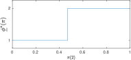
(a) Optimal Policy

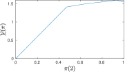
(b) Value Function

Figure 4: Classical Quickest Detection. The optimal policy $\underline{\phi}^{*}(\pi)$ has a threshold structure. So the optimal stopping set $\mathcal{S}=\{\pi:\underline{\phi}^{*}(\pi)=2\}$ is convex. The value function $\underline{\mathcal{V}}(\pi)$ is concave.

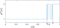
(a) Optimal Policy

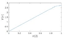
(b) Value Function

Figure 5: Quickest Detection with Multiple Agents. The optimal policy $\phi^{*}(\pi)$ has a multi-threshold structure implying that the optimal stopping set $\mathcal{S}=\{\pi:\phi^{*}(\pi)=2\}$ is not convex (comprises of disconnected regions). The global decision maker exhibits change blindness. As the posterior probability of change $\pi(1)=1-\pi(2)$ increases from $b$ to $a$, the global decision maker declares there is no change in several regions. The value function $\mathcal{V}(\pi)$ is not concave.

V-E Numerical Example. Change Detection of Betting Strategy

Spot fixing is a form of illegal match fixing where players deliberately under-perform in specific segments of a team sport. Identifying spot fixing in cricket and soccer is important with the advent of live betting. Sudden increases in the betting rate, heavy underdog bets and wide swings in the quality of play can prompt monitors to take a closer look at a match. Quickest change detection of these parameters based on monitoring real time betting is relevant for detecting illegal spot-fixing for example in T20 cricket; see also [40, 41, 42]. Here we consider a highly simplified formulation where the aim is detect a sudden change in the intrinsic value (state of nature $x_{n}$) of the bet possibly due to spot fixing.

V-E1 Model

Suppose each anticipatory betting agent $n$ acts according to Sec.II-C and makes decisions ${a}_{n}\in\{{\tt bet},{\overline{\tt bet}}\}$, $\bar{a}_{n}\in[0,W_{0}]$. The agents $n=1,2,\ldots$ act sequentially according to Protocol 1. Each agent $n$ has access to whether the previous agents placed bets, i.e., agent $n$ knows the actions $\{{a}_{l}\in\{{\tt bet},{\overline{\tt bet}}\},l=1,\ldots n-1\}$. The state of nature $x_{n}$ is the underlying value of the bet. Each agent $n$ obtains a noisy value $y_{n}$ of $x_{n}$; this determines its private belief $\eta_{n}$ of $x_{n}$. As in (13), we assume that each agent is risk averse and we choose its risk averse parameter $\beta=\eta_{n}(1)$, i.e., the risk averse parameter of agent $n$ is its belief of the underlying value of the bet. The current score in the game (physical state $s_{n}$) also affects $\beta$; but for simplicity we omit this.

An analyst monitors the betting decisions $\{{a}_{n}\}$. Due to privacy constraints, the amounts bet $\{\bar{a}_{n}\}$ are not known to the analyst. How can the analyst detect a sudden change in the intrinsic value of the bet $x_{n}$ indicating spot fixing?

We chose the anticipatory model parameters $u_{A}=10$, $g=15$, $\iota=0$ (recall notation in (16)). The transition probability $P$ for the jump change and observation probabilities $B$ are as Sec.V-D1. The quickest detection penalties are $d=1$, $f=10$. The system operates according to Protocol 1.

V-E2 Non-concave non-monotone Value Function

Figure 6 displays the quickest detection value function $\mathcal{V}(\pi)$ and optimal policy $\phi^{*}$ (37). Unlike classical quickest detection the value function is non-concave and not increasing, but the optimal policy (not shown) still has a threshold structure. Even this simplistic example shows a rich variation of the value function as $\alpha$ is adjusted: if $\alpha=0.5$, the $\mathcal{V}(\cdot)$ is concave; if $\alpha=1.3$ is non-concave with multiple discontinues in $\mathcal{V}(\cdot)$.

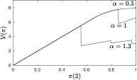
Figure 6: Non-concave value function for quickest change detection in betting strategy of anticipatory agents. The parameters are specified in Sec.V-E.

V-E3 Performance of Quickest Detectors

Figure 7 compares the performance of the quickest detector with anticipatory agents vs the classical quickest detector using the same parameters as above with $\alpha=1$. The observation probability matrix is $B=\begin{bmatrix}\theta&1-\theta\\ 1-\theta&\theta\end{bmatrix}$ where parameter $\theta$ is varied. The delay penalty is fixed at $d=1$ while the false alarm $f\in[0.2,4]$. The optimal expected cost $\mathcal{V}(\cdot)$ is obtained by solving Bellman’s equation (37) by quantizing the beliefs to a grid. We chose $\pi=[0.2,\;0.8]^{\prime}$ in the plot since the value function has a discontinuity just after $\pi(2)=0.8$.

It is interesting to note that for quickest detection with multiple agents, the optimal expected cost remains the same for $\theta\leq 0.92$. Another point to note is that the optimal cost is always larger than classical quickest detection. This is justified in Theorem 4 below via Blackwell dominance.

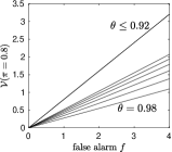
(a) Multi-agent

(b) Classical

Figure 7: Comparison of Optimal Expected Cost for Quickest Detection with Anticipatory Agents vs Classical Quickest Detection

V-F Blackwell Dominance Implications for Optimal Cost

In this section we show that quickest detection with anticipative agents (Protocol 1) results in a cumulative Kolmogorov Shiryaev cost $J_{\phi^{*}}(\pi,s)$ (defined in (31) or equivalently (36)) that is always larger than that of classical quickest detection. In Protocol 1, agents have access to the public belief (which depends on local decisions of previous agents) instead of the actual observations. One expects that this information loss results in less efficient quickest time change detection compared to classical quickest detection. Here we confirm this intuition. The main idea involves Blackwell dominance of observation measures. The result is useful because even though explicit computation of the optimal policy for the setup in Protocol 1 is difficult, we can lower bound the optimal achievable cost by that of classical quickest detection.

First define the optimal policy and cost in classical quickest change detection. Similar to (37), the optimal policy $\underline{\phi}^{*}(\pi)$ and cost $\underline{\mathcal{V}}(\pi)$ incurred in classical quickest detection, satisfy the following stochastic dynamic programming equation:

$$\underline{\phi}^{*}(\pi) =\arg\min_{u\in\mathcal{U}}\underline{Q}(\pi,u),\;\underline{\mathcal{V}}(\pi)=\min_{u\in\mathcal{U}}\underline{Q}(\pi,u),$$ (47)

where $$\underline{Q}(\pi,2)=C(\pi,2)+\sum_{y\in\mathcal{Y}}\underline{\mathcal{V}}\left(T(\pi,y)\right)\sigma(\pi,y),$$

$$\underline{Q}(\pi,1)=C(\pi,1),\qquad\underline{J}_{\mu^{*}}(\pi)=\underline{\mathcal{V}}(\pi).$$

Here $T(\pi,y)$ is the Bayesian filter update defined in (26) and $\underline{J}_{\mu^{*}}(\pi)$ is the cumulative cost of the optimal policy starting with initial belief $\pi$. Note that unlike Protocol 1, in classical quickest detection, there is no public belief update (27) or interaction between the public and private beliefs.

The following theorem says that for any initial belief $\pi$, the optimal detection policy with anticipative agents acting sequentially (Protocol 1) incurs a higher cumulative cost than that of classical quickest detection.

Theorem 4.

Consider the quickest change detection problem involving anticipatory agents described in Protocol 1 and associated value function $\mathcal{V}(\pi,s)$ in (37). Consider also the classical quickest detection problem with value function $\underline{\mathcal{V}}(\pi)$ in (47). Then for any initial belief $\pi\in\Pi$, the optimal cost incurred by classical quickest detection is smaller than that of quickest detection with anticipatory agents. That is, $\underline{\mathcal{V}}(\pi)\leq\mathcal{V}(\pi,s)$ for all $\pi\in\Pi,s\in\mathcal{S}$.

The proof is in the supplementary document.

The intuition behind the proof is as follows. From (29)

$$\begin{split}R^{\pi}_{x,a}(s)&=\int_{\mathcal{Y}}B_{x,y}M^{\pi}_{y,a,s}dy,\\ \text{ where }M^{\pi}_{y,a,s}&\stackrel{{\scriptstyle\text{defn}}}{{=}}I(\mu^{*}_{2,T(\pi,y)}(s,a_{n,1})=a)\end{split}$$ (48)

where $B$ and $M^{\pi}$ are stochastic kernels. Thus observation $y$ with conditional distribution specified by $B$ is said to be more informative than (Blackwell dominates) observation $a$ with conditional distribution $R^{\pi}$, see [36]. The main idea in the proof is that under the assumptions of Theorem 4, the value function $\underline{\mathcal{V}}(\pi)$ is concave for $\pi\in\Pi$. Then the result is established using Jensen’s inequality together with Blackwell dominance on Bellman’s equation (37).

A useful consequence of Theorem 4 is that performance analysis of standard quickest detection [16] applies as a lower bound for quickest detection with anticipatory agents.

VI Discussion

This paper is an early step in addressing sequential detection problems with behavioral economics constraints. Although both signal processing and behavioral economics are mature areas, insights gained by construction of generative anticipatory models, estimation algorithms, along with careful analysis is crucial in designing human-sensor cyber-physical systems.

They main results of the paper are:
1. Formulation of the two stage decision making model of [1] for individual decision makers involving the anticipatory state. The key idea is that the anticipatory state involves the probabilities of future actions thereby leading to time inconsistency in decision making.
2. Characterizing the structure of the subgame Nash equilibrium as a bang-bang controller in the first time stage, and a threshold policy at the second time stage (Theorem 1). The bang-bang structure justifies the observation in [1] that agents with anticipatory emotions may choose to avoid information.
3. Formulation of the multi-agent quickest detection problem where the anticipatory agents interact with a global decision maker. We gave several examples to motivate this problem including change detection in social media accommodation, detecting spot fixing in sports and team-situation awareness.
4. Structural characterization of the unusual structure of the optimal change detection policy (compared to classical quickest detection). Sec.V characterized the structure of the Bayesian belief updates and achievable cost of the quickest detector without brute force computations. We derived important structural properties of the Bayesian updates of the local and global decision makers (Theorem 2 and Theorem 3), constructed a lower bound for the optimal cost incurred using Blackwell dominance (Theorem 4), and presented numerical examples of the unusual structure of the optimal quickest change policy (non-convex stopping region). The multi-threshold change detection policy was interpreted as change blindness, namely people fail to detect surprisingly large changes to scenes.

In future work we will generalize the anticipatory model using the subjective belief multi-horizon formulation of [21]. It is also worthwhile conducting a performance analysis of a multi-threshold detector; see [16] for performance analysis involving a single threshold detector. An important open question is: based on a dataset of actions of an agent, how to identify anticipatory behavior and if so, how to estimate the utility function of an anticipatory agent (inverse reinforcement learning)? For myopic Bayesian utility maximization, [43] give necessary and sufficient conditions for identifying optimal behavior; the utility functions then are feasible points of a set of convex constraints. In [44] we have used such methods to analyze user engagement in massive YouTube datasets.

Supplementary Document

VII Tutorial Example. Social Media based Accommodation Choice

We now discuss an anticipatory decision making example involving choosing accommodation using a social-media based online agency such as Airbnb. The example is a slight generalization of [1] since the rewards are parametrized by a Bayesian posterior $\eta$ (the motivation for this in terms of quickest detection is discussed in the paper).

VII-A Single Anticipatory Agent

Suppose an anticipatory agent chooses between a vacation either at a previous known accommodation $(K)$, or a new accommodation ($N$). The agent has initial wealth of $w_{0}$.

VII-A1 Model

The reviews of accommodation $N$ posted at an online reputation website at times $k=1,2$ are $\text{review}_{k}\in\{G\text{ (good)},B\text{ (bad)}\}$. The physical states $s_{1}$ and $s_{2}$ denote the probability of good review of $N$ at times 1 and 2. For simplicity, assume $s_{2}$ is uniformly distributed in $[0,1]$.

Regarding the actions, at the first stage the agent chooses action $a_{1}\in[0,1]$ which denotes making a non-refundable deposit $2000\,a_{1}$ for booking $K$. At the second stage, the agent makes the final choice of which accommodation to stay in, i.e., $a_{2}\in\,\mathcal{A}_{2}=\{K,N\}$.

Next we model the anticipatory emotions of the agent. Similar to [1], we choose the anticipatory reward to reflect beliefs about pleasure that will be derived in staying respectively at venues $K$ and $N$. We choose the psychological (anticipatory) state $z_{1}$ at time 1 as the conditional probabilities (see (5))

$$\begin{split}z_{1}=\max\{&6000\,p(a_{2}=N,\text{review}_{2}=G|a_{1},\mu_{2}),\\ &4000\,p(a_{2}=K|a_{1},\mu_{2})\}\end{split}$$ (49)

So the anticipatory pleasure increases with the agent’s certainty that an outcome will occur. Also (49) specifies that the anticipatory pleasure is higher for $N$ (since it scaled by 6000) compared to $K$ providing that $\text{review}_{2}$ is good.

We now construct the rewards $r_{1},r_{2}$ defined in (6).

1. Assume each accommodation costs 2000 units.

2. After making a deposit of $2000a_{1}$ for $K$, if $N$ is chosen, then the deposit of $2000a_{1}$ is lost.

3. The benefit accrued by staying in $N$ when rating is $s_{2}$ is $6000s_{2}\eta$; the reward for choosing $K$ is 4000. Here $\eta\in[0,1]$ is the posterior probability that accommodation $N$ is suitable given the most recent review of $N$.

4. Finally, $\beta>0$ denotes the importance of anticipatory reward relative to the reward of the vacation (see (A6)).

Based on the above description, the rewards are

$$\begin{split}&r_{1}=\beta z_{1},\quad\beta>0\\ &r_{\eta,2}(s_{2},a_{2}=N,a_{1})=6000s_{2}\eta+w_{0}-2000(1+a_{1}),\\ &r_{\eta,2}(s_{2},a_{2}=K,a_{1})=4000+w_{0}-2000\end{split}$$

VII-A2 Structural Result for Nash equilibrium

For the above example, we can verify Assumptions (A1)-(A7) hold and therefore Theorem 1 holds. Specifically, (A1) holds by formulation; (A2) holds trivially since $r_{\eta,2}$ is linear in $a_{1}$; (A3) holds since $r_{\eta,2}(s_{2},a_{2}=K,a_{1})$ is independent of $s_{2}$; (A4) and (A5) hold trivially since $\Delta_{\eta}$ is linear in $s_{2}$ and $a_{1}$; (A6) holds by construction since it is easily shown that for optimal policy $\mu_{2}^{*}$, $z_{1}=4000\,p(a_{2}=K|a_{1},\mu_{2}^{*})$. Finally, (A7) holds since $p(s_{2})$ is the uniform density.

Therefore from Theorem 1 it follows that $\mu_{2}^{*}$ has a threshold structure (20), and $\mu_{1}^{*}$ has a bang-bang structure (21).

Therefore the interpretation of deliberate avoidance of information discussed below Theorem 1 holds. Specifically, due to the bang-bang structure of (21), the agent makes a full deposit $a_{1}=1$ if $\beta>\beta^{*}$ for the accommodation $K$. Yet this full non-refundable deposit does not guarantee that the agent will choose $a_{2}=K$ since if $s_{2}>s_{2}^{*}(a_{1})$, then the agent will choose $a_{2}=N$. Thus the agent might deliberately choose not to observe the state $s_{2}$ in order not to lose the deposit paid at time 1 to secure $K$.

VII-A3 Explicit Evaluation of Nash equilibrium

Given the simple structure above, we can go beyond Theorem 1 and solve explicitly for the subgame Nash equilibrium specified by (8), (10). The computations below are similar to [1].

From the extended Bellman equation (8), $\mu_{2}^{*}(s_{2},a_{1})$ has threshold structure

$$\mu_{2,\eta}^{*}(s_{2},a_{1})=\operatornamewithlimits{argmax}_{a_{2}}r_{\eta,2}(s_{2},a_{2},a_{1})=\begin{cases}N&\text{ if }s_{2}\geq\frac{2+a_{1}}{3\eta}\\ K&s_{2}<\frac{2+a_{1}}{3\eta}\end{cases}$$ (50)

with associated value function

$$V_{2}(s_{2},\mu_{2}^{*})=\max_{a_{2}}\{r_{\eta,2}(s_{2},a_{2},a_{1})\}\\ =\begin{cases}6000s_{2}\eta+w_{0}-2000(1+a_{1})&s_{2}\geq\frac{2+a_{1}}{3\eta}\\ 4000+w_{0}-2000&s_{2}<\frac{2+a_{1}}{3\eta}\end{cases}$$

In order to determine the policy $\mu_{1}^{*}$ and value function $V_{1}$, let us first compute the psychological state $z_{1}$ in (49) under $\mu_{2}^{*}$. Since $s_{2}$ is uniformly distributed in $[0,1]$, clearly

$$\begin{split}p(a_{2}&=K|a_{1},\mu_{2}^{*})=\mathbb{P}(\{s_{2}:\mu_{2}^{*}(s_{2})=K\}|a_{1})\\ &=\int_{\mathcal{S}}p(s_{2}|s_{1})I(s_{2}:\mu_{2}^{*}(s_{2}=K))\,ds_{2}\\ &=\int_{\mathcal{S}}p(s_{2})\,I(s_{2}\in[0,\frac{2+a_{1}}{3\eta}])ds_{2}\\ &=\min\{\frac{2+a_{1}}{3\eta},1\}\end{split}$$ (51)

$$\begin{split}&p(a_{2}=N,\text{review}_{2}=G|s_{2},a_{1},\mu_{2}^{*})\\ &=p(\text{review}_{2}=G)p(a_{2}=N|a_{1},s_{2},\mu_{2}^{*})=s_{2}\,I(s_{2}\in[\frac{2+a_{1}}{3\eta},1])\\ \end{split}$$

Therefore,

$$\begin{split}&p(a_{2}=N,\text{review}_{2}=G\,|a_{1},\mu_{2}^{*})\\ &=\int_{\mathcal{S}}s_{2}\,I(s_{2}\in[\frac{2+a_{1}}{3\eta},1])p(s_{2})ds_{2}=\max\{\int_{\frac{2+a_{1}}{3\eta}}^{1}s_{2}ds_{2},0\}\\ &=\max\{\frac{9\eta^{2}-4-4a_{1}-a_{1}^{2}}{18\,\eta^{2}},0\}\end{split}$$ (52)

Then using notation (9) and (49), the psychological state is

$$z_{1}=\max\{4000\,p(a_{2}=K|a_{1},\mu_{2}^{*}),\\ 6000p(a_{2}=N,\text{review}_{2}=G\,|a_{1},\mu_{2}^{*})\}\\ =4000\,p(a_{2}=K|a_{1},\mu_{2}^{*})$$ (53)

The last equality is verified since comparing the two terms involves a scalar quadratic inequality in $\eta\in[0,1]$.

Then substituting $V_{2}$ computed in (50) into (10) yields

$$V_{1}(s_{1})=\max_{a_{1}\in\,\mathcal{A}_{1}}\{\beta z_{1}+\int_{0}^{1}V_{2}(s_{2})ds_{2}\}$$

It is easily verified that the expression within $\{\cdot\}$ is convex in $a_{1}$. Since $\,\mathcal{A}_{1}=[0,1]$ is convex, the maximum is achieved at an extreme point $a_{1}=0$ or $a_{1}=1$. Thus the optimal policy $\mu_{1}^{*}$ at time 1 is a $(\beta,\eta)$ dependent bang-bang policy:

$$\mu_{1,\eta}^{*}=\begin{cases}1\text{ (full deposit) }&\text{ if }\beta>1-3\eta+\frac{9\eta^{2}}{4}\\ 0\text{ (no deposit) }&\text{ if }\beta\leq 1-3\eta+\frac{9\eta^{2}}{4}\end{cases}$$ (54)

Recall $\eta$ is a Bayesian parameter (see footnote 9) that is defined as the private belief in Sec.IV in the context of quickest detection, and $\beta>0$ is a scaling constant (A6).

VII-B Quickest Change Detection

Here we comment on how the above example extends to social media based decision making such as media based accommodation systems. Individual anticipatory agents make local decisions sequentially whether to rent a property; these decisions are affected by the reviews (decisions) of previous agents. The global decision maker (e.g. Airbnb) monitors these local decisions. How can the global decision maker detect if there is a sudden change in the demand for a specific accommodation due to the presence of a new competitor? Alternatively, how can the global decision maker detect a sudden change in the quality of an accommodation?

1. The underlying state of nature $x_{n}$ is the intrinsic value of the accommodation $K$; i.e., the ground truth. The value of $x_{n}$ depends on the cost of $K$ and cost of competitors.

2. $y_{n}$ is an extrinsic measurement made by the agent regarding $x_{n}$. $y_{n}$ is an interpretation of a competitor, a recent photo/review comparing $K$ with a competitor, etc.

3. $\pi_{n-1}$: This is the histogram available to the agent from the rating site comparing $K$ with a competitor and so is reflective of $p(x_{n-1}|a_{1},\ldots,a_{n-1})$.

4. Recall $s_{n}$ denotes the probability of good reviews of $N$. As discussed in the main paper, by allowing the transition kernel of $s_{n}$ to depend on the ground truth $x_{n}$, we allow for the reviews to change with changing ground truth.

5. The agent updates its belief $\eta_{n}$ based on this information. The Bayesian update is a useful idealization of the agent’s behavior; see Theorem 2 below.

6. The agent then makes decisions $a_{n,1},a_{n,2}$ according to Protocol 1.

Given the sequence of decisions $\{a_{n}\}$, the global decision maker (e.g. Airbnb) wishes to detect if there is a sudden appearance of competition or sudden change in quality of the accommodation.

VIII Human-Sensor System

Quickest change detection involves decision making in a partially observed Bayesian setting. In the context of this paper, there are two interpretations.

1. In human-sensor interface systems, each anticipatory agent is equipped with a sensing/computing device. The sensing device observes the state of nature (Markov chain) in noise. The computing device evaluates the posterior and provides the agent with these probabilities. The agent (human) then makes anticipatory decisions $a_{1},a_{2}$ as detailed in Sec.III.

2. The second interpretation is as follows: If the anticipative agent $n$ makes recommendations that are monotone and ordinal in the observations and monotone in the prior, then they mimic the Bayesian social learning model. Even if the agent does not exactly follow a Bayesian social learning model, its monotone ordinal behavior implies that such a Bayesian model is a useful idealization. Humans typically make monotone decisions - the more favorable the private observation, the higher the recommendation. Humans make ordinal decisions.

IX Proofs of Theorems

IX-A Proof of Theorem 1

Remark. Relaxing Assumption (A4). Instead of (A4), the following weaker condition based on the classic implicit function theorem [34] can be used. Assume (i) $\Delta_{\eta}(s_{2},a_{1})$ has continuous first partial derivatives; (ii) $\Delta_{\eta}(s_{2}^{*},a_{1})=0\implies\partial\Delta_{\eta}(s_{2}^{*},a_{1})/\partial s_{2}\neq 0$. Then by the implicit function theorem, the solution $s_{2}^{*}(a_{1})$ is continuously differentiable on an open subset of $(0,1)$. Assume that this subset is convex.

Proof.

For convenience we omit parameter $\eta$ in the notation.

Statement 1. By (A3), $r_{\eta,2}$ is supermodular in $(s_{2},a_{2})$. Thus by Topkis theorem [32], $\mu_{2}^{*}(s_{2},a_{1})$ is non-decreasing in $s_{2}$ for fixed $a_{1}$. So either $\mu_{2}^{*}(s_{2},a_{1})$ is constant wrt $s_{2}$ (in which case the theorem holds trivially); or for each $a_{1}$ there exists an indifference state $s_{2}^{*}\in[0,1]$ such that $\mu_{2}^{*}(s_{2},a_{1})$ switches from 1 to 2 as $s_{2}$ increases. Clearly the indifference set $\{s_{2},a_{1}:\Delta_{\eta}(s_{2},a_{1})=0\}$ determines where $\mu_{2}^{*}(s_{2},a_{1})$ switches from 1 to 2. By (A4), a solution $s_{2}^{*}(a_{1})$ exists to $\Delta_{\eta}(s_{2},a_{1})=0$ for $a_{1}\in(0,1)$. Hence, $\mu_{2}^{*}$ has the threshold structure (20).

Statement 2. Proving statement 2, is equivalent to showing convexity in $a_{1}$ of the solution $s_{2}^{*}(a_{1})$ of the algebraic equation $\Delta_{\eta}(s_{2},a_{1})=0$. By (A4), $s_{2}^{*}(a_{1})$ is continuously differentiable in $a_{1}$. It is verified by elementary calculus that

$$\frac{\partial^{2}s_{2}^{*}}{\partial a_{1}^{2}}=\frac{1}{(\partial\Delta_{\eta}/\partial s_{2})^{2}}\,\big{[}\frac{\partial\Delta_{\eta}}{\partial a_{1}}\frac{\partial^{2}\Delta_{\eta}}{\partial s_{2}a_{1}}-\frac{\partial\Delta_{\eta}}{\partial s_{2}}\frac{\partial^{2}\Delta_{\eta}}{\partial a_{1}^{2}}\big{]}$$

So $s_{2}^{*}(a_{1})$ is convex in $a_{1}$ iff (A5) holds; see [33] for a more general multidimensional result.

Statement 3(a). From (A6), the psychological state is

$$\begin{split}&z_{1}=\max_{a\in\,\mathcal{A}_{2}}\{\int_{\mathcal{S}}I(s_{2}:\mu_{2}^{*}(s_{2},a_{1})=a)\,\Psi(a,s_{2})\,p(s_{2}|s_{1})\,ds_{2}\}\\ &\quad=\max\{\int_{0}^{s_{2}^{*}(a_{1})}\Psi(1,s_{2})\,p(s_{2}|s_{1})\,ds_{2},\\ &\qquad\qquad\qquad\int_{s_{2}^{*}(a_{1})}^{1}\Psi(2,s_{2})\,p(s_{2}|s_{1})\,ds_{2}\}\\ &\quad=\max\big{\{}F_{1}(s_{2}^{*}(a_{1}))-F_{1}(0),F_{2}(1)-F_{2}(s_{2}^{*}(a_{1}))\big{\}}\\ &\text{ where }F_{a}(y)=\int_{0}^{y}\Psi(a,s_{2})\,p(s_{2}|s_{1})\,ds_{2}\end{split}$$

By (A7), $F_{1}(y)$ and $-F_{2}(y)$ are increasing convex functions of $y$. Since $s_{2}^{*}(a_{1})$ is convex in $a_{1}$ (by Statement 2), the composition functions $F_{1}(s_{2}^{*}(a_{1}))$ and $-F_{2}(s_{2}^{*}(a_{1}))$ are convex. Thus $r_{1}=\beta z_{1}$ being the max of two convex functions is convex in $a_{1}$. This together with (A2) implies that the reward-to-go $J_{1}(s_{1},a_{1},\mu_{2}^{*})$ is convex in $a_{1}$.

Statement 3(b). Finally a convex function on a convex set (recall $a_{1}\in\,\mathcal{A}_{1}=[0,1]$) achieves its global maximum at an extreme point [45, Theorem 3, pp.181]. Hence the bang-bang structure (21) holds for $\mu_{1}^{*}$. ∎

IX-B Proof of Theorem 2

Proof.

The proof uses MLR stochastic dominance (defined in footnote 7) and the following single crossing condition:

Definition (Single Crossing [46]).

$g:\mathbf{Y}\times\mathbb{A}\rightarrow{\rm IR}$ satisfies a single crossing condition in $(y,a)$ if $g(y,a)-g(y,\bar{a})\geq 0$ implies $g(\bar{y},a)-g(\bar{y},\bar{a})\geq 0$ for $\bar{a}>a$ and $\bar{y}>y$. Then $a^{*}(y)=\operatornamewithlimits{argmin}_{a}g(y,a)$ is increasing in $y$. ∎

By (A6) it follows that [36] the Bayesian update satisfies

$$\frac{B_{y}P^{\prime}\pi}{\mathbf{1}^{\prime}B_{y}P^{\prime}\pi}\leq_{r}\frac{B_{\bar{y}}P^{\prime}\pi}{\mathbf{1}^{\prime}B_{\bar{y}}P^{\prime}\pi},\quad\bar{y}>y$$

where $\leq_{r}$ is the MLR stochastic order. (Indeed, the MLR order is closed under conditional expectation.) By supermodularity (A7) $r_{a+1}-r_{a}$ is a vector with increasing elements. Therefore

$$(r_{a+1}-r_{a})^{\prime}\frac{B_{y}P^{\prime}\pi}{\mathbf{1}^{\prime}B_{y}P^{\prime}\pi}\leq(r_{a+1}-r_{a})^{\prime}\frac{B_{\bar{y}}P^{\prime}\pi}{\mathbf{1}^{\prime}B_{\bar{y}}\pi}$$

Since the denominator is non-negative, it follows that $(r_{a+1}-r_{a})^{\prime}B_{\bar{y}}\pi\leq 0\implies(r_{a+1}-r_{a})^{\prime}B_{y}\pi\leq 0$. This implies that $r_{a}^{\prime}B_{y}\pi$ satisfies a single crossing condition in $(y,a)$. Therefore $a_{n}(\pi,y)=\operatornamewithlimits{argmax}_{a}r_{a}^{\prime}B_{y}\pi$ is increasing in $y$ for any belief $\pi$. ∎

IX-C Proof of Theorem 3

Proof.

The single crossing property (40) implies

$$\{\pi:(r_{1}-r_{2})^{\prime}B_{y}P^{\prime}\pi\leq 0\}\subseteq\{\pi:(r_{1}-r_{2})^{\prime}B_{\bar{y}}P^{\prime}\pi\leq 0\}$$

for $y<\bar{y}$. This implies (41). From (29) we can write

$$\begin{split}R^{\pi}_{x,a}(s)&=\sum_{\mathcal{Y}}B_{x,y}M^{\pi}_{y,a,s},\\ \text{ where }M^{\pi}_{y,a,s}&\stackrel{{\scriptstyle\text{defn}}}{{=}}I(\mu^{*}_{2,T(\pi,y)}(s,a_{n,1})=a)\end{split}$$ (55)

where $B$ and $M^{\pi}$ are stochastic matrices. This yields (43).

∎

IX-D Proof of Theorem 4

Proof.

It is well known [36] (and straightforwardly demonstrated by induction) that the value function $\underline{V}_{k}(\pi)$ for classical quickest detection is concave over $\Pi$ for any $k$. We then use the Blackwell dominance condition (55). The public belief update (27) can be expressed in terms of the private belief update (26) as

$$\bar{T}(\pi,a,s)=\sum_{y\in\mathcal{Y}}T(\pi,y)\frac{\sigma(\pi,y)}{\bar{\sigma}(\pi,a,s)}\,M^{\pi}_{y,a,s}\\ \text{ and }\bar{\sigma}(\pi,a,s)=\sum_{y\in\mathcal{Y}}\sigma(\pi,y)M^{\pi}_{y,a,s}$$ (56)

Note that $\frac{\sigma(\pi,y)}{\bar{\sigma}(\pi,a,s)}M^{\pi}_{y,a,s}$ is a probability measure wrt $y$. Since $\underline{\mathcal{V}}_{k}(\cdot)$ is concave for $\pi\in\Pi$, using Jensen’s inequality it follows that

$$\underline{\mathcal{V}}_{k}(\bar{T}(\pi,a,s)) =\underline{\mathcal{V}}_{k}\left(\sum_{y\in\mathcal{Y}}T(\pi,y)\frac{\sigma(\pi,y)}{\bar{\sigma}(\pi,a,s)}M^{\pi}_{y,a,s}\right)$$

$$\geq\sum_{y\in\mathcal{Y}}\underline{\mathcal{V}}_{k}(T(\pi,y))\frac{\sigma(\pi,y)}{\bar{\sigma}(\pi,a,s)}M^{\pi}_{y,a,s}$$

Therefore for each $\bar{s}\in\mathcal{S}$,

$$\sum_{a}\underline{\mathcal{V}}_{k}(\bar{T}(\pi,a,\bar{s}))\,\bar{\sigma}(\pi,a,\bar{s})\geq\sum_{y}\underline{\mathcal{V}}_{k}(T(\pi,y))\,\sigma(\pi,y).$$

Therefore multiplying by $p(\bar{s}|s)$ and integrating we have

$$\int_{\mathcal{S}}\sum_{a}\underline{V}_{k}(\bar{T}(\pi,a,\bar{s}))\,\bar{\sigma}(\pi,a,\bar{s})p(\bar{s}|s)\,d\bar{s}\\ \geq\sum_{y}\underline{V}_{k}(T(\pi,y))\,\sigma(\pi,y).$$ (57)

The proof of Theorem 4 then follows by mathematical induction using the value iteration algorithm (39). Assume $\mathcal{V}_{k}(\pi,s)\geq\underline{\mathcal{V}}_{k}(\pi)$ for $\pi\in\Pi$. Then

$$C(\pi,2)+\int_{\mathcal{S}}\sum_{a}\mathcal{V}_{k}(\bar{T}(\pi,a,\bar{s}),\bar{s})\bar{\sigma}(\pi,a,\bar{s})\,p(\bar{s}|s)d\bar{s}$$

$$\geq C(\pi,2)+\int_{\mathcal{S}}\sum_{a}\underline{\mathcal{V}}_{k}(\bar{T}(\pi,a,\bar{s}))\,\bar{\sigma}(\pi,a,\bar{s})\,p(\bar{s}|s)d\bar{s}$$

$$\geq C(\pi,2)+\sum_{y}\underline{\mathcal{V}}_{k}(T(\pi,y))\,\sigma(\pi,y)$$

where the second inequality follows from (57). Thus $\mathcal{V}_{k+1}(\pi,s)\geq\underline{\mathcal{V}}_{k+1}(\pi)$. This completes the induction step. Since value iteration converges pointwise, $\mathcal{V}(\pi,s)\geq\underline{\mathcal{V}}(\pi)$ thus proving the theorem.

∎

References

- [1] A. Caplin and J. Leahy, “Psychological expected utility theory and anticipatory feelings,” The Quarterly Journal of Economics, vol. 116, no. 1, pp. 55–79, 2001.
- [2] R. Rosen, “Anticipatory systems,” in Anticipatory systems. Springer, 2012, pp. 313–370.
- [3] A. N. Shiryaev, “On optimum methods in quickest detection problems,” Theory of Probability and its Applications, vol. 8, no. 1, pp. 22–46, 1963.
- [4] R. Bénabou and J. Tirole, “Mindful economics: The production, consumption, and value of beliefs,” Journal of Economic Perspectives, vol. 30, no. 3, pp. 141–64, 2016.
- [5] C. J. Charpentier, E. S. Bromberg-Martin, and T. Sharot, “Valuation of knowledge and ignorance in mesolimbic reward circuitry,” Proceedings of the National Academy of Sciences, vol. 115, no. 31, pp. E7255–E7264, 2018.
- [6] J. O. Cook and L. W. Barnes Jr, “Choice of delay of inevitable shock.” Journal of Abnormal and Social Psychology, vol. 68, no. 6, p. 669, 1964.
- [7] S. M. Miller and C. E. Mangan, “Interacting effects of information and coping style in adapting to gynecologic stress: should the doctor tell all?” Journal of personality and social psychology, vol. 45, no. 1, p. 223, 1983.
- [8] M. R. Endsley, Designing for situation awareness: An approach to user-centered design. CRC press, 2016.
- [9] E. Blasch, “Enhanced air operations using jview for an air-ground fused situation awareness UDOP,” in 2013 IEEE/AIAA 32nd Digital Avionics Systems Conference (DASC). IEEE, 2013, pp. 5A5–1.
- [10] G. Klein, D. Snowden, and C. L. Pin, “Anticipatory thinking,” Informed by knowledge: Expert performance in complex situations, pp. 235–245, 2011.
- [11] Z. Lanir, “Fundamental surprise,” Eugene, OR: Decision Research, 1986.
- [12] T. Björk and A. Murgoci, “A theory of Markovian time-inconsistent stochastic control in discrete time,” Finance and Stochastics, vol. 18, no. 3, pp. 545–592, 2014.
- [13] D. Kahneman and A. Tversky, “Prospect theory: An analysis of decision under risk,” Econometrica, pp. 263–291, 1979.
- [14] M. K. Brunnermeier and J. A. Parker, “Optimal expectations,” The American Economic Review, vol. 95, no. 4, pp. 1092–1118, 2005.
- [15] H. V. Poor and O. Hadjiliadis, Quickest Detection. Cambridge University Press, 2008.
- [16] A. G. Tartakovsky and V. V. Veeravalli, “General asymptotic Bayesian theory of quickest change detection,” Theory of Probability and its Applications, vol. 49, no. 3, pp. 458–497, 2005.
- [17] J. C. Gorman, N. J. Cooke, and J. L. Winner, “Measuring team situation awareness in decentralized command and control environments,” Ergonomics, vol. 49, no. 12-13, pp. 1312–1325, 2006.
- [18] T. Erlandsson, T. Helldin, G. Falkman, and L. Niklasson, “Information fusion supporting team situation awareness for future fighting aircraft,” in 2010 13th International Conference on Information Fusion. IEEE, 2010, pp. 1–8.
- [19] B. L. Hooey, B. F. Gore, C. D. Wickens, S. Scott-Nash, C. Socash, E. Salud, and D. C. Foyle, “Modeling pilot situation awareness,” in Human modelling in assisted transportation. Springer, 2011, pp. 207–213.
- [20] J. Boger, P. Poupart, and J. Hoey, “A decision-theoretic approach to task assistance for persons with dementia,” in Proceedings of the International Joint Conference on Artificial Intelligence, 2005, pp. 1293–1299.
- [21] M. K. Brunnermeier, F. Papakonstantinou, and J. A. Parker, “Optimal time-inconsistent beliefs: Misplanning, procrastination, and commitment,” Management Science, vol. 63, no. 5, pp. 1318–1340, 2017.
- [22] C. Chamley, Rational herds: Economic Models of Social Learning. Cambridge University Press, 2004.
- [23] V. Krishnamurthy, “Quickest detection POMDPs with social learning: Interaction of local and global decision makers,” IEEE Transactions on Information Theory, vol. 58, no. 8, pp. 5563–5587, 2012.
- [24] V. Krishnamurthy and H. V. Poor, “A tutorial on interactive sensing in social networks,” IEEE Transactions on Computational Social Systems, vol. 1, no. 1, pp. 3–21, March 2014.
- [25] V. Bordignon, V. Matta, and A. H. Sayed, “Adaptive social learning,” arXiv preprint arXiv:2004.02494, 2020.
- [26] J. Tsitsiklis, “Decentralized detection,” Advances in Statistical Signal Processing, vol. 2, pp. 297–344, 1993.
- [27] R. Viswanathan and P. Varshney, “Distributed detection with multiple sensors I. Fundamentals,” Proceedings of the IEEE, vol. 85, no. 1, pp. 54–63, 1997.
- [28] D. J. Simons and R. A. Rensink, “Change blindness: Past, present, and future,” Trends in cognitive sciences, vol. 9, no. 1, pp. 16–20, 2005.
- [29] D. M. Kreps and E. L. Porteus, “Temporal resolution of uncertainty and dynamic choice theory,” Econometrica: journal of the Econometric Society, pp. 185–200, 1978.
- [30] G. F. Loewenstein, E. U. Weber, C. K. Hsee, and N. Welch, “Risk as feelings.” Psychological bulletin, vol. 127, no. 2, p. 267, 2001.
- [31] P. A. Samuelson, “Probability, utility, and the independence axiom,” Econometrica: Journal of the Econometric Society, pp. 670–678, 1952.
- [32] D. M. Topkis, Supermodularity and Complementarity. Princeton University Press, 1998.
- [33] W. A. Brock and R. G. Thompson, “Convex solutions of implicit relations,” Mathematics Magazine, vol. 39, no. 4, pp. 208–211, 1966.
- [34] T. M. Apostol, “Mathematical analysis,” 1974.
- [35] M. Avellaneda and S. Stoikov, “High-frequency trading in a limit order book,” Quantitative Finance, vol. 8, no. 3, pp. 217–224, Apr 2008.
- [36] V. Krishnamurthy, Partially Observed Markov Decision Processes. From Filtering to Controlled Sensing. Cambridge University Press, 2016.
- [37] O. Hernández-Lerma and J. B. Laserre, Discrete-Time Markov Control Processes: Basic Optimality Criteria. New York: Springer-Verlag, 1996.
- [38] S. Karlin and Y. Rinott, “Classes of orderings of measures and related correlation inequalities. I. Multivariate totally positive distributions,” Journal of Multivariate Analysis, vol. 10, no. 4, pp. 467–498, December 1980.
- [39] P. Milgrom, “Good news and bad news: Representation theorems and applications,” Bell Journal of Economics, vol. 12, no. 2, pp. 380–391, 1981.
- [40] B. Abarbanel and M. R. Johnson, “Esports consumer perspectives on match-fixing: implications for gambling awareness and game integrity,” International Gambling Studies, vol. 19, no. 2, pp. 296–311, 2019.
- [41] D. Forrest and I. G. McHale, “Using statistics to detect match fixing in sport,” IMA Journal of Management Mathematics, vol. 30, no. 4, pp. 431–449, 2019.
- [42] H. Qureshi and A. Verma, “It is just not cricket,” in Match-Fixing in International Sports. Springer, 2013, pp. 69–88.
- [43] A. Caplin and M. Dean, “Revealed preference, rational inattention, and costly information acquisition,” The American Economic Review, vol. 105, no. 7, pp. 2183–2203, 2015.
- [44] W. Hoiles, V. Krishnamurthy, and K. Pattanayak, “Rationally inattentive inverse reinforcement learning explains youtube commenting behavior,” Journal of Machine Learning Research, vol. 21, no. 170, pp. 1–39, 2020.
- [45] D. Luenberger, Linear and Nonlinear Programming, Second ed. Addison Wesley, 1984.
- [46] R. Amir, “Supermodularity and complementarity in economics: An elementary survey,” Southern Economic Journal, vol. 71, no. 3, pp. 636–660, 2005.