Vortices with magnetic field inversion in noncentrosymmetric superconductors

Abstract

Superconducting materials with noncentrosymmetric lattices lacking space inversion symmetry exhibit a variety of interesting parity-breaking phenomena, including the magneto-electric effect, spin-polarized currents, helical states, and the unusual Josephson effect. We demonstrate, within a Ginzburg-Landau framework describing noncentrosymmetric superconductors with $O$ point group symmetry, that vortices can exhibit an inversion of the magnetic field at a certain distance from the vortex core. In stark contrast to conventional superconducting vortices, the magnetic-field reversal in the parity-broken superconductor leads to non-monotonic intervortex forces, and, as a consequence, to the exotic properties of the vortex matter such as the formation of vortex bound states, vortex clusters, and the appearance of metastable vortex/anti-vortex bound states.

I Introduction

noncentrosymmetric superconductors are superconducting materials whose crystal structure is not symmetric under the spatial inversion. These parity-breaking materials have attracted much theoretical Bulaevskii et al. (1976); Levitov et al. (1985); Mineev and Samokhin (1994); Edelstein (1996); Agterberg (2003); Samokhin (2004) and experimental Bauer et al. (2004); Samokhin et al. (2004); Yuan et al. (2006); Cameron et al. (2019); Khasanov et al. (2020) interest, as they make it possible to investigate spontaneous breaking of a continuous symmetry in a parity-violating medium (for recent reviews, see Bauer and Sigrist (2012); Yip (2014); Smidman et al. (2017)). The parity-breaking nature of the superconducting order parameter Samokhin et al. (2004); Yuan et al. (2006) in noncentrosymmetric superconductors leads to various unusual magneto-electric phenomena due to the mixing of singlet and triplet components of the superconducting condensate, correlations between supercurrents and spin polarization, to the existence of helical states, and to unusual structure of vortex lattices.

Moreover, parity breaking in noncentrosymmetric superconductors also results in an unconventional Josephson effect, where the junction features a phase-shifted relation for the Josephson current Buzdin (2008); Konschelle and Buzdin (2009). Unconventional Josephson junctions consisting of two noncentrosymmetric superconductors linked by a uniaxial ferromagnet were recently proposed as the element of a qubit that avoids the use of an offset magnetic flux, enabling a simpler and more robust architecture Chernodub et al. (2019).

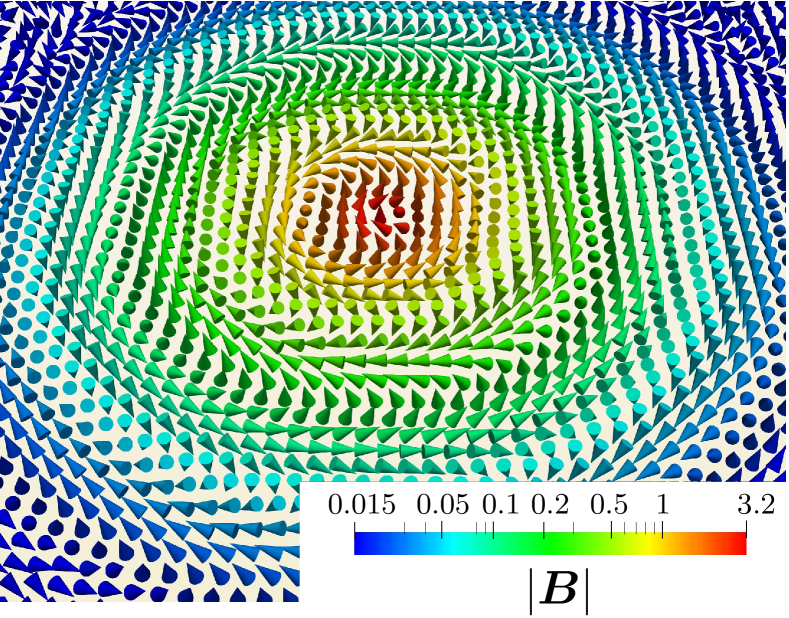
Figure 1: Inversion patterns of the magnetic field ${\boldsymbol{B}}$ of a vortex in a noncentrosymmetric superconductor. The magnetic field forms helicoidal patterns around a straight static vortex. As the distance from the vortex core increases, the longitudinal (parallel to the vortex core) component of the magnetic field may change its sign. The magnetic field may exhibit several sign reversals in the normal plane. In the picture, which is a result of a numerical simulation of the Ginzburg-Landau theory, the colors encode the amplitude of the magnetic field ${\boldsymbol{B}}$, in a normal plane with respect to the vortex line while the arrows show the orientation of the field.

In the macroscopic description of such superconducting states, the lack of inversion symmetry yields new terms in the Ginzburg-Landau free energy termed ‘Lifshitz invariants’. These terms directly couple the magnetic field with an electric current and thus lead to a variety of new effects that are absent in conventional superconductors. The explicit form of the allowed Lifshitz invariant depends on the point symmetry group of the underlying crystal structure.

In this paper, we consider a particular class of noncentrosymmetric superconductors that break the discrete group of parity reversals and, at the same time, are invariant under spatial rotations. The corresponding Lifshitz invariant featuring these symmetries is described by the simple, parity-violating isotropic term, $\propto\mathrm{Im}(\psi^{*}{\boldsymbol{D}}\psi)\cdot{\boldsymbol{B}}$. This particular structure describes noncentrosymmetric superconductors with $O$ point group symmetry such as Li₂Pt₃B Badica et al. (2005); Yuan et al. (2006), Mo₃Al₂C Karki et al. (2010); Bauer et al. (2010), and PtSbS Mizutani et al. (2019).

Vortex states in cubic noncentrosymmetric superconductors feature a transverse magnetic field, in addition to the ordinary longitudinal field. Consequently, they also carry a longitudinal current on top of the usual transverse screening currents Lu and Yip (2008a, b); Kashyap and Agterberg (2013). Therefore, as illustrated in Fig. 1, both the superconducting current and the magnetic field form a helical-like structure that winds around the vortex core (for additional material illustrating the helical spatial structure of the magnetic streamlines, see Appendix B, and supplemental animations [SeeSupplementalvideomaterial:][]Supplemental-arxiv described in Appendix C). Previous theoretical papers studied vortices in the perturbative regime where the coupling to the Lifshitz invariant is small, either in the London limit (with a large Ginzburg-Landau parameter) Lu and Yip (2008a, b), or beyond it Kashyap and Agterberg (2013). For currently known noncentrosymmetric materials, these approximations are valid since the magnitude of the Lifshitz invariants, which can be estimated in a weak-coupling approximation, is typically small. We propose here a general study of vortices, for all possible values of the Lifshitz invariant coupling, both in the London limit and beyond.

We demonstrate that vortices may feature an inversion of the magnetic field at a distance of about 4$\lambda_{L}$ from the vortex center. Moreover, for rather high values of the coupling $\gamma$, alternating reversals may occur several times, at different distances from the vortex core. Such an inversion of the magnetic field is illustrated, in Fig. 1. The reversal of the magnetic field, which is in stark contrast to conventional superconducting vortices, becomes increasingly important for larger couplings of the Lifshitz invariant term. This property of field inversion is responsible for other unusual behaviors, also absent in conventional type-2 superconductors. Indeed, we show that it leads to the formation of vortex bound states, vortex clusters, and meta-stable pairs of vortex and anti-vortex. These phenomena should have numerous physical consequences on the response of noncentrosymmetric superconductors to an external magnetic field.

The paper is organized as follows. In Sec. II, we introduce the phenomenological Ginzburg-Landau theory that describes the superconducting state of a noncentrosymmetric material with $O$ point group symmetry. Next, in Sec. III we investigate the properties of single vortices both in the London limit and beyond it. We also demonstrate that the parity-breaking superconductors can feature an inversion of the longitudinal magnetic field. This observation suggests that the intervortex interaction in parity-odd superconductors might be much richer than that for a conventional superconductor. Hence we derive analytically the intervortex interaction energy in the London limit in Sec. IV. We show that the interaction potential depends non-monotonically on the intervortex distance, which leads to the existence of vortex bound states. Using numerical minimization of the Ginzburg-Landau free energy, we further observe that such bound states persist beyond the London limit. Our conclusions and discussion of further prospects are given in the last section.

II Theoretical framework

We consider noncentrosymmetric superconductors with the crystal structure possessing the $O$ point group symmetry. Such materials are described by the Ginzburg-Landau free energy $F=\int d^{3}x\,\mathcal{F}$ with the free-energy density given by (see e.g. Bauer and Sigrist (2012); Agterberg (2012)):

$$\mathcal{F}=\frac{{\boldsymbol{B}}^{2}}{8\pi}+k|{\boldsymbol{D}}\psi|^{2}+\gamma{\boldsymbol{j}}\cdot{\boldsymbol{B}}+\frac{\beta}{2}(|\psi|^{2}-\psi_{0}^{2})^{2}\,,$$ (1)

where ${\boldsymbol{j}}=2e\,\mathrm{Im}\left(\psi^{*}{\boldsymbol{D}}\psi\right)$; we use $\hbar{=}c{=}1$. Here, the single component order parameter $\psi=|\psi|\text{e}^{i\varphi}$ is a complex scalar field that is coupled to the vector potential ${\boldsymbol{A}}$ of the magnetic field ${\boldsymbol{B}}={\boldsymbol{\nabla}}\!\times\!{\boldsymbol{A}}$ through the gauge derivative ${\boldsymbol{D}}\equiv{\boldsymbol{\nabla}}-ie{\boldsymbol{A}}$, where $e$ is a gauge coupling. The explicit breaking of the inversion symmetry is accounted for by the Lifshitz invariant term with the prefactor $\gamma$, which directly couples the magnetic field ${\boldsymbol{B}}$ and ${\boldsymbol{j}}=2e|\psi|^{2}({\boldsymbol{\nabla}}\varphi-e{\boldsymbol{A}})$. In the absence of parity breaking, when $\gamma=0$, the vector ${\boldsymbol{j}}$ matches the usual superconducting current. The parameter $\gamma$, which controls the strength of the parity breaking, can be chosen to be positive without loss of generality. The other coupling constants $k$ and $\beta$ describe, respectively, the magnitude of the kinetic and potential terms in the free energy (1).

The variation of the free energy (1) with respect to the scalar field $\psi^{*}$ yields the Ginzburg-Landau equation for the superconducting condensate,

$$\big{[}k{\boldsymbol{D}}+2ie\gamma{\boldsymbol{B}}\big{]}\cdot{\boldsymbol{D}}\psi=\beta(|\psi|^{2}-\psi_{0}^{2})\psi\,,$$ (2)

while the variation of the free energy with respect to the gauge potential ${\boldsymbol{A}}$ gives the Ampère-Maxwell equation:

$${\boldsymbol{\nabla}}\!\times\!\Big{(}\frac{{\boldsymbol{B}}}{4\pi}+\gamma{\boldsymbol{j}}\Big{)}=k{\boldsymbol{j}}+2\gamma e^{2}|\psi|^{2}{\boldsymbol{B}}\equiv{\boldsymbol{J}}\,.$$ (3)

The supercurrent ${\boldsymbol{J}}$, is defined via the variation of the free energy (1) with respect to the vector potential: ${\boldsymbol{J}}=\delta\mathcal{F}/\delta{\boldsymbol{A}}$. Nonzero parity-breaking coupling $\gamma$ gives an additional contribution from the Lifshitz term, which is proportional to ${\boldsymbol{B}}$ Agterberg (2012) (see also remark ). The physical length scales of the theory are, respectively, the coherence length $\xi$ and the London penetration depth $\lambda_{L}$,

$$\xi^{2}=\frac{k}{2\beta\psi_{0}}\,,\leavevmode\nobreak\ \leavevmode\nobreak\ \leavevmode\nobreak\ \text{and}\leavevmode\nobreak\ \leavevmode\nobreak\ \leavevmode\nobreak\ \lambda_{L}^{2}=\frac{1}{8\pi ke^{2}\psi_{0}^{2}}\,.$$ (4)

The Ginzburg-Landau parameter, $\kappa=\lambda_{L}/\xi$, is given by the ratio of these characteristic length scales.

Note that since the parity-violating term in the Ginzburg-Landau model (1) is not positively defined, the strength of the parity violation cannot be arbitrarily large. For the free energy to be bounded from below in the ground state, the parity-odd parameter $\gamma$ cannot exceed a critical value,

$$0\leqslant\gamma<\gamma_{\star}\,,\leavevmode\nobreak\ \leavevmode\nobreak\ \leavevmode\nobreak\ \text{where}\leavevmode\nobreak\ \leavevmode\nobreak\ \leavevmode\nobreak\ \gamma_{\star}=\sqrt{\frac{k}{8\pi e^{2}\psi_{0}^{2}}}=k\lambda_{L}\,.$$ (5)

A detailed discussion of the positive definiteness, and the derivation of the range of validity are given in Appendix A. The bound (5) implies that the parity breaking should not be too strong in order to ensure the validity of the minimalistic Ginzburg-Landau model (1). Note, however, that the upper bound on the parity-violating coupling applies only to the form of the free-energy functional (1). If the parity-violating coupling $\gamma$ exceeds the critical value (5), the model has to be supplemented with higher-order terms, for the energy to be bounded. The Lifshitz invariant in the free energy (1) is given by a higher-order term that becomes gradually irrelevant as the system approaches a phase transition to the normal phase. In our work, we stay away from the criticality to highlight the importance of the Lifshitz term for the dynamics of the vortices.

III Vortices in noncentrosymmetric superconductors

Vortices are the elementary topological excitations in superconductors. Below, in the London limit, we derive vortex solutions for any values of the coupling $\gamma<\gamma_{\star}$. While the London limit is itself an interesting regime, it is important to verify that the overall physical picture advocated here is not merely an artifact of that particular approximation. Consequently, we check that the results obtained in the London limit are consistent with the numerical solutions of the full nonlinear problem, by using the following procedure.

First of all, since the Lifshitz invariant behaves as a scalar under rotations, the solutions should not depend on a particular orientation of the surface normal. Hence, there is no loss of generality to consider straight vortices along the $z$-axis. Such translationally invariant (straight) vortices are described, with all generality, by the two-dimensional field ansatz in the $xy$-plane (see remark [Fieldconfigurationsthatareinvariantunderthetranslationsalongthe$z$-axisrespectthesymmetriesgeneratedbytheKillingvector$K_(z)=∂/∂z$.Moreover; allinternalsymmetriesofthetheoryaregauged(the$U(1)$gaugesymmetry).Itfollowsthatthereexistagaugewherethefieldsdonotdependon$z$.thisisrigorouslydemonstratedin:][]Forgacs.Manton:80):

$${\boldsymbol{A}}=(A_{x}(x,y),A_{y}(x,y),A_{z}(x,y))\leavevmode\nobreak\ \text{and}\leavevmode\nobreak\ \psi=\psi(x,y)\,.$$ (6)

Next, in order to numerically investigate the properties of the vortex solutions, the physical degrees of freedom $\psi$ and ${\boldsymbol{A}}$ are discretized within a finite-element formulation Hecht (2012), and the Ginzburg-Landau free energy (1) is subsequently minimized using a non-linear conjugate gradient algorithm. Given a starting configuration where the condensate has a specified phase winding (at large distances $\psi\propto\text{e}^{i\theta}$ and $\theta$ is the polar angle relative to the vortex center), the minimization procedure leads, after convergence of the algorithm, to the vortex solution of the full nonlinear theory [Beinginzeroexternalfield; thevortexiscreatedonlybytheinitialphasewindingconfiguration.Forfurtherdetailsonthenumericalmethodsemployedhere; seeforexamplerelateddiscussionin:][]Garaud.Babaev.ea:16.

III.1 London limit solutions

In the London limit, $\kappa\to\infty$, the superconducting condensate is approximated to have a constant density, $|\psi|=\psi_{0}$. Hence the current now reads as ${\boldsymbol{j}}=2e\psi_{0}^{2}\left({\boldsymbol{\nabla}}\varphi-e{\boldsymbol{A}}\right)$. It leads to the second London equation that relates the magnetic field and ${\boldsymbol{j}}$

$${\boldsymbol{B}}=\frac{1}{e}\left({\boldsymbol{\nabla}}\!\times\!{\boldsymbol{\nabla}}\varphi-\frac{1}{2e\psi_{0}^{2}}{\boldsymbol{\nabla}}\!\times\!{\boldsymbol{j}}\right)\,.$$ (7)

The constant density approximation, together with Eq. (7), is then used to rewrite the Ampère-Maxwell equation (3) as the London equation for the current:

$$\lambda_{L}^{2}{\boldsymbol{\nabla}}\!\times\!{\boldsymbol{\nabla}}\!\times\!{\boldsymbol{j}}+{\boldsymbol{j}}-2\frac{\gamma}{k}{\boldsymbol{\nabla}}\!\times\!{\boldsymbol{j}}=S\,,$$ (8)

where the source term on the right hand side reads

$$S =\frac{1}{4\pi ke}\Big{(}{\boldsymbol{\nabla}}\!\times\!{\boldsymbol{\nabla}}\!\times\!{\boldsymbol{\nabla}}\varphi-\frac{\gamma}{k\lambda_{L}^{2}}{\boldsymbol{\nabla}}\!\times\!{\boldsymbol{\nabla}}\varphi\Big{)}$$

$$=\frac{\Phi_{0}}{4\pi k}\Big{(}{\boldsymbol{\nabla}}\!\times\!{\boldsymbol{v}}-\frac{\gamma}{k\lambda_{L}^{2}}{\boldsymbol{v}}\Big{)}\,,\leavevmode\nobreak\ \text{with}\leavevmode\nobreak\ {\boldsymbol{v}}=\frac{1}{2\pi}{\boldsymbol{\nabla}}\!\times\!{\boldsymbol{\nabla}}\varphi\,.$$ (9)

Here $\Phi_{0}=2\pi/e$ is the elementary flux quantum, and ${\boldsymbol{v}}$ is the density of vortex field that accounts for the phase singularities.

In the dimensionless units, $\tilde{\boldsymbol{x}}=\frac{\boldsymbol{x}}{\lambda_{L}}$, $\tilde{\boldsymbol{\nabla}}=\lambda_{L}{\boldsymbol{\nabla}}$, the London equation is

$$\tilde{\boldsymbol{\nabla}}\!\times\!\tilde{\boldsymbol{\nabla}}\!\times\!{\boldsymbol{j}}+{\boldsymbol{j}}-2\Gamma\tilde{\boldsymbol{\nabla}}\!\times\!{\boldsymbol{j}}=\frac{\Phi_{0}}{4\pi k\lambda_{L}}\Big{(}\tilde{\boldsymbol{\nabla}}\!\times\!{\boldsymbol{v}}-\Gamma{\boldsymbol{v}}\Big{)}$$

$$\leavevmode\nobreak\ \leavevmode\nobreak\ \text{and}\leavevmode\nobreak\ \leavevmode\nobreak\ {\boldsymbol{B}}(\tilde{\boldsymbol{x}})=\Phi_{0}{\boldsymbol{v}}-4\pi k\lambda_{L}\tilde{\boldsymbol{\nabla}}\!\times\!{\boldsymbol{j}}\,.$$ (10)

For the energy to be bounded, the criterion (5) implies that the dimensionless coupling $\Gamma=\gamma/k\lambda_{L}$ introduced here, satisfies $0\leqslant\Gamma<1$. Defining the amplitude $\mathcal{A}=\frac{\Phi_{0}}{4\pi k\lambda_{L}}$, the momentum space London equation reads

$$-{\boldsymbol{p}}\times{\boldsymbol{p}}\times{\boldsymbol{j}}_{\boldsymbol{p}}+{\boldsymbol{j}}_{\boldsymbol{p}}-2i\Gamma{\boldsymbol{p}}\times{\boldsymbol{j}}_{\boldsymbol{p}}=\mathcal{A}\Big{(}i{\boldsymbol{p}}\times{\boldsymbol{v}}_{\boldsymbol{p}}-\Gamma{\boldsymbol{v}}_{\boldsymbol{p}}\Big{)},$$

$$\leavevmode\nobreak\ \leavevmode\nobreak\ \text{and}\leavevmode\nobreak\ \leavevmode\nobreak\ {\boldsymbol{B}}_{\boldsymbol{p}}=\Phi_{0}{\boldsymbol{v}}-4\pi ik\lambda_{L}{\boldsymbol{p}}\times{\boldsymbol{j}}_{\boldsymbol{p}}\,.$$ (11)

where ${\boldsymbol{j}}_{\boldsymbol{p}}$ is the Fourier component of the current ${\boldsymbol{j}}$ in the space of the dimensionless momenta ${\boldsymbol{p}}$:

$${\boldsymbol{j}}(\tilde{\boldsymbol{x}})=\int\!\frac{d^{3}{\boldsymbol{p}}}{(2\pi)^{3}}\,\text{e}^{i{\boldsymbol{p}}\cdot\tilde{\boldsymbol{x}}}{\boldsymbol{j}}_{\boldsymbol{p}}\,.$$ (12)

Similarly, the quantities ${\boldsymbol{v}}_{\boldsymbol{p}}$ and ${\boldsymbol{B}}_{\boldsymbol{p}}$ are, respectively, the Fourier components of ${\boldsymbol{v}}({\tilde{\boldsymbol{x}}})$ and ${\boldsymbol{B}}({\tilde{\boldsymbol{x}}})$. The solution of the algebraic equation (III.1) in the momentum space is

$$j^{m}_{\boldsymbol{p}} =\frac{\mathcal{A}}{\Sigma}\Big{\{}-\Gamma\big{[}(1-{\boldsymbol{p}}^{2})\delta_{mn}+(\Omega+2)p^{m}p^{n}\big{]}$$

$$\leavevmode\nobreak\ \leavevmode\nobreak\ \leavevmode\nobreak\ \leavevmode\nobreak\ \leavevmode\nobreak\ \leavevmode\nobreak\ +i(\Omega+2\Gamma^{2})\epsilon_{mln}p^{l}\Big{\}}\,v^{n}_{\boldsymbol{p}}\,:=\,\Phi_{0}\Lambda^{mn}_{\boldsymbol{p}}\,v^{n}_{\boldsymbol{p}}\,,$$ (13)

$$B^{m}_{\boldsymbol{p}} =\frac{\Phi_{0}}{\Sigma}\Big{\{}[1+(1-2\Gamma^{2}){\boldsymbol{p}}^{2}]\delta_{mn}+(\Omega+2\Gamma^{2})p^{m}p^{n}$$

$$\leavevmode\nobreak\ \leavevmode\nobreak\ \leavevmode\nobreak\ \leavevmode\nobreak\ \leavevmode\nobreak\ \leavevmode\nobreak\ +i\Gamma(1-{\boldsymbol{p}}^{2})\epsilon_{mln}p^{l}\Big{\}}\,v^{n}_{\boldsymbol{p}}\,:=\,\Phi_{0}\Upsilon^{mn}_{\boldsymbol{p}}\,v^{n}_{\boldsymbol{p}}\,,$$ (14)

with the polynomials $\Sigma\equiv\Sigma({\boldsymbol{p}}^{2})=(1+{\boldsymbol{p}}^{2})^{2}-4\Gamma^{2}{\boldsymbol{p}}^{2}$ and $\Omega\equiv\Omega({\boldsymbol{p}}^{2})=1+{\boldsymbol{p}}^{2}-4\Gamma^{2}$. Here $\delta_{mn}$ and $\epsilon_{mln}$ are, respectively, the Kronecker and the Levi-Civita symbols, and the silent indices are summed over.

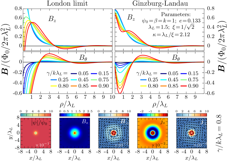
Figure 2: The upper row displays the longitudinal ($B_{z}$) and circular ($B_{\theta}$) components of the magnetic field of a single vortex, as functions of the radial distance $\rho$ from the vortex center, and for various values of the parity-odd coupling $\gamma$. The left and right panels show the magnetic field in the London limit and beyond the London approximation, respectively. The panels in the bottom row, result from the minimization of the Ginzburg-Landau free energy at the parity-breaking coupling $\gamma=0.8\gamma_{\star}$. They show the superconducting condensate $|\psi|$, the longitudinal and transverse components of the magnetic field, $B_{z}$ and ${\boldsymbol{B}}_{\perp}$, and currents , $j_{z}$ and ${\boldsymbol{j}}_{\perp}$, in the transverse plane of the vortex. In the case of a weak parity violation, $\gamma\ll\gamma_{\star}$, the longitudinal component of the magnetic field is similar to that of conventional Abrikosov vortices for which $B_{z}(\rho)$ is monotonic and exponentially localized around the vortex core at $\rho=0$. When the parity-breaking term becomes large, with $\gamma$ approaching the critical value $\gamma_{\star}$, the longitudinal component $B_{z}$ becomes a non-monotonic function as the distance $\rho$ from the vortex core increases.

Thus, the vortex field ${\boldsymbol{v}}$ completely determines, via its Fourier image ${\boldsymbol{v}}_{\boldsymbol{p}}$, the momentum-space representations of the current (13) and of the magnetic field (14). The corresponding real-space solutions are obtained by the Fourier transformation (12). Assuming the translation invariance along the $z$-axis, a set of $N$ vortices located at the positions $\tilde{\boldsymbol{x}}_{a}$, and characterized by the individual winding numbers $n_{a}$ (with $a=1,\cdots,N$), is described by the Fourier components

$${\boldsymbol{v}}_{\boldsymbol{p}}=2\pi\frac{\delta(p_{z}){\boldsymbol{\mathrm{e}}}_{z}}{\lambda_{L}^{2}}\sum_{a=1}^{N}n_{a}\text{e}^{-i{\boldsymbol{p}}\cdot\tilde{\boldsymbol{x}}_{a}}\,,$$ (15)

where the Dirac delta for the momentum $p_{z}$ specifies the translation invariance of the configuration.

III.2 Single vortex

The analysis becomes particularly simple for a single elementary vortex with a unit winding number ($n_{1}{=}1$) located at the origin ($\boldsymbol{x}_{1}=0$). The corresponding magnetic field reads as follows:

$${\boldsymbol{B}}_{\boldsymbol{p}}=\frac{2\pi\Phi_{0}\delta(p_{z})}{\lambda_{L}^{2}\Sigma}\left(\begin{array}[]{c}\phantom{-}i\Gamma(1-{\boldsymbol{p}}^{2})p_{y}\\ -i\Gamma(1-{\boldsymbol{p}}^{2})p_{x}\\ (1-2\Gamma^{2}){\boldsymbol{p}}^{2}+1\end{array}\right).$$ (16)

Next, we express the position, $\tilde{\boldsymbol{x}}=(\tilde{\rho}\cos\theta,\tilde{\rho}\sin\theta,\tilde{z})$, and momentum, ${\boldsymbol{p}}=(q\cos\vartheta,q\sin\vartheta,p_{z})$, in cylindrical coordinates. An integration over the angular degrees of freedom $\vartheta$ nullifies the radial part $B_{\rho}$ of the magnetic field and generates the Bessel functions of the first kind, $J_{0}$ and $J_{1}$. Hence, the nonzero components of the magnetic field can be expressed as one-dimensional integrals over the radial momentum $q$:

$$B_{\theta}\Big{(}\frac{\rho}{\lambda_{L}}\Big{)}\!=\!\frac{\Phi_{0}\Gamma}{2\pi\lambda_{L}^{2}}\int_{0}^{\infty}\!\frac{q^{2}(1-q^{2})dq}{(1+q^{2})^{2}-4\Gamma^{2}q^{2}}J_{1}\Big{(}\frac{q\rho}{\lambda_{L}}\Big{)}\,,$$

$$B_{z}\Big{(}\frac{\rho}{\lambda_{L}}\Big{)}\!\!=\!\frac{\Phi_{0}}{2\pi\lambda_{L}^{2}}\!\int_{0}^{\infty}\!\!\frac{q[(1-2\Gamma^{2})q^{2}+1]dq}{(1+q^{2})^{2}-4\Gamma^{2}q^{2}}J_{0}\Big{(}\frac{q\rho}{\lambda_{L}}\Big{)}.$$ (17)

Similarly, the nonzero components of the current are:

$$j_{\theta}\Big{(}\frac{\rho}{\lambda_{L}}\Big{)}\!=\!\frac{\Phi_{0}}{8\pi^{2}k\lambda_{L}^{3}}\int_{0}^{\infty}\!\frac{q^{2}(q^{2}+1-2\Gamma^{2})dq}{(1+q^{2})^{2}-4\Gamma^{2}q^{2}}J_{1}\Big{(}\frac{q\rho}{\lambda_{L}}\Big{)}\,,$$

$$j_{z}\Big{(}\frac{\rho}{\lambda_{L}}\Big{)}\!\!=\!\frac{-\Phi_{0}\Gamma}{8\pi^{2}k\lambda_{L}^{3}}\!\int_{0}^{\infty}\!\!\frac{q(1-q^{2})dq}{(1+q^{2})^{2}-4\Gamma^{2}q^{2}}J_{0}\Big{(}\frac{q\rho}{\lambda_{L}}\Big{)}.$$ (18)

Using the Hankel transform Piessens (2018), as demonstrated in detail in Appendix D, these integrals can be solved analytically in terms of the modified Bessel functions of the second kind $K_{\nu}$. Introducing the complex number $\eta=\Gamma-i\sqrt{1-\Gamma^{2}}$, the nonzero components of the magnetic field read

$$B_{\theta}\Big{(}\frac{\rho}{\lambda_{L}}\Big{)}\!=\!\frac{\Phi_{0}}{2\pi\lambda_{L}^{2}}\mathrm{Re}\left[i\eta^{2}K_{1}\left(\frac{i\eta\rho}{\lambda_{L}}\right)\right]\,,$$

$$B_{z}\Big{(}\frac{\rho}{\lambda_{L}}\Big{)}\!\!=\!\frac{-\Phi_{0}}{2\pi\lambda_{L}^{2}}\!\mathrm{Re}\left[\eta^{2}K_{0}\left(\frac{i\eta\rho}{\lambda_{L}}\right)\right]\,.$$ (19)

Similarly, the nonzero components of ${\boldsymbol{j}}$ are:

$$j_{\theta}\Big{(}\frac{\rho}{\lambda_{L}}\Big{)}\!=\!\frac{-\Phi_{0}}{8\pi^{2}k\lambda_{L}^{3}}\mathrm{Re}\left[i\eta K_{1}\left(\frac{i\eta\rho}{\lambda_{L}}\right)\right]\,,$$

$$j_{z}\Big{(}\frac{\rho}{\lambda_{L}}\Big{)}\!\!=\!\frac{\Phi_{0}}{8\pi^{2}k\lambda_{L}^{3}}\!\mathrm{Re}\left[\eta K_{0}\left(\frac{i\eta\rho}{\lambda_{L}}\right)\right]\,.$$ (20)

In the absence of parity breaking ($\Gamma=0$ and $\eta=-i$), the above integrals expectedly give the textbook expressions for the nonvanishing components of the magnetic field, $B_{z}(\rho/\lambda_{L})\!=\!\frac{\Phi_{0}}{2\pi\lambda_{L}^{2}}K_{0}(\rho/\lambda_{L})$, and of the superconducting current, $4\pi kj_{\theta}(\rho/\lambda_{L})\!=\!\frac{\Phi_{0}}{2\pi\lambda_{L}^{3}}K_{1}(\rho/\lambda_{L})$.

Figure 2 shows the magnetic field of a single vortex both in the London limit and for the full Ginzburg-Landau problem. First, although the solutions are expected to differ at the vortex core, the overall behavior remains qualitatively similar in both cases. Indeed, the London solutions are divergent at the vortex core, and thus they require a sharp cut-off at the coherence length $\xi$. Solutions beyond the London limit, on the other hand, are regular everywhere. The bottom row of Fig. 2 shows a typical vortex solution obtained numerically beyond the London limit. This is a close-up view of the vortex core structure, while the actual numerical domain is much larger in order to prevent any finite-size effect. While the density profile is similar to that of common vortices, the magnetic field shows a pretty unusual profile featuring a slight inversion, away from the center. For the current parameter set, where $\gamma=0.8\gamma_{\star}$, the amplitude of the reversed field compared to the maximal amplitude is rather small. Yet, as illustrated on the top-right panels of Fig. 2, the amplitude of inversion of the magnetic field, typically increases with the parity-breaking coupling $\gamma$. Thus when $\gamma$ is close to the critical coupling $\gamma_{\star}$, the magnitude of the responses and field inversions become more important.

When the parity-breaking coupling $\gamma$ is small compared to the upper bound $\gamma_{\star}$, the longitudinal component $B_{z}$ of the magnetic field is monotonic and exponentially localized, as for conventional vortices. The vortex configurations start to deviate from the conventional case when the parity breaking strengthens. Indeed, when $\gamma$ increases, the magnetic field $B_{z}$ does not vary monotonically any longer. As can be seen in the top-right panel of Fig. 2, it can be reversed, and even features several local minima as $\gamma$ approaches its critical value $\gamma_{\star}$. Note that, the complicated spatial structure and inversion of the magnetic field also comes with the inversion of the supercurrents. The distance from the vortex center $\rho\simeq 4\lambda_{L}$, where the longitudinal component of the magnetic field first vanishes, corresponds to the radius where the in-plane current $j_{\theta}$ reverses its sign. Similarly, the longitudinal current $j_{z}$ vanishes for the first time at the shorter distance to the vortex core, $\rho\simeq 2\lambda_{L}$, where the circular magnetic field cancels, $B_{\theta}=0$. These observations are consistent with the results from the perturbative regime, $\gamma\ll\gamma_{\star}$ Kashyap and Agterberg (2013). Interestingly, these specific radii are pretty much unaffected by the value of the parity-breaking coupling.

Note that the structure of the zeros of the modified Bessel functions with complex arguments shows that any non-zero value of the parity-breaking coupling $\gamma$ exhibits zeros at some distance away from the singularity. In practice, for small values of $\gamma$, the first zero is pushed very far from the vortex core, and the amplitude of the field inversion is vanishingly small. Hence while the field inversion formally occurs at all finite $\gamma$, it becomes noticeable when $\gamma$ is not too small. The structure of magnetic field inversion as a function of $\gamma$ qualitatively resembles the alternating attractive/positive regions displayed in the right panel of Fig. 3.

IV Vortex interactions

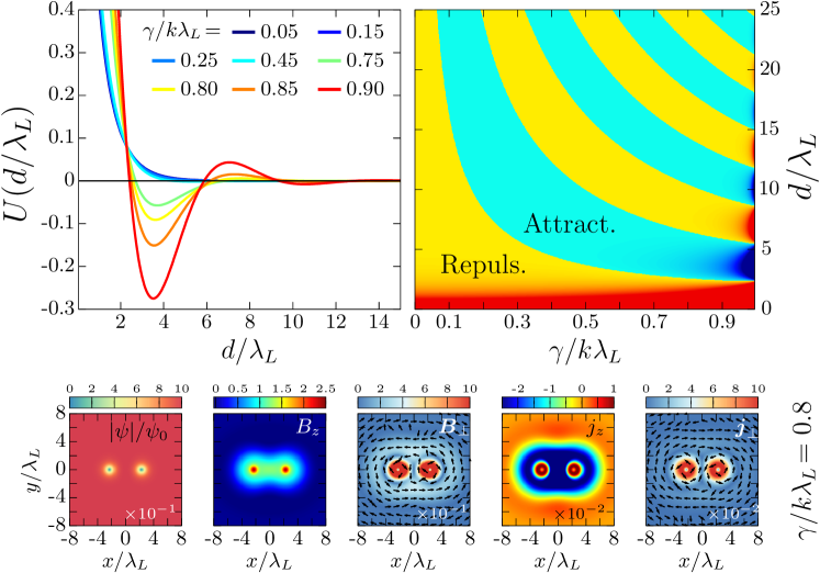
Figure 3: The top-left panel shows the function $U(d/\lambda_{L})$ that controls the intervortex interactions, as a function of the distance $d$ between the vortices, for various values of the parity-odd coupling $\gamma$. The top-right panel displays a phase diagram showing the attractive (blue) and repulsive (yellow) regions depending on the parity breaking coupling $\gamma$ and the intervortex distance $d$. The panels in the top row corresponds to the London limit. The panels on the bottom row, obtained within the Ginzburg-Landau calculation, show various physical quantities in the transverse plane of a vortex bound state, for the parity-breaking coupling $\gamma=0.8\gamma_{\star}$ (the other parameters are the same as in Fig. 2). This vortex pair, obtained after convergence of minimization of the Ginzburg-Landau free energy, demonstrates that the property of the non-monotonic interactions can survive beyond the London limit. The London limit estimates the intervortex separation $d_{LL}=3.6\lambda_{L}$, while the Ginzburg-Landau calculation finds $d_{GL}=4.6\lambda_{L}$. Despite the fact that the GL simulation is far from the London limit (here $\kappa=2.12$), both values are in qualitative agreement.

The possibility of having an inversion of the magnetic field suggests that the interaction between two vortices might be much more involved than the pure repulsion that occurs in conventional type-2 superconductors. Indeed, since the conventional long-range intervortex repulsion is due to the magnetic field, it is quite likely that the interaction here might be not only quantitatively, but also qualitatively altered. To investigate these, we consider the London limit free energy $F$ written in the previously used dimensionless coordinates. Using Eq. (12) to express the quantities ${\boldsymbol{j}}$ and ${\boldsymbol{B}}$ in terms of their Fourier components, we find the expression of the free energy in the momentum space:

$$F=\frac{\lambda_{L}^{3}}{8\pi}\int\frac{d^{3}{\boldsymbol{p}}}{(2\pi)^{3}}\Big{\{} {\boldsymbol{B}}_{\boldsymbol{p}}\cdot{\boldsymbol{B}}_{-{\boldsymbol{p}}}+(4\pi k\lambda_{L}{\boldsymbol{j}}_{\boldsymbol{p}})\cdot(4\pi k\lambda_{L}{\boldsymbol{j}}_{-{\boldsymbol{p}}})$$

$$+2\Gamma(4\pi k\lambda_{L}{\boldsymbol{j}}_{\boldsymbol{p}})\cdot{\boldsymbol{B}}_{-{\boldsymbol{p}}}\Big{\}}\,.$$ (21)

Replacing the Fourier components of the magnetic field ${\boldsymbol{B}}_{\boldsymbol{p}}$ and of the current ${\boldsymbol{j}}_{\boldsymbol{p}}$ with the corresponding expressions in terms of the vortex field ${\boldsymbol{v}}_{\boldsymbol{p}}$, Eqs. (13) and (14), respectively, yields the free energy:

$$\leavevmode\nobreak\ \leavevmode\nobreak\ \leavevmode\nobreak\ \leavevmode\nobreak\ F=\frac{\lambda_{L}^{3}}{8\pi}\int\frac{d^{3}{\boldsymbol{p}}}{(2\pi)^{3}}\,{\boldsymbol{v}}_{\boldsymbol{p}}^{m}G^{mn}{\boldsymbol{v}}_{-{\boldsymbol{p}}}^{n}$$ (22)

$$\text{where}\leavevmode\nobreak\ G^{mn}=\Upsilon^{lm}_{\boldsymbol{p}}\Upsilon^{ln}_{-{\boldsymbol{p}}}+\Lambda^{lm}_{\boldsymbol{p}}\Lambda^{ln}_{-{\boldsymbol{p}}}+2\Gamma\Lambda^{lm}_{\boldsymbol{p}}\Upsilon^{ln}_{-{\boldsymbol{p}}}\,.$$

The interaction matrix $G$ has a rather involved structure. Yet, given that only the axial Fourier components of the vortex field (15) are nonzero, only the component $G^{zz}$ will contribute to the energy. Up to terms that are proportional to $p_{z}$, and thus will be suppressed by the Dirac delta $\delta(p_{z})$, $G^{zz}$ takes the simple form

$$G^{zz}=\frac{(1-\Gamma^{2})(1+{\boldsymbol{p}}^{2})}{\Sigma}\leavevmode\nobreak\ +\leavevmode\nobreak\ (\text{terms}\propto p_{z})\,.$$ (23)

Finally, using the vortex field ansatz (15), together with the expressions (22) and (23) determines the free energy associated with a set of translationally invariant vortices

$$F=\frac{\Phi_{0}^{2}(1{-}\Gamma^{2})}{8\pi\lambda_{L}}\sum_{a,b=1}^{N}n_{a}n_{b}\!\int\!\frac{d^{2}{\boldsymbol{p}}}{2\pi}\frac{1+{\boldsymbol{p}}^{2}}{\Sigma({\boldsymbol{p}}^{2})}\text{e}^{i{\boldsymbol{p}}\cdot(\tilde{\boldsymbol{x}}_{a}-\tilde{\boldsymbol{x}}_{b})}.$$ (24)

The two dimensional integration in (24) can further be simplified and finally, the free energy reads as:

$$F=\frac{\Phi_{0}^{2}(1-\Gamma^{2})}{8\pi\lambda_{L}} \sum_{a,b=1}^{N}n_{a}n_{b}U\left(\frac{|x_{a}-x_{b}|}{\lambda_{L}}\right)$$ (25)

$$\text{where}\leavevmode\nobreak\ \leavevmode\nobreak\ U(x) =\int_{0}^{\infty}\!\frac{q(1+q^{2})\,dq}{(1+q^{2})^{2}-4\Gamma^{2}q^{2}}\,J_{0}(qx)$$

$$=\mathrm{Re}\left[\frac{i\eta}{\sqrt{1-\Gamma^{2}}}K_{0}\left(i\eta x\right)\right]\,.$$ (26)

Hence the free energy of a set of vortices reads as:

$$F=F_{0}+\frac{\Phi_{0}^{2}(1-\Gamma^{2})}{4\pi\lambda_{L}}\sum_{a,b>a}^{N}n_{a}n_{b}U\left(\frac{|x_{a}-x_{b}|}{\lambda_{L}}\right)\,,$$ (27)

where the term $F_{0}=\frac{\Phi_{0}^{2}(1-\Gamma^{2})}{8\pi\lambda_{L}}\sum_{a}n_{a}^{2}U(\xi)$ accounts for the self-energy of individual vortices. Since $U(x)$ diverges at small separations $x$, the self-energy has to be regularized at the coherence length $\xi\ll\lambda_{L}$, which determines the size of the vortex core. The interaction energy of the vortices separated by a distance $d$ is thus determined by the function $U(d/\lambda_{L})$. In the absence of parity breaking ($\Gamma=0$ and $\eta=-i$), Eq. (27) leads again to the textbook expression for the interaction energy $V_{\mathrm{int}}(d/\lambda_{L})=\Phi_{0}^{2}K_{0}(d/\lambda_{L})/4\pi\lambda_{L}$.

Figure 3 displays the function $U(d/\lambda_{L})$, which controls the interacting potential between vortices, calculated in the London limit. For vanishing $\gamma$, the interaction is purely repulsive, and it is altered by a nonzero coupling. As shown in the left panel, when increasing $\gamma/k\lambda_{L}$ the interaction can become non-monotonic with a minimum at a finite distance of about $4\lambda_{L}$. Upon further increase of the coupling $\gamma$ toward the critical coupling $\gamma_{\star}$, the interacting potential can even develop several local minima. The phase diagram on the right panel of Fig. 3 shows the different attractive and repulsive regions as functions of $\gamma$ and of the vortex separation.

The fact that the interaction energy features a minimum at a finite distance implies that a pair of vortices tends to form a bound state. As can be seen in the bottom row of Fig. 3, the tendency of vortices to form bound-states persists beyond the London approximation. This configuration is obtained numerically by minimizing the Ginzburg-Landau free energy (1). Notice that these bottom panels show a close-up view of the vortex pair, while the actual numerical domain is much larger . The formation of a vortex bound state can heuristically be understood as a compromise between the axial magnetic repulsion of $B_{z}$ which competes with in-plane attraction mediated by $B_{\perp}$. The bound-state formation can alternatively be understood to originate from the competition between the in-plane and axial contributions of the currents. First of all, the in-plane screening currents mediate, as usual, repulsion between vortices. The interaction between the axial components of the currents, on the other hand, mediates an attraction, just like the force between parallel wires carrying co-directed electric currents.

The non-monotonic behavior of the magnetic field and currents thus leads to non-monotonic intervortex interactions, and therefore allows for bound-states of vortices or clusters to form. Such a situation is known to exist in multicomponent superconductors due to the competition between various length scales (see e.g. Babaev and Speight (2005); Babaev et al. (2012); Carlström et al. (2011); Babaev et al. (2017); Silaev et al. (2018) as well as Haber and Schmitt (2017, 2018) for superconducting/superfluid systems). In an applied external field, the existence of non-monotonic interactions allows for a macroscopic phase separation into domains of vortex clusters and vortex-less Meissner domains. The situation here contrasts with the multicomponent case, as it occurs only due to the existence of Lifshitz invariants. In two-dimensional systems of interacting particles, multi-scale potentials and non-monotonic interactions are known to be responsible for the formation of rich hierarchical structures. These structures include clusters of clusters, concentric rings, clusters inside a ring, or stripes Olson Reichhardt et al. (2010); Varney et al. (2013). It can thus be expected that very rich structures would appear in noncentrosymmetric superconductors as well. However, a verification of this conjecture is beyond the scope of the current work, as it deserves a separate detailed investigation.

As shown in Fig. 3, the interaction energy $V_{v/v}(x)\propto U(x)$ between two vortices with unit winding $n_{1}=n_{2}=1$ can thus lead to the formation of a vortex bound state. A very interesting property is that it also opens the possibility of vortex/anti-vortex bound-states. Indeed, according to Eq. (27) the interaction of a vortex $n_{1}=1$ and an anti-vortex $n_{2}=-1$ corresponds to a reversal of the interacting potential: $V_{v/av}(x)\propto-U(x)$. Thus from Fig. 3 it is clear that if a vortex/anti-vortex pair is small enough, it will collapse to zero and thus lead to the vortex/anti-vortex annihilation. Now, considering for example the curve $\gamma/k\lambda_{L}=0.9$ in Fig. 3, if the size of the vortex/anti-vortex pair is larger than $4\lambda_{L}$, there exists an energy barrier that prevents the pair from further collapse. Hence the vortex/anti-vortex pair should relax to a local minimum of the interaction energy. The resulting vortex/anti-vortex bound state has thus a size of approximately $7\lambda_{L}$. Note that the above analysis demonstrates that vortex/anti-vortex bound-states do exist as meta-stable states in the London limit. It is quite likely that these results are still qualitatively valid beyond the London approximation at least for strong type-2 superconductors. The possibility to realize vortex/anti-vortex pairs for weakly type-2 superconductors requires careful analysis and is beyond the scope of the current work.

V Conclusions

In this paper we have demonstrated that the vortices in noncentrosymmetric cubic superconductors feature unusual properties induced by the possible reversal of the magnetic field around them. Indeed, the longitudinal (i.e., parallel to the vortex line) component of the magnetic field changes sign at a certain distance away from the vortex core. Contrary to the vortices in a conventional superconductor, the magnetic-field reversal in the parity-broken superconductor leads to non-monotonic intervortex forces which can act both attractively and repulsively depending on the distance separating individual vortices.

These properties have been demonstrated analytically within the London limit. Our numerical analysis of the nonlinear Ginzburg-Landau theory proves that the magnetic-field reversal and the non-monotonic intervortex forces survive beyond the London approximation in noncentrosymmetric superconductors.

Due to the nonmonotonic intervortex interactions, the vortices in the parity-breaking superconductors may form unusual states of vortex matter, such as bound states and clusters of vortices. The structure of the interaction potential strongly suggests that very rich vortex matter structures can emerge. For example, hierarchically structured quasi-regular vortex clusters, stripes and more, are typical features of the interacting multi-scale and non-monotonic interaction potentials Olson Reichhardt et al. (2010); Varney et al. (2013). Moreover, given the possibility to form vortex/anti-vortex bound states, we can anticipate important consequences for the statistical properties and phase transitions in such models.

Note added: In the process of completion of this work, we were informed about an independent work by Samoilenka and Babaev Samoilenka and Babaev (2020) showing similar results about vortices and their interactions. The submission of this work was coordinated with that of Samoilenka and Babaev (2020).

Appendix A Positive definiteness of the energy

The free energy (1) should be bounded from below in order to be able to describe the ground state of the NCS superconductor. To demonstrate the boundedness, we use the relations

$${\boldsymbol{j}} =2e|\psi|^{2}\left({\boldsymbol{\nabla}}\varphi-e{\boldsymbol{A}}\right),$$ (A1a)

$$|{\boldsymbol{D}}\psi|^{2} =\left({\boldsymbol{\nabla}}|\psi|\right)^{2}+|\psi|^{2}\left({\boldsymbol{\nabla}}\varphi-e{\boldsymbol{A}}\right)^{2}\,$$ (A1b)

$$=\left({\boldsymbol{\nabla}}|\psi|\right)^{2}+\frac{|{\boldsymbol{j}}|^{2}}{4e^{2}|\psi|^{2}}\,,$$ (A1c)

to rewrite the energy density in the following form:

$$\mathcal{F} =\frac{{\boldsymbol{B}}^{2}}{8\pi}+k\left({\boldsymbol{\nabla}}|\psi|\right)^{2}+\frac{k|{\boldsymbol{j}}|^{2}}{4e^{2}|\psi|^{2}}+\gamma{\boldsymbol{j}}\cdot{\boldsymbol{B}}+V[\psi]$$ (A2a)

$$=\frac{1}{8\pi}\left[{\boldsymbol{B}}^{2}+8\pi\gamma{\boldsymbol{j}}\cdot{\boldsymbol{B}}\right]+\frac{k|{\boldsymbol{j}}|^{2}}{4e^{2}|\psi|^{2}}$$

$$\leavevmode\nobreak\ \leavevmode\nobreak\ \leavevmode\nobreak\ \leavevmode\nobreak\ \leavevmode\nobreak\ \leavevmode\nobreak\ +k\left({\boldsymbol{\nabla}}|\psi|\right)^{2}+\frac{\beta}{2}(|\psi|^{2}-\psi_{0}^{2})^{2}$$ (A2b)

$$=\frac{1}{8\pi}\big{|}{\boldsymbol{B}}+4\pi\gamma{\boldsymbol{j}}\big{|}^{2}+\Big{(}\frac{k}{4e^{2}|\psi|^{2}}-2\pi\gamma^{2}\Big{)}|{\boldsymbol{j}}|^{2}$$

$$\leavevmode\nobreak\ \leavevmode\nobreak\ \leavevmode\nobreak\ \leavevmode\nobreak\ \leavevmode\nobreak\ \leavevmode\nobreak\ +k\left({\boldsymbol{\nabla}}|\psi|\right)^{2}+\frac{\beta}{2}(|\psi|^{2}-\psi_{0}^{2})^{2}\,.$$ (A2c)

Leaving aside all terms with the perfect squares in Eq. (A2c), we find that the only criterion for the free energy to be bounded from below is to require the prefactor in front of the $|{\boldsymbol{j}}|^{2}$ term to be positive. We arrive at the following condition of the stability of the system (1):

$$\gamma^{2}<\frac{k}{8\pi e^{2}|\psi|^{2}}\,.$$ (A3)

In the ground state with $|\psi|=\psi_{0}$, the stability condition (A3) reduces to the simple inequality:

$$\gamma<\gamma_{\star}=k\lambda_{L}\,.$$ (A4)

where $\lambda_{L}$ is the London penetration depth (4).

In the London limit, the superconducting density $|\psi|^{2}$ is a fixed constant quantity regardless of the external conditions. Therefore, the Ginzburg-Landau theory for the NCS superconductor in the London limit is always bounded from below provided the Lifshitz–invariant coupling $\gamma$ satisfies Eq. (A4).

Positive definiteness beyond the London limit

The issue of positive definiteness is less obvious beyond the London limit. Indeed, let us first assume that the values of the parameters $(e,k,\gamma)$ are chosen in such a way that the formal criterium (A3) is satisfied. If we neglect the fluctuations of the condensate $\psi$ (this requirement is always satisfied in the London regime) then we indeed find that the ground state resides in a locally stable regime so that all terms in the free energy (A2c) are positively defined. However, the density $|\psi|$ is, in principle, allowed to take any value, and large enough fluctuations of $|\psi|$ might trigger an instability. A possible signature of the instability can indeed be spotted in the property that a variation of the absolute value of the condensate about the ground state, $|\psi|=\psi_{0}+\delta|\psi|$, gives a negative contribution to the free energy, $\delta F=-k\delta|\psi|/(2e^{2}\psi_{0}^{3})$, in the linear order, provided all other parameters are fixed.

To illustrate a possible mechanism of the development of the instability inside the noncentrosymmetric superconductor, let us consider a large enough local region characterized by a uniform, coordinate-independent condensate $\psi$. For this configuration, the third (gradient) term in the free-energy density (A2c) is identically zero. Gradually increasing the value of the condensate beyond the ground state value $\psi_{0}$, we increase the fourth (potential) term in Eq. (A2c), which make this change energetically unfavorable. On the other hand, as the condensate crosses the threshold of applicability of Eq. (A3), then the second term in the free energy (A2c) becomes negatively defined, and the development of the current ${{\boldsymbol{j}}}$ leads to the unbounded decrease of this term. The rise in the current ${\boldsymbol{j}}$ will, in turn, affect the first (magnetic) term, which may be compensated by a rearranging of the magnetic field ${\boldsymbol{B}}$ with the local environment in such a way that the combination ${\boldsymbol{B}}+4\pi\gamma{\boldsymbol{j}}$ keeps a small value in the discussed region.

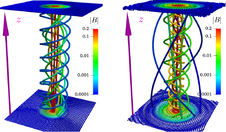
Figure 4: Helical structure of the magnetic field streamlines around vortices in noncentrosymmetric superconductors. The magnetic field is displayed on the two planes normal with respect to the vortex line. The colors encode the amplitude $|B|$, while the arrows demonstrate the orientation of the field. The tubes represent streamlines of the magnetic field between both planes. The left panel shows the helical structure of the streamlines for a moderate value of the parity-breaking coupling, $\gamma/k\lambda=0.2$. The streamlines here feature all the same chirality. The right panel corresponds to rather important parity-breaking coupling $\gamma/k\lambda=0.8$, for which the longitudinal component of the magnetic field is inverted at some distance from the core. The chirality of the streamline depends on whether the longitudinal component of the magnetic field is inverted.

Notice that the presence of isolated vortices makes the system stable as in a vortex core the condensate vanishes, $\psi\to 0$, and the second, potentially unbounded term in (A2c) becomes positively defined. In our numerical simulations, we were also spotting certain unstable patterns especially in the regimes when the Lifshitz-invariant coupling $\gamma$ was chosen to close to the critical value $\gamma_{\star}$ in the ground state (A4). For example, a system of randomly placed multiple elementary vortices relaxes their free energy via mutual attraction and the formation of a common bound state. Since the vortex bound state hosts a stronger circular electric current, it becomes possible to overcome the stability by ‘compressing’ the vortex cluster, and then destabilizing the whole system.

We conclude that the processes that permit fluctuations of the condensate $|\psi|$ towards the large values (as compared to the ground-state value $\psi_{0}$) could activate the destabilization of the whole model. Theoretically, the unboundedness of the free energy from below may appear to be an unwanted feature of the model. However, one should always keep in mind that the Ginzburg-Landau functional is a leading part of the gradient expansion of an effective model, and there always exist higher power gradients that will play a stabilizing role preventing the unboundedness from actually being realized in a physically relevant model.

Appendix B Vortex helicity

As emphasized in the main body of the paper, the magnetic field of vortex states in cubic noncentrosymmetric superconductors features a helicoidal structure around the core. This is illustrated in Fig. 4, which displays a typical magnetic field structure around vortex cores. The magnetic field there is determined within the London approximation (III.2). Each helical tube represents a streamline of the magnetic field which is tangent to the magnetic field in every point. Fig. 4 clearly shows that every streamline forms an helix along the axis $z$. Each helix has a period that depends on the distance from the helix to the center of the vortex. The latter property indicates that, contrary to the magnetic field itself, the streamlines of the magnetic field are not invariant for the translations along the $z$ axis.

Fig. 4 shows two qualitatively different situation of moderate (left panel) and important (right panel) parity-breaking coupling $\gamma$. For moderate parity-breaking coupling, the magnetic field streamlines have a helical structure with a pitch that varies with the distance from the vortex core. Note that all streamlines have the same chirality, which is specified by the sign of the parity-breaking coupling $\gamma$. On the other hand, as discussed in the main body of the paper, vortices feature inversion of the magnetic field ${\boldsymbol{B}}$ for important parity-breaking coupling $\gamma$. As a result, the chirality of the streamline depends on whether the longitudinal component of the magnetic field is inverted. More details about the helical structure of the magnetic field can be seen from animations in the supplemental material Sup .

Appendix C Description of the supplementary animations (see ancillary files)

There are three animations that illustrate the results of presented in the manuscript. The magnetic field forms helical patterns around a straight static vortex, in a noncentrosymmetric superconductor. For important values of the parity-breaking coupling $\gamma$, the magnetic field ${\boldsymbol{B}}$ can further show inversion patterns around the vortex. That is, as the distance from the vortex core increases, the longitudinal component of the magnetic field may change it sign.

The supplementary animations display the following: On the two static planes, normal with respect to the vortex line, the colors encode the amplitude of the magnetic field B, while the arrows demonstrate the orientation of the field. The tubes represent streamlines of the magnetic magnetic field between both planes.

• movie-1.avi and movie-2.avi: Helical structure of the magnetic field streamlines around vortices in noncentrosymmetric superconductors. The fisrt movie (movie-1.avi) shows the helical structure of the streamlines for moderate value of the parity-breaking coupling $\gamma/k\lambda=0.2$. The streamlines here feature all the same chirality. The second animation (movie-2.avi) corresponds to rather important parity-breaking coupling $\gamma/k\lambda=0.8$, for which the longitudinal component of the magnetic field is inverted at some distance from the core. The chirality of the streamline depends on whether the longitudinal component of the magnetic field is inverted. That is depending on the chirality, some of the streamlines propagate forward (along positive $z$-direction), while other propagate backward (along negative $z$- direction).

• movie-3.avi: Magnetic streamlines, emphasizing forward propagating lines (solid tubes), in the case of field inversion due to important parity-breaking coupling $\gamma/k\lambda=0.8$. The transparent tubes propagate backward (along the negative $z$-direction).

• movie-4.avi: Magnetic streamlines, emphasizing backward propagating lines (solid tubes), in the case of field inversion due to important parity-breaking coupling $\gamma/k\lambda=0.8$. The transparent tubes propagate forward (along the positive $z$-direction).

Appendix D Calculation of the integrals

The intervortex interaction (26), the components of the magnetic field (III.2), and the components of the current (III.2) are expressed in terms of integrals of the generic form

$$G_{\nu}(x)\!=\!\int_{0}^{\infty}\!\frac{P(q)}{(1+q^{2})^{2}-4\Gamma^{2}q^{2}}q^{\nu+1}J_{\nu}(qx)dq\,,$$ (D5)

where $\nu=0,1$. Introducing the complex number $\eta=\Gamma-i\sqrt{1-\Gamma^{2}}$, the quotient of the polynomials $P(q)$ and $(1+q^{2})^{2}-4\Gamma^{2}q^{2}$ can be written as

$$\frac{P(q)}{(1+q^{2})^{2}-4\Gamma^{2}q^{2}}=\frac{C}{q^{2}-\eta^{2}}+\frac{C^{*}}{q^{2}-\eta^{*2}}\,,$$ (D6)

where ^∗ stands for the complex conjugation (since $q$ is real). The coefficient $C$ is the solution of the equation

$$P(q)=C(q^{2}-\eta^{*2})+C^{*}(q^{2}-\eta^{2})\,.$$ (D7)

The integral (D5) becomes as follows:

$$G_{\nu}(x) =2\int_{0}^{\infty}\!\mathrm{Re}\left[\frac{C}{q^{2}-\eta^{2}}\right]q^{\nu+1}J_{\nu}(qx)dq$$

$$=2\mathrm{Re}\left[C\int_{0}^{\infty}\!\frac{q^{\nu}}{q^{2}-\eta^{2}}J_{\nu}(qx)qdq\right]\,.$$ (D8)

The integral in (D) has a form of an Hankel transform Piessens (2018) which is an integral transformation whose kernel is a Bessel function. In short, the $\nu$-th Hankel transform $F_{\nu}$ of a given function $f(q)$ with $q>0$ is defined as

$$F_{\nu}(x):=\int_{0}^{\infty}f(q)J_{\nu}(qx)qdq\,.$$ (D9)

The inverse of the Hankel transform is also a Hankel transform. The functions

$$f(q)=\frac{q^{\nu}}{q^{2}+a^{2}}\leavevmode\nobreak\ \leavevmode\nobreak\ \leavevmode\nobreak\ \longleftrightarrow\leavevmode\nobreak\ \leavevmode\nobreak\ \leavevmode\nobreak\ F_{\nu}(x)=a^{\nu}K_{\nu}(ax)\,,$$ (D10)

are related to each other via the Hankel transformation (D9). Identifying $a=i\eta$, the integral in (D) thus read as

$$\int_{0}^{\infty}\!\frac{q^{\nu}}{q^{2}-\eta^{2}}J_{\nu}(qx)qdq=(i\eta)^{\nu}K_{\nu}(i\eta x)\,.$$ (D11)

This is a well-defined expression since the constant $\eta$ is a complex number and the integral does not cross any pole. As a result, the integral (D5) reads as follows:

$$G_{\nu}(x)=2\mathrm{Re}\left[C(i\eta)^{\nu}K_{\nu}(i\eta x)\right]\,.$$ (D12)

This generic relation determines both ${\boldsymbol{j}}$, the magnetic field ${\boldsymbol{B}}$ and the interaction $U(x)$. Notice that the modified Bessel function of the second kind in Eq. (D12) can be related to the Hankel function of first kind using the relation

$$K_{\nu}(z)=\frac{i}{2}\text{e}^{i\nu\pi/2}H_{\nu}^{(1)}(iz)\,,\leavevmode\nobreak\ \leavevmode\nobreak\ \text{if}\leavevmode\nobreak\ -\pi<\mathrm{arg}\,z\leq\pi/2\,.$$ (D13)

In our case, $z=i\eta x$ and therefore $\mathrm{arg}\,z\in[0,\pi/2]$. Below we calculate the potential $U(x)$ as an example.

Example: calculation of the interaction

The interaction $U(x)$, defined in the main body in equation (25), reads as

$$U(x) =\int_{0}^{\infty}\!\frac{P(q)}{(1+q^{2})^{2}-4\Gamma^{2}q^{2}}\,J_{0}(qx)qdq$$

$$\text{where}\leavevmode\nobreak\ \leavevmode\nobreak\ P(q) =1+q^{2}.$$ (D14)

Solving (D6) for the given polynomial $P(q)$, gives the coefficient $C=i\eta/(2\sqrt{1-\Gamma^{2}})$. The solution (D12) for this particular problem is thus

$$U(x)=\mathrm{Re}\left[\frac{i\eta}{\sqrt{1-\Gamma^{2}}}K_{0}\left(i\eta x\right)\right]\,.$$ (D15)

In the absence of parity-breaking $\Gamma=0$, $\eta=-i$. This provides the textbook expression for the interaction of vortices in the London limit: $U(x)=K_{0}(x)$. Similar calculations determine the solutions (III.2) and (III.2) for the components of ${\boldsymbol{B}}$ and ${\boldsymbol{j}}$.