Quantitative lower bounds to
the Euclidean and the Gaussian
Cheeger constants

Abstract.

We provide a quantitative lower bound to the Cheeger constant of a set $\Omega$ in both the Euclidean and the Gaussian settings in terms of suitable asymmetry indexes. We provide examples which show that these quantitative estimates are sharp.

This is a pre-print of an article published in Ann. Fenn. Math.. The final authenticated version is available online at: https://doi.org/10.5186/aasfm.2021.4666

1. Introduction

In the past years inequalities of geometric-functional type have been widely studied in the literature, a — far from complete — list is [21, 24, 26, 28] (isoperimetric inequalities), [19, 44] (anisotropic Wulff inequalities), [1, 2, 16] (Gaussian inequalities), [23, 30, 32] (Riesz inequalities), [13, 14, 15, 27, 45] (Sobolev inequalities), [6, 22, 29] (Faber–Krahn inequalities, see also [5] for an account on other quantitative spectral inequalities).

In this paper we are interested in providing quantitative estimates on the Cheeger constant both in the Euclidean and in the Gaussian setting. Given any open set $\Omega$, of finite, resp. Euclidean or Gaussian, measure, the constant is defined as, resp.,

$$h(\Omega):=\inf\left\{\,\frac{P(E)}{|E|}\,\right\},\qquad h_{\gamma}(\Omega):=\inf\left\{\,\frac{P_{\gamma}(E)}{\gamma(E)}\right\},$$ (1.1)

where the infima are taken among subsets $E\subset\Omega$ of positive, resp. Euclidean or Gaussian, measure. In (1.1), we denote by $P(\cdot)$ and $P_{\gamma}(\cdot)$, resp., the distributional Euclidean and Gaussian perimeter, while by $|\cdot|$ and $\gamma(\cdot)$, resp., the standard Lebesgue and Gaussian measure.

Sets attaining the above infima are known to exist and are called Cheeger sets, see for instance [38, 46] for the Euclidean case, and [11] for the Gaussian case (more general settings have been explored, see for instance [7, 43, 48]). The task of computing the constant and determining the shape of Cheeger sets is usually referred to as the Cheeger problem. The constant first appeared in [12] in a Riemannian setting as a mean to bound from below the first Dirichlet eigenvalue of the Laplace–Beltrami operator. Through the coarea formula it can be proven that the Euclidean constant $h(\Omega)$ provides a lower bound to the first Dirichlet eigenvalue of the Laplace operator, and analogously the Gaussian constant $h_{\gamma}(\Omega)$ to the first Dirichlet eigenvalue of the Ornstein–Uhlenbeck operator (i.e., $-\Delta(\cdot)+\langle x,\nabla(\cdot)\rangle$).

Since then, the Euclidean problem has been widely studied and it has appeared in many different contexts, such as capillarity problems [31, 41], spectral properties of the $p$-Laplacian [35], and landslide modeling [33] to name a few. The interested reader is referred to the surveys [38, 46] and the references therein. The Gaussian counterpart was studied in relation to the prescribed mean curvature problem [11] and to image processing [10].

It is of interest to provide estimates on the constants as there are no available formulas to directly compute them, but for very few classes of sets $\Omega$ limited to the Euclidean $2$-dimensional setting, see [36, 39, 40, 42, 49]. In higher dimensions, some very special cases are treated in [3, 8, 17, 37]. To give an upper bound to $h(\Omega)$ (resp., $h_{\gamma}(\Omega)$) it is enough to compute the ratio $P(E)/|E|$ (resp., $P_{\gamma}(E)/\gamma(E)$) for any competitor $E$, while establishing lower bounds exploits the relevant isoperimetric inequalities. Indeed, first, rough estimates on the constants are provided by

$$h(\Omega)\geq h(B_{\Omega}),\qquad h_{\gamma}(\Omega)\geq h_{\gamma}(H_{\Omega}),$$ (1.2)

where by $B_{\Omega}$ we denote the ball centered at the origin s.t. $|\Omega|=|B_{\Omega}|$, and by $H_{\Omega}$ any halfspace s.t. $\gamma(\Omega)=\gamma(H_{\Omega})$.

The isoperimetric inequalities have been proven in quantitative forms by establishing bounds through asymmetry indexes measuring the distance (in some suitable sense) of $\Omega$ from the isoperimetric set with the same measure. Then, it is natural to wonder if any improvement to (1.2) can be attained by exploiting these stronger inequalities and get lower bounds of the form

$$\frac{h(\Omega)-h(B_{\Omega})}{h(B_{\Omega})}\geq c(n)\iota(\Omega)$$ (1.3)

in the Euclidean case, and

$$h_{\gamma}(\Omega)-h_{\gamma}(H_{\Omega})\geq c(\gamma(\Omega))\iota_{\gamma}(\Omega)$$ (1.4)

in the Gaussian case, where $\iota(\Omega)$ and $\iota_{\gamma}(\Omega)$ are some suitable asymmetry indexes. These inequalities give an improved lower bound on the Cheeger constant for sets that are near the corresponding isoperimetric set.

We remark that there are two main differences in the Euclidean  (1.3) and the Gaussian (1.4) inequalities that we expect to prove. First, in the Euclidean case, the quantitative estimate is renormalized, while in the Gaussian it is not. This is so because the respective quantitative isoperimetric estimates are renormalized in the former setting and not in the latter. Second, the constant $c$ in the Euclidean case depends only on the dimension $n$, while in the Gaussian only on the measure of $\Omega$. Again, this is a known feature of the quantitative isoperimetric inequalities in the two different settings.

A first result in this direction has been proven in the Euclidean case in [29] with $\iota(\Omega)=\alpha^{3}(\Omega)$, where $\alpha$ is known as the Fraenkel asymmetry index. This was later refined in [20], with the exponent $2$ in place of $3$, i.e., $\iota(\Omega)=\alpha^{2}(\Omega)$, and this exponent is known to be sharp, i.e., no such inequality can hold with a smaller power of $\alpha$. Our first main result, Theorem 2.1, states that in the Euclidean case a stronger quantitative inequality holds, where the index is given by the Riesz asymmetry index. To the best of our knowledge, there are no previous results in the Gaussian case. In Theorem 3.1 we prove a sharp quantitative inequality of type (1.4) in terms of the Gaussian Fraenkel asymmetry. Then we consider a different index in terms of the barycenter, which was introduced in [1, 18], and prove a sharp quantitative inequality in terms of this in Theorem 3.2. Rather surprisingly the optimal dependence on the asymmetry in Theorem 3.2 is different than in the quantitative Gaussian isoperimetric inequality of [1] and it has a logarithmic dependence on the barycenter index as in [18].

The paper is organized into two independent sections. In Section 2 we study the Euclidean case (1.3) and in Section 3 the Gaussian one (1.4). Each section is self-contained and begins with relevant definitions, related isoperimetric inequalities and statements of the results. The proof of the theorems follows. Finally, each section is complemented with an example that shows that the quantitative inequalities are sharp.

2. Estimates in the Euclidean setting

In the Euclidean setting there are three quantitative isoperimetric inequalities available, in terms of the following three indexes:

$$\alpha(\Omega) :=\min_{y\in{\mathbb{R}}^{n}}\left\{\,\frac{|\Omega\Delta(B_{\Omega}+y)|}{|\Omega|}\,\right\},$$ (2.1)

$$\zeta(\Omega) :=\frac{1}{P(B_{\Omega})}\left(\int_{B_{\Omega}}\frac{\textrm{d}x}{|x|}-\max_{y\in{\mathbb{R}}^{n}}\int_{\Omega}\frac{\textrm{d}x}{|x-y|}\right)$$ (2.2)

$$\beta(\Omega) :=\min_{y\in{\mathbb{R}}^{n}}\left\{\,\left(\frac{1}{2P(B_{\Omega})}\int_{{\partial}^{*}\Omega}|\nu_{\Omega}(x)-\nu_{B_{\Omega}+y}(\pi_{y,\Omega}(x))|^{2}\,\textrm{d}\mathcal{H}^{n-1}(x)\right)^{\frac{1}{2}}\,\right\},$$ (2.3)

where $\pi_{y,\Omega}(x)$ is the projection of ${\mathbb{R}}^{n}\setminus\{y\}$ on the boundary of $B_{\Omega}+y$, i.e.,

$$\pi_{y,\Omega}(x):=y+r\frac{x-y}{|x-y|}\,, \forall x\neq y,$$

being $r$ the radius of $B_{\Omega}$. Indeed, one has that there exists a constant $c=c(n)$ depending only on the dimension (which changes from line to line) such that

$$\frac{P(\Omega)-P(B_{\Omega})}{P(B_{\Omega})} \geq c\,\alpha^{2}(\Omega),$$ (2.4)

$$\frac{P(\Omega)-P(B_{\Omega})}{P(B_{\Omega})} \geq c\,\zeta(\Omega),$$ (2.5)

$$\frac{P(\Omega)-P(B_{\Omega})}{P(B_{\Omega})} \geq c\,\beta^{2}(\Omega).$$ (2.6)

Inequality (2.4) was proven in [21, 28], while inequalities (2.5) and  (2.6) in [26], and the exponents are known to be sharp. The interested reader is referred to the beautiful survey [25]. Inequalities (2.5) and (2.6) are subsequent refinements of (2.4), in the sense that the indexes $\beta$ and $\zeta$ are better than $\alpha$, i.e., one has

$$\beta^{2}(\Omega)\gtrsim\zeta(\Omega)\gtrsim\alpha^{2}(\Omega)$$

for any set of finite perimeter $\Omega$.

Inequality (2.4) has been successfully used to give a quantitative estimate on the Cheeger constant in [20] in terms of the Fraenkel asymmetry $\alpha$, defined above in (2.1). It is then natural to wonder whether the inequalities (2.5) and (2.6) have an analogous counterpart in terms of the Cheeger constant. Our first main result states that this is indeed true for the index $\zeta$.

Theorem 2.1.

Let $\Omega$ be an open, bounded set in ${\mathbb{R}}^{n}$. There exists a dimensional constant $c=c(n)$ such that

$$\frac{h(\Omega)-h(B_{\Omega})}{h(B_{\Omega})}\geq c\,\zeta(\Omega),$$ (2.7)

where $\zeta(\cdot)$ is defined in (2.2).

We remark that (2.7) is sharp, and this follows because (2.5) is sharp. In Section 2.2 we give an example that shows that a quantitative inequality analogous to (2.7) does not hold with the index $\beta^{2}$ in place of the index $\zeta$. We remark that the index $\zeta$ is used, e.g., in [34] to prove the minimality of the ball in Gamow’s liquid drop model for small masses.

We also remark that a similar analysis can be carried over when considering the $m$-Cheeger sets studied in [47] wherein the ratio defining $h(\Omega)$ one considers suitable powers $m$ of the volume rather than the power $1$.

2.1. Proof of Theorem 2.1

First, thanks to the scaling property of the Euclidean Cheeger constant, i.e., $h(\lambda\Omega)=\lambda^{-1}h(\Omega)$ for $\lambda>0$, it is enough to prove the inequality for $\Omega$ s.t. $|\Omega|=\omega_{n}$, i.e., $B_{\Omega}$ is the unit ball.

Second, notice that

$$\int_{B_{\Omega}}\frac{\textrm{d}x}{|x|}=n\omega_{n}\int_{0}^{1}\frac{\rho^{n-1}}{\rho}\,\textrm{d}\rho=\frac{P(B_{\Omega})}{n-1},$$ (2.8)

thus $\zeta(\Omega)\leq(n-1)^{-1}$. Therefore, the inequality immediately follows for sets $\Omega$ s.t. $h(\Omega)\geq 2h(B_{\Omega})$, by choosing $c(n)\leq 2$.

Hence, let us consider $\Omega$ with volume $\omega_{n}$ s.t. $h(\Omega)<2h(B_{\Omega})$, and denote by $E$ a Cheeger set of $\Omega$. We begin by estimating $\zeta(\Omega)$ in terms of $\zeta(E)$. Up to translating $E$ (and therefore $\Omega$) we may assume that $E$ is “centered”

$$P(B_{E})\zeta(E)=\int_{B_{E}}\frac{\textrm{d}x}{|x|}-\int_{E}\frac{\textrm{d}x}{|x|},$$

i.e., the maximum in (2.2) is attained at the origin $y=0$. By (2.8), adding and removing $(n-1)^{-1}P(B_{E})$, using the positivity of the integrands and the fact that $E\subset\Omega$ to estimate $-\max_{y}\int_{\Omega}|x-y|^{-1}\mathrm{d}x$, dividing by $P(B_{\Omega})$ and owing to the fact that $P(B_{E})\leq P(B_{\Omega})$ we have

$$\zeta(\Omega) =\frac{1}{n-1}-\frac{1}{P(B_{\Omega})}\max_{y\in{\mathbb{R}}^{n}}\int_{\Omega}\frac{\textrm{d}x}{|x-y|}$$

$$\leq\frac{1}{n-1}\frac{P(B_{\Omega})-P(B_{E})}{P(B_{\Omega})}+\zeta(E).$$ (2.9)

We aim to bound both terms on the RHS through the renormalized difference of the Cheeger constants $(h(\Omega)-h(B_{\Omega}))h(B_{\Omega})^{-1}$, up to some dimensional constant $c=c(n)$. This would conclude the proof.

To estimate the first term on the RHS of (2.1), we exploit the isoperimetric inequality to deduce

$$h(\Omega)=\frac{P(E)}{|E|}\geq\frac{P(B_{E})}{|B_{E}|}=h(B_{E})=\left(\frac{|\Omega|}{|E|}\right)^{\frac{1}{n}}h(B_{\Omega}),$$

where the last equality follows from the scaling properties of $h(\cdot)$. By employing equality $P(B)=n\omega_{n}^{\frac{1}{n}}|B|^{\frac{n-1}{n}}$ valid for any ball $B$, the above inequality, and recalling that $|\Omega|=\omega_{n}$, we obtain

$$\frac{1}{n-1}\frac{P(B_{\Omega})-P(B_{E})}{P(B_{\Omega})} =\frac{1}{n-1}\left(1-\left(\frac{|E|}{|\Omega|}\right)^{\frac{n-1}{n}}\right)$$

$$\leq\frac{1}{n-1}\frac{h(\Omega)^{n-1}-h(B_{\Omega})^{n-1}}{h(\Omega)^{n-1}}.$$

As $t^{a}-s^{a}\leq at^{a-1}(t-s)$ whenever $a\geq 1$, and $s\in(0,t]$, and recalling that $h(\Omega)\geq h(B_{\Omega})$ we finally get

$$\frac{1}{n-1}\frac{P(B_{\Omega})-P(B_{E})}{{P(B_{\Omega})}}\leq\frac{h(\Omega)-h(B_{\Omega})}{h(\Omega)}.$$ (2.10)

We are left with providing an estimate to $\zeta(E)$. In order to do so, recall that $|\Omega|=|B_{\Omega}|=\omega_{n}$, and $h(B_{\Omega})=n$. Thus, the following chain of equalities holds

$$|B_{\Omega}|^{-\frac{1}{n}}\frac{h(\Omega)-h(B_{\Omega})}{h(B_{\Omega})} =\frac{1}{n|B_{\Omega}|^{\frac{1}{n}}}\frac{P(E)}{|E|}-|B_{\Omega}|^{-\frac{1}{n}}$$

$$=\frac{P(E)}{n|B_{\Omega}|^{\frac{1}{n}}|E|^{\frac{n-1}{n}}}|E|^{-\frac{1}{n}}-|B_{\Omega}|^{-\frac{1}{n}}$$

$$=\frac{P(E)-P(B_{E})}{P(B_{E})}|E|^{-\frac{1}{n}}+\left(|E|^{-\frac{1}{n}}-|B_{\Omega}|^{-\frac{1}{n}}\right)$$

$$\geq\frac{P(E)-P(B_{E})}{P(B_{E})}|E|^{-\frac{1}{n}},$$

where the last inequality follows from $E\subset\Omega$. Therefore by using (2.5) and the above inequality we get

$$\zeta(E)\leq c(n)\frac{P(E)-P(B_{E})}{P(B_{E})}\leq c(n)\frac{h(\Omega)-h(B_{\Omega})}{h(B_{\Omega})}\left(\frac{|E|}{|B_{\Omega}|}\right)^{\frac{1}{n}}.$$ (2.11)

As $|E|\leq|B_{\Omega}|$, combining (2.1) with (2.10) and (2.11) yields the claim.

2.2. Failure of the inequality with the index $\beta^{2}$

In this section, we show that there is no constant $c=c(n)$ such that inequality

$$\frac{h(\Omega)-h(B_{\Omega})}{h(B_{\Omega})}\geq c\,\beta^{2}(\Omega)$$ (2.12)

holds true, by building a suitable family of sets. Let us fix ${\varepsilon}<<1$ and consider the family of bounded sets $\{\Omega_{j}\}_{j\in{\mathbb{N}}}$, where the boundary of $\Omega_{j}$ is given by the closed, simple polar curve

$$f_{j}({\theta})=\left(1+\frac{{\varepsilon}^{2}}{2}\right)^{-\frac{1}{2}}(1+{\varepsilon}\sin(2j{\theta})), {\theta}\in[0,2\pi],$$

some of which are depicted in Figure 1.

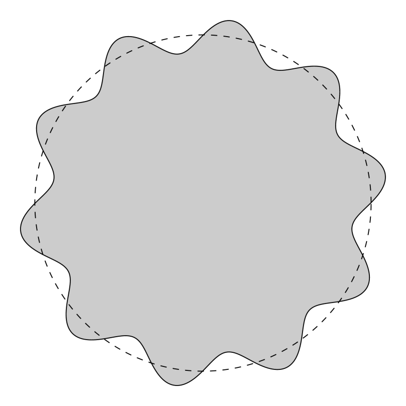
(a) $j=5$

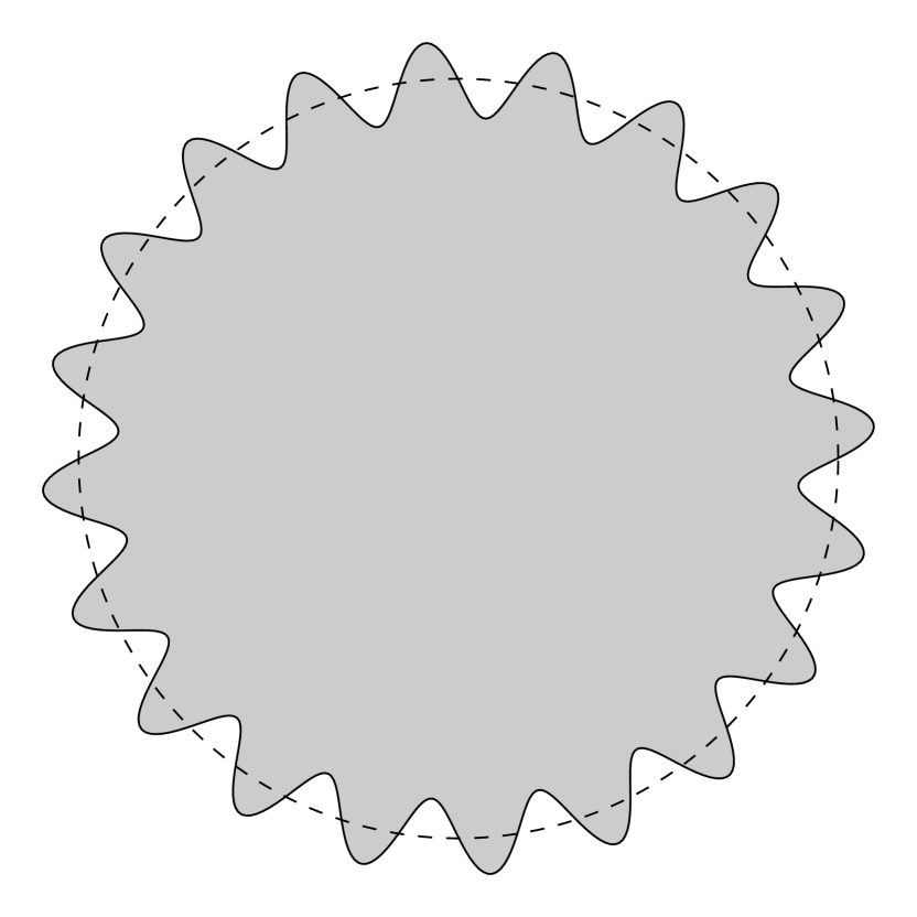
(b) $j=10$

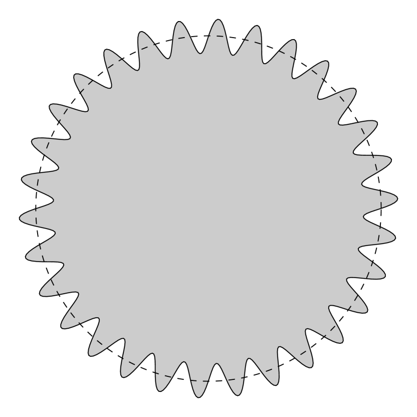
(c) $j=15$

Figure 1. The set $\Omega_{j}$, for different values of $j$, with the choice $\varepsilon=10^{-1}$. The dashed line represents the unit ball.

The volume of $\Omega_{j}$ is

$$|\Omega_{j}| =\frac{1}{2}\int_{0}^{2\pi}f^{2}_{j}({\theta})\,\textrm{d}{\theta}$$

$$=\frac{1}{2}\left(1+\frac{{\varepsilon}^{2}}{2}\right)^{-1}\int_{0}^{2\pi}1+2{\varepsilon}\sin(2j{\theta})+{\varepsilon}^{2}\sin^{2}(2j{\theta})\,\textrm{d}{\theta}$$

$$=\frac{1}{2}\left(1+\frac{{\varepsilon}^{2}}{2}\right)^{-1}(2\pi+{\varepsilon}^{2}\pi)=\pi.$$

The perimeter of $\Omega_{j}$ can be easily estimated from below as

$$P(\Omega_{j}) =\int_{0}^{2\pi}\sqrt{f^{2}_{j}({\theta})+(f^{\prime}_{j}({\theta}))^{2}}\,\textrm{d}{\theta}$$

$$=\left(1+\frac{{\varepsilon}^{2}}{2}\right)^{-\frac{1}{2}}\int_{0}^{2\pi}\sqrt{(1+{\varepsilon}\sin(2j{\theta}))^{2}+(2j{\varepsilon}\cos(2j{\theta}))^{2}}\,\textrm{d}{\theta}$$

$$\geq 2j{\varepsilon}\left(1+\frac{{\varepsilon}^{2}}{2}\right)^{-\frac{1}{2}}\int_{0}^{2\pi}|\cos(2j{\theta})|\,\textrm{d}{\theta}=8j{\varepsilon}\left(1+\frac{{\varepsilon}^{2}}{2}\right)^{-\frac{1}{2}}.$$

As we let $j\to\infty$, we see that $P(\Omega_{j})\to\infty$. Thus, all the sets $\Omega_{j}$ have the volume of the unit ball $B_{1}$, while their perimeter diverges.

Moreover, the sets $\Omega_{j}$ contain the ball $B_{\min_{\theta}f_{j}({\theta})}$, where such a radius is readily computed to be

$$\min_{\theta}f_{j}({\theta})=\left(1+\frac{{\varepsilon}^{2}}{2}\right)^{-\frac{1}{2}}(1-{\varepsilon}).$$

Therefore $h(B_{\min_{\theta}f_{j}({\theta})})$ provides an upper bound to $h(\Omega_{j})$ and $h(B_{1})=2$ a lower bound, i.e.,

$$\frac{2}{1-{\varepsilon}}\left(1+\frac{{\varepsilon}^{2}}{2}\right)^{\frac{1}{2}}\geq h(\Omega_{j})\geq 2.$$

Note that, by recalling the definition (2.3) of $\beta$, we may write $\beta^{2}(\Omega)$ as

$$P(B_{\Omega})\beta^{2}(\Omega) =\frac{1}{2}\min_{y\in{\mathbb{R}}^{n}}\int_{{\partial}^{*}\Omega}2-2\nu_{\Omega}(x)\cdot\nu_{B_{\Omega}(y)}(\pi_{y,\Omega}(x))\,\textrm{d}\mathcal{H}^{n-1}(x)$$

$$=P(\Omega)-\max_{y\in{\mathbb{R}}^{n}}\int_{{\partial}^{*}\Omega}\nu_{\Omega}(x)\cdot\frac{x-y}{|x-y|}\,\textrm{d}\mathcal{H}^{n-1}(x)$$

$$=P(\Omega)-(n-1)\,\max_{y\in{\mathbb{R}}^{n}}\int_{\Omega}\frac{\textrm{d}x}{|x-y|}$$

$$=P(\Omega)-P(B_{\Omega})+(n-1)P(B_{\Omega})\zeta(\Omega).$$

Thus, the inequality (2.12) cannot hold for all $j$ for any choice of $c(n)$, as $h(\Omega_{j})$ is uniformly bounded from above and the oscillation index

$$\beta^{2}(\Omega_{j})\geq(P(\Omega_{j})-P(B_{1}))\cdot P(B_{1})^{-1}$$

diverges as $j\to+\infty$.

Remark 2.2.

We may construct easier examples, if we do not require the competing sets to be starshaped. Consider now the family of bounded sets $\{\Omega_{j}\}_{j\in\mathbb{N}}$ with

$$\Omega_{j}:=B_{1-\frac{1}{j}}\cup A_{1,1+{\varepsilon}(j)},$$

where $A_{1,1+{\varepsilon}(j)}$ is the annulus centered at the origin with inner radius $1$ and outer radius $1+{\varepsilon}(j)$, with ${\varepsilon}(j)$ such that $|\Omega_{j}|=|B_{1}|$, for all $j$. One of these sets is depicted in Figure 2(a). It is immediate to check that $h(\Omega_{j})\to h(B_{1})$, while at the same time $\beta^{2}(\Omega_{j})\geq 2$. Thus the LHS of (2.12) goes to zero, while the RHS is uniformly strictly greater than zero. Notice that the sets of this family can be easily modified to ensure that they are all connected, see Figure 2(b).

(a) The non-connected set

(b) The connected set

Figure 2. The grayed-out sets represent one of the $\Omega_{j}$ introduced in Remark 2.2, and its connected, symmetric counterpart.

3. Estimates in the Gaussian setting

Given a set of locally finite perimeter $E\subset\mathbb{R}^{n}$, we define its Gaussian perimeter and volume to be

$$P_{\gamma}(E):=\frac{1}{(2\pi)^{\frac{n-1}{2}}}\int_{\partial^{*}E}e^{-\frac{|x|^{2}}{2}}\,\textrm{d}\mathcal{H}^{n-1}(x),\qquad\gamma(E):=\frac{1}{(2\pi)^{\frac{n}{2}}}\int_{E}e^{-\frac{|x|^{2}}{2}}\,\textrm{d}x.$$

Given any direction $\omega\in\mathbb{S}^{n-1}$ and any real number $s\in\mathbb{R}$ we denote by $H_{s,\omega}$ the halfspace $\{\,x\in\mathbb{R}^{n}:x\cdot\omega<s\,\}$. We denote by $\phi$ the function

$$\phi(s):=\frac{1}{\sqrt{2\pi}}\int_{-\infty}^{s}e^{-\frac{t^{2}}{2}}\,\textrm{d}t,$$

and have that for any direction $\omega\in\mathbb{S}^{n-1}$ it holds

$$P_{\gamma}(H_{s,\omega})=e^{-\frac{s^{2}}{2}},\qquad\gamma(H_{s,\omega})=\phi(s).$$

If the direction $\omega$ is not relevant, we shall drop it and write $H_{s}$ as a shorthand for any halfspace of measure $\phi(s)$. Moreover, given any set $E$, we denote by $H_{E}$ any halfspace such that $\gamma(E)=\gamma(H_{E})$. If the direction is relevant we denote it by $H_{E,\omega}$. The Gaussian isoperimetric inequality states that

$$P_{\gamma}(E)\geq P_{\gamma}(H_{E}),$$ (3.1)

with equality if and only if $E$ is a halfspace, see for instance [4, 9, 50]. Analogously to the Euclidean case, quantitative versions of (3.1) have been proven, namely there exists a positive constant $c=c(\gamma(E))$ depending only on the measure of $E$ (which changes from line to line) such that

$$P_{\gamma}(E)-P_{\gamma}(H_{E})\geq c\,\alpha_{\gamma}^{2}(E),$$ (3.2)

$$P_{\gamma}(E)-P_{\gamma}(H_{E})\geq c\,\beta_{\gamma}(E),$$ (3.3)

where the indexes $\alpha_{\gamma}$ and $\beta_{\gamma}$ are given by

$$\alpha_{\gamma}(E) :=\min_{\omega\in\mathbb{S}^{n-1}}|E\Delta H_{E,\omega}|,$$ (3.4)

$$\beta_{\gamma}(E) :=\min_{\omega\in\mathbb{S}^{n-1}}|b(H_{E,\omega})-b(E)|,$$ (3.5)

where $b(E)$ is the non-renormalized barycenter of $E$, i.e.,

$$b(E):=\frac{1}{(2\pi)^{\frac{n}{2}}}\int_{E}xe^{-\frac{|x|^{2}}{2}}\mathrm{d}x.$$

It is easy to see that $|b(E)|$ is maximized by the halfspace $H_{E}$, i.e., $|b(E)|\leq|b(H_{E})|$, and $s\mapsto|b(H_{s})|$ attains its maximum at $s=0$ with $|b(H_{0})|=(2\pi)^{-\frac{1}{2}}$. Moreover we note that $\beta_{\gamma}(E)\leq 1$ for every set $E$. For an account of these facts, we refer the reader to [1], where also the inequalities (3.2) and (3.3) are proven (see also [16, 18]). As in the Euclidean case the index $\beta_{\gamma}$ is stronger than $\alpha_{\gamma}$, in the sense that

$$\beta_{\gamma}(E)\gtrsim\alpha_{\gamma}^{2}(E)$$

for every measurable set $E\subset{\mathbb{R}}^{n}$.

The two following theorems are the main results of this section and they are proven respectively in Section 3.2 and Section 3.3.

Theorem 3.1.

Let $\Omega$ be an open set in ${\mathbb{R}}^{n}$. There exists a constant $c=c(\gamma(\Omega))$ such that

$$h_{\gamma}(\Omega)-h_{\gamma}(H_{\Omega})\geq c\,\alpha_{\gamma}^{2}(\Omega),$$ (3.6)

where $\alpha_{\gamma}(\cdot)$ is defined in (3.4).

Theorem 3.2.

Let $\Omega$ be an open set in ${\mathbb{R}}^{n}$. There exists a constant $c=c(\gamma(\Omega))$ such that

$$h_{\gamma}(\Omega)-h_{\gamma}(H_{\Omega})\geq c\,\frac{\beta_{\gamma}(\Omega)}{1+\sqrt{|\log(\beta_{\gamma}(\Omega))|}},$$ (3.7)

where $\beta_{\gamma}(\cdot)$ is defined in (3.5).

We remark that neither inequality (3.7) implies inequality (3.6), nor is inequality (3.6) stronger than inequality (3.7). Finally, we show in Section 3.4 by means of an example that the dependence on the asymmetry in (3.7) is optimal (see also the result in [18]).

3.1. Preliminary lemmas

In this section, we prove some lemmas regarding properties of one-dimensional functions, which are useful in the proofs of Theorems 3.1 and 3.2. We recall the definition of the complementary error function $\operatorname{erfc}(\cdot)$ and some lower and upper bounds to it, which we will use later. Given $x>0$, we set

$$\operatorname{erfc}(x):=\frac{2}{\sqrt{\pi}}\int_{x}^{+\infty}e^{t^{2}}\mathrm{d}t.$$

For $x>>1$ one has

$$\frac{e^{-x^{2}}}{\sqrt{\pi}}\left(\frac{1}{x}-\frac{1}{x^{3}}\right)\leq\operatorname{erfc}(x)\leq\frac{e^{-x^{2}}}{\sqrt{\pi}}\left(\frac{1}{x}\right)$$ (3.8)

as one can easily infer by using the asymptotic expansion of the complementary error function.

Lemma 3.3.

Let $\varphi\colon{\mathbb{R}}\to(0,\infty)$ be the function defined as

$$\varphi(s):=\frac{P_{\gamma}(H_{s})}{\gamma(H_{s})}.$$

Then, $\varphi^{\prime}(s)<0$ for all $s\in\mathbb{R}$, and $\lim_{s\to-\infty}\varphi(s)=+\infty$.

Proof.

The first part of the claim is equivalent to show that the function $f(s)=\sqrt{2\pi}(\varphi(s))^{-1}$ satisfies $f^{\prime}(s)>0$ for all $s\in{\mathbb{R}}$. Using the definition of the Gaussian perimeter and volume, we may equivalently write

$$f(s)=\sqrt{2\pi}\,e^{\frac{s^{2}}{2}}\phi(s).$$

As $\sqrt{2\pi}\,\phi^{\prime}(s)=e^{-\frac{s^{2}}{2}}$, one readily computes the first derivative of $f$

$$f^{\prime}(s)=1+sf(s)=1+se^{\frac{s^{2}}{2}}\sqrt{2\pi}\phi(s),$$ (3.9)

which in particular is continuous. Trivially, $f^{\prime}(s)\geq 1$ for $s\geq 0$. Thus we are left to check that $f^{\prime}(s)>0$, for values $s<0$.

By integration by parts we have

$$\sqrt{2\pi}\phi(s)=\int_{-\infty}^{s}\left(-\frac{1}{t}\right)(-te^{-\frac{t^{2}}{2}})\,\textrm{d}t=-\frac{e^{-\frac{s^{2}}{2}}}{s}-\int_{-\infty}^{s}\frac{1}{t^{2}}e^{-\frac{t^{2}}{2}}\,\textrm{d}t,$$

which plugged in (3.9) yields

$$f^{\prime}(s)=-se^{\frac{s^{2}}{2}}\int_{-\infty}^{s}\frac{1}{t^{2}}e^{-\frac{t^{2}}{2}}\,\textrm{d}t.$$

It is immediate that, for any fixed $s<0$, this is positive. Hence, we have the first part of the claim.

To check the second part, we use the upper bound on $\operatorname{erfc}$ given in (3.8). For $s<<-1$, we have

$$\frac{1}{\sqrt{2\pi}}\varphi(s)=\frac{e^{-\frac{s^{2}}{2}}}{\int_{-\infty}^{s}e^{-\frac{t^{2}}{2}}\textrm{d}t}=\frac{e^{-\frac{s^{2}}{2}}}{\int_{|s|}^{+\infty}e^{-\frac{t^{2}}{2}}\textrm{d}t}=\frac{e^{-\frac{s^{2}}{2}}}{\sqrt{\frac{\pi}{2}}\operatorname{erfc}\left(\frac{|s|}{\sqrt{2}}\right)}\geq|s|,$$

which completes the proof. ∎

For the sake of completeness, we remark two consequences of Lemma 3.3. First, Gaussian Cheeger sets exist. Second, the Cheeger set of any given halfspace $H_{s}$ is the halfspace itself. Indeed, when proving existence one easily sees that any minimizing sequence $\{E_{k}\}_{k}$ is bounded in $BV_{\gamma}({\mathbb{R}}^{n})$ and hence, up to a subsequence, it converges to some set $E$. By the lower semicontinuity of $P_{\gamma}(\cdot)$, in order to show that this limit set is a minimizer one only needs to check that $\gamma(E)>0$. The previous lemma can be used to show that minimizing sequences are such that $\gamma(E_{k})$ does not converge to $0$, as the ratio $P_{\gamma}(E_{k})\gamma(E_{k})^{-1}$ would otherwise be unbounded. Regarding the minimality of $H_{s}$, the Gaussian isoperimetric inequality ensures that for any fixed volume the halfspace is the perimeter minimizer, while the lemma ensures that any halfspace $H_{\sigma}$ strictly contained in $H_{s}$ has ratio $P_{\gamma}(H_{\sigma})\gamma(H_{\sigma})^{-1}$ bigger than that of $H_{s}$.

Lemma 3.4.

Let $\Phi:[0,1]\to[0,1]$ be the function

$$\Phi(\rho)=\frac{\rho}{1+\sqrt{|\log(\rho)|}},$$ (3.10)

defined by continuity at $\rho=0$ as $\Phi(0)=0$. Then, $\Phi$ is increasing, with

$$\Phi(\rho)\leq\rho$$ (3.11)

and

$$\Phi\left(\frac{1}{4}\rho\right)\geq\frac{1}{4(1+\sqrt{\log(4)})}\Phi(\rho).$$ (3.12)

Proof.

We begin by showing that $\Phi$ is increasing. We have

$$\Phi^{\prime}(\rho)=\frac{1}{1+\sqrt{|\log(\rho)|}}-\frac{\operatorname{sgn}(\log(\rho))}{2\sqrt{|\log(\rho)|}(1+\sqrt{|\log(\rho)|})^{2}}.$$

Since $\rho\in[0,1]$, we immediately get $\Phi^{\prime}(\rho)\geq 0$ as $\operatorname{sgn}(\log(\rho))\leq 0$. Also the bound (3.11) is trivial.

We are left with (3.12). To this aim we write

$$\Phi(\rho/4)=\frac{\rho/4}{1+\sqrt{|\log(\rho/4)|}}=\frac{1}{4}\Phi(\rho)\frac{1+\sqrt{|\log(\rho)|}}{1+\sqrt{|\log(\rho/4)|}}.$$

The claim follows as

$$g(\rho):=\frac{1+\sqrt{|\log(\rho)|}}{1+\sqrt{|\log(\rho/4)|}}$$

attains its minimum over the interval $[0,1]$ at $\rho=1$. Indeed, one can check that $g(\rho)$ is decreasing in $[0,1]$. ∎

Thanks to the monotonicity property stated in the above lemma, we can now show that we can control from above $\Phi(|b(E)|)$ with the mass of the set itself $\gamma(E)$, up to some multiplicative, universal constant.

Lemma 3.5.

There is a constant $C$ such that for any set $E\subset{\mathbb{R}}^{n}$ it holds

$$\Phi(|b(E)|)\leq C\gamma(E).$$

Proof.

First recall that for any set $E$ it holds $|b(E)|\leq|b(H_{E})|$. Therefore, by the monotonicity of $\Phi$ we have

$$\Phi(|b(E)|)\leq\Phi(|b(H_{E})|).$$

Hence, to prove the claim it suffices to show the validity of the inequality for halfspaces. Second, as $\Phi(|b(E)|)\leq 1$, it is enough to prove the inequality for small values of $\gamma(H_{E})$, and thus of $|b(H_{E})|$.

We denote by $s_{E}:=\phi^{-1}(\gamma(H_{E}))$. To conclude we need to prove the inequality

$$\Phi(|b(H_{E})|)\leq C\gamma(H_{E}),$$

for values $s_{E}<0$ such that $|s_{E}|>>1$. First, notice that

$$\gamma(H_{E})=\frac{1}{\sqrt{2\pi}}\int_{-\infty}^{s_{E}}e^{-\frac{t^{2}}{2}}\,\textrm{d}t, |b(H_{E})|=\frac{1}{\sqrt{2\pi}}e^{-\frac{s_{E}^{2}}{2}}.$$

On the one hand, for all $s$ we have

$$\begin{split}\Phi(|b(H_{s})|)&=\Phi\left(\frac{1}{\sqrt{2\pi}}e^{-\frac{s^{2}}{2}}\right)=\frac{e^{-\frac{s^{2}}{2}}}{\sqrt{2\pi}\left(1+\sqrt{\left|\log((2\pi)^{-\frac{1}{2}}e^{-\frac{s^{2}}{2}})\right|}\right)}\\ &=\frac{e^{-\frac{s^{2}}{2}}}{\sqrt{2\pi}\left(1+\sqrt{\frac{1}{2}\log(2\pi)+\frac{|s|^{2}}{2}}\right)}\leq\frac{e^{-\frac{s^{2}}{2}}}{\sqrt{2\pi}\left(1+\frac{|s|}{\sqrt{2}}\right)}.\end{split}$$ (3.13)

On the other hand, for $s<0$ such that $|s|>>1$, using the asymptotic behavior of $\operatorname{erfc}$ given in (3.8), we have

$$\begin{split}\gamma(H_{s})&=\phi(s)=\frac{1}{\sqrt{2\pi}}\int_{-\infty}^{s}e^{-\frac{t^{2}}{2}}\textrm{d}t=\frac{1}{\sqrt{2\pi}}\int_{|s|}^{+\infty}e^{-\frac{t^{2}}{2}}\textrm{d}t\\ &=\frac{1}{\sqrt{2\pi}}\sqrt{\frac{\pi}{2}}\operatorname{erfc}\left(\frac{|s|}{\sqrt{2}}\right)\geq\frac{e^{-\frac{|s|^{2}}{2}}}{\sqrt{2\pi}}\left(\frac{1}{|s|}-\frac{2}{|s|^{3}}\right)\end{split}$$ (3.14)

Using (3.13) and (3.14) the claim boils down to check that there exists a constant $C>0$ such that the inequality

$$C\left(1+\frac{|s|}{\sqrt{2}}\right)\geq\frac{|s|^{3}}{|s|^{2}-2},$$

holds for values $|s|>>1$. This is obviously true for $C\geq\sqrt{2}$. ∎

3.2. Proof of Theorem 3.1

Let $E\subset\Omega$ be a Cheeger set of $\Omega$. Then

$$h_{\gamma}(\Omega)-h_{\gamma}(H_{\Omega})=\frac{P_{\gamma}(E)-P_{\gamma}(H_{E})}{\gamma(E)}+\left(\frac{P_{\gamma}(H_{E})}{\gamma(E)}-\frac{P_{\gamma}(H_{\Omega})}{\gamma(\Omega)}\right).$$ (3.15)

Let us first show that we may assume that

$${\varepsilon}\leq\gamma(E)\leq 1-{\varepsilon},$$ (3.16)

for ${\varepsilon}>0$ which depends on $\gamma(\Omega)$. The upper bound in (3.16) follows simply from $E\subset\Omega$ and thus $\gamma(E)\leq\gamma(\Omega)\leq 1-{\varepsilon}_{1}$. Here ${\varepsilon}_{1}=1-\gamma(\Omega)>0$ as we may obviously assume that $\Omega\neq{\mathbb{R}}^{n}$. For the lower bound, we first notice that $\alpha_{\gamma}(\Omega)\leq 2\gamma(\Omega)$, and thus (3.6) immediately follows if $h_{\gamma}(\Omega)-h_{\gamma}(H_{\Omega})\geq 2$, by choosing $c(\gamma(\Omega))\leq\gamma(\Omega)^{-1}$. Hence, we may assume $h_{\gamma}(\Omega)-h_{\gamma}(H_{\Omega})<2$. Let us set $s_{\Omega}:=\phi^{-1}(\gamma(\Omega))$ and $s_{E}:=\phi^{-1}(\gamma(E))$. Clearly, $s_{E}<s_{\Omega}$. Then, we have

$$\varphi(s_{E})-\varphi(s_{\Omega})=\frac{P_{\gamma}(H_{E})}{\gamma(E)}-\frac{P_{\gamma}(H_{\Omega})}{\gamma(\Omega)}=h_{\gamma}(\Omega)-h_{\gamma}(H_{\Omega})<2.$$

The behavior of $\varphi(s)\to\infty$ as $s\to-\infty$ given in Lemma 3.3 implies that $\gamma(E)>{\varepsilon}_{2}={\varepsilon}_{2}(\gamma(\Omega))$. Setting ${\varepsilon}:=\min\{{\varepsilon}_{1},{\varepsilon}_{2}\}$ we obtain (3.16). In particular, there exists $R=R(\gamma(\Omega))$ such that $-R\leq s_{E}\leq s_{\Omega}\leq R$.

By the quantitative isoperimetric inequality (3.2) we have

$$\frac{P_{\gamma}(E)-P_{\gamma}(H_{E})}{\gamma(E)}\geq\frac{1}{\gamma(E)}c(s_{E})\alpha_{\gamma}^{2}(E),$$ (3.17)

where $c(s_{E})=\frac{1}{\kappa}(1+s_{E}^{2})^{-1}e^{\frac{s_{E}^{2}}{2}}$ with $\kappa>0$ a universal constant, as can be seen in [1]. As $s_{E}\in[-R,R]$ we may replace $\gamma(E)^{-1}c(s_{E})$ with a constant $c=c(R)$, thus ultimately with $c_{1}=c_{1}(\gamma(\Omega))$.

On the other hand, Lemma 3.3 coupled with the fact that $(\phi^{-1})^{\prime}>0$ and two subsequent applications of the Mean Value Theorem imply

$$\begin{split}\frac{P_{\gamma}(H_{E})}{\gamma(E)}-&\frac{P_{\gamma}(H_{\Omega})}{\gamma(\Omega)}=-\varphi^{\prime}(\xi)(s_{\Omega}-s_{E})\geq\tilde{c}_{2}(s_{\Omega}-s_{E})\\ &\geq\tilde{c}_{2}(\phi^{-1})^{\prime}(\hat{\xi})(\gamma(\Omega)-\gamma(E))\geq c_{2}(\gamma(\Omega)-\gamma(E)),\end{split}$$ (3.18)

where the two constants can be chosen as $\tilde{c}_{2}=\min_{[-R,R]}\{-\varphi^{\prime}(s)\}$, and $c_{2}=\tilde{c}_{2}\,\min_{[{\varepsilon},1-{\varepsilon}]}\{(\phi^{-1})^{\prime}(\rho)\}$, and thus they ultimately depend only on $\gamma(\Omega)$. Combining the inequalities (3.15), (3.17) and (3.18) yields

$$h_{\gamma}(\Omega)-h_{\gamma}(H_{\Omega}) \geq c_{1}\alpha_{\gamma}^{2}(E)+c_{2}(\gamma(\Omega)-\gamma(E))$$

$$\geq\frac{1}{5}\min\{c_{1},c_{2}\}(\alpha_{\gamma}(E)+\gamma(\Omega)-\gamma(E))^{2}$$

$$\geq c\,(\gamma(\Omega))(\alpha_{\gamma}(E)+\gamma(\Omega)-\gamma(E))^{2},$$ (3.19)

where we used that $\gamma(\Omega)-\gamma(E)\leq 1$ and $\alpha_{\gamma}(E)\leq 2$.

We now set $H_{E}$ to be the halfspace with the same measure as $E$ such that $\alpha_{\gamma}(E)=\gamma(E\Delta H_{E})$, and $H_{\Omega}$ to be the halfspace with the same measure as $\Omega$ containing $H_{E}$. Then, we have

$$\alpha_{\gamma}(E)=\gamma(E\Delta H_{E})\geq\gamma(E\setminus H_{E})=\gamma(E)-\gamma(E\cap H_{E}).$$

Using the inequality above, that $E\subset\Omega$, that $H_{E}\subset H_{\Omega}$ and the equality $2\gamma(\Omega\setminus H_{\Omega})=\gamma(\Omega\Delta H_{\Omega})$ we get the following estimate

$$(\alpha_{\gamma}(E) +\gamma(\Omega)-\gamma(E))^{2}\geq(\gamma(\Omega)-\gamma(E\cap H_{E}))^{2}$$

$$\geq(\gamma(\Omega)-\gamma(\Omega\cap H_{E}))^{2}=\gamma(\Omega\setminus H_{E})^{2}$$

$$\geq\gamma(\Omega\setminus H_{\Omega})^{2}=\frac{1}{4}\gamma(\Omega\Delta H_{\Omega})^{2}\geq\frac{1}{4}\alpha_{\gamma}^{2}(\Omega).$$ (3.20)

Inequality (3.19) paired with (3.20) finally yields the claim.

3.3. Proof of Theorem 3.2

Recall that $\beta_{\gamma}(\Omega)\leq 1$, and recall the definition of $\Phi(\rho)$ given in (3.10). Thus, we aim to show

$$h_{\gamma}(\Omega)-h_{\gamma}(H_{\Omega})\geq c\,\Phi(\beta_{\gamma}(\Omega)).$$

We begin by noticing that

$$\beta_{\gamma}(\Omega)=|b(H_{\Omega})-b(\Omega)|\leq 4|b(H_{\Omega})|.$$

Hence, by the properties of the function $\Phi$ established in Lemma 3.4, together with Lemma 3.5, we have

$$\Phi(\beta_{\gamma}(\Omega))\leq C\gamma(\Omega).$$

Thus, as in the proof of Theorem 3.1 we may assume without loss of generality that $h_{\gamma}(\Omega)-h_{\gamma}(H_{\Omega})<C$, since otherwise the claim follows as before. Then, we may argue again as in the proof of Theorem 3.1 and we may assume without loss of generality

$${\varepsilon}\leq\gamma(E)\leq 1-{\varepsilon},$$

for ${\varepsilon}>0$ which depends only on $\gamma(\Omega)$, because otherwise the claim immediately follows. Then, we may argue again as in the proof of Theorem 3.1 and obtain inequality (3.18). In place of using the quantitative isoperimetric inequality (3.2) and obtaining (3.17) we use the strong quantitative isoperimetric inequality (3.3) and get

$$\frac{P_{\gamma}(E)-P_{\gamma}(H_{E})}{\gamma(E)}\geq\frac{1}{\gamma(E)}c(s_{E})\beta_{\gamma}(E),$$ (3.21)

now with $c(s_{E})=\frac{1}{\kappa}(1+s_{E}^{2})^{-1}$ (see again [1]), and thus ultimately a constant $c_{1}=c_{1}(\gamma(\Omega))$.

Combining (3.15) with (3.21) and (3.18) we deduce

$$h_{\gamma}(\Omega)-h_{\gamma}(H_{\Omega})\geq c_{1}\beta_{\gamma}(E)+c_{2}\,(\gamma(\Omega)-\gamma(E)).$$ (3.22)

We fix $H_{E}$ to be the halfspace such that $\beta_{\gamma}(E)=|b(H_{E})-b(E)|$, and we let $H_{\Omega}$ be the halfspace with the same measure of $\Omega$ such that $H_{E}\subset H_{\Omega}$. By splitting $H_{\Omega}$ into $H_{E}$ and $H_{\Omega}\setminus H_{E}$, adding and removing $b(E)$, and using the triangle inequality, we get

$$\beta_{\gamma}(\Omega)\leq|b(H_{\Omega})-b(\Omega)| =|b(H_{E})-b(E)+b(H_{\Omega}\setminus H_{E})+b(E)-b(\Omega)|$$

$$\leq\beta_{\gamma}(E)+|b(H_{\Omega}\setminus H_{E})|+|b(E)-b(\Omega)|$$

$$=\beta_{\gamma}(E)+|b(H_{\Omega}\setminus H_{E})|+|b(\Omega\setminus E)|$$

$$\leq 2\max\{\beta_{\gamma}(E),|b(H_{\Omega}\setminus H_{E})|+|b(\Omega\setminus E)|\}.$$

Thus we have either

$$\beta_{\gamma}(\Omega)\leq 2\beta_{\gamma}(E),$$ (3.23)

or

$$\beta_{\gamma}(\Omega)\leq 2\big{(}|b(H_{\Omega}\setminus H_{E})|+|b(\Omega\setminus E)|\big{)}.$$ (3.24)

If (3.23) holds true, we obtain the result by (3.11), (3.23) and (3.22). If (3.24) holds true, we have that

$$\frac{1}{4}\beta_{\gamma}(\Omega)\leq\max\{|b(H_{\Omega}\setminus H_{E})|,|b(\Omega\setminus E)|\}.$$

By the monotonicity of $\Phi$ and its property (3.12), it follows

$$\Phi(\beta_{\gamma}(\Omega))\leq 4(1+\sqrt{\log(4)})\max\{\Phi(|b(H_{\Omega}\setminus H_{E})|),\Phi(|b(\Omega\setminus E)|)\}.$$

As the sets $H_{\Omega}\setminus H_{E}$ and $\Omega\setminus E$ have the same Gaussian measure, and as $E\subset\Omega$, by Lemma 3.5 we finally get

$$\Phi(\beta_{\gamma}(\Omega))\leq C(\gamma(\Omega\setminus E))=C(\gamma(\Omega)-\gamma(E)),$$

which coupled with (3.22) allows us to conclude.

3.4. The sharpness of the inequality with the index $\beta_{\gamma}$

In this section, we show that the dependence on the asymmetry in Theorem 3.2 is sharp. Let $T>>1$, and let us define the family of one-dimensional sets $\{\Omega_{T}\}_{T}$ as

$$\Omega_{T}:=(-\infty,-1)\cup(T,+\infty).$$

(a) The one-dimensional set $\Omega_{T}$

(b) The halfline $H_{\Omega_{T}}$

Figure 3. The set $\Omega_{T}$ and the corresponding halfline $H_{\Omega_{T}}$.

It is easy to notice, that for $T>1$ the Cheeger set of $\Omega$ is given by the halfline $(-\infty,-1)$. The halfline of same volume of $\Omega$ is

$$H_{\Omega_{T}}=(-\infty,-1+{\varepsilon}(T)),$$

where ${\varepsilon}(T)$ is such that

$$\int_{T}^{+\infty}e^{-\frac{t^{2}}{2}}\mathrm{d}t=\int_{-1}^{-1+{\varepsilon}(T)}e^{-\frac{t^{2}}{2}}\mathrm{d}t,$$ (3.25)

and obviously ${\varepsilon}(T)\to 0$, as $T\to+\infty$. For the convenience of the reader, $\Omega_{T}$ is depicted in Figure 3(a), while the corresponding halfline $H_{\Omega_{T}}$ in Figure 3(b). By recalling the definition of the function $\varphi$ in Lemma 3.3, we have by the Mean Value Theorem

$$h_{\gamma}(\Omega)-h_{\gamma}(H_{\Omega})=\frac{P_{\gamma}((-\infty,-1))}{\gamma((-\infty,-1))}-\frac{P_{\gamma}((-\infty,-1+{\varepsilon}(T)))}{\gamma((-\infty,-1+{\varepsilon}(T)))}=-\varphi^{\prime}(\xi){\varepsilon}(T),$$

for some $\xi\in(-1,-1+{\varepsilon}(T))$. Hence, we immediately obtain the upper bound

$$h_{\gamma}(\Omega)-h_{\gamma}(H_{\Omega})\leq C\,{\varepsilon}(T),$$ (3.26)

by choosing $T>>1$ in such a way that ${\varepsilon}(T)<1$ and $C=\min_{[-1,0]}\{-\varphi^{\prime}(x)\}$ independent of ${\varepsilon}$. We now aim to bound $\beta_{\gamma}(\Omega)$ from below and show that

$$\frac{\beta_{\gamma}(\Omega)}{1+\sqrt{|\log(\beta_{\gamma}(\Omega))|}}\geq c\,{\varepsilon}(T).$$ (3.27)

This inequality and inequality (3.26) immediately show that Theorem 3.2 is sharp. Let us prove inequality (3.27).

By definition of $\beta_{\gamma}(\Omega)$, we have

$$\beta_{\gamma}(\Omega)=|b(H_{\Omega})-b(\Omega)|=\frac{1}{\sqrt{2\pi}}\left(e^{-\frac{({\varepsilon}(T)-1)^{2}}{2}}-e^{-\frac{1}{2}}+e^{-\frac{T^{2}}{2}}\right).$$ (3.28)

We now use (3.25) to bound this quantity from below as follows. On the one hand, for the LHS of (3.25), one has

$$\int_{T}^{+\infty}e^{-\frac{t^{2}}{2}}\mathrm{d}t=\sqrt{2}\int_{\frac{T}{\sqrt{2}}}^{+\infty}e^{-x^{2}}\mathrm{d}x=\sqrt{\frac{\pi}{2}}\operatorname{erfc}\left(\frac{T}{\sqrt{2}}\right)\leq\frac{1}{T}e^{-\frac{T^{2}}{2}},$$

where we used the asymptotic behavior of $\operatorname{erfc}$ given in (3.8). On the other hand, for the RHS of (3.25), one has

$$\int_{-1}^{-1+{\varepsilon}(T)}e^{-\frac{t^{2}}{2}}\mathrm{d}t\geq\int_{-1}^{-1+{\varepsilon}(T)}-te^{-\frac{t^{2}}{2}}\mathrm{d}t=e^{-\frac{t^{2}}{2}}\Big{|}_{-1}^{-1+{\varepsilon}(T)}=e^{-\frac{({\varepsilon}(T)-1)^{2}}{2}}-e^{-\frac{1}{2}}.$$

Combining these two inequalities, we get

$$e^{-\frac{T^{2}}{2}}\geq T\left(e^{-\frac{({\varepsilon}(T)-1)^{2}}{2}}-e^{-\frac{1}{2}}\right).$$ (3.29)

Thus by (3.28) and (3.29) we get

$$\beta_{\gamma}(\Omega)\geq\frac{1}{\sqrt{2\pi}}(1+T)\left(e^{-\frac{({\varepsilon}(T)-1)^{2}}{2}}-e^{-\frac{1}{2}}\right)\geq c\,(1+T)\,{\varepsilon}(T).$$ (3.30)

By using again the asymptotic behavior of $\operatorname{erfc}$ given in (3.8) we may estimate the LHS of (3.25) as

$$\int_{T}^{+\infty}e^{-\frac{t^{2}}{2}}\mathrm{d}t\geq\frac{1}{2T}e^{-\frac{T^{2}}{2}},$$

and we simply estimate the RHS of (3.25) as

$$\int_{-1}^{-1+{\varepsilon}(T)}e^{-\frac{t^{2}}{2}}\mathrm{d}t\leq 2\int_{-1}^{-1+{\varepsilon}(T)}-te^{-\frac{t^{2}}{2}}\mathrm{d}t=2\left(e^{-\frac{({\varepsilon}(T)-1)^{2}}{2}}-e^{-\frac{1}{2}}\right)$$

for $T>>1$. Hence, we deduce by (3.25)

$$e^{-\frac{T^{2}}{2}}\leq 4T\left(e^{-\frac{({\varepsilon}(T)-1)^{2}}{2}}-e^{-\frac{1}{2}}\right)\leq c\,T\,{\varepsilon}(T)$$

for $T>>1$. Combining this last inequality with inequality (3.30) yields

$$\beta_{\gamma}(\Omega)\geq c(1+T){\varepsilon}(T)\geq cT{\varepsilon}(T)\geq c\,e^{-\frac{T^{2}}{2}}\geq e^{-T^{2}},$$ (3.31)

for T big enough. Recalling that $\beta_{\gamma}(\Omega)<1$ for $T>>1$ by (3.31) we get

$$\sqrt{|\log(\beta_{\gamma}(\Omega))|}\leq T,$$

for $T$ big enough. This and inequality (3.30) imply the inequality (3.27).

Counterexamples in higher dimensions can be constructed in the same exact way. Notice that in higher dimensions, one can as well provide P-connected counterexamples, by adding a suitably thin tube connecting the two halfspaces defining $\Omega_{T}$.

References

- [1] M. Barchiesi, A. Brancolini, and V. Julin. Sharp dimension free quantitative estimates for the Gaussian isoperimetric inequality. Ann. Prob., 45(2):668–697, 2017. doi:10.1214/15-AOP1072.
- [2] M. Barchiesi and V. Julin. Robustness of the Gaussian concentration inequality and the Brunn–Minkowski inequality. Calc. Var. Partial Differential Equations, 56(3):80, 2017. doi:10.1007/s00526-017-1169-x.
- [3] V. Bobkov and E. Parini. On the Cheeger problem for rotationally invariant domains. Manuscripta Math., Ahead of print. doi:10.1007/s00229-020-01260-9.
- [4] C. Borell. The Brunn–Minkowski inequality in Gauss space. Invent. Math., 30(2):207–216, 1975. doi:10.1007/BF01425510.
- [5] L. Brasco and G. De Philippis. Spectral inequalities in quantitative form. In A. Henrot, editor, Shape Optimization and Spectral Theory, chapter 7, pages 201–281. De Gruyter Open, Warsaw, 2017. doi:10.1515/9783110550887-007.
- [6] L. Brasco, G. De Philippis, and B. Velichkov. Faber–Krahn inequalities in sharp quantitative form. Duke Math. J., 164(9):1777–1831, 2015. doi:10.1215/00127094-3120167.
- [7] L. Brasco, E. Lindgren, and E. Parini. The fractional Cheeger problem. Interfaces Free Bound., 16(3):419–458, 2014. doi:10.4171/IFB/325.
- [8] H. Bueno and G. Ercole. Solutions of the Cheeger problem via torsion functions. J. Math. Anal. Appl., 381(1):263–279, 2011. doi:10.1016/j.jmaa.2011.03.002.
- [9] E. A. Carlen and C. Kerce. On the cases of equality in Bobkov’s inequality and Gaussian rearrangement. Calc. Var. Partial Differential Equations, 13:1–18, 2001. doi:10.1007/PL00009921.
- [10] V. Caselles, G. Facciolo, and E. Meinhardt. Anisotropic Cheeger sets and applications. SIAM J. Imaging Sciences, 2(4):1211–1254, 2009. doi:10.1137/08073696X.
- [11] V. Caselles, M. Jr. Miranda, and M. Novaga. Total variation and Cheeger sets in Gauss space. J. Funct. Anal., 259(6):1491–1516, 2010. doi:10.1016/j.jfa.2010.05.007.
- [12] J. Cheeger. A lower bound for the smallest eigenvalue of the Laplacian. In Problems in analysis (Papers dedicated to Salomon Bochner, 1969), pages 195–199. Princeton Univ. Press, Princeton, N. J., 1970.
- [13] A. Cianchi. A quantitative Sobolev inequality in . J. Funct. Anal., 237(2):466–481, 2006. doi:10.1016/j.jfa.2005.12.008.
- [14] A. Cianchi. Sharp Sobolev–Morrey inequalities and the distance from extremals. Trans. Amer. Math. Soc., 360(8):4335–4347, 2008. doi:10.1090/S0002-9947-08-04491-7.
- [15] A. Cianchi, N. Fusco, F. Maggi, and A. Pratelli. The sharp Sobolev inequality in quantitative form. J. Eur. Math. Soc. (JEMS), 11(5):1105–1139, 2009. doi:10.4171/JEMS/176.
- [16] A. Cianchi, N. Fusco, F. Maggi, and A. Pratelli. On the isoperimetric deficit in Gauss space. Amer. J. Math., 133(1):131–186, 2011. doi:10.1353/ajm.2011.0005.
- [17] F. Demengel. Functions locally almost -harmonic. Appl. Anal., 83(9):865–896, 2004. doi:10.1080/00036810310001621369.
- [18] R. Eldan. A two-sided estimate for the Gaussian noise stability deficit. Invent. Math., 201(2):561–624, 2015. doi:10.1007/s00222-014-0556-6.
- [19] L. Esposito, N. Fusco, and C. Trombetti. A quantitative version of the isoperimetric inequality: the anisotropic case. Ann. Scuola Norm. Sup. Pisa Cl. Sci. (5), 4(4):619–651, 2005. URL: http://www.numdam.org/item/ASNSP_2005_5_4_4_619_0/.
- [20] A. Figalli, F. Maggi, and A. Pratelli. A note on Cheeger sets. Proc. Amer. Math. Soc., 137(6):2057–2062, 2009. doi:10.1090/S0002-9939-09-09795-0.
- [21] A. Figalli, F. Maggi, and A. Pratelli. A mass transportation approach to quantitative isoperimetric inequalities. Invent. Math., 182(1):167–211, 2010. doi:10.1007/s00222-010-0261-z.
- [22] L. E. Fraenkel. On the increase of capacity with asymmetry. Comput. Methods Funct. Theory, 8(1-2):203–224, 2008. doi:10.1007/BF03321684.
- [23] R. L. Frank and E. H. Lieb. A note on a theorem of M. Christ. arXiv:1909.04598.
- [24] B. Fuglede. Stability in the isoperimetric problem for convex or nearly spherical domains in . Trans. Amer. Math. Soc., 314(2):619–638, 1989. doi:10.2307/2001401.
- [25] N. Fusco. The quantitative isoperimetric inequality and related topics. Bull. Math. Sci., 5(3):517–607, 2015. doi:10.1007/s13373-015-0074-x.
- [26] N. Fusco and V. Julin. A strong form of the quantitative isoperimetric inequality. Calc. Var. Partial Differential Equations, 50(3-4):925–937, 2014. doi:10.1007/s00526-013-0661-1.
- [27] N. Fusco, F. Maggi, and A. Pratelli. The sharp quantitative Sobolev inequality for functions of bounded variation. J. Funct. Anal., 244(1):315–341, 2007. doi:10.1016/j.jfa.2006.10.015.
- [28] N. Fusco, F. Maggi, and A. Pratelli. The sharp quantitative isoperimetric inequality. Ann. of Math. (2), 168(3):941–980, 2008. doi:10.4007/annals.2008.168.941.
- [29] N. Fusco, F. Maggi, and A. Pratelli. Stability estimates for certain Faber–Krahn, isocapacitary and Cheeger inequalities. Ann. Scuola Norm. Sup. Pisa Cl. Sci. (5), 8(1):51–71, 2009. URL: http://www.numdam.org/item/ASNSP_2009_5_8_1_51_0/.
- [30] N. Fusco and A. Pratelli. Sharp stability for the Riesz potential. ESAIM Control Optim. Calc. Var., 26:113, 2020. doi:10.1051/cocv/2020024.
- [31] E. Giusti. On the equation of surfaces of prescribed mean curvature. Existence and uniqueness without boundary conditions. Invent. Math., 46(2):111–137, 1978. doi:10.1007/BF01393250.
- [32] W. Hansen and N. Nadirashvili. Isoperimetric inequalities in potential theory. Potential Anal., 3(1):1–14, 1994. doi:10.1007/BF01047833.
- [33] I. R. Ionescu and T. Lachand-Robert. Generalized Cheeger sets related to landslides. Calc. Var. Partial Differential Equations, 23(2):227–249, 2005. doi:10.1007/s00526-004-0300-y.
- [34] V. Julin. Isoperimetric problem with a Coulomb repulsive term. Indiana Univ. Math. J., 63(1):77–89, 2014. doi:10.1512/iumj.2014.63.5185.
- [35] B. Kawohl and V. Fridman. Isoperimetric estimates for the first eigenvalue of the -Laplace operator and the Cheeger constant. Comment. Math. Univ. Carolin., 44(4):659–667, 2003.
- [36] B. Kawohl and T. Lachand-Robert. Characterization of Cheeger sets for convex subsets of the plane. Pacific J. Math., 225(1):103–118, 2006. doi:10.2140/pjm.2006.225.103.
- [37] D. Krejčiřík, G. P. Leonardi, and P. Vlachopulos. The Cheeger constant of curved tubes. Arch. Math. (Basel), 112(4):429–436, 2019. doi:10.1007/s00013-018-1282-x.
- [38] G. P. Leonardi. An overview on the Cheeger problem. In New Trends in Shape Optimization, volume 166 of Internat. Ser. Numer. Math., pages 117–139. Springer Int. Publ., 2015. doi:10.1007/978-3-319-17563-8_6.
- [39] G. P. Leonardi, R. Neumayer, and G. Saracco. The Cheeger constant of a Jordan domain without necks. Calc. Var. Partial Differential Equations, 56(6):164, 2017. doi:10.1007/s00526-017-1263-0.
- [40] G. P. Leonardi and A. Pratelli. On the Cheeger sets in strips and non-convex domains. Calc. Var. Partial Differential Equations, 55(1):15, 2016. doi:10.1007/s00526-016-0953-3.
- [41] G. P. Leonardi and G. Saracco. The prescribed mean curvature equation in weakly regular domains. NoDEA Nonlinear Differ. Equ. Appl., 25(2):9, 2018. doi:10.1007/s00030-018-0500-3.
- [42] G. P. Leonardi and G. Saracco. Minimizers of the prescribed curvature functional in a Jordan domain with no necks. ESAIM Control Optim. Calc. Var., 26:76, 2020. doi:10.1051/cocv/2020030.
- [43] Q. Li and M. Torres. Morrey spaces and generalized Cheeger sets. Adv. Calc. Var., 12(2):111–133, 2019. doi:10.1515/acv-2016-0050.
- [44] R. Neumayer. A strong form of the quantitative Wulff inequality. SIAM J. Math. Anal., 48(3):1727–1772, 2016. doi:10.1137/15M1013675.
- [45] R. Neumayer. A note on strong-form stability for the Sobolev inequality. Calc. Var. Partial Differential Equations, 59(1):25, 2020. doi:10.1007/s00526-019-1686-x.
- [46] E. Parini. An introduction to the Cheeger problem. Surv. Math. Appl., 6:9–21, 2011.
- [47] A. Pratelli and G. Saracco. On the generalized Cheeger problem and an application to 2d strips. Rev. Mat. Iberoam., 33(1):219–237, 2017. doi:10.4171/RMI/934.
- [48] G. Saracco. Weighted Cheeger sets are domains of isoperimetry. Manuscripta Math., 156(3-4):371–381, 2018. doi:10.1007/s00229-017-0974-z.
- [49] G. Saracco. A sufficient criterion to determine planar self-Cheeger sets. J. Convex Anal., 28(3), 2021. URL: https://www.heldermann.de/JCA/JCA28/JCA283/jca28055.htm.
- [50] V. N. Sudakov and B. S. Cirel’son. Extremal properties of half-spaces for spherically invariant measures. Zap. Naučn. Sem. Leningrad. Otdel. Mat. Inst. Steklov. (LOMI), 41:14–24, 165, 1974. Problems in the theory of probability distributions, II.