Microscopic model of the doping dependence of line widths in monolayer transition metal dichalcogenides

Abstract

A fully microscopic model of the doping-dependent exciton and trion line widths in the absorption spectra of monolayer transition metal dichalcogenides in the low temperature and low doping regime is explored. The approach is based on perturbation theory and avoids the use of phenomenological parameters. In the low-doping regime, we find that the trion line width is relatively insensitive to doping levels while the exciton line width increases monotonically with doping. On the other hand, we argue that the trion line width shows a somewhat stronger temperature dependence. The magnitudes of the line widths are likely to be masked by phonon scattering for $T\geq 20$ K in encapsulated samples in the low doping regime. We discuss the breakdown of perturbation theory, which should occur at relatively low doping levels and low temperatures. Our work also paves the way towards understanding a variety of related scattering processes, including impact ionization and Auger scattering in clean 2D samples.

I Introduction

Monolayer transition metal dichalcogenides (TMDCs) are quasi-two-dimensional (2D) materials known to exhibit extraordinary physical phenomena.Mak et al. (2010); Splendiani et al. (2010) These materials may be viewed as semiconducting analogs of graphene,Novoselov et al. (2004, 2005); Loh et al. (2010) and present with non-trivial optical, electronic, and, under some circumstances, topological and superconducting properties.Wang et al. (2018); Berkelbach and Reichman (2018) Due to their unique characteristics, monoloayer TMDCs have been proposed for myriad practical applicationsCai et al. (2018) such as opto-electronics,Chhowalla et al. (2013); Flöry et al. (2015); Memaran et al. (2015); Wi et al. (2015) field-effect transistorsWang et al. (2012) and digital logic gates.Ovchinnikov et al. (2014); Lembke et al. (2015) Of particular fundamental interest is the nature of electron-hole complexes such as excitonsQiu et al. (2013); Wu et al. (2015) and trionsBerkelbach et al. (2013); Mak et al. (2013) in TMDCs. Due to the reduced screening in 2D systems, such stable carrier complexes may have anomalously large binding energies, with that of the exciton reaching $\sim 0.5$ eV,Cheiwchanchamnangij and Lambrecht (2012); Qiu et al. (2013); Chernikov et al. (2014a); He et al. (2014) and that of the trion reported to be in the range of 20–35 meV,Berkelbach et al. (2013); Chernikov et al. (2014b); Plechinger et al. (2015); Currie et al. (2015); Mitioglu et al. (2013) implying that trions are bound even at room temperature. These observations indicate that monolayer TMDCs are unique systems for investigating the properties of strongly interacting quasiparticles. In addition, they may provide unprecedented experimental clarity concerning the nature of interactions between these electron-hole complexes and phonons,Moody et al. (2015); Selig et al. (2016) as well as with charge carriers and other quasiparticles.

A standard means of probing the nature of the interactions of excitons and trions with other excitations is via the broadening of line widths in clean samples with respect to control parameters such as the temperature or carrier density. Intrinsic homogeneous quasiparticle (QP) line widthsMoody et al. (2015) are generally obfuscated by inhomogeneous broadening due to the high level of static defects in processing. However, recent work has led to the observation of very narrow QP line widths via the preparation of ultra-clean samples by both dry transfer methods and chemical vapor deposition,Ajayi et al. (2017); Cadiz et al. (2017); Shree et al. (2019) and by the usage of non-linear spectroscopy to extract the homogeneous line width from inhomogeneously-broadened spectra.Moody et al. (2015) The optical interrogation of the exciton and trion line widths in these less defective samples offers a unique opportunity to understand the mechanisms of the 2D exciton and trion scattering processes in quasi-2D systems.

There are many factors that affect line broadening in monolayer TMDCs, most notably interactions with phonons (as controlled by temperature) and interactions with other charge carriers (as controlled by doping). At very low temperatures and near the charge-neutrality point,Selig et al. (2016) it is expected that the intrinsic homogeneous line width due to lifetime broadening may be observed if the sample is clean enough. As temperature increases, phonons begin to play a significant role and will eventually dominate the line broadening process. The interaction of excitons with phonons has been studied in some detail in TMDCs,Christiansen et al. (2017); Selig et al. (2016) and a variety of coupling motifs have been elucidated experimentally and theoretically.

Additionally, the concentration of electrons as controlled by gating can alter lines widths and line shapes in a non-trivial fashion.Shinokita et al. (2019); Miyauchi et al. (2018); Carvalho et al. (2015); Qiu et al. (2013)Studies which have investigated the electron density dependence of optical line shapes in monolayer TMDCs from the standpoint of the Fermi-polaron picture provide a means of describing optical line broadening as a function of doping.Sidler et al. (2017a); Li and Wang (2018); Chang and Reichman (2019); Efimkin and MacDonald (2017); Klawunn and Recati (2011); Schmidt et al. (2012); Parish and Levinsen (2013) Such many-body multiple scattering theories are essential for properly describing the full range of doping-dependent behavior, as the Fermi Golden Rule breaks down at sizable doping levels. However, the use of graphene gating and clean samples renders the investigation of the doping regime close to the charge-neutrality point possible.Lherbier et al. (2008) Here, detailed microscopic Golden Rule-based calculations may be performed which can provide new insights into the line broadening mechanisms. Motivated by the aforementioned recent experimental works, we follow this latter path to assess how the elastic scattering of excitons and trions with free charge carriers may alter line widths of both ground and excited state excitonic complexes in the low doping regime. In particular, we investigate the circumstances for which doping-related broadening may compete with phonon-induced broadening, and we discuss the breakdown of the perturbative approach as a function of temperature and carrier density. The importance of our work extends beyond the description of linewidths and is of relevance for describing scattering processes such as Auger recombination and impact ionization in TMDCs.

Our paper is organized as follows: We first present an outline of the microscopic theory in Section II, focusing on the electron-exciton scattering calculation, which is discussed in Subsection II.1. Calculations for the electron-trion scattering are similar to that of the exciton and discussed (briefly) in Subsection II.2. The low-temperature results for the trion and exciton line widths, in addition to the details of the model and limitations of the Golden Rule approach, are presented and discussed in Section III. Finally, in Section IV, we summarize our conclusions and discuss outlook and potential future work. Details not contained in the main text are located in several appendices.

II Methodology

In this section, the elastic (energy-conserving) scattering of electrons from both excitons and trions described within the Fermi Golden Rule approximation. Additionally, because we work at the Golden Rule level of theory, bound states in scattering are not considered. While such a treatment can only be valid at extremely low doping densities, recent synthetic work using encapsulated samples points to a route to experimentally controlled access to this regime. Furthermore, the use of the Golden Rule allows for a very detailed microscopic description,Ramon et al. (2003) the limitations which will be discussed in the following sections.

II.1 Electron-exciton elastic scattering

In order to facilitate the computation, we use a simple variational guess for the exciton wave function

$$\phi(r)=\sqrt{\frac{\pi}{2\lambda^{2}}}e^{-r/\lambda},$$ (1)

where $r$ is the relative coordinate of the two-body system. The optimal effective Bohr radius $\lambda$ is chosen to best match the functional form of (1) to the ground state of a Wannier exciton in a Rytova-Keldysh potential Rytova (1967); Keldysh (1979) found using exact diagonalization.

The second-quantized form of the exciton-free electron scattering state is

$$\ket{\mathbf{k}_{\mathrm{x}},\mathbf{k}_{\mathrm{e}}}=\sum_{\mathbf{k}^{\prime}}\phi_{\alpha_{\mathrm{x}}\mathbf{k}_{\mathrm{x}}+\mathbf{k}^{\prime}}^{*}\psi_{\mathbf{k}_{\mathrm{e}}}^{*}c_{-\mathbf{k}^{\prime}}^{\dagger}d_{\mathbf{k}_{\mathrm{x}}+\mathbf{k}^{\prime}}^{\dagger}c_{\mathbf{k}_{\mathrm{e}}}^{\dagger}\ket{0},$$ (2)

which is a direct product state of the free exciton and electron states, $\ket{\mathbf{k}_{x}}\otimes\ket{\mathbf{k}_{e}}.$ The wave function

$$\phi_{\mathbf{k}}=\sqrt{\frac{8\pi\lambda^{2}}{A}}g(\lambda k)$$ (3)

satisfies normalization $\sum_{\mathbf{k}}\phi_{\mathbf{k}}^{2}\rightarrow\frac{A}{(2\pi)^{2}}\int\differential^{2}k\phi_{\mathbf{k}}^{2}=1$ and is derived by performing an in-plane Fourier transform of (1), where $g(x)=[1+x^{2}]^{-3/2},$ $c_{\mathbf{k}}$ $(d_{\mathbf{k}})$ are electron (hole) annihilation operators for momentum index $\mathbf{k}$, $A$ is the in-plane area of the 2D material, and $\alpha_{\mathrm{x}}=m_{\mathrm{e}}/M_{\mathrm{x}}$ is the ratio of the electron and exciton effective masses (which manifests during the coordinate transform to relative/center of mass coordinates). The free-electron wave function $\psi_{\mathbf{k}}\propto e^{-i\mathbf{k}\cdot\mathbf{R}}$ characterizes an electron which may exhibit free in-plane motion, and together with the center of mass coordinate of the exciton, contributes only a global phase factor which may be ignored in subsequent calculations, as it does not contribute to the determination of the scattering rate.

Scattering matrix elements are computed by evaluating the coupling between an initial QP-free electron state, $\ket{\mathbf{k}_{\mathrm{x}},\mathbf{k}_{\mathrm{e}}},$ and a final QP-free electron state in which momentum $\mathbf{q}$ is transferred, $\bra{\mathbf{k}_{\mathrm{x}}+\mathbf{q},\mathbf{k}_{\mathrm{e}}-\mathbf{q}}.$ The second-quantized, momentum-conserving potential energy operator $V=V_{\mathrm{e}\mathrm{h}}+V_{\mathrm{e}\mathrm{e}}$ that mediates this coupling may be split into electron-hole and electron-electron components,

$$V_{\mathrm{e}\mathrm{h}}=-\sum_{\begin{subarray}{c}\mathbf{k}_{1},\mathbf{k}_{2},\mathbf{q}\\ s=\uparrow,\downarrow\end{subarray}}v_{\mathbf{q}}c_{\mathbf{k}_{1}+\mathbf{q}}^{s\dagger}d_{\mathbf{k}_{2}-\mathbf{q}}^{\dagger}d_{\mathbf{k}_{2}}c_{\mathbf{k}_{1}}^{s},$$ (4a)

and

$$V_{\mathrm{e}\mathrm{e}}=\frac{1}{2}\sum_{\begin{subarray}{c}\mathbf{k}_{1},\mathbf{k}_{2},\mathbf{q}\\ s_{1},s_{2}=\uparrow,\downarrow\end{subarray}}v_{\mathbf{q}}c_{\mathbf{k}_{1}+\mathbf{q}}^{s_{1}\dagger}c_{\mathbf{k}_{2}-\mathbf{q}}^{s_{2}\dagger}c_{\mathbf{k}_{2}}^{s_{2}}c_{\mathbf{k}_{1}}^{s_{1}},$$ (4b)

where $v_{\mathbf{q}}=\frac{2\pi e^{2}}{Aq\varepsilon(q)}$ is the magnitude of the two-body interactions and $\varepsilon(q)$ is a static dielectric function discussed in Section II.3. The exciton-free electron elastic scattering matrix elements are henceforth defined as

$$V(\mathbf{q},\mathbf{k}_{\mathrm{e}},\mathbf{k}_{\mathrm{x}})=\matrixelement{\mathbf{k}_{\mathrm{x}}+\mathbf{q},\mathbf{k}_{\mathrm{e}}-\mathbf{q}}{V}{\mathbf{k}_{\mathrm{x}},\mathbf{k}_{\mathrm{e}}}.$$ (5)

Once matrix elements have been computed, the line width $\Gamma(n;\mathbf{k}_{\mathrm{x}})$ is calculated by summing over all final exciton states,

$$\Gamma(n,\mathbf{k}_{\mathrm{x}})=\frac{\hbar A}{(2\pi)^{2}}\int\differential^{2}q\>w(\mathbf{q};n,\mathbf{k}_{\mathrm{x}}).$$ (6)

Here, $w(\mathbf{q};n,\mathbf{k}_{\mathrm{x}})$ is a partial scattering rate computed for fixed momentum transfer using Fermi’s Golden Rule,

$$w(\mathbf{q};n,\mathbf{k}_{\mathrm{x}})=\frac{2\pi}{\hbar}\sum_{\mathbf{k}_{\mathrm{e}}}|V(\mathbf{q},\mathbf{k}_{\mathrm{e}},\mathbf{k}_{\mathrm{x}})|^{2}f(k_{\mathrm{e}})[1-f(|\mathbf{k}_{\mathrm{e}}-\mathbf{q}|)]\\ \times\delta\left(\frac{\hbar^{2}k_{\mathrm{x}}^{2}}{2M_{\mathrm{x}}}+\frac{\hbar^{2}k_{\mathrm{e}}^{2}}{2m_{\mathrm{e}}}-\frac{\hbar^{2}|\mathbf{k}_{\mathrm{x}}+\mathbf{q}|^{2}}{2M_{\mathrm{x}}}-\frac{\hbar^{2}|\mathbf{k}_{\mathrm{e}}-\mathbf{q}|^{2}}{2m_{\mathrm{e}}}\right),$$ (7)

where the Fermi-Dirac distribution

$$f(k)=\left[e^{(\hbar^{2}k^{2}/2m_{\mathrm{e}}-\mu)/k_{\mathrm{B}}T}+1\right]^{-1}$$ (8)

contains doping-density ($n$) dependence through the chemical potential $\mu=k_{\mathrm{B}}T\ln\left[\exp{\varepsilon_{\mathrm{F}}/k_{\mathrm{B}}T}-1\right],$ and the Fermi energy of a 2D electron gas, $\varepsilon_{\mathrm{F}}=\pi\hbar^{2}n/m_{\mathrm{e}}.$ In order to simplify the calculations, the parameter $\mathbf{k}_{\mathrm{x}}=0$ is taken in all computations, effectively choosing a reference frame in which the exciton is at rest. For further details, we refer the reader to Ref. Ramon et al., 2003, where similar calculations are performed for anisotropic 3D systems.

II.2 Electron-trion scattering

Computation of the trion-free electron elastic scattering line width contribution is similar to that of the excitonic case in all ways except for the determination of the scattering matrix elements. The trion-free electron scattering state is constructed similarly to that of (2), with a few key distinctions to be noted below. Explicitly, we write this scattering state as,

$$\ket{\mathbf{k}_{\mathrm{t}},\mathbf{k}_{\mathrm{e}}}=\sum_{\begin{subarray}{c}\mathbf{k}_{1},\mathbf{k}_{2}\\ s_{1},s_{2},s_{\mathrm{e}}\end{subarray}}\xi_{S}^{*}(s_{1},s_{2})\Phi_{\alpha_{\mathrm{t}}\mathbf{k}_{\mathrm{t}}+\mathbf{k}_{1},\alpha_{\mathrm{t}}\mathbf{k}_{\mathrm{t}}+\mathbf{k}_{2}}^{*}\psi_{\mathbf{k}_{\mathrm{e}}}^{*}\\ \times c_{-\mathbf{k}_{1}}^{s_{1}\dagger}c_{-\mathbf{k}_{2}}^{s_{2}\dagger}d_{\mathbf{k}_{\mathrm{t}}+\mathbf{k}_{1}+\mathbf{k}_{2}}^{\dagger}c_{\mathbf{k}_{\mathrm{e}}}^{s_{\mathrm{e}}\dagger}\ket{0}.$$ (9)

Note the introduction of a spin wave function which constrains the trion to the singlet spin configuration, $\xi_{S}(s_{1},s_{2})=\bra{s_{1}s_{2}}\ket{S},$ via the projection of a two-fermion spin state $\bra{s_{1}s_{2}}$ on the singlet state $\ket{S}.$ The projection satisfies the properties, $\sum_{s_{1},s_{2}}\xi_{S}^{*}(s_{1},s_{2})\xi_{S}(s_{1},s_{2})=\bra{S}\ket{S}=1,$ and $\xi_{S}(s_{1},s_{2})=-\xi_{S}(s_{2},s_{1})$ as per Fermionic anti-commutation rules. Given that the trion triplet state is, at most, weakly bound, we only consider only singlet to singlet scattering.

The trion wave function, $\Phi,$ is given by

$$\Phi_{\mathbf{k}_{1},\mathbf{k}_{2}}=\mathcal{N}\frac{8\pi\lambda_{1}\lambda_{2}}{A}g(\lambda_{1}k_{1})g(\lambda_{2}k_{2}).$$ (10)

Here, $\lambda_{1}$ and $\lambda_{2}$ are variational parameters associated with the Chandrasekhar-type wave function,Berkelbach et al. (2013); Chandrasekhar (1944) and the constant $\mathcal{N}$ is a normalization factor

$$\mathcal{N}=\frac{1}{\sqrt{1+\kappa^{2}}},\quad\kappa=\frac{4\lambda_{1}\lambda_{2}}{(\lambda_{1}+\lambda_{2})^{2}}$$ (11)

which arises during the variational minimization of the trion binding energy.Sandler and Proetto (1992)

Once the matrix elements

$$\mathcal{V}(\mathbf{q},\mathbf{k}_{\mathrm{e}},\mathbf{k}_{\mathrm{t}})=\matrixelement{\mathbf{k}_{\mathrm{t}}+\mathbf{q},\mathbf{k}_{\mathrm{e}}-\mathbf{q}}{V}{\mathbf{k}_{\mathrm{t}},\mathbf{k}_{\mathrm{e}}}$$ (12)

are computed, the trion line width may be determined using (6) and (7) in the same way as for the exciton case (with the appropriate substitutions, e.g. the initial QP momentum $\mathbf{k}_{\mathrm{x}}\rightarrow\mathbf{k}_{\mathrm{t}}$, the mass ratio $\alpha_{\mathrm{x}}\rightarrow\alpha_{\mathrm{t}}=m_{\mathrm{e}}/M_{\mathrm{t}}$, etc.). Line widths for low doping densities are reported in Section III, computational details of this calculation are given in Appendix D and the physical parameters used may be found in the caption of Fig 1.

II.3 Dielectric Function

The dielectric function $\varepsilon(q,\omega)$ takes into account properties of the monolayer TMDC, the surrounding medium, and the excess electron gas,Stern (1967) respectively, and may be broken down into distinct contributions asBerkelbach

$$\varepsilon(q,\omega)=\varepsilon_{\mathrm{I}}(q)+\varepsilon_{\mathrm{II}}(q,\omega).$$ (13)

We follow previous work Giuliani and Quinn (1982) and screen the direct and exchange interactions, in contrast to the usual Bethe-Salpeter treatment of bound state formation where the exchange interaction is unscreened.Strinati (1988); Rohlfing and Louie (2000); Hanke and Sham (1979); Benedict (2002) The first term consists of a static contribution from the monolayer TMDC and surrounding layers in the absence of doping,

$$\varepsilon_{\mathrm{I}}(q)=\varepsilon_{0}(1+2\pi\chi_{\mathrm{2D}}q),$$ (14)

where $\varepsilon_{0}=(\varepsilon_{a}+\varepsilon_{b})/2$ is the dielectric constant of the surrounding mediumRytova (1967); Keldysh (1979) (the average of the two encapsulating dielectrics) and $\chi_{\mathrm{2D}}$ is the dielectric polarizability of the 2D material.

The second term is due to the presence of doping electrons and is generally frequency dependent. We follow SternStern (1967) and treat the excess electrons as a 2-dimensional homogeneous electron gas (HEG). In the static ($\omega=0$) approximation, this yields

$$\varepsilon_{\mathrm{II}}(q,0)=\frac{2me^{2}}{\hbar^{2}q}\begin{cases}1&\text{if }q\leq 2k_{\mathrm{F}}\\ 1-\sqrt{1-(2k_{\mathrm{F}}/q)^{2}}&\text{if }q>2k_{\mathrm{F}}\end{cases}.$$ (15)

Note that (15) implicitly carries a doping density ($n$) dependence through the Fermi momentum $p_{\mathrm{F}}=\hbar k_{\mathrm{F}}=\hbar\sqrt{2\pi n}.$

To motivate this choice, we observe that $\varepsilon(q,0)$ captures the correct behavior in both the small-wavelength and low-doping limits. In the low-doping limit, the Stern-like term vanishes and the dielectric function $\varepsilon(q,0)\rightarrow\varepsilon_{\mathrm{I}}(q),$ which is the dielectric function of the material and its surroundings. The low $q$-limit suppresses the term containing the polarizability and diverges like $1/q,$ correctly screening the 2D Coulomb interaction at small $q$.Glazov and Chernikov (2018)

If doping levels are large enough, the static approximation presented above will fail.Glazov and Chernikov (2018); Scharf et al. (2019) Although this signals one aspect of the high-doping density breakdown of the Golden Rule, one way to potentially extend its domain of validity of is to utilize a frequency-dependent scattering matrix element as discussed in Ref. Giuliani and Quinn, 1982. This leads to a dielectric function derived from the 2D Lindhard function, $\varepsilon_{\mathrm{II}}(q,E_{\mathrm{eff}}/\hbar),$Giuliani and Quinn (1982); Stern (1967) evaluated at the effective energy

$$E_{\mathrm{eff}}\equiv E(k_{\mathrm{e}})-E(\absolutevalue{\mathbf{k}_{\mathrm{e}}-\mathbf{q}})=\frac{\hbar^{2}(2\mathbf{k}_{\mathrm{e}}\cdot\mathbf{q}-q^{2})}{2m_{0}},$$ (16)

which is the energy difference between the initial and final states of the scattering electron. The details of $\varepsilon_{\mathrm{II}}(q,\omega)$ are presented in Ref. Stern, 1967 and in Appendix A.

III Results and Discussion

The Fermi Golden Rule is expected to be valid only in the ultra-low doping regime ($\varepsilon_{\mathrm{F}}\ll\varepsilon_{\mathrm{t}}\sim 10^{12}\mathrm{cm}^{-2}$), where $\varepsilon_{\mathrm{t}}$ denotes the trion binding energy in the limit of zero doping. As the doping level increases, many-body, multi-scattering effects become prominent,Chang et al. (2018) and a Fermi-polaron-like picture appears to be required.Efimkin and MacDonald (2017); Sidler et al. (2017b); Chang and Reichman (2019) Since the low doping regime is now potentially controllable and accessible in encapsulated samples with graphene gating layers, a Golden Rule approach is useful in enabling a fully microscopic treatment in this restricted regime.

Line widths versus doping level for both the exciton and trion lines are displayed for 5 and 25 K in Fig. 1. Results are presented for the experimentally-relevant case of a layer encapsulated by dielectric media with properties mimicking that of boron nitride. We also note that in a hypothetical suspended sample ($\varepsilon_{0}=1$), $\Gamma$ is enhanced compared to results presented in Fig. 1 (e.g. roughly 5 meV at $10^{11}$ cm${}^{-2},$ compared to only 1 meV in the encapsulated case) and is comparable, or even larger than that associated with phonon-induced broadening, since the scaling of $\Gamma$ with respect to the background dielectric function varies roughly as $\varepsilon_{0}^{-2}.$ It should also be noted that in experiments the encapsulating layers are of finite thickness, and while this situation can be handled theoretically,Andersen et al. (2015); Cavalcante et al. (2018) we do not do so here as it complicates the treatment of the dielectric function. We thus expect the true magnitude of line width values to be somewhat larger than the values presented in Fig. 1. Additionally, while we have also carried out an investigation of inelastic electron-capture scattering, we find that elastic scattering dominates the line widths in the regimes we consider. Thus, we only focus on the elastic scattering contributions.

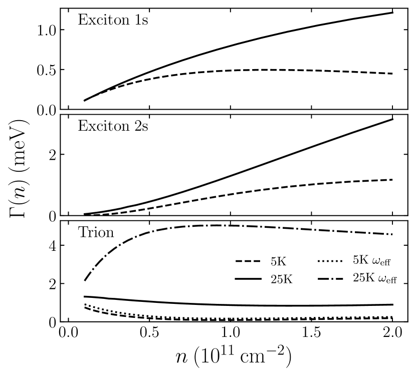
Figure 1: Line width broadening of monolayer MoSe₂ as a function of electron doping density for BN-encapsulated ($\varepsilon_{0}=4.5$)Gielisse et al. (1967) monolayers. The following parameters were used: in the exciton calculation, the effective Bohr radii $\lambda_{0}=10.3$ and in the case of the trion, $\lambda_{1}=\lambda_{0}$ and $\lambda_{2}=25.2$ Å.Berkelbach et al. (2013) In the exciton 2s elastic scattering, $a=7.79$ Å and $b=6.20$ Å (see Appendix B.4). The electron (hole) effective masses employed were $0.49$ $(0.61)$ (in units of $m_{0}$),Rasmussen and Thygesen (2015) and the polarizability $\chi_{\mathrm{2D}}=8.23$ Å.Berkelbach et al. (2013) In the case of exciton elastic scattering, the singlet and triplet contributions are identical as the exchange contribution to the potential dominates; trion triplet states are not considered. Additionally, screening using the effective frequency-dependent dielectric function (see Eq. 16) are presented for the trion, as the effective screening does not appear to affect the exciton line width.

We first discuss trion line broadening. For doping levels $n>0.4\times 10^{11}$ cm${}^{-2},$ the trion line width in all cases is largely independent of doping density. The upturn seen in the static screening trion line width as doping density decreases is likely an artifact of behavior embedded in the function $\varepsilon_{2}(q).$ Indeed, a suppression of the $q^{-3}$ behavior for large $q$ of this function leads to an essentially flat trion line width as a function of doping level, similar to that seen in Fermi-polaron-like theories and in some experiments.Astakhov et al. (2000); Smoleński et al. (2018) It should be noted that in these approaches, however, the trion line broadening is controlled by a phenomenological input parameter.Efimkin and MacDonald (2017) Here, our fully microscopic approach allows for the microscopic extraction of the magnitude and temperature dependence of the trion line width. While the static and effective frequency-dependent screening cases are largely in agreement at low $T,$ the same cannot be said for results at 25K. Given the subtle changes in the scattering matrix elements except at small $q,$ this difference likely arises from the larger accessible density of states available at higher densities away from $\omega=0$ in the screening function.

We now turn to the broadening of the exciton line. Unlike the trion case, the exciton line width monotonically increases as a function of doping density at low values of $n$ in the 25 K case. This is again in agreement with experimental expectations as well as the behavior found in many-body approaches.Efimkin and MacDonald (2017); Sidler et al. (2017b); Chang et al. (2018) In particular, in these latter theoretical approaches, an approximately linear dependence of the line width on doping manifests over a much wider doping density range for the exciton line. The very same behavior arises from the Golden Rule at extremely low doping. The decrease of the slope of the line width as $n$ increases, most clearly demonstrated in the near-plateau of the 5 K exciton line widths above $n=0.8\times 10^{11}$ cm${}^{-2},$ is a signature of the breakdown of the Golden Rule. Specifically, due to the $\varepsilon_{\mathrm{F}}/k_{\mathrm{B}}T$ term in the Fermi-Dirac distribution function, the crossover from the non-degenerate to the degenerate electron gas limit will induce a change in the doping dependence of the excitonic line width from a linear scaling $\Gamma\sim n$ at low doping to an eventual plateau $\sim k_{\mathrm{B}}T,$ and then an unphysical decline with increasing $n.$ This same trend is reported in Ref. Ramon et al., 2003 for the quantum well case. We systematically examine this behavior in Fig. 2, which shows the doping and temperature dependence of this behavior. If one focuses on the more physically-described regime $n<0.8\times 10^{11}$ cm${}^{-2},$ it is observed that, unlike in the trion case, doping-induced exciton line broadening is largely insensitive to temperature variations in the range $T=5$-$25$ K. Furthermore, given the fact that phonon-induced line broadening is suppressed at these temperatures, doping induced line broadening effects may be observable at $T=5$ K in clean, encapsulated samples even for doping densities as low as $n\sim 2\times 10^{11}$ cm${}^{-2},$ especially with respect to the 2s line, where the line broadening effects appear to be slightly enhanced compared to the ground state.

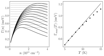
Figure 2: Doping dependence of the 1s exciton line width at temperatures $T=5,6,...,15$ K (left). Parameters describe monolayer MoSe₂, as seen in Fig 1. Lower line widths correspond to lower temperatures. The horizontal dashed lines show the plateau location. The value of the maximum (plateau) is also plotted as a function of temperature, showing clear linear behavior at low $T$ (right).

IV Conclusion

In this work we have employed perturbation theory to calculate the rates of electron-exciton and electron-trion scattering in monolayer TMDCs in the low doping density limit. Our approach is fully microscopic with respect to all input parameters and functions, including matrix elements and the dielectric screening model. On the other hand, it is expected that the Fermi Golden Rule should break down at low doping densities close to the degeneracy crossover of the electron gas in the monolayer, and some caution must be exercised with respect to the use the forms of the dielectric screening functions employed here.Glazov and Chernikov (2018) Avoiding these approximations allows for the description of a much broader range of doping, but requires a full frequency-dependent many-body treatment.Efimkin and MacDonald (2017); Sidler et al. (2017b); Chang and Reichman (2019)

Accepting the above limitations, the calculations presented here still allow for some important conclusions to be drawn. First, we find that with a reasonable treatment dielectric environment, exciton line widths arising from exciton-electron scattering on the order of 1 meV or higher are possible at low temperatures in the low doping regime accessible in encapsulated, graphene-gated samples. Thus, even mild doping may provide a line broadening mechanism that can compete with (but not necessarily exceed) lifetime and phonon-related broadening in this regime. As expected from previous many-body calculations in the very low doping regime, the growth of the excitonic line width is monotonic with increasing $n$, while the trion line width is largely insensitive to doping. However we find that the trion line width is sensitive to temperature variations even over the small range $T=5$-$25$ K, a somewhat unexpected feature from the standpoint of many-body theories such as that of Ref.Efimkin and MacDonald (2017) where the trion line width is partly described by a phenomenological input parameter. Lastly, we find that excited state exction line broadening is somewhat larger and shows more sensitivity to increases in doping levels. Future work should be devoted to testing the veracity of these predictions and to understand how they merge with many-body approaches which have been applied to study the higher doping density regime.Fey et al. (2019)

In conclusion, we have provided a microscopic model for understanding how the scattering of excitons and trions surrounded by an electron gas in monolayer TMDCs may induce line broadening in the very low doping density limit at low temperatures. A more detailed effort aimed at placing these contributions in the context of other mechanisms, such as exciton-phonon scattering, is worth of future study. In addition, the approach adopted here may be of use for the calculation of the rates of processes such as Auger recombinationHuang and Krauss (2006); Wang et al. (2006); Hu et al. (2016) in dimensionally-confined systems. These and related topics will the subject of future investigations.

Appendix A RPA Polarizability

Following the definition in Stern,Stern (1967) in this appendix we present the frequency-dependent 2D electron gas polarizability, $\chi,$ and its $\omega\rightarrow 0$ limit. The general form of $\chi$ is $\chi(q,\omega)=\chi_{1}(q,\omega)+i\chi_{2}(q,\omega),$ where

$$\chi_{1}(z,\tilde{u})=\frac{e^{2}m}{\hbar^{2}q^{2}\pi}\left\{1-\frac{C_{-}(z,\tilde{u})}{2}\sqrt{\left(1-\tilde{u}\right)^{2}-z^{-2}}-\frac{C_{+}(z,\tilde{u})}{2}\sqrt{\left(1+\tilde{u}\right)^{2}-z^{-2}}\right\}$$ (17)

and

$$\chi_{2}(z,\tilde{u})=\frac{e^{2}m}{\hbar^{2}q^{2}\pi}\left\{\frac{D_{-}(z,\tilde{u})}{2}\sqrt{z^{-2}-\left(1-\tilde{u}\right)^{2}}-\frac{D_{+}(z,\tilde{u})}{2}\sqrt{z^{-2}-\left(1+\tilde{u}\right)^{2}}\right\},$$ (18)

where $z\equiv q/2k_{\mathrm{F}}$ and $\tilde{u}\equiv 2\omega m/\hbar q^{2}.$ Note that the quantities in the braces, $\{\cdot\},$ are dimensionless. The functions $C$ and $D$ are defined as follows,

$$C_{\pm}(z,\tilde{u})\equiv\begin{cases}(z\pm\tilde{u})/|z\pm\tilde{u}|&\text{if }|z\pm\tilde{u}|>1\\ 0&\text{otherwise}\end{cases}$$ (19)

and

$$D_{\pm}(z,\tilde{u})\equiv\begin{cases}0&\text{if }|z\pm\tilde{u}|>1\\ 1&\text{otherwise}\end{cases}.$$ (20)

In the static approximation we note that $\chi_{2}(q,0)=0$ and $\chi_{1}$ reduces to (15), where generally

$$\varepsilon_{2}(q,\omega)=2\pi B(q,\omega)\chi(q/2k_{\mathrm{F}},2\omega m/\hbar q^{2}),$$ (21)

and $B(q,\omega)=\sqrt{q^{2}-\varepsilon_{0}\omega^{2}c^{-2}}.$

Appendix B Exciton-electron elastic scattering

In this appendix, we outline the details of the $X+e^{-}\rightarrow X+e^{-}$ scattering calculation, including accounting for electron spin. Here, and in Appendix C, we follow closely with the approach of Ref. Ramon et al., 2003, generalizing to the strict 2D limit and filling in necessary details.

In the following, it will be useful to keep in mind the electron and hole anti-commutation relations

$$\{d_{\mathbf{k}}^{s\dagger},c_{\mathbf{k}^{\prime}}^{s^{\prime}\dagger}\}=\{d_{\mathbf{k}}^{s\dagger},c_{\mathbf{k}^{\prime}}^{s^{\prime}}\}=\{d_{\mathbf{k}}^{s},c_{\mathbf{k}^{\prime}}^{s^{\prime}\dagger}\}=\{d_{\mathbf{k}}^{s},c_{\mathbf{k}^{\prime}}^{s^{\prime}}\}=0,$$

(electrons and holes always anti-commute) and,

$$\{x_{\mathbf{k}}^{s},x_{\mathbf{k}^{\prime}}^{s^{\prime}}\}=\{x_{\mathbf{k}}^{s\dagger},x_{\mathbf{k}^{\prime}}^{s^{\prime}\dagger}\}=0;\quad\{x_{\mathbf{k}}^{s},x_{\mathbf{k}^{\prime}}^{s^{\prime}\dagger}\}=\delta_{\mathbf{k}\mathbf{k}^{\prime}}\delta_{ss^{\prime}},$$

where $x=c,d.$ Also, recall that $\psi_{\mathbf{k}_{\mathrm{e}}}$ ends up as a global phase factor in the expression for the scattering rate, and will be ignored in the following derivations.

B.1 General form of the matrix elements

A prudent first step to computing (5) is to split up $V$ into its constituent parts and evaluate them independently on the initial state $\ket{\mathbf{k}_{\mathrm{x}}^{\alpha},\mathbf{k}_{\mathrm{e}}^{\beta}},$ where spin indexes have been added as superscripts (the exciton spin references the electron; hole spin will not be important). In the case of the electron-hole component, we have

$$\begin{split}V_{\mathrm{e}\mathrm{h}}\ket{\mathbf{k}_{\mathrm{x}}^{\alpha},\mathbf{k}_{\mathrm{e}}^{\beta}}&=\sum_{\mathbf{k}^{\prime}\mathbf{q}^{\prime}}v_{q^{\prime}}\phi^{*}\underbrace{c_{-\mathbf{k}^{\prime}+\mathbf{q}^{\prime}}^{\alpha\dagger}d_{\mathbf{k}_{\mathrm{x}}+\mathbf{k}^{\prime}-\mathbf{q}^{\prime}}^{\dagger}}_{\text{self-interaction}}c_{\mathbf{k}_{\mathrm{e}}}^{\beta\dagger}\ket{0}\\ &-\sum_{\mathbf{k}^{\prime}\mathbf{q}^{\prime}}v_{q^{\prime}}\phi^{*}c_{-\mathbf{k}^{\prime}}^{\alpha\dagger}d_{\mathbf{k}_{\mathrm{x}}+\mathbf{k}^{\prime}-\mathbf{q}^{\prime}}^{\dagger}c_{\mathbf{k}_{\mathrm{e}}+\mathbf{q}^{\prime}}^{\beta\dagger}\ket{0},\end{split}$$ (22)

where $\phi^{*}\equiv\phi^{*}_{\alpha_{\mathrm{x}}\mathbf{k}_{\mathrm{x}}+\mathbf{k}^{\prime}}.$ The first term in the above equation only contains information about the exciton interacting with itself (self-interaction) and is therefore discarded. The electron-electron component is calculated in a similar fashion and does not contain self-interaction terms:

$$V_{\mathrm{e}\mathrm{e}}\ket{\mathbf{k}_{\mathrm{x}}^{\alpha},\mathbf{k}_{\mathrm{e}}^{\beta}}=\sum_{\mathbf{k}^{\prime}\mathbf{q}^{\prime}}v_{q^{\prime}}\phi^{*}c_{-\mathbf{k}^{\prime}-\mathbf{q}^{\prime}}^{\alpha\dagger}d_{\mathbf{k}_{\mathrm{x}}+\mathbf{k}^{\prime}}^{\dagger}c_{\mathbf{k}_{\mathrm{e}}+\mathbf{q}^{\prime}}^{\beta\dagger}\ket{0}.$$ (23)

From here by direct computation we find the general matrix elements of the electron-exciton elastic scattering process to be

$$\matrixelement{(\mathbf{k}_{\mathrm{x}}+\mathbf{q})^{\theta},(\mathbf{k}_{\mathrm{e}}-\mathbf{q})^{\omega}}{V_{\mathrm{e}\mathrm{h}}}{\mathbf{k}_{\mathrm{x}}^{\alpha},\mathbf{k}_{\mathrm{e}}^{\beta}}=\\ -\sum_{\mathbf{k}^{\prime\prime}\mathbf{k}^{\prime}\mathbf{q}^{\prime}}\phi_{1}\phi_{2}^{*}v_{q^{\prime}}(\delta_{\mathbf{k}^{\prime\prime},\mathbf{k}^{\prime}}^{\theta\alpha}\delta_{-\mathbf{q},\mathbf{q}^{\prime}}^{\omega\beta}-\delta_{-\mathbf{k}^{\prime\prime},\mathbf{k}_{\mathrm{e}}+\mathbf{q}^{\prime}}^{\theta\beta}\delta_{\mathbf{k}^{\prime},\mathbf{k}_{\mathrm{e}}-\mathbf{q}}^{\omega\alpha}),$$ (24)

where $\phi_{1}\phi_{2}^{*}\equiv\phi_{\alpha_{\mathrm{x}}\mathbf{k}_{\mathrm{x}}+\alpha_{\mathrm{x}}\mathbf{q}+\mathbf{k}^{\prime\prime}}\phi_{\alpha_{\mathrm{x}}\mathbf{k}_{\mathrm{x}}+\mathbf{k}^{\prime}}^{*}.$ Explicitly, this is

$$\matrixelement{(\mathbf{k}_{\mathrm{x}}+\mathbf{q})^{\theta},(\mathbf{k}_{\mathrm{e}}-\mathbf{q})^{\omega}}{V_{\mathrm{e}\mathrm{h}}}{\mathbf{k}_{x}^{\alpha},\mathbf{k}_{e}^{\beta}}=\\ v_{q}\delta_{\theta\alpha}\delta_{\omega\beta}\sum_{\mathbf{k}^{\prime}}\phi_{\alpha_{\mathrm{x}}\mathbf{k}_{\mathrm{x}}+\alpha_{\mathrm{x}}\mathbf{q}+\mathbf{k}^{\prime}}\phi_{\alpha_{\mathrm{x}}\mathbf{k}_{\mathrm{x}}+\mathbf{k}^{\prime}}\\ -\phi_{\alpha_{\mathrm{x}}\mathbf{k}_{\mathrm{x}}-\mathbf{k}_{\mathrm{e}}+\mathbf{q}}\delta_{\theta\beta}\delta_{\omega\alpha}\sum_{\mathbf{k}^{\prime}}\phi_{\alpha_{\mathrm{x}}\mathbf{k}_{\mathrm{x}}+\alpha_{\mathrm{x}}\mathbf{q}-\mathbf{k}_{\mathrm{e}}-\mathbf{k}^{\prime}}v_{k^{\prime}},$$ (25)

which can be separated into direct (corresponding to $v_{q}$) and exchange ($v_{k^{\prime}}$) contributions. It is also observed that for practical computation $\phi=\phi^{*}$ and thus the complex conjugation is dropped. The electron-electron term is computed

$$\matrixelement{(\mathbf{k}_{\mathrm{x}}+\mathbf{q})^{\theta},(\mathbf{k}_{\mathrm{e}}-\mathbf{q})^{\omega}}{V_{\mathrm{e}\mathrm{e}}}{\mathbf{k}_{\mathrm{x}}^{\alpha},\mathbf{k}_{\mathrm{e}}^{\beta}}=\\ \sum_{\mathbf{k}^{\prime\prime}\mathbf{k}^{\prime}\mathbf{q}^{\prime}}\phi_{1}\phi_{2}^{*}v_{q^{\prime}}(\delta_{\mathbf{k}^{\prime\prime},\mathbf{k}^{\prime}+\mathbf{q}^{\prime}}^{\theta\alpha}\delta_{\mathbf{q},-\mathbf{q}^{\prime}}^{\omega\beta}\\ -\delta_{-\mathbf{k}^{\prime\prime},\mathbf{k}_{\mathrm{e}}+\mathbf{q}^{\prime}}^{\theta\beta}\delta_{-\mathbf{k}^{\prime}-\mathbf{q}^{\prime},\mathbf{k}_{\mathrm{e}}-\mathbf{q}}^{\omega\alpha})$$ (26)

and simplified in a similar fashion,

$$\matrixelement{(\mathbf{k}_{\mathrm{x}}+\mathbf{q})^{\theta},(\mathbf{k}_{\mathrm{e}}-\mathbf{q})^{\omega}}{V_{\mathrm{e}\mathrm{e}}}{\mathbf{k}_{\mathrm{x}}^{\alpha},\mathbf{k}_{\mathrm{e}}^{\beta}}=\\ v_{q}\delta_{\theta\alpha}\delta_{\omega\beta}\sum_{\mathbf{k}^{\prime}}\phi_{\alpha_{\mathrm{x}}\mathbf{k}_{\mathrm{x}}-\beta_{\mathrm{x}}\mathbf{q}+\mathbf{k}^{\prime}}\phi_{\alpha_{\mathrm{x}}\mathbf{k}_{\mathrm{x}}+\mathbf{k}^{\prime}}\\ -\delta_{\theta\beta}\delta_{\omega\alpha}\sum_{\mathbf{k}^{\prime}}\phi_{\alpha_{\mathrm{x}}\mathbf{k}_{\mathrm{x}}+\alpha_{\mathrm{x}}\mathbf{q}-\mathbf{k}_{\mathrm{e}}-\mathbf{k}^{\prime}}\phi_{\alpha_{\mathrm{x}}\mathbf{k}_{\mathrm{x}}+\mathbf{q}-\mathbf{k}_{\mathrm{e}}-\mathbf{k}^{\prime}}v_{k^{\prime}}.$$ (27)

Combining terms into direct and exchange contributions, we have

$$V^{\mathrm{D}}(\mathbf{q},\mathbf{k}_{\mathrm{e}},\mathbf{k}_{\mathrm{x}})=v_{q}\delta_{\theta\alpha}\delta_{\omega\beta}\sum_{\mathbf{k}^{\prime}}\phi_{\alpha_{\mathrm{x}}\mathbf{k}_{\mathrm{x}}+\mathbf{k}^{\prime}}\\ \times[\phi_{\alpha_{\mathrm{x}}\mathbf{k}_{\mathrm{x}}-\beta_{\mathrm{x}}\mathbf{q}+\mathbf{k}^{\prime}}-\phi_{\alpha_{\mathrm{x}}\mathbf{k}_{\mathrm{x}}+\alpha_{\mathrm{x}}\mathbf{q}+\mathbf{k}^{\prime}}],$$ (28)

where the Kronecker delta functions ensure the proper spins are paired, and

$$V^{\mathrm{XC}}(\mathbf{q},\mathbf{k}_{\mathrm{e}},\mathbf{k}_{\mathrm{x}})=-\delta_{\theta\beta}\delta_{\omega\alpha}\sum_{\mathbf{k}^{\prime}}v_{k^{\prime}}\phi_{\alpha_{x}\mathbf{q}-\Delta\mathbf{k}_{\mathrm{x}}+\mathbf{k}^{\prime}}\\ \times[\phi_{\mathbf{q}-\Delta\mathbf{k}_{\mathrm{x}}+\mathbf{k}^{\prime}}-\phi_{\mathbf{q}-\Delta\mathbf{k}_{\mathrm{x}}}],$$ (29)

where $\Delta\mathbf{k}_{\mathrm{x}}\equiv\mathbf{k}_{\mathrm{e}}-\alpha_{\mathrm{x}}\mathbf{k}_{\mathrm{x}}.$

B.2 Spin contributions

Both the $V_{\mathrm{e}\mathrm{e}}$ and $V_{\mathrm{e}\mathrm{h}}$ terms can be split into clear direct and exchange contributions such that in the individual electron spin basis,

$$\matrixelement{\theta\omega}{V}{\alpha\beta}=\delta_{\theta\alpha}\delta_{\omega\beta}V^{\mathrm{D}}+\delta_{\theta\beta}\delta_{\omega\alpha}V^{\mathrm{XC}}.$$

If the incident and exciton electrons are in a singlet configuration, we have to consider all contributions from the singlet state $\ket{S}=(\ket{\uparrow\downarrow}-\ket{\downarrow\uparrow})/\sqrt{2},$

$$\matrixelement{S}{V}{S}=\frac{1}{2}(\matrixelement{\uparrow\downarrow}{V}{\uparrow\downarrow}+\text{cc.}-\matrixelement{\uparrow\downarrow}{V}{\downarrow\uparrow}-\text{cc.}),$$

which in the specified basis is

$$V_{S}\equiv\matrixelement{S}{V}{S}=V^{\mathrm{D}}-V^{\mathrm{XC}}.$$

By inspection, any of the triplet configurations are

$$V_{T}\equiv\matrixelement{T}{V}{T}=V^{\mathrm{D}}+V^{\mathrm{XC}}.$$

In the case of the exciton case, the singlet and triplet contributions are essentially identical, since the exchange contribution dominates, meaning $\absolutevalue{V_{S}}^{2}\approx\absolutevalue{V_{T}}^{2};$ for the trion, we do not consider triplet states.

B.3 1s$\rightarrow$1s scattering

With the assumption that the exciton wave function $\phi$ is in the parameterized ground state (1s) given by (3), the direct interaction has an analytic form. Noting that

$$\sum_{\mathbf{k}}\rightarrow\frac{A}{(2\pi)^{2}}\int\differential^{2}k,\quad\mathbf{k}\in\mathbb{R}^{2},$$

and that the convolution

$$\int\differential^{2}k^{\prime}g(\lambda k^{\prime})g(\lambda^{\prime}|\mathbf{q}\pm\mathbf{k}^{\prime}|)=\frac{2\pi}{(\lambda+\lambda^{\prime})^{2}}g\left(\frac{\lambda\lambda^{\prime}q}{\lambda+\lambda^{\prime}}\right),$$ (30)

the direct terms simplify to (dropping the spin Kronecker deltas)

$$V^{\mathrm{D}}_{\mathrm{1s}}(q)=\frac{2\pi e^{2}}{Aq\varepsilon(q)}\left[g(\lambda\beta_{\mathrm{x}}q/2)-g(\lambda\alpha_{\mathrm{x}}q/2)\right].$$ (31)

The exchange terms do not simplify and must be evaluated numerically,

$$V^{\mathrm{XC}}_{1s}(\mathbf{q},\mathbf{k}_{\mathrm{e}},\mathbf{k}_{\mathrm{x}})=-\frac{4e^{2}\lambda^{2}}{A}\int\frac{\differential^{2}k^{\prime}}{k^{\prime}\varepsilon(k^{\prime})}\\ \times g(\lambda|\alpha_{\mathrm{x}}\mathbf{q}-\Delta\mathbf{k}_{\mathrm{x}}+\mathbf{k}^{\prime}|)\\ \times\left[g(\lambda|\mathbf{k}_{1}+\mathbf{q}-\Delta\mathbf{k}_{\mathrm{x}}|)-g(\lambda|\mathbf{q}-\Delta\mathbf{k}_{\mathrm{x}}|)\right].$$ (32)

These results have been previously derived for scattering in finite quantum wellsRamon et al. (2003) and match the results above in the 2D analytic limit. Here, $\lambda=\lambda_{0}=10.3$ Å is the exciton effective Bohr radius, and $\alpha_{\mathrm{x}}=m_{\mathrm{e}}/M_{\mathrm{x}}$ is the mass ratio of the exciton, $\beta_{\mathrm{x}}=1-\alpha_{\mathrm{x}},$ $m_{\mathrm{e}}=0.49m_{0}$ and $M_{\mathrm{x}}=m_{\mathrm{e}}+m_{\mathrm{h}},$ where $m_{\mathrm{h}}=0.61m_{0}.$

B.4 2s$\rightarrow$2s scattering

To compute the excited state (2s) exciton elastic scattering line width, we parameterize a radial 2s hydrogen wave function

$$\phi^{\mathrm{2s}}(r,a,b)\propto\left(2-\frac{r}{b}\right)e^{-r/2a}$$ (33)

in terms of an effective Bohr radius $a$ and a secondary parameter $b$ chosen to ensure orthogonality to the 1s state. An initial fit to the first excited state exact-diagonalization result of the Wannier exciton in a 2D Keldysh potential yielded length scales $a=7.79$ Å and $b=5.33$ Å, the latter of which was modified to $b=6.20$ Å to ensure orthogonality. Fourier transforming to momentum-space yields

$$\phi_{k}^{\mathrm{2s}}=N_{\mathrm{2s}}\left[\frac{16\pi a^{2}}{(1+4a^{2}k^{2})^{3/2}}-\frac{2\pi\left(\frac{1}{2a^{2}}-k^{2}\right)}{b\left(\frac{1}{4a^{2}}+k^{2}\right)^{5/2}}\right]$$ (34)

with normalization

$$N_{\mathrm{2s}}=\sqrt{\frac{b^{2}}{4\pi a^{2}A(3a^{2}-4ab+2b^{2})}}.$$

Matrix elements are computed by making the substitution $\phi\rightarrow\phi^{\mathrm{2s}}$ in (28) and (29) numerically performing the 2D integrals.

Appendix C Trion-electron elastic scattering

The details of the $T+e^{-}\rightarrow T+e^{-}$ scattering process are significantly more involved than the exciton case. The introduction of an extra electron manifests as another pair of creation and annihilation operators in the matrix element evaluation and adds many more terms. While the calculation is longer, it is no more conceptually difficult. In this appendix, we present the detailed derivation of the matrix elements for a two dimensional system, which coincide with the results for the 3D quantum well in the $L\rightarrow 0$ limit.Ramon et al. (2003)

The total elastic scattering matrix element $\mathcal{V}(\mathbf{q},\mathbf{k}_{\mathrm{e}},\mathbf{k}_{\mathrm{t}})$ is calculated by first computing the action of $V|\mathbf{k}_{\mathrm{t}},\mathbf{k}_{\mathrm{e}}\rangle.$ This not only simplifies the number of operator contractions, it also allows for removal of self-interaction terms (those characterized by internal interactions between electrons and holes within the trion), as they do not contribute to the scattering matrix elements (similar to that of the exciton scattering case). To begin, we first evaluate the general contraction, which is used during the evaluation of (12),

$$c_{1}c_{2}^{\dagger}c_{3}^{\dagger}c_{4}^{\dagger}\ket{0}=[\delta_{12}c_{3}^{\dagger}c_{4}^{\dagger}-\delta_{13}c_{2}^{\dagger}c_{4}^{\dagger}+\delta_{14}c_{2}^{\dagger}c_{3}^{\dagger}]\ket{0},$$ (35)

where in (36), $1\equiv(\mathbf{k}_{1}^{\prime},z_{1}^{\prime},s^{\prime}),$ $2\equiv(-\mathbf{k}_{1},z_{1},s_{1}),$ $3\equiv(-\mathbf{k}_{2},z_{2},s_{2}),$ and $4\equiv(\mathbf{k}_{\mathrm{e}},z_{\mathrm{e}},s_{\mathrm{e}}),$ as this will be useful in computing both $V_{\mathrm{e}\mathrm{h}}|\mathbf{k}_{\mathrm{t}},\mathbf{k}_{\mathrm{e}}\rangle$ and $V_{\mathrm{e}\mathrm{e}}|\mathbf{k}_{\mathrm{t}},\mathbf{k}_{\mathrm{e}}\rangle.$ In following calculations, hole operators will be ignored, as they do not contribute additional constraints or prefactors to the line width calculations. Moreover, $V_{\mathrm{e}\mathrm{h}}|\mathbf{k}_{\mathrm{t}},\mathbf{k}_{\mathrm{e}}\rangle$ evaluates to

$$\begin{split}V_{\mathrm{e}\mathrm{h}}\ket{\mathbf{k}_{\mathrm{t}},\mathbf{k}_{\mathrm{e}}}&=-\sum_{\begin{subarray}{c}\mathbf{k}_{1},\mathbf{k}_{2},\mathbf{k}_{1}^{\prime},\mathbf{q}^{\prime}\\ s_{1},s_{2},s_{\mathrm{e}},s^{\prime}\end{subarray}}v_{q^{\prime}}\xi_{S}^{*}(s_{1},s_{2})\Phi_{\alpha_{\mathrm{t}}\mathbf{k}_{\mathrm{t}}+\mathbf{k}_{1},\alpha_{t}\mathbf{k}_{\mathrm{t}}+\mathbf{k}_{2}}^{*}\psi_{\mathbf{k}_{\mathrm{e}}}^{*}c_{\mathbf{k}_{1}^{\prime}+\mathbf{q}^{\prime}}^{s^{\prime}\dagger}c_{\mathbf{k}_{1}^{\prime}}^{s^{\prime}}c_{-\mathbf{k}_{1}}^{s_{1}\dagger}c_{-\mathbf{k}_{2}}^{s_{2}\dagger}c_{\mathbf{k}_{e}}^{s_{e}\dagger}\ket{0}\\ &=-\sum_{\begin{subarray}{c}\mathbf{k}_{1},\mathbf{k}_{2},\mathbf{q}^{\prime}\\ s_{1},s_{2},s_{e}\end{subarray}}\xi_{S}^{*}(s_{1},s_{2})\Phi_{\alpha_{\mathrm{t}}\mathbf{k}_{\mathrm{t}}+\mathbf{k}_{1},\alpha_{\mathrm{t}}\mathbf{k}_{\mathrm{t}}+\mathbf{k}_{2}}^{*}\psi_{\mathbf{k}_{\mathrm{e}}}^{*}v_{q^{\prime}}\left\{c_{-\mathbf{k}_{1}+\mathbf{q}^{\prime}}^{s_{1}\dagger}c_{-\mathbf{k}_{2}}^{s_{2}\dagger}c_{\mathbf{k}_{\mathrm{e}}}^{s_{\mathrm{e}}\dagger}-c_{-\mathbf{k}_{2}+\mathbf{q}^{\prime}}^{s_{2}\dagger}c_{-\mathbf{k}_{1}}^{s_{1}\dagger}c_{\mathbf{k}_{\mathrm{e}}}^{s_{\mathrm{e}}\dagger}+c_{\mathbf{k}_{e}+\mathbf{q}^{\prime}}^{s_{\mathrm{e}}\dagger}c_{-\mathbf{k}_{1}}^{s_{1}\dagger}c_{-\mathbf{k}_{2}}^{s_{2}\dagger}\right\}\ket{0}.\end{split}$$ (36)

The first two terms correspond to self-interactions between the internal electrons and holes of the trion. This is most easily seen by observing that after the action of $V_{\mathrm{e}\mathrm{h}}$ on the trion-free electron state, the initial incident electron momentum $\mathbf{k}_{\mathrm{e}}$ remains unchanged in the final creation operator. In the last term, however, we see that a momentum exchange of $\mathbf{q}^{\prime}$ has taken place.

The electron-electron terms corresponding to $V_{\mathrm{e}\mathrm{e}}\ket{\mathbf{k}_{\mathrm{t}},\mathbf{k}_{\mathrm{e}}}$ are calculated similarly. As in the electron-hole case, we begin by performing the right-most contraction

$$\begin{split}c_{1}c_{2}c_{3}^{\dagger}c_{4}^{\dagger}c_{5}^{\dagger}\ket{0}&=[\delta_{15}\delta_{24}-\delta_{14}\delta_{25}]c_{3}^{\dagger}\ket{0}\\ &+[\delta_{13}\delta_{25}-\delta_{15}\delta_{23}]c_{4}^{\dagger}\ket{0}\\ &+[\delta_{14}\delta_{23}-\delta_{13}\delta_{24}]c_{5}^{\dagger}\ket{0},\end{split}$$ (37)

where in (37) and (38) $1\equiv(\mathbf{k}_{2}^{\prime},s_{2}^{\prime}),$ $2\equiv(\mathbf{k}_{1}^{\prime},s_{1}^{\prime}),$ $3\equiv(-\mathbf{k}_{1},s_{1}),$ $4\equiv(-\mathbf{k}_{2},s_{2}),$ $5\equiv(\mathbf{k}_{\mathrm{e}},s_{\mathrm{e}}).$ In similar fashion, $V_{\mathrm{e}\mathrm{e}}\ket{\mathbf{k}_{\mathrm{t}},\mathbf{k}_{\mathrm{e}}}$ is thus found to be

$$\begin{split}V_{\mathrm{e}\mathrm{e}}|\mathbf{k}_{\mathrm{t}},\mathbf{k}_{\mathrm{e}}\rangle&=\frac{1}{2}\sum_{\begin{subarray}{c}\mathbf{k}_{1},\mathbf{k}_{2},\mathbf{k}_{1}^{\prime},\mathbf{k}_{2}^{\prime},\mathbf{q}^{\prime}\\ s_{1},s_{2},s_{\mathrm{e}},s_{1}^{\prime},s_{2}^{\prime}\end{subarray}}\xi_{S}^{*}(s_{1},s_{2})\Phi_{\alpha_{\mathrm{t}}\mathbf{k}_{\mathrm{t}}+\mathbf{k}_{1},\alpha_{\mathrm{t}}\mathbf{k}_{\mathrm{t}}+\mathbf{k}_{2}}^{*}\psi_{\mathbf{k}_{\mathrm{e}}}^{*}v_{q^{\prime}}c_{\mathbf{k}_{1}^{\prime}+\mathbf{q}^{\prime}}^{s_{1}^{\prime}\dagger}c_{\mathbf{k}_{2}^{\prime}-\mathbf{q}^{\prime}}^{s_{2}^{\prime}\dagger}c_{\mathbf{k}_{2}^{\prime}}^{s_{2}^{\prime}}c_{\mathbf{k}_{1}^{\prime}}^{s_{1}^{\prime}}c_{-\mathbf{k}_{1}}^{s_{1}\dagger}c_{-\mathbf{k}_{2}}^{s_{2}\dagger}c_{\mathbf{k}_{\mathrm{e}}}^{s_{\mathrm{e}}\dagger}\ket{0}\\ &=\frac{1}{2}\sum_{\begin{subarray}{c}\mathbf{k}_{1},\mathbf{k}_{2},\mathbf{q}^{\prime}\\ s_{1},s_{2},s_{\mathrm{e}}\end{subarray}}\xi_{S}^{*}(s_{1},s_{2})\Phi_{\alpha_{\mathrm{t}}\mathbf{k}_{\mathrm{t}}+\mathbf{k}_{1},\alpha_{\mathrm{t}}\mathbf{k}_{\mathrm{t}}+\mathbf{k}_{2}}^{*}\psi_{\mathbf{k}_{\mathrm{e}}}^{*}v_{q^{\prime}}\big{\{}c_{-\mathbf{k}_{2}+\mathbf{q}^{\prime}}^{s_{2}\dagger}c_{\mathbf{k}_{\mathrm{e}}-\mathbf{q}^{\prime}}^{s_{\mathrm{e}}\dagger}c_{-\mathbf{k}_{1}}^{s_{1}\dagger}-c_{\mathbf{k}_{\mathrm{e}}+\mathbf{q}^{\prime}}^{s_{\mathrm{e}}\dagger}c_{-\mathbf{k}_{2}-\mathbf{q}^{\prime}}^{s_{2}\dagger}c_{-\mathbf{k}_{1}}^{s_{1}\dagger}\\ &+c_{\mathbf{k}_{\mathrm{e}}+\mathbf{q}^{\prime}}^{s_{\mathrm{e}}\dagger}c_{-\mathbf{k}_{1}-\mathbf{q}^{\prime}}^{s_{1}\dagger}c_{-\mathbf{k}_{2}}^{s_{2}\dagger}-c_{-\mathbf{k}_{1}+\mathbf{q}^{\prime}}^{s_{1}\dagger}c_{\mathbf{k}_{\mathrm{e}}-\mathbf{q}^{\prime}}^{s_{\mathrm{e}}\dagger}c_{-\mathbf{k}_{2}}^{s_{2}\dagger}+c_{-\mathbf{k}_{1}+\mathbf{q}^{\prime}}^{s_{1}\dagger}c_{-\mathbf{k}_{2}-\mathbf{q}^{\prime}}^{s_{2}\dagger}c_{\mathbf{k}_{\mathrm{e}}}^{s_{\mathrm{e}}\dagger}-c_{-\mathbf{k}_{2}+\mathbf{q}^{\prime}}^{s_{2}\dagger}c_{-\mathbf{k}_{1}-\mathbf{q}^{\prime}}^{s_{1}\dagger}c_{\mathbf{k}_{\mathrm{e}}}^{s_{\mathrm{e}}\dagger}\big{\}}\ket{0}\\ &=\sum_{\begin{subarray}{c}\mathbf{k}_{1},\mathbf{k}_{2},\mathbf{q}^{\prime}\\ s_{1},s_{2},s_{e}\end{subarray}}\xi_{S}^{*}(s_{1},s_{2})\Phi_{\alpha_{\mathrm{t}}\mathbf{k}_{\mathrm{t}}+\mathbf{k}_{1},\alpha_{\mathrm{t}}\mathbf{k}_{\mathrm{t}}+\mathbf{k}_{2}}^{*}\psi_{\mathbf{k}_{\mathrm{e}}}^{*}v_{q^{\prime}}\\ &\times\big{\{}c_{-\mathbf{k}_{1}}^{s_{1}\dagger}c_{-\mathbf{k}_{2}-\mathbf{q}^{\prime}}^{s_{2}\dagger}c_{\mathbf{k}_{\mathrm{e}}+\mathbf{q}^{\prime}}^{s_{\mathrm{e}}\dagger}+c_{-\mathbf{k}_{1}-\mathbf{q}^{\prime}}^{s_{1}\dagger}c_{-\mathbf{k}_{2}}^{s_{2}\dagger}c_{\mathbf{k}_{\mathrm{e}}+\mathbf{q}^{\prime}}^{s_{\mathrm{e}}\dagger}+c_{-\mathbf{k}_{1}-\mathbf{q}^{\prime}}^{s_{1}\dagger}c_{-\mathbf{k}_{2}+\mathbf{q}^{\prime}}^{s_{2}\dagger}c_{\mathbf{k}_{\mathrm{e}}}^{s_{\mathrm{e}}\dagger}\big{\}}\ket{0}\end{split}$$ (38)

In order to move from the second to the third equality in (38), we have made use of the substitutions $\mathbf{q}^{\prime}\rightarrow-\mathbf{q}^{\prime}$ in the first, third and fifth terms. The last term is a self-interaction exchange of momentum $\mathbf{q}^{\prime}$ between the two electrons on the trion.

With the self-interaction terms removed, and ignoring hole operators, the operation of $V=V_{\mathrm{e}\mathrm{h}}+V_{\mathrm{e}\mathrm{e}}$ acting on the trion-electron scattering state is

$$V\ket{\mathbf{k}_{\mathrm{t}},\mathbf{k}_{\mathrm{e}}}=\sum_{\begin{subarray}{c}\mathbf{k}_{1},\mathbf{k}_{2},\mathbf{q}^{\prime}\\ s_{1},s_{2},s_{\mathrm{e}}\end{subarray}}\xi_{S}^{*}(s_{1},s_{2})\Phi^{*}_{\alpha_{\mathrm{t}}\mathbf{k}_{\mathrm{t}}+\mathbf{k}_{1},\alpha_{\mathrm{t}}\mathbf{k}_{\mathrm{t}}+\mathbf{k}_{2}}\psi_{\mathbf{k}_{\mathrm{e}}}^{*}v_{q^{\prime}}\\ \times\big{\{}c_{-\mathbf{k}_{1}-\mathbf{q}^{\prime}}^{s_{1}\dagger}c_{-\mathbf{k}_{2}}^{s_{2}\dagger}+c_{-\mathbf{k}_{1}}^{s_{1}\dagger}c_{-\mathbf{k}_{2}-\mathbf{q}^{\prime}}^{s_{2}\dagger}-c_{-\mathbf{k}_{1}}^{s_{1}\dagger}(z_{1})c_{-\mathbf{k}_{2}}^{s_{2}\dagger}\big{\}}c_{\mathbf{k}_{\mathrm{e}}+\mathbf{q}^{\prime}}^{s_{\mathrm{e}}\dagger}\ket{0}.$$ (39)

The trion-electron elastic scattering matrix elements are given by the action of $\bra{\mathbf{k}_{\mathrm{t}}+\mathbf{q},\mathbf{k}_{\mathrm{e}}-\mathbf{q}}$ on (39). Executing all possible integrals analytically produces a series of terms which can be broken into a direct component and two exchange components. We first adopt some notation: $\widetilde{\lambda}=\lambda_{1}\lambda_{2}/(\lambda_{1}+\lambda_{2}),$ is a harmonic-mean-like term which arises during convolutions e.g. in (30), and $\Delta\mathbf{k}_{\mathrm{t}}=\mathbf{k}_{\mathrm{e}}-\alpha_{\mathrm{t}}\mathbf{k}_{\mathrm{t}},$ where $\mathbf{k}_{\mathrm{t}}$ is the initial trion momentum and $\alpha_{\mathrm{t}}=m_{\mathrm{e}}/M_{\mathrm{t}}$ is the ratio of the effective electron mass to that of the trion’s $M_{\mathrm{t}}=2m_{\mathrm{e}}+m_{\mathrm{h}}.$ Finally, the elastic scattering matrix elements, $\mathcal{V}(\mathbf{q},\mathbf{k}_{\mathrm{e}},\mathbf{k}_{\mathrm{t}}),$ are given by the sum of (40) and (42). The direct terms are

$$\mathcal{V}^{\text{D}}(q)=\frac{2\pi e^{2}}{q\varepsilon(q)A(1+\kappa^{2})}\sum_{j=1}^{5}g_{j}(q),$$ (40)

where

$$g_{1}(q) =g(\lambda_{1}\alpha_{\mathrm{t}}q/2)g(\lambda_{2}\beta_{\mathrm{t}}q/2),$$ (41)

$$g_{2}(q) =g(\lambda_{2}\alpha_{\mathrm{t}}q/2)g(\lambda_{1}\beta_{\mathrm{t}}q/2),$$

$$g_{3}(q) =2\kappa^{2}g(\widetilde{\lambda}\alpha_{\mathrm{t}}q)g(\widetilde{\lambda}\beta_{\mathrm{t}}q),$$

$$g_{4}(q) =-g(\lambda_{1}\alpha_{\mathrm{t}}q/2)g(\lambda_{2}\alpha_{\mathrm{t}}q/2),$$

$$g_{5}(q) =-\kappa^{2}g^{2}(\widetilde{\lambda}\alpha_{\mathrm{t}}q),$$

and the exchange terms are

$$\mathcal{V}^{\text{XC}}(\mathbf{q},\mathbf{k}_{\mathrm{e}},\mathbf{k}_{\mathrm{t}})=\frac{2e^{2}}{A(1+\kappa^{2})}\int\frac{\differential^{2}k^{\prime}}{k^{\prime}\varepsilon(k^{\prime})}\\ \times\sum_{j=1}^{6}\left[G_{j}(\mathbf{q},\mathbf{k}^{\prime};\lambda_{1},\lambda_{2})+G_{j}(\mathbf{q},\mathbf{k}^{\prime};\lambda_{2},\lambda_{1})\right],$$ (42)

where

$$G_{1}(\mathbf{q},\mathbf{k}^{\prime};\lambda_{1},\lambda_{2}) =\lambda_{2}^{2}g(\lambda_{1}\alpha_{\mathrm{t}}q/2)g(\lambda_{2}|\Delta\mathbf{k}_{\mathrm{t}}-\mathbf{q}|)$$ (43)

$$\times g(\lambda_{2}|\alpha_{\mathrm{t}}\mathbf{q}-\Delta\mathbf{k}_{\mathrm{t}}+\mathbf{k}^{\prime}|),$$

$$G_{2}(\mathbf{q},\mathbf{k}^{\prime};\lambda_{1},\lambda_{2}) =-\lambda_{2}^{2}g(\lambda_{2}|\alpha_{\mathrm{t}}\mathbf{q}-\Delta\mathbf{k}_{\mathrm{t}}+\mathbf{k}^{\prime}|)$$

$$\times g(\lambda_{1}|\alpha_{\mathrm{t}}\mathbf{q}-\mathbf{k}^{\prime}|/2)g(\lambda_{2}|\Delta\mathbf{k}_{\mathrm{t}}-\mathbf{q}|),$$

$$G_{3}(\mathbf{q},\mathbf{k}^{\prime};\lambda_{1},\lambda_{2}) =-\lambda_{2}^{2}g(\lambda_{1}\alpha_{\mathrm{t}}q/2)g(\lambda_{2}|\mathbf{q}-\Delta\mathbf{k}_{\mathrm{t}}+\mathbf{k}^{\prime}|)$$

$$\times g(\lambda_{2}|\alpha_{\mathrm{t}}\mathbf{q}-\Delta\mathbf{k}_{\mathrm{t}}+\mathbf{k}^{\prime}|),$$

$$G_{4}(\mathbf{q},\mathbf{k}^{\prime};\lambda_{1},\lambda_{2}) =\kappa\lambda_{1}\lambda_{2}g(\widetilde{\lambda}\alpha_{\mathrm{t}}q)g(\lambda_{1}|\alpha_{\mathrm{t}}\mathbf{q}-\Delta\mathbf{k}_{\mathrm{t}}+\mathbf{k}^{\prime}|)$$

$$\times g(\lambda_{2}|\Delta\mathbf{k}_{\mathrm{t}}-\mathbf{q}|),$$

$$G_{5}(\mathbf{q},\mathbf{k}^{\prime};\lambda_{1},\lambda_{2}) =-\kappa\lambda_{1}\lambda_{2}g(\lambda_{1}|\alpha_{\mathrm{t}}\mathbf{q}-\Delta\mathbf{k}_{\mathrm{t}}+\mathbf{k}^{\prime}|)$$

$$\times g(\widetilde{\lambda}|\alpha_{\mathrm{t}}\mathbf{q}-\mathbf{k}^{\prime}|)g(\lambda_{2}|\Delta\mathbf{k}_{\mathrm{t}}-\mathbf{q}|),$$

$$G_{6}(\mathbf{q},\mathbf{k}^{\prime};\lambda_{1},\lambda_{2}) =-\kappa\lambda_{1}\lambda_{2}g(\widetilde{\lambda}\alpha_{\mathrm{t}}q)g(\lambda_{2}|\mathbf{q}-\Delta\mathbf{k}_{\mathrm{t}}+\mathbf{k}^{\prime}|)$$

$$\times g(\lambda_{1}|\alpha_{\mathrm{t}}\mathbf{q}-\Delta\mathbf{k}_{\mathrm{t}}+\mathbf{k}^{\prime}|).$$

Applying $\bra{\mathbf{k}_{\mathrm{t}}+\mathbf{q},\mathbf{k}_{\mathrm{e}}-\mathbf{q}}$ on (39) produces a series of integrals, many of which may be evaluated analytically. In addition, the signs, and in some cases the prefactor, of the various terms are determined by summing over the spin degrees of freedom.

As in previous calculations, it is helpful to evaluate the contraction of Fermionic operators

$$\begin{split}\matrixelement{0}{c_{1}c_{2}c_{3}c_{4}^{\dagger}c_{5}^{\dagger}c_{6}^{\dagger}}{0}&=\delta_{16}(\delta_{34}\delta_{25}-\delta_{24}\delta_{35})\\ &+\delta_{15}(\delta_{24}\delta_{36}-\delta_{34}\delta_{26})\\ &+\delta_{14}(\delta_{35}\delta_{26}-\delta_{25}\delta_{36}),\end{split}$$ (44)

where for the electron-hole interaction,

$$1 \equiv(\mathbf{k}_{\mathrm{e}}-\mathbf{q},s_{\mathrm{e}}^{\prime}),$$ (45)

$$2 \equiv(-\mathbf{k}_{2}^{\prime},s_{2}^{\prime}),$$

$$3 \equiv(-\mathbf{k}_{1}^{\prime},s_{1}^{\prime}),$$

$$4 \equiv(-\mathbf{k}_{1},s_{1}),$$

$$5 \equiv(-\mathbf{k}_{2},s_{2}),$$

$$6 \equiv(\mathbf{k}_{\mathrm{e}}+\mathbf{q}^{\prime},s_{\mathrm{e}}).$$

As an example, the terms including $\delta_{16}$ produce $g_{4}(q)$ and $g_{5}(q)$ in (41), and the remainder of the exchange terms correspond to $G_{1}$ and $G_{4}$ in (43).

To evaluate the first (second) electron-electron interactions, we replace $\mathbf{k}_{1}\rightarrow\mathbf{k}_{1}+\mathbf{q}^{\prime}$ ($\mathbf{k}_{2}\rightarrow\mathbf{k}_{2}+\mathbf{q}^{\prime}$) in (45). Each of the six terms generated by the contraction in (44) is evaluated individually for the hole and two electrons, generating 18 total terms and producing (41) and (43). Note that $g_{3}(q)$ in (41) accounts for two identical electron-electron interaction terms.

Instead of presenting a derivation of all 18 terms, we present a detailed derivation of one of them. The others follow similarly. Consider the electron-hole term corresponding to $\delta_{24}\delta_{15}\delta_{36},$

$$-\frac{1}{2}\sum_{\begin{subarray}{c}\mathbf{k}_{1},\mathbf{k}_{2},\mathbf{k}_{1}^{\prime},\mathbf{k}_{2}^{\prime},\mathbf{q}^{\prime}\\ s_{1},s_{2},s_{e},s_{1}^{\prime},s_{2}^{\prime},s_{\mathrm{e}}^{\prime}\end{subarray}}v_{q^{\prime}}\xi_{S}^{*}(s_{1},s_{2})\xi_{S}(s_{1}^{\prime},s_{2}^{\prime})\psi_{\mathbf{k}_{\mathrm{e}}}^{*}\psi_{\mathbf{k}_{\mathrm{e}}-\mathbf{q}}\\ \times\Phi^{*}_{\alpha_{\mathrm{t}}\mathbf{k}_{\mathrm{t}}+\mathbf{k}_{1},\alpha_{\mathrm{t}}\mathbf{k}_{\mathrm{t}}+\mathbf{k}_{2}}\Phi_{\alpha_{\mathrm{t}}(\mathbf{k}_{\mathrm{t}}+\mathbf{q})+\mathbf{k}_{1}^{\prime},\alpha_{\mathrm{t}}(\mathbf{k}_{\mathrm{t}}+\mathbf{q})+\mathbf{k}_{2}^{\prime}}\\ \times\delta_{\mathbf{k}_{2}^{\prime},\mathbf{k}_{1}}\delta_{s_{2}^{\prime},s_{1}}\delta_{\mathbf{k}_{\mathrm{e}}-\mathbf{q},-\mathbf{k}_{2}}\delta_{s_{\mathrm{e}}^{\prime},s_{2}}\delta_{-\mathbf{k}_{1}^{\prime},\mathbf{k}_{\mathrm{e}}+\mathbf{q}^{\prime}}\delta_{s_{1}^{\prime},s_{\mathrm{e}}}.$$ (46)

Note that the factor of $1/2$ is due to an average over the initial free-electron spin states. We may sum over the dummy variables $s_{1}^{\prime},s_{2}^{\prime},s_{\mathrm{e}}^{\prime},\mathbf{k}_{2}^{\prime},\mathbf{k}_{2}$ and $\mathbf{q}^{\prime}.$ This yields

$$-\frac{1}{2}\sum_{\begin{subarray}{c}\mathbf{k}_{1},\mathbf{k}_{1}^{\prime}\\ s_{1},s_{2},s_{\mathrm{e}}\end{subarray}}v_{\mathbf{k}_{\mathrm{e}}+\mathbf{k}_{1}^{\prime}}\xi_{S}^{*}(s_{1},s_{2})\xi_{S}(s_{e},s_{1})\psi_{\mathbf{k}_{\mathrm{e}}}^{*}\psi_{\mathbf{k}_{\mathrm{e}}-\mathbf{q}}\\ \times\Phi^{*}_{\alpha_{\mathrm{t}}\mathbf{k}_{\mathrm{t}}+\mathbf{k}_{1},\alpha_{\mathrm{t}}\mathbf{k}_{\mathrm{t}}+\mathbf{q}-\mathbf{k}_{\mathrm{e}}}\Phi_{\alpha_{\mathrm{t}}(\mathbf{k}_{\mathrm{t}}+\mathbf{q})+\mathbf{k}_{1}^{\prime},\alpha_{\mathrm{t}}(\mathbf{k}_{\mathrm{t}}+\mathbf{q})+\mathbf{k}_{1}}.$$ (47)

The spin factors are evaluated first:

$$\sum_{s_{1},s_{2},s_{e}}\xi_{S}^{*}(s_{1},s_{2})\xi_{S}(s_{e},s_{1})=\begin{cases}-1&\text{if }s_{2}=s_{e}\\ 0&\text{if }s_{2}\neq s_{e}.\end{cases}$$ (48)

After sorting each term in (47 by integration variable and making the substitutions $\mathbf{k}_{1}^{\prime}\rightarrow\mathbf{k}_{1}^{\prime}-\mathbf{k}_{\mathrm{e}}$ and $\mathbf{k}_{1}\rightarrow\mathbf{k}_{1}-\alpha_{\mathrm{t}}\mathbf{k}_{\mathrm{t}},$ one integral may be evaluated analytically using the convolution in (30), yielding $G_{4}(\mathbf{q},\mathbf{k}^{\prime};\lambda_{1},\lambda_{2})$ after the substitution $\Delta\mathbf{k}_{\mathrm{t}}=\mathbf{k}_{\mathrm{e}}-\alpha_{\mathrm{t}}\mathbf{k}_{\mathrm{t}}$ is made.

Appendix D Computational Details

All integrations were performed using the Cubature adaptive integration package.Steven G. Johnson (2017) Integrals over $(0,\infty)$ were mapped to the finite range $(0,1)$ and performed using adaptive integration. Additionally, in order to avoid exhausting available memory, integrals were nested in the following way: First, scattering matrix elements were computed on the fly and converged to some relative error tolerance $\epsilon.$ This results in a computation of a two-dimensional integral for the exchange terms. Once the matrix element $V$ is computed, the Golden Rule integration which contains $|V|^{2}$, along with the integration over all final states, is performed (this is a three-dimensional integral), and converged to some error tolerance $c\epsilon,$ where $c$ is typically on the order of $100-1000.$ Finally, to ensure convergence, the entire computation is converged with respect to the decreasing of $\epsilon.$

References

• Mak et al. (2010) K. F. Mak, C. Lee, J. Hone, J. Shan,  and T. F. Heinz, Phys. Rev. Lett. 105, 136805 (2010).
• Splendiani et al. (2010) A. Splendiani, L. Sun, Y. Zhang, T. Li, J. Kim, C.-Y. Chim, G. Galli,  and F. Wang, Nano Lett. 10, 1271 (2010).
• Novoselov et al. (2004) K. S. Novoselov, A. K. Geim, S. V. Morozov, D. Jiang, Y. Zhang, S. V. Dubonos, I. V. Grigorieva,  and A. A. Firsov, Science 306, 666 (2004).
• Novoselov et al. (2005) K. S. Novoselov, A. K. Geim, S. Morozov, D. Jiang, M. Katsnelson, I. Grigorieva, S. Dubonos, Firsov,  and AA, Nature 438, 197 (2005).
• Loh et al. (2010) K. P. Loh, Q. Bao, G. Eda,  and M. Chhowalla, Nat. Chem. 2, 1015 (2010).
• Wang et al. (2018) G. Wang, A. Chernikov, M. M. Glazov, T. F. Heinz, X. Marie, T. Amand,  and B. Urbaszek, Rev. Mod. Phys 90, 021001 (2018).
• Berkelbach and Reichman (2018) T. C. Berkelbach and D. R. Reichman, Annu. Rev. Condens. Matter Phys. 9, 379 (2018).
• Cai et al. (2018) Z. Cai, B. Liu, X. Zou,  and H.-M. Cheng, Chem. Rev. 118, 6091 (2018).
• Chhowalla et al. (2013) M. Chhowalla, H. S. Shin, G. Eda, L.-J. Li, K. P. Loh,  and H. Zhang, Nat. Chem. 5, 263 (2013).
• Flöry et al. (2015) N. Flöry, A. Jain, P. Bharadwaj, M. Parzefall, T. Taniguchi, K. Watanabe,  and L. Novotny, Appl. Phys. Lett 107, 123106 (2015).
• Memaran et al. (2015) S. Memaran, N. R. Pradhan, Z. Lu, D. Rhodes, J. Ludwig, Q. Zhou, O. Ogunsolu, P. M. Ajayan, D. Smirnov, A. I. Fernández-Domínguez, et al., Nano Lett. 15, 7532 (2015).
• Wi et al. (2015) S. Wi, M. Chen, D. Li, H. Nam, E. Meyhofer,  and X. Liang, Appl. Phys. Lett 107, 062102 (2015).
• Wang et al. (2012) Q. H. Wang, K. Kalantar-Zadeh, A. Kis, J. N. Coleman,  and M. S. Strano, Nat. Nanotechnol. 7, 699 (2012).
• Ovchinnikov et al. (2014) D. Ovchinnikov, A. Allain, Y.-S. Huang, D. Dumcenco,  and A. Kis, ACS Nano 8, 8174 (2014).
• Lembke et al. (2015) D. Lembke, S. Bertolazzi,  and A. Kis, Acc. Chem. Res. 48, 100 (2015).
• Qiu et al. (2013) D. Y. Qiu, H. Felipe,  and S. G. Louie, Phys. Rev. Lett. 111, 216805 (2013).
• Wu et al. (2015) F. Wu, F. Qu,  and A. H. MacDonald, Phys. Rev. B 91, 075310 (2015).
• Berkelbach et al. (2013) T. C. Berkelbach, M. S. Hybertsen,  and D. R. Reichman, Phys. Rev. B 88, 045318 (2013).
• Mak et al. (2013) K. F. Mak, K. He, C. Lee, G. H. Lee, J. Hone, T. F. Heinz,  and J. Shan, Nat. Mater 12, 207 (2013).
• Cheiwchanchamnangij and Lambrecht (2012) T. Cheiwchanchamnangij and W. R. Lambrecht, Phys. Rev. B 85, 205302 (2012).
• Chernikov et al. (2014a) A. Chernikov, T. C. Berkelbach, H. M. Hill, A. Rigosi, Y. Li, O. B. Aslan, D. R. Reichman, M. S. Hybertsen,  and T. F. Heinz, Phys. Rev. Lett. 113, 076802 (2014a).
• He et al. (2014) K. He, N. Kumar, L. Zhao, Z. Wang, K. F. Mak, H. Zhao,  and J. Shan, Phys. Rev. Lett. 113, 026803 (2014).
• Chernikov et al. (2014b) A. Chernikov, T. C. Berkelbach, H. M. Hill, A. Rigosi, Y. Li, O. B. Aslan, D. R. Reichman, M. S. Hybertsen,  and T. F. Heinz, Phys. Rev. Lett. 113, 076802 (2014b).
• Plechinger et al. (2015) G. Plechinger, P. Nagler, J. Kraus, N. Paradiso, C. Strunk, C. Schüller,  and T. Korn, Phys. Status Solidi RRL 9, 457 (2015).
• Currie et al. (2015) M. Currie, A. Hanbicki, G. Kioseoglou,  and B. Jonker, Appl. Phys. Lett. 106, 201907 (2015).
• Mitioglu et al. (2013) A. Mitioglu, P. Plochocka, J. Jadczak, W. Escoffier, G. Rikken, L. Kulyuk,  and D. Maude, Phys. Rev. B 88, 245403 (2013).
• Moody et al. (2015) G. Moody, C. K. Dass, K. Hao, C.-H. Chen, L.-J. Li, A. Singh, K. Tran, G. Clark, X. Xu, G. Berghäuser, et al., Nat. Commun. 6, 8315 (2015).
• Selig et al. (2016) M. Selig, G. Berghäuser, A. Raja, P. Nagler, C. Schüller, T. F. Heinz, T. Korn, A. Chernikov, E. Malic,  and A. Knorr, Nat. Commun. 7, 13279 (2016).
• Ajayi et al. (2017) O. A. Ajayi, J. V. Ardelean, G. D. Shepard, J. Wang, A. Antony, T. Taniguchi, K. Watanabe, T. F. Heinz, S. Strauf, X. Zhu, et al., 2D Mater. 4, 031011 (2017).
• Cadiz et al. (2017) F. Cadiz, E. Courtade, C. Robert, G. Wang, Y. Shen, H. Cai, T. Taniguchi, K. Watanabe, H. Carrere, D. Lagarde, et al., Physical Review X 7, 021026 (2017).
• Shree et al. (2019) S. Shree, A. George, T. Lehnert, C. Neumann, M. Benelajla, C. Robert, X. Marie, K. Watanabe, T. Taniguchi, U. Kaiser, et al., 2d Mater. 7, 015011 (2019).
• Christiansen et al. (2017) D. Christiansen, M. Selig, G. Berghäuser, R. Schmidt, I. Niehues, R. Schneider, A. Arora, S. M. de Vasconcellos, R. Bratschitsch, E. Malic, et al., Phys. Rev. Lett. 119, 187402 (2017).
• Shinokita et al. (2019) K. Shinokita, X. Wang, Y. Miyauchi, K. Watanabe, T. Taniguchi,  and K. Matsuda, Adv. Funct. Mater. , 1900260 (2019).
• Miyauchi et al. (2018) Y. Miyauchi, S. Konabe, F. Wang, W. Zhang, A. Hwang, Y. Hasegawa, L. Zhou, S. Mouri, M. Toh, G. Eda, et al., Nat. Commun. 9, 2598 (2018).
• Carvalho et al. (2015) B. R. Carvalho, L. M. Malard, J. M. Alves, C. Fantini,  and M. A. Pimenta, Phys. Rev. Lett. 114, 136403 (2015).
• Sidler et al. (2017a) M. Sidler, P. Back, O. Cotlet, A. Srivastava, T. Fink, M. Kroner, E. Demler,  and A. Imamoglu, Nat. Phys 13, 255 (2017a).
• Li and Wang (2018) P.-F. Li and Z.-W. Wang, J. Appl. Phys 123, 204308 (2018).
• Chang and Reichman (2019) Y.-W. Chang and D. R. Reichman, Phys. Rev. B 99, 125421 (2019).
• Efimkin and MacDonald (2017) D. K. Efimkin and A. H. MacDonald, Phys. Rev. B 95, 035417 (2017).
• Klawunn and Recati (2011) M. Klawunn and A. Recati, Phys. Rev. A 84, 033607 (2011).
• Schmidt et al. (2012) R. Schmidt, T. Enss, V. Pietilä,  and E. Demler, Phys. Rev. A 85, 021602 (2012).
• Parish and Levinsen (2013) M. M. Parish and J. Levinsen, Phys. Rev. A 87, 033616 (2013).
• Lherbier et al. (2008) A. Lherbier, X. Blase, Y.-M. Niquet, F. Triozon,  and S. Roche, Phys. Rev. Lett. 101, 036808 (2008).
• Ramon et al. (2003) G. Ramon, A. Mann,  and E. Cohen, Phys. Rev. B 67, 045323 (2003).
• Rytova (1967) N. S. Rytova, Vestn. Mosk. Univ. Fiz. Astron. 3, 30 (1967).
• Keldysh (1979) L. Keldysh, J. Exp. theoret. Phys. Lett. 29, 658 (1979).
• Chandrasekhar (1944) S. Chandrasekhar, Astrophys. J 100, 176 (1944).
• Sandler and Proetto (1992) N. P. Sandler and C. R. Proetto, Phys. Rev. B 46, 7707 (1992).
• Stern (1967) F. Stern, Phys. Rev. Lett. 18, 546 (1967).
• (50) T. C. Berkelbach, “Two-dimensional screening for doped semiconductors,” Unpublished.
• Giuliani and Quinn (1982) G. F. Giuliani and J. J. Quinn, Phys. Rev. B 26, 4421 (1982).
• Strinati (1988) G. Strinati, La Rivista del Nuovo Cimento (1978-1999) 11, 1 (1988).
• Rohlfing and Louie (2000) M. Rohlfing and S. G. Louie, Phys. Rev. B 62, 4927 (2000).
• Hanke and Sham (1979) W. Hanke and L. Sham, Phys. Rev. Lett. 43, 387 (1979).
• Benedict (2002) L. X. Benedict, Phys. Rev. B 66, 193105 (2002).
• Glazov and Chernikov (2018) M. M. Glazov and A. Chernikov, Phys. Status Solidi B 255, 1800216 (2018).
• Scharf et al. (2019) B. Scharf, D. Van Tuan, I. Žutić,  and H. Dery, J. Phys. Condens. Matter 31, 203001 (2019).
• Chang et al. (2018) Y.-C. Chang, S.-Y. Shiau,  and M. Combescot, arXiv preprint arXiv:1810.13061  (2018).
• Sidler et al. (2017b) M. Sidler, P. Back, O. Cotlet, A. Srivastava, T. Fink, M. Kroner, E. Demler,  and A. Imamoglu, Nat. Phys 13, 255 (2017b).
• Andersen et al. (2015) K. Andersen, S. Latini,  and K. S. Thygesen, Nano Lett. 15, 4616 (2015).
• Cavalcante et al. (2018) L. Cavalcante, A. Chaves, B. Van Duppen, F. Peeters,  and D. Reichman, Phys. Rev. B 97, 125427 (2018).
• Gielisse et al. (1967) P. J. Gielisse, S. S. Mitra, J. N. Plendl, R. D. Griffis, L. C. Mansur, R. Marshall,  and E. A. Pascoe, Phys. Rev. 155, 1039 (1967).
• Rasmussen and Thygesen (2015) F. A. Rasmussen and K. S. Thygesen, J. Phys. Chem. C 119, 13169 (2015).
• Astakhov et al. (2000) G. Astakhov, V. Kochereshko, D. Yakovlev, W. Ossau, J. Nürnberger, W. Faschinger,  and G. Landwehr, Phys. Rev. B 62, 10345 (2000).
• Smoleński et al. (2018) T. Smoleński, O. Cotlet, A. Popert, P. Back, Y. Shimazaki, P. Knüppel, N. Dietler, T. Taniguchi, K. Watanabe, M. Kroner, et al., arXiv preprint arXiv:1812.08772  (2018).
• Fey et al. (2019) C. Fey, P. Schmelcher, A. Imamoglu,  and R. Schmidt, arXiv preprint arXiv:1912.04873  (2019).
• Huang and Krauss (2006) L. Huang and T. D. Krauss, Phys. Rev. Lett. 96, 057407 (2006).
• Wang et al. (2006) F. Wang, Y. Wu, M. S. Hybertsen,  and T. F. Heinz, Phys. Rev. B 73, 245424 (2006).
• Hu et al. (2016) F. Hu, C. Yin, H. Zhang, C. Sun, W. W. Yu, C. Zhang, X. Wang, Y. Zhang,  and M. Xiao, Nano Lett. 16, 6425 (2016).
• Steven G. Johnson (2017) Steven G. Johnson, “Cubature (Multi-dimensional integration),” http://ab-initio.mit.edu/wiki/index.php/Cubature_(Multi-dimensional_integration) (2017).