Generalized Parameter Estimation-based Observers: Application to Power Systems and Chemical-Biological Reactors

Abstract

In this paper we propose a new state observer design technique for nonlinear systems. It consists of an extension of the recently introduced parameter estimation-based observer, which is applicable for systems verifying a particular algebraic constraint. In contrast to the previous observer, the new one avoids the need of implementing an open loop integration that may stymie its practical application. We give two versions of this observer, one that ensures asymptotic convergence and the second one that achieves convergence in finite time. In both cases, the required excitation conditions are strictly weaker than the classical persistent of excitation assumption. It is shown that the proposed technique is applicable to the practically important examples of multimachine power systems and chemical-biological reactors.

, , , ,

1 Problem Formulation

In this paper we are interested in the design of state observers for nonlinear control systems whose dynamics is described by

$$\dot{x} =f(x,u)$$ (1)

$$y =h(x,u),$$

where $x\in\mathbb{R}^{n}$ is the systems state, $u\in\mathbb{R}^{m}$ is the control signal and $y\in\mathbb{R}^{p}$ are the measurable output signals. Similarly to all mappings in the paper, the mappings $f:\mathbb{R}^{n}\times\mathbb{R}^{m}\to\mathbb{R}^{n},\;h:\mathbb{R}^{n}\times\mathbb{R}^{m}\to\mathbb{R}^{p}$ are assumed smooth. The problem is to design a dynamical system

$$\dot{\chi} = F(\chi,y,u)$$ (2)

$$\hat{x} = H(\chi,y,u)$$

with $\chi\in\mathbb{R}^{n_{\chi}}$, such that for all initial conditions $x(0)\in\mathbb{R}^{n},\;\chi(0)\in\mathbb{R}^{n_{\chi}}$,

$$\lim_{t\to\infty}|\hat{x}(t)-x(t)|=0,$$ (3)

where $|\cdot|$ is the Euclidean norm. We are also interested in the case when the observer ensures finite convergence time (FCT), that is, when there exists $t_{c}\in[0,\infty)$ such that

$$\hat{x}(t)=x(t),\;\forall t\geq t_{c}.$$ (4)

Following standard practice in observer theory [5] we assume that $u$ is such that the state trajectories of (1) are bounded. Since the publication of the seminal paper [16], which dealt with linear time-invariant (LTI) systems, this problem has been extensively studied in the control literature. We refer the reader to [3, 5, 7, 10] for a review of the literature. In this paper we propose an extension of the parameter estimation-based observer (PEBO) design technique reported in [20]. The main novelty of PEBO is that it translates the task of state observation into an on-line parameter estimation problem.
The main features of the new observer design technique proposed in the paper, called generalized PEBO (GPEBO), are the following.

• The key “transformability into cascade form” condition of the original PEBO [20, Assumption 1] is relaxed, replacing it by a “transformability into state-affine form” assumption discussed in [5, Chapter 3].

• We identify a class of systems for which the second key condition of PEBO [20, Assumption 2]—which relates with the, far from obvious, solution of the parameter estimation problem—is obviated. The class is identified via a particular algebraic constraint.

• It avoids the need of open-loop integration which stymies the practical application of this observer for systems subject to high noise environments—see [20, Remark R5].

• Via the utilization of the fundamental matrix of an associated linear time-varying (LTV) system, the signal excitation needed to estimate the parameters is injected.

• Using the dynamic regressor extension and mixing (DREM) procedure [2], which is a novel, powerful, parameter estimation technique, we propose a variation of GPEBO achieving FCT, that is, for which (4) holds, under the weakest sufficient excitation assumption [12].

• It is proven that the conditions (F1) and (F2) are satisfied by the practically important case of multimachine power systems, while (F1) is verified by chemical-biological reactors.

For the multimachine power systems we consider the well-know three-dimensional “flux-decay” model of a large-scale power system [14, 28], consisting of $N$ generators interconnected through a transmission network, which we assume to be lossy, that is, we explicitly take into account the presence of transfer conductances. We prove that, using the measurements of active and reactive power—which is a reasonable assumption given the current technology [13, 28]—as well as the rotor angle at each generator, the application of GPEBO allows us to recover the full state of the system, even in the presence of lossy lines. To the best of the authors’ knowledge, this is the first globally convergent solution to the problem.
For the reaction problem we consider the classical dynamical model of the concentration components, e.g., equation (1.43) in [4, Section 1.5], which describes the behavior of a large class of chemical and bio-chemical reaction systems. We propose a state observer that, in contrast with the standard asymptotic observers [4, 8], has a tunable convergence rate. Similarly to the case of power systems, using DREM, we can ensure FCT for the particular case when the reaction rates are linear in the unmeasurable states.
The remainder of the paper is organized as follows. In Section 2, to place in context the contributions of GPEBO, we briefly recall the basic principles of PEBO. In Section 3 we give the main results. Section LABEL:sec4 is devoted to some discussion. Section LABEL:sec5 presents the application of the observer to an academic example and two practical problems. The paper is wrapped-up with concluding remarks in Section 6. The proofs of the main propositions are given in appendices at the end of the paper.

2 Review of PEBO and Introduction to GPEBO

To make the paper self-contained, in this section we briefly recall the underlying principle of our previous PEBO design [20]. Then, with PEBO as the background, we highlight the main results of GPEBO, that extend its domain of applicability.

2.1 Basic construction of PEBO

As explained in the Introduction, the specificity of PEBO is that the problem of state observation is translated into a problem of parameter estimation, namely the initial conditions of the system (1). To achieve this objective, we consider in PEBO nonlinear systems of the form (1) that can be transformed, via a change of coordinates, to a cascade form. Let us assume for simplicity that the system is already given in this forms, namely that $\dot{x}=B(u,y)$ , where $B:\mathbb{R}^{m}\times\mathbb{R}^{p}\to\mathbb{R}^{n}$ is some smooth mapping. In PEBO we do an open-loop integration of $B(u,y)$, that is we define

$$\dot{\xi}=B(u,y),$$ (5)

an operation that has well-known shortcomings—see [20, Remark R5]—and make the observation that $\dot{x}=\dot{\xi}$, hence $x(t)=\xi(t)+\theta$ with $\theta:=x(0)=\xi(0)$. Then, construct the observed state as $\hat{x}=\xi+\hat{\theta}$, with $\hat{\theta}$ and estimate of the unknown vector $\theta$ using the information of $y$. Except for the case when $\theta$ enters linearly the task of generating a consistent estimate for $\theta$ is far from trivial.

2.2 New construction of GPEBO

A first important difference of GPEBO is that we relax the assumption of transformability to a cascade form to transformability to an affine-in-the-state form

$$\dot{x}=\Lambda(u,y)x+B(u,y)$$

where $\Lambda:\mathbb{R}^{m}\times\mathbb{R}^{p}\to\mathbb{R}^{n\times n}$. See [5, Chapter 3] for a discussion on these normal forms and the existing observer designs for them.
In GPEBO the fragile step of open-loop integration of PEBO is replaced by the construction of a “copy” of the system via another dynamical system

$$\dot{\xi}=\Lambda(u,y)\xi+B(u,y).$$

avoiding the open-loop integration. The new idea introduced in GPEBO is to exploit the properties of the fundamental matrix of an LTV system as follows. Let us define the signal

$$e=x-\xi,$$ (6)

whose dynamics is described by the LTV system

$$\dot{e}=A(t)e$$ (7)

where $A(t):=\Lambda(u(t),y(t))$. As shown in all textbooks of linear systems theory a property of LTV systems is that all solutions of (7) can be expressed as linear combinations of the columns of its fundamental matrix, which is the unique solution of the matrix equation

$$\dot{\Phi}_{A}=A(t)\Phi_{A},\;\Phi_{A}(0)=\Phi_{A}^{0}\in\mathbb{R}^{n\times n},$$

with $\Phi_{A}^{0}$ full-rank, see [26, Property 4.4]. More precisely,

$$e(t)=\Phi_{A}(t)[\Phi_{A}^{0}]^{-1}e(0).$$

Similarly to PEBO, in GPEBO we treat $e(0)$ as an unknown parameter $\theta:=e(0)$, that we try to estimate. Invoking (6), the observed state is then generated as

$$\hat{x}=\xi+\Phi_{A}\hat{\theta},$$ (8)

where, to simplify notation and without loss of generality, we set $\Phi_{A}^{0}=I_{n}$, with $I_{n}$ the $n\times n$ identity matrix. The use of the fundamental matrix is the key step of GPEBO.
Another important advantage of GPEBO is that, if the output mapping $h(x,u)$ of (1), can also be expressed in an affine in the state form, that is,

$$h(x,u)={\mathtt{C}}(u,y)x+{\mathtt{D}}(u,y),$$ (9)

then it is possible to obtain a linear regressor equation (LRE) for the unknown vector $\theta$. Indeed, from the derivations above we get the LRE ${\mathtt{y}}=\psi\theta$ where we defined

This is also a fundamental feature since, as it is well-known [15, 27], the design of parameter estimators for LRE is a well-understood problem. A final advantage of GPEBO over PEBO pertains to the excitation conditions needed for parameter estimation. Notice that, if in PEBO the mapping $h(x,u)$ satisfies the assumption (9) we can also obtain a LRE ${\mathtt{y}}=\psi\theta$, but with $\psi={\mathtt{C}}(u,y)$. It is well-known that the convergence of all estimators is determined by the excitation of the regressor $\psi$. The presence of the additional term $\Phi_{A}$ in the regressor of GPEBO injects additional excitation. To appreciate this, consider the case when ${\mathtt{C}}(u,y)$ is constant. In that case it is impossible to estimate the parameter $\theta$ with the LRE of PEBO.

3 Main Results

The GPEBO designs are based on the following two propositions. For ease of presentation we consider the case where we are interested in observing all state variables. In many applications it is only necessary to reconstruct some of these state variables, a case that can be treated with slight modifications to these propositions. Also, we present first the version of GPEBO that ensures asymptotic convergence and then, in Proposition LABEL:pro2, the one ensuring FCT. The proofs of both propositions are given in Appendices A and B, respectively.

3.1 An asymptotically convergent GPEBO

Proposition 1.

Consider the system (1). Assume there exist mappings

The active power $P_{ei}$ and reactive power $Q_{ei}$ are defined as

$$P_{ei}=E_{i}I_{qi},\;Q_{ei}=E_{i}I_{di},$$ (13nv)

where $I_{qi}$ is the $q$ axis current. These currents establish the connections between the machines and are given by

$$\begin{split}I_{qi}&=G_{mii}E_{i}+\sum_{j=1,j\neq i}^{n}E_{j}Y_{ij}\sin(\delta_{ij}+\alpha_{ij})\\ I_{di}&=-B_{mii}E_{i}-\sum_{j=1,j\neq i}^{n}E_{j}Y_{ij}\cos(\delta_{ij}+\alpha_{ij}),\end{split}$$ (13nw)

where we defined $\delta_{ij}:=\delta_{i}-\delta_{j}$ and the constants $Y_{ij}=Y_{ji}$ and $\alpha_{ij}=\alpha_{ji}$ are the admittance magnitude and admittance angle of the power line connecting nodes $i$ and $j$, respectively. Furthermore, $G_{mii}$ is the shunt conductance and $B_{mii}$ the shunt susceptance at node $i$. Finally, combining (LABEL:syspow), (13nv) and (13nw) results in the well-known compact form

$$\begin{split}\dot{\delta}_{i}&=\omega_{i}\\ \dot{\omega}_{i}&=-D_{i}\omega_{i}+P_{i}-d_{i}\Big{[}G_{mii}E_{i}^{2}\\ &-E_{i}\sum_{j=1,j\neq i}^{n}E_{j}Y_{ij}\sin(\delta_{ij}+\alpha_{ij})\Big{]}\\ \dot{E}_{i}&=-a_{i}E_{i}+b_{i}\sum_{j=1,j\neq i}^{n}E_{j}Y_{ij}\cos(\delta_{ij}+\alpha_{ij})+u_{i},\end{split}$$ (13nx)

where we have defined the signal

$$u_{i}:=\frac{1}{\tau_{i}}(E_{f_{i}}+\nu_{i})$$

and the positive constants Simulation results are presented in Fig. 3-Fig. 6. Fig. 3 and Fig. 4 show the observation errors for the open loop observer (OLO) (LABEL:dotxi), and for DREM for different adaptation gains and for FCT-DREM. For simulation we used $\lambda=1$ in (LABEL:doty) and (LABEL:dotome). Simulation results for FCT-DREM are preseted for $\gamma=10^{7}$ in (LABEL:gpebo) and $\mu=0.1$ for computation $\omega_{c}$ in (LABEL:ftcgpebo). To test the robustness of the desing a $30\%$ load change was introduced at $t=10$ sec, whose effect is impercebtible. Fig. 5 and Fig. 6 show the observation errors for rotor speed observer (LABEL:hat_om) for first and second generator for different values of $k_{\omega i}$ in (LABEL:hat_om).

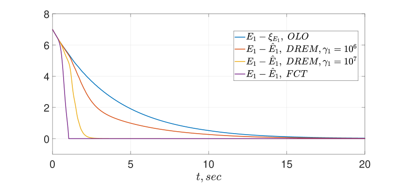
Figure 3: Transients of the first voltage observation error for the OLO (LABEL:dotxi), DREM and FCT-DREM observers with a 30% load change a $t=10$ sec

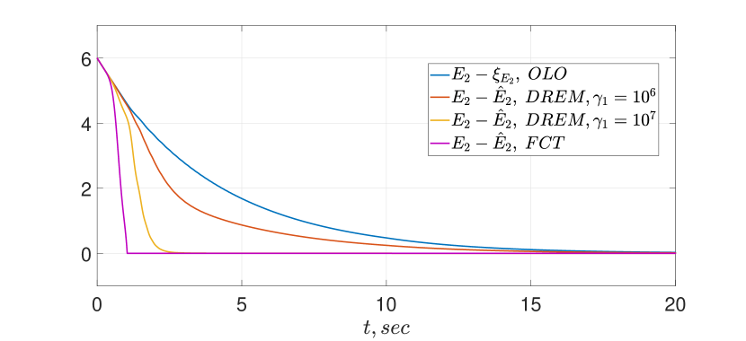
Figure 4: Transients of the second voltage observation error for the OLO (LABEL:dotxi), DREM and FCT-DREM observers with a 30% load change at $t=10$ sec

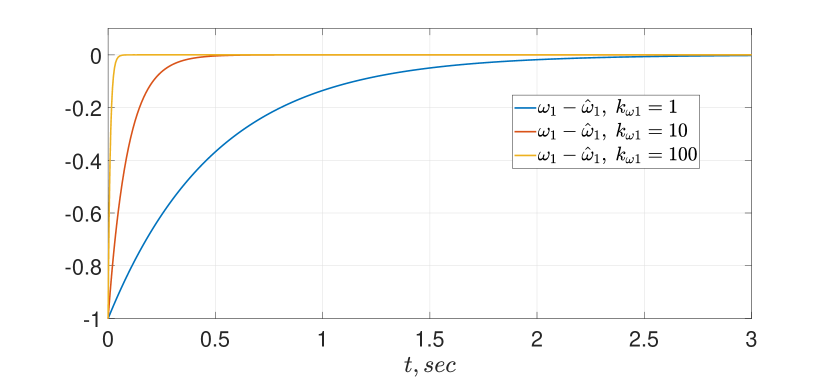
Figure 5: Transients of the first speed observation error for the observer (LABEL:hat_om) for different values of $k_{w1}$

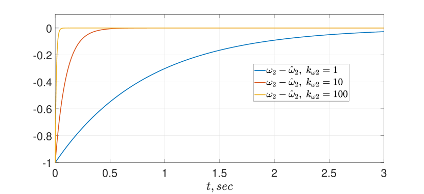
Figure 6: Transients of the second speed observation error for the observer (LABEL:hat_om) for different values of $k_{w1}$

5.3 Chemical-biological reactors

We consider reaction systems whose dynamical model is given by [4, Section 1.5] To simplify the notation we partition the vector $c$ as $c=\mbox{col}(y,x)$, and rewrite (LABEL:sysrea) as The two specific growth rates $\mu_{1}$ and $\mu_{2}$ are given by

$$\begin{bmatrix}\mu_{1}(y_{1})\\ \mu_{2}(y_{2})\end{bmatrix}=\begin{bmatrix}\frac{\mu_{m,1}y_{1}}{K_{S,1}+y_{1}}\\ \frac{\mu_{m,2}y_{2}}{K_{S,2}+y_{2}+K_{I}y_{2}^{2}}\end{bmatrix}.$$

where $\mu_{m,1}$, $\mu_{m,2}$, $K_{S,1}$, $K_{S,2}$ and $K_{I}$ are yield positive coefficients. Notice that $K_{y}$ is square and full rank, consequently

$$y^{\dagger}=K_{y}^{-1}y=-\begin{bmatrix}{y_{1}\over k_{3}}\\ {y_{2}\over k_{1}}+{k_{4}y_{1}\over k_{1}k_{3}}\end{bmatrix}.$$

To design the observer we first identify the signals (LABEL:philamb) of Lemma LABEL:lem2 as Consequently, (LABEL:dotxi) and (LABEL:dotphi) become For the simulations we used the parameters of [17], that is, $k_{1}=268$ mmol/g, $k_{3}=42.14$, $k_{4}=116.5$ mmol/g, $\alpha=1$, $\mu_{m,1}=1.2$ $d^{-1}$, $K_{S,1}=8.85$ g/l, $\mu_{m,2}=0.74$ $d^{-1}$, $K_{S,2}=23.2$ mmol, $K_{I}=0.0039$ mmol^-1, $S_{1,0}=1$, $S_{2,0}=1$ and $u=0.1$. The initial conditions for the anaerobic digester were set to $x_{1}(0)=0.1$ g/l, $y_{1}(0)=0.05$ g/l, $x_{2}(0)=0.5$ g and $y_{2}(0)=4$ mmol/l. We used $\lambda=100$ in the filters of (LABEL:ydotpsi). Fig. 7 and Fig. 8 show the transient behavior of the state estimation errors for different values of the adaptation gain, with $\gamma=0$ corresponding to the OLO. Notice that, although the convergence rate is increased with larger $\gamma$, an undesirable peak appears at the beginning of the error transient.

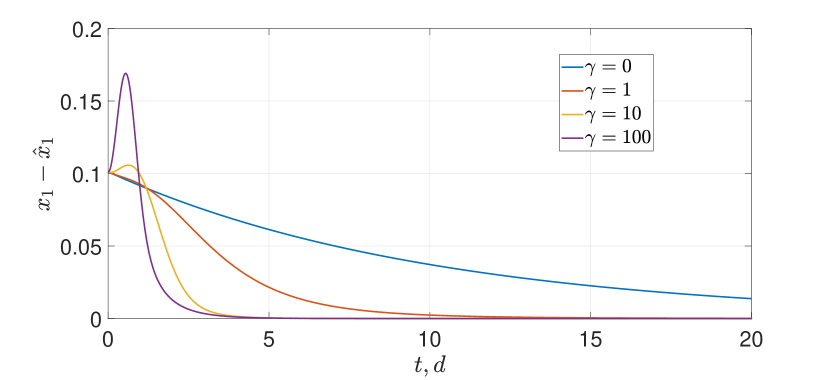
Figure 7: Transients of the error $x_{1}-\hat{x}_{1}$

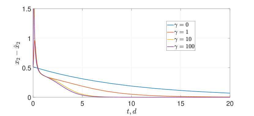
Figure 8: Transients of the error $x_{2}-\hat{x}_{2}$

6 Concluding Remarks

An extension to the PEBO technique reported in [20] has been proposed in the paper. It allows us to simplify the task of solving the key PDE and avoid a, sometimes problematic, open-loop integration required in PEBO. Also, we have identified a condition—verification of the algebraic equation (LABEL:algcon)—that trivializes the task of estimating the unknown parameters. In the original version of PEBO this was left as an open problem to be solved. It is shown that this condition is satisfied for the practically important problem of power systems. It has been shown that combining PEBO with DREM it is possible, on one hand, to relax the excitation conditions to ensure parameter convergence. On the other hand, it allows us to design an observer with FCT under weak excitation assumptions. As an additional example we show the application of PEBO+DREM to reaction systems. Notice that the use of DREM is necessary to solve the parameter estimation problem in this example. Although there are many ways to design an estimator from the linear regression (LABEL:vecreg), there exists a fundamental obstacle to ensure its convergence. Indeed, from the definition of $\Phi_{\Lambda}$, that is $\dot{\Phi}_{\Lambda}=-u\Phi_{\Lambda}$ with $u(t)>0$, we have that $\Phi_{\Lambda}(t)\to 0$, hence $\Psi(t)\to 0$—loosing identifiability of the parameter $\theta$. In particular the matrix $\Psi$ cannot satisfy the well-known persistency of excitation condition

$$\int_{t}^{t+\kappa}\Psi^{\top}(s)\Psi(s)ds\geq\kappa I_{d},$$

which is the necessary and sufficient condition for exponential convergence of the classical gradient and least-squares estimators [27, Theorem 2.5.1].

Appendix A Proof of Proposition 1

From (LABEL:pde) we have that

$$\dot{\phi}=\Lambda\phi+B.$$

Hence, defining the error signal

$$e:=\phi-\xi$$ (13nan)

and taking into account the $\xi$ dynamics of the observer, we obtain an LTV system $\dot{e}=A(t)e$ where we defined $A(t):=\Lambda(u(t),y(t))$. Now, from the (LABEL:dotphi) we see that $\Phi$ is the fundamental matrix of the $e$ system, which is bounded in view of condition (iv). Consequently, there exists a constant vector $\theta\in\mathbb{R}^{n}$ such that

$$e=\Phi\theta,$$

namely $\theta=e(0)$. We now have the following chain of implications

where we have used the fact that for any, possibly singular, $n\times n$ matrix $K$ we have $\mbox{adj}\{K\}K=\det\{K\}I_{n}$ in the last line.

From $\phi=\xi+\Phi\theta$ and (LABEL:phil) it is clear that, if $\theta$ is known, we have that

$$x=\phi^{\mathtt{L}}(\xi+\Phi\theta,y).$$ (13nao)

Hence, the remaining task is to generate an estimate for $\theta$, denoted $\hat{\theta}$, to obtain the observed state via $\hat{x}=\phi^{\mathtt{L}}(\xi+\Phi\hat{\theta},y)$. This is, precisely, generated with (LABEL:gpebo), whose error equation is of the form

$$\dot{\tilde{\theta}}=-\gamma\Delta^{2}\tilde{\theta},$$ (13nap)

where ${\tilde{\theta}}:=\hat{\theta}-\theta$. The solution of this equation is given by

$${\tilde{\theta}}(t)=e^{-\gamma\int_{0}^{t}\Delta^{2}(s)ds}\tilde{\theta}(0).$$ (13naq)

Given the standing assumption on $\Delta$ we have that $\tilde{\theta}(t)\to 0$. Hence, invoking (LABEL:hatx) and (13nao) we conclude that $\tilde{x}(t)\to 0$, where ${\tilde{x}}:=\hat{x}-x$.

Appendix B Proof of Proposition LABEL:pro2

First, notice that the definition of $w_{c}$ ensures that $\hat{x}$, given in (LABEL:ftcgpebo), is well-defined. Now, from (13naq) and the definition of $w$ we have that

$$\tilde{\theta}=w\tilde{\theta}(0).$$

Clearly, this is equivalent to

$$(1-w)\theta=\hat{\theta}-w\hat{\theta}(0).$$

On the other hand, under Assumption LABEL:ass1, we have that $w_{c}(t)=w(t),\;\forall t\geq t_{c}$. Consequently, we conclude that

$${1\over 1-w_{c}}[\hat{\theta}-w_{c}\hat{\theta}(0)]=\theta,\;\forall t\geq t_{c}.$$

Replacing this identity in (LABEL:ftcgpebo) completes the proof.

Appendix C Parameters of the Power System Example

Parameter	Initial values	After load change
$Y_{12}$	0.1032	0.1032
$Y_{21}$	0.1032	0.1032
$b_{1}$	0.0223	0.02236
$b_{2}$	0.0265	0.0265
$D_{1}$	1	1
$D_{2}$	0.2	0.2
$\nu_{1}$	1	1
$\nu_{2}$	1	1
$B_{11}$	-0.4373	-0.5685
$B_{22}$	-0.4294	-0.5582
$G_{11}$	0.0966	0.1256
$G_{22}$	0.0926	0.1204
$a_{1}$	0.2614	0.2898
$a_{2}$	0.2532	0.2864
$P_{1}$	28.22	28.22
$P_{2}$	28.22	28.22
$E_{f1}$	0.2405	0.2405
$E_{f2}$	0.2405	0.2405

References

- [1] Vincent Andrieu and Laurent Praly. On the existence of a kazantzis–kravaris/luenberger observer. SIAM Journal on Control and Optimization, 45(2):432–456, 2006.
- [2] Stanislav Aranovskiy, Alexey Bobtsov, Romeo Ortega, and Anton Pyrkin. Performance enhancement of parameter estimators via dynamic regressor extension and mixing. IEEE Transactions on Automatic Control, 62(7):3546–3550, 2017.
- [3] Alessandro Astolfi, Dimitrios Karagiannis, and Romeo Ortega. Nonlinear and adaptive control with applications. Springer Science & Business Media, 2007.
- [4] George Bastin and Denis Dochain. On-line estimation and adaptive control of bioreactors: Elsevier, amsterdam, 1990 (isbn 0-444-88430-0)., 1991.
- [5] Pauline Bernard. Observer design for nonlinear systems, volume 479. Springer, 2019.
- [6] Pauline Bernard and Vincent Andrieu. Luenberger observers for nonautonomous nonlinear systems. IEEE Transactions on Automatic Control, 64(1):270–281, 2018.
- [7] Gildas Besançon. Nonlinear observers and applications, volume 363. Springer, 2007.
- [8] Denis Dochain. Automatic control of bioprocesses. John Wiley & Sons, 2013.
- [9] Nikolaos Kazantzis and Costas Kravaris. Nonlinear observer design using lyapunov′s auxiliary theorem. Systems and Control Letters, 34(5):241–247, 1998.
- [10] Hassan K. Khalil. High Gain Observers in Nonlinear Feedback Control. SIAM Publishers, 2017.
- [11] Gerhard Kreisselmeier. Adaptive observers with exponential rate of convergence. IEEE transactions on automatic control, 22(1):2–8, 1977.
- [12] Gerhard Kreisselmeier and Gudrun Rietze-Augst. Richness and excitation on an interval-with application to continuous-time adaptive control. IEEE transactions on automatic control, 35(2):165–171, 1990.
- [13] Abhinav Kumar and Bikash Pal. Dynamic Estimation and Control of Power Systems. Academic Press, 2018.
- [14] Prabha Kundur, Neal J. Balu, and Mark G. Lauby. Power system stability and control, volume 7. McGraw-hill New York, 1994.
- [15] Ljung Lennart. System Identification: Theory for the User. Prentice Hall, New Jersey, USA, 1987.
- [16] David Luenberger. Observers for multivariable systems. IEEE Transactions on Automatic Control, 11(2):190–197, 1966.
- [17] Nikolas Marcos, Martin Guay, Denis Dochain, and Tao Zhang. Adaptive extremum-seeking control of a continuous stirred tank bioreactor with haldane’s kinetics. Journal of Process Control, 14(3):317–328, 2004.
- [18] Romeo Ortega, Stanislav Aranovskiy, Anton A Pyrkin, Alessandro Astolfi, and Alexey A Bobtsov. New results on parameter estimation via dynamic regressor extension and mixing: Continuous and discrete-time cases. arXiv preprint arXiv:1908.05125, 2019.
- [19] Romeo Ortega, Alexey Bobtsov, Denis Dochain, and Nikolay Nikolaev. State observers for reaction systems with improved convergence rates. Journal of Process Control, 83:53–62, 2019.
- [20] Romeo Ortega, Alexey Bobtsov, Anton Pyrkin, and Stanislav Aranovskiy. A parameter estimation approach to state observation of nonlinear systems. Systems & Control Letters, 85:84–94, 2015.
- [21] Romeo Ortega, Martha Galaz, Alessandro Astolfi, Yuanzhang Sun, and Tielong Shen. Transient stabilization of multimachine power systems with nontrivial transfer conductances. IEEE Transactions on Automatic Control, 50(1):60–75, 2005.
- [22] Romeo Ortega, Dmitry N. Gerasimov, Nikita E. Barabanov, and Vladimir O. Nikiforov. Adaptive control of linear multivariable systems using dynamic regressor extension and mixing estimators: removing the high-frequency gain assumptions. Automatica, 2019.
- [23] Romeo Ortega, Laurent Praly, Stanislav Aranovskiy, Bowen Yi, and Weidong Zhang. On dynamic regressor extension and mixing parameter estimators: Two luenberger observers interpretations. Automatica, 95:548–551, 2018.
- [24] Anton Pyrkin, Alexey Bobtsov, Romeo Ortega, Alexei Vedyakov, and Stanislas Aranovskiy. Adaptive state observer design using dynamic regressor extension and mixing. Systems and Control Letters, 133:1–8, 2019.
- [25] Anton A. Pyrkin, Alexey A. Vedyakov, Romeo Ortega, and Alexey A. Bobtsov. A robust adaptive flux observer for a class of electromechanical systems. International Journal of Control, pages 1–11, 2018.
- [26] Wilson Rugh. Linear Systems Theory. Prentice Hall, NJ, USA, 1996.
- [27] Shankar Sastry and Marc Bodson. Adaptive Control: Stability, Convergence and Robustness. Prentice Hall, New Jersey, USA, 1989.
- [28] Peter W. Sauer, Mangalore A. Pai, and Joe H. Chow. Power system dynamics and stability: with synchrophasor measurement and power system toolbox. John Wiley & Sons, 2017.
- [29] Bowen Yi, Romeo Ortega, and Weidong Zhang. On state observers for nonlinear systems: A new design and a unifying framework. IEEE Transactions on Automatic Control, 64(3):1193–1200, 2018.