Orbital Parameter Determination for Wide Stellar Binary Systems in the Age of Gaia

Abstract

The orbits of binary stars and planets, particularly eccentricities and inclinations, encode the angular momentum within these systems. Within stellar multiple systems, the magnitude and (mis)alignment of angular momentum vectors among stars, disks, and planets probes the complex dynamical processes guiding their formation and evolution. The accuracy of the Gaia catalog can be exploited to enable comparison of binary orbits with known planet or disk inclinations without costly long-term astrometric campaigns. We show that Gaia astrometry can place meaningful limits on orbital elements in cases with reliable astrometry, and discuss metrics for assessing the reliability of Gaia DR2 solutions for orbit fitting. We demonstrate our method by determining orbital elements for three systems (DS Tuc AB, GK/GI Tau, and Kepler-25/KOI-1803) using Gaia astrometry alone. We show that DS Tuc AB’s orbit is nearly aligned with the orbit of DS Tuc Ab, GK/GI Tau’s orbit might be misaligned with their respective protoplanetary disks, and the Kepler-25/KOI-1803 orbit is not aligned with either component’s transiting planetary system. We also demonstrate cases where Gaia astrometry alone fails to provide useful constraints on orbital elements. To enable broader application of this technique, we introduce the python tool lofti_gaiaDR2 to allow users to easily determine orbital element posteriors.

1 Introduction

The monitoring of orbits is one of the oldest tools used to measure the properties and evolution of astrophysical systems. Orbital periods and semi-major axes convey the masses of systems, and have been used to weigh the universe in the context of planets (Christy & Harrington 1978), stars (Aitken, 1918), and galaxies and their dark matter halos (Rubin & Ford 1970). However, a broad range of astrophysical effects can also be probed using the other orbital elements– eccentricities and orientations–that encode information about the magnitude and direction of the angular momentum vector(s) in a system. Even in its simplest form, much can be inferred about a system’s formation and past history by the relative (mis)alignment of angular momentum vectors for different objects and on different scales.

On the scale of stellar systems (single or multiple) and their attendant planetary systems, angular momentum vectors trace their condensation out of interstellar clouds, and their subsequent orbital evolution through N-body interactions. In the classical picture of star formation, the collapse of a spherical protostellar core forms a central star whose rotation, circumstellar disk, and natal planetary system are aligned with the initial angular momentum of the primordial core (e.g., Shu et al. 1987). However, asymmetry in the mass distribution and gas motions of protostellar cores can be driven by phenomena like turbulence and magnetic fields, which complicate this simple picture of angular momentum evolution. (e.g., Boss & Bodenheimer, 1979; Lee et al., 2019).

These same effects are thought to be the main drivers of wide ($a\gtrsim 50$ AU; Duchêne & Kraus 2013; Moe & Di Stefano 2017) binary star formation in the core fragmentation scenario (Burkert & Bodenheimer, 1993; Bate, 2000; Offner et al., 2010, 2016), which must operate broadly to account for the observed ubiquity of binary and higher order systems at these separations (e.g., Duquennoy & Mayor, 1991; Raghavan et al., 2010; Kraus et al., 2008, 2011). The subsequent evolution of protoplanetary disks in the binary environment can be perturbed from their initial configuration by torques from the companion (Papaloizou & Terquem, 1995; Batygin, 2012; Lai, 2014), while also dampening misalignment of orbiting bodies (Goldreich & Tremaine, 1980; Artymowicz, 1992). These complex dynamical interactions can destroy or re-introduce alignment between planetary systems, binary orbits, and stellar rotation. Additionally, binaries on scales with $a\lesssim 100$ AU can also be formed via disk fragmentation, which would be expected to form well aligned systems (Tobin et al., 2016; Tokovinin & Moe, 2019). Finally, discrete objects within the system can interact through long-term secular effects (e.g., Kozai, 1962; Lidov, 1962; Fabrycky & Tremaine, 2007) or strong scattering via three-body interactions (Rasio & Ford, 1996; Weidenschilling & Marzari, 1996; Bate et al., 2002; Chatterjee et al., 2008) to exchange orbital energy and angular momentum, driving the evolution and randomization of angular momentum vectors.

There is extensive observational evidence for both alignment and misalignment among the stars, disks, and planets in binary systems. In the case of stellar properties, measurements for close systems ($a\lesssim 50$ AU) suggest broad alignment of stellar spin (Hale, 1994) and binary orbits (Tokovinin & Latham, 2017), as well as for inner and outer orbits of hierarchical, high-order multiple systems (Tokovinin, 2018a). In contrast, very wide systems do not show any correlation, though the ability to conduct this measurement is still quite new (e.g., Tokovinin, 2018b). Protoplanetary disks within young binary systems are seen in both states (mis-/aligned) with respect to each other (Stapelfeldt et al. 1998; Jensen et al. 2004) and the binary orbit (Winn et al. 2004; Plavchan et al. 2013; Schaefer et al. 2014). In systems which host circumbinary disks, binaries with $a\lesssim$ 1 AU exhibit tight alignment between the binary orbit and the disk plane, while systems with wider separations appear to have a random distribution of mutual inclinations (Czekala et al., 2019). The first orbital motion measurements for planet-hosting wide binaries rule out a random distribution of planet-binary mutual inclinations, showing that while the alignment might not be as strongly correlated as for multi-planet systems ($\lesssim 5\arcdeg$; Lissauer et al. 2011), they tend towards alignment rather than random orientations with respect to the planets (e.g., Dupuy et al. 2016; Dupuy et al., in prep).

The emerging trend from these studies is that the alignment between system components appears to increase with decreasing separation. This may be the effect of dynamical processes that align systems more efficiently at small separations, or a signpost for their formation process. In the case of planets, for instance, occurrence rates of protoplanetary disks and transiting planets are seen to decline for binary systems with separations less than $\sim$50 AU (Kraus et al., 2012, 2016). Given the results above, this absence might suggest that mutual alignment is a condition for the systems (disk or planetary) that do survive. Testing this hypothesis, as well as determining the relevant scales where alignment becomes common/necessary (which appears to differ depending on the subsystem; binary-triple orbits, stellar rotation axes, binary-planetary orbits, etc) requires a large population of systems with well-characterized orbital parameters at a various evolutionary stages. While the sample is growing, constraining wide orbit systems is the bottleneck through which all future progress must pass.

For decades there has been extensive effort to accurately determine probable orbits for visual stellar and substellar companion systems using time-series astrometric monitoring (e.g. Heintz, 1978; Kiselev & Kiyaeva, 1980; Ségransan et al., 2000; Benedict et al., 2016; Kiyaeva et al., 2017). These measurements have enabled comparisons with the known inclinations of planets or disks around individual components (e.g. Dupuy et al., 2016; Bryan et al., 2020). The Gaia astrometric revolution presents an opportunity to obtain similarly meaningful constraints on wide stellar binary orbital parameters quickly in comparison. Gaia DR2 (Gaia Collaboration et al., 2016; Gaia Collaboration et al., 2018) already reports precise positions and proper motions for many wide stellar binaries, and future data releases will increase the number of systems (resolving tighter pairs and presenting astrometry for fainter companions) and further improve the measurement uncertainties. The wealth of new systems resolved by Gaia is a boon to statistical studies of binary-disk and binary-planet alignment and permits new analyses of systems for which time series astrometry is not yet available.

As has long been noted for orbit fits, several families of orbit solutions match observations when a small fraction of an orbit is observed (Aitken, 1918). In most cases, Gaia measurements of relative positions and velocities do not provide enough observations to fully determine unique orbit solutions, however in this work we show that they can constrain the orbital elements to a scientifically useful degree. We find that for a range of binary configurations, Gaia DR2 astrometry alone can provide orbital parameter posterior distributions that are consistent with, and in some cases superior to, long time series astrometric observations. We caution that not all binary systems are amenable to this approach, as we discuss in Section 4.

In Section 2, we describe our orbit fitting technique combining Gaia DR2 relative positions and proper motions with the Orbits for the Impatient (OFTI, Blunt et al. 2017) rejection sampling orbit fitting method. We also recommend metrics for assessing the quality of the Gaia solution and accuracy of the technique. In Section 3, we demonstrate the power of this technique by applying it to several binary systems resolved by Gaia DR2. In Section 4, we show how the quality of the Gaia DR2 solution can limit the accuracy of this technique, and illustrate with examples where the technique fails to be as accurate as other methods. In Section 5, we summarize the general classes of systems for which this technique is and is not sufficient, and discuss improvements with future Gaia data releases.

2 Method

There are nine observable parameters describing the motion of one body relative to another — three position ($X$, $Y$, $Z$), velocity ($\dot{X}$, $\dot{Y}$, $\dot{Z}$), and acceleration ($\ddot{X}$, $\ddot{Y}$, $\ddot{Z}$) terms, where $X$ and $Y$ define the plane of the sky. Seven parameters are required to describe a Keplerian orbit in three dimensions — semi-major axis ($a$), orbital period ($P$), eccentricity ($e$), inclination ($i$), argument of periastron ($\omega$), position angle of nodes ($\Omega$), and time of periastron passage ($T_{0}$). If the total system mass is known, providing orbital period, then six independent measurements of the orbit are needed to obtain a unique orbit solution. Traditional orbit determinations using time series astrometric measurements encode velocity and acceleration information in the time series data, and when a significant fraction of the orbit is observed, a unique orbit solution can be obtained. Gaia DR2 was obtained using time-series astrometry, but the catalog reports the binary relative $\Delta$RA ($\Delta\alpha$, corresponding to $Y$), $\Delta$DEC ($\Delta\delta$, $X$), proper motion in RA/DEC ($\Delta\mu_{\alpha}$, $\dot{Y}$), $\Delta\mu_{\delta}$ $\dot{X}$), and in some cases radial velocity ($\Delta$RV, $\dot{Z}$) at a single epoch (2015.5 for Data Release 2; Lindegren et al. 2018). Thus four net observations, $X$, $Y$, $\dot{X}$, $\dot{Y}$, (or five, adding $\dot{Z}$ if radial velocities for both sources are present) can be used to constrain the orbit parameters at a single time point for a stellar binary for which both members are resolved by Gaia. Gaia parallaxes are not precise enough to constrain line of sight position ($Z$).

The measurements reported in Gaia DR2 will not be sufficient to fully determine an orbit, and instead deliver a family of orbital solutions. In spite of this, we show in Section 3 that the orbital constraints from Gaia can provide meaningful insight into system dynamics. The additional measurements reported in future data releases (such as acceleration terms) will further restrict those orbital solutions and increase the power of this technique; we describe the mathematical additions required to harness these acceleration measurements in Appendix A.3.

2.1 Orbit fitting method

The intent of this work is to examine the suitability of Gaia astrometry as the sole measurement for constraining orbital elements of wide binaries. Any method of orbit fitting can be adapted to accommodate Gaia position and velocity measurements. In this work, we have chosen to adapt the Orbits for the Impatient (OFTI, Blunt et al., 2017) rejection sampling algorithm to make use of the Gaia astrometry.

Previously, OFTI has been used to compare astrometric observations, either separation/position angle (PA) or RA/DEC, at several observation epochs separated in time to predicted observations for trial orbits (Blunt et al. 2017, Pearce et al. 2019). Here we adapt OFTI to fit the linear plane-of-sky velocity vector provided by Gaia DR2, and adopted the name LOFTI (Linear OFTI) for this application.

Rather than time-series observations, our modified OFTI uses relative $\Delta\alpha$, $\Delta\delta$, relative proper motions ($\Delta\mu_{\alpha}$, $\Delta\mu_{\delta}$), and $\Delta$RV if available, at the single Gaia DR2 epoch (2015.5) to constrain orbital parameters. Here $\Delta\mu_{\alpha}$ is chosen to be $\Delta\mu_{\alpha}$ = $\Delta\mu_{\alpha,sec}~{}-~{}\Delta\mu_{\alpha,pri}$, likewise $\Delta\alpha$, $\Delta\delta$, $\Delta\mu_{\delta}$ and $\Delta$RV.

The OFTI method is described in detail in Blunt et al. (2017), but we summarize briefly here. OFTI is a rejection sampling algorithm that randomly generates four orbital parameters from uniform priors for eccentricity (e), argument of periastron ($\omega$), mean anomaly from which we derive epoch of periastron passage (t₀), and cosine of inclination cos(i). We assume the total system mass from prior measurements in the literature (typically based on previous temperature and luminosity measurements) and utilize the Gaia parallax in order to remove orbital period as a free parameter via Kepler’s 3rd law. The semi-major axis (a) and longitude angle of ascending node ($\Omega$) for all trial orbits are scaled and rotated from an arbitrary initial value to match the Gaia $\Delta\alpha$ and $\Delta\delta$ positions. The scale-and-rotate step speeds up the rejection sampling process by avoiding the large majority of potential orbits with extremely discrepant separations or PAs, and means that for our six-dimensional parameter space, we have only four free parameters. After scale-and-rotate, we compute the relative velocities of each trial orbit at the observation date, and perform a rejection sampling accept/reject decision, in which an orbit is accepted if its probability is larger than a randomly chosen number from the interval [0,1]. The probability of a trial orbit is given as P$(trial\;orbit|observations)=e^{-\frac{\chi^{2}}{2}}$ where

$$\chi^{2}=\big{(}\frac{\Delta\mu_{\alpha}-\dot{Y}}{\sigma_{\mu_{\alpha}}}\big{)}^{2}+\big{(}\frac{\Delta\mu_{\delta}-\dot{X}}{\sigma_{\mu_{\delta}}}\big{)}^{2}$$ (1)

$X$, $Y$, $\dot{X}$, and $\dot{Y}$ denote predictions from trial orbits, while $\alpha,\,\delta,\,\mu_{\alpha},\,\mu_{\delta}$ denote observations from Gaia. An additional radial velocity term can be added to the $\chi^{2}$ if applicable.

OFTI is particularly well-suited for poorly constrained orbital motion, such as long-period systems with astrometry for only a small orbit fraction, and is able to quickly determine orbital element posteriors for systems where Markov Chain Monte Carlo (MCMC) might not converge (Blunt et al. 2017, Blunt et al. 2019). However, it can be prohibitively slow when the orbit is well-constrained because the majority of trials will be rejected due to low probability (Blunt et al. 2019). Future Gaia data releases will include more systems with well-determined radial velocities ($\dot{Z}$), and accelerations in the plane of the sky ($\ddot{X}$, $\ddot{Y}$), further constraining the orbit. If more constraints are added, the orbit fit would be better served by another fitting method such as MCMC. However, even in this case OFTI is still useful in narrowing the parameter space and determining a starting point for an MCMC.

The accuracy of OFTI depends on the accuracy of the astrometric observations and their assessed uncertainties, which we discuss in the following section. Furthermore, while OFTI fully samples the parameter space, the posteriors will still be subject to degeneracies among orbital parameters. Some pathological orbits, or orbits observed at pathological times, might be subject to irreducible degeneracies even in the case where the data are accurate and precise. For example, when the motion is purely along the separation direction, it can be difficult without additional information to distinguish between an edge-on orbit and a highly eccentric orbit. Finally, the need to estimate component stellar masses will introduce a dependence on stellar evolutionary models and external data sources, with all of the associated uncertainties associated with both. There may also be cases where systematic errors can emerge, such as when unidentified additional stellar components within the system contribute additional mass that is not incorporated into the model. These risks must be assessed on a case-by-case basis, but if they can be reduced to an acceptable level, then LOFTI provides a powerful tool for many astrophysical applications.

To allow users to easily and quickly implement this technique, we provide the simple python package lofti_gaiaDR2. The GitHub repository includes documentation and examples for implementing this code, and Appendix 2 briefly describes the python tool.

2.2 Data Quality Indicators

For any astrometric orbit-fitting technique, the utility and accuracy of the orbital solution will depend on the accuracy and precision of the observations. For Gaia measurements, there are many potential quality indicators for a given solution (Lindegren et al., 2018; Lindegren, 2018), but the most complete indicator is the re-normalized unit weight error (RUWE) (Lindegren, 2018). In brief, RUWE is the square root of the reduced $\chi^{2}$ statistic, corrected for its dependence on color and magnitude. It can be computed using methods described in Lindegren (2018), or found in the table gaiadr2.ruwe of the Gaia archive. RUWE close to 1.0 indicates that the single star model is a good fit to observations; higher RUWE, such as RUWE $>$ 1.4, are typically found to be spatially resolved binaries with compromised astrometric accuracy (e.g. Rizzuto et al., 2018; Ziegler et al., 2019).

Other useful metrics are available in the Gaia DR2 catalog and discussed in the Gaia DR2 documentation.

Table 1: Selected Gaia binaries and their input parameters

Name	Mass	G mag	Parallax	RUWE	Separation [mas]	Velocityj	WDS ID
Gaia DR2 Source ID	[M⊙]	[mag]	[mas]		P.A. [deg]	[km s-1]	(if applicable)
DS Tuc A	1.01$\pm$0.06a	8.32	22.666 $\pm$ 0.035	1.034	5364.61$\pm$0.03	1.94$\pm$0.72k	23397-6912
6387058411482257536
DS Tuc B	0.84$\pm$0.06a	9.40	22.650 $\pm$ 0.029	1.015	347.6582$\pm$0.0002
6387058411482257280
GK Tau	0.79$\pm$0.07b	11.88	7.7362 $\pm$ 0.0434	1.089	13157.97$\pm$0.05	1.15$\pm$0.11	…
147790206908395776
GI Tau	0.53${}^{+0.09\,c}_{-0.11}$	12.70	7.6625 $\pm$ 0.0460	1.046	328.4399$\pm$0.0002
147790202612482560
Kepler-25	1.159${}^{+0.040\,d}_{-0.051}$	10.63	4.082 $\pm$ 0.024	0.998	8415.29$\pm$0.02	0.879$\pm$0.081	…
2100451630105041152
KOI-1803	0.794$\pm$0.026e	13.24	4.089 $\pm$ 0.014	1.060	288.2891$\pm$0.0002
2100451630105040256
Gl 896 A	0.3880$\pm$0.0091f	9.04	159.710 $\pm$ 0.082	1.173	5380.71$\pm$0.09	2.477$\pm$0.009	23317+1956
2824770686019003904
Gl 896 B	0.2519$\pm$0.0076f	10.82	160.060 $\pm$ 0.108	1.460	78.0372$\pm$0.0008
2824770686019004032
Kepler-444 A	0.76$\pm$0.04g	8.64	27.414 $\pm$ 0.029	1.000	1837.44$\pm$0.34	2.39$\pm$0.24	…
2101486923385239808
Kepler-444 BC	0.54$\pm$0.04h	12.27	32.652 $\pm$ 0.569	16.687	252.76$\pm$0.02
2101486923382009472
RW Aurigae A	1.20$\pm$0.24i	11.11	6.1157 $\pm$ 0.067	1.774	1488.63$\pm$0.66	2.25$\pm$1.18	…
156430822114424576
RW Aurigae B	0.72$\pm$0.14i	11.40	6.583 $\pm$ 0.902	28.904	74.47$\pm$0.03
156430817820015232

Note. — All input parameters derived from Gaia astrometry, and given as the second component relative to the first component. (a) Newton et al. 2019, (b) Kenyon & Hartmann 1995, (c) Akeson et al. 2019, (d) Silva Aguirre et al. 2015, (e) Fulton & Petigura 2018, (f) this work, via the mass-luminosity relation of Mann et al. 2019 and 2MASS K-band magnitudes, (g) Campante et al. 2015, (h) Dupuy et al. 2016, (i) Kraus et al. 2011, (j) Velocity in the plane of the sky, given as $v=\sqrt{\mu_{\alpha}^{2}+\mu_{\delta}^{2}}$  (k) DS Tuc relative velocity includes radial velocity.

3 Validation demonstrated by successful fits

To assess the validity of the fitting method, we tested if a fit constrained by Gaia astrometry would return the same posterior distribution as a multi-epoch astrometric OFTI fit for a given system (Section 3.1), and applied this technique to new interesting systems (Section 3.2 and 3.3). Table 1 lists the binary systems studied in this and Section 4, and their input parameters derived from Gaia astrometry.

Table 2: Summary of Orbital Parameters for DS Tuc AB

	Astrometry-Only						Gaia Position/Velocity-Only
Element	Median	Std Dev	Mode	68.3% Min CI	95.4% Min CI		Median	Std Dev	Mode	68.3% Min CI	95.4% Min CI
log($a$) (AU)	2.35	0.30	2.38	(2.08, 2.47)	(2.08, 3.12)		2.28	0.21	2.21	(2.19, 2.36)	(2.19, 2.80)
$e$	0.63	0.29	0.99	(0.50, 0.99)	(0.09, 0.99)		0.57	0.10	0.47	(0.46, 0.60)	(0.46, 0.77)
$i$ (°)	98.2	11.4	93.3	(90.1, 98.1)	(86.8, 126.2)		96.9	0.9	96.6	(96.0, 97.8)	(95.0, 98.6)
$\omega$ (°)	6	103	302	(-71, 156)	(-160, 180)		6	35	36	(340, 52)	(297, 62)
$\Omega$ (°)	66	95	348	(-15, 168)	(-36, 179)		167	16	167	(164, 170)	(163, 174)
$T_{0}$ (yr)	-2380	32970	1400	(140, 1640)	(-13160, 2015)		1250	480	1520	(1250, 1530)	(-590, 1530)
log(Periastron) (AU)	1.90	0.79	2.35	(1.13, 2.41)	(-0.09, 3.14)		1.91	0.21	1.94	(1.73, 2.08)	(1.35, 2.17)

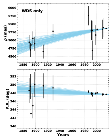
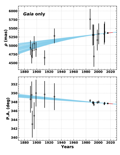
Figure 1: Successful fit: DS Tuc. Left: A selection of 100 orbits for DS Tuc B relative to DS Tuc A from the posterior of orbits, fit using the WDS astrometry points only. The WDS astrometry data are overplotted. Error bars are estimated from root mean square error about two linear fits to separation and position angle independently for the pre-1940 group and the post-1980 group. Scatter, and thus error bars, are not the same in both dimensions, and so systematic error differences exist that are not accounted for in our error estimate. Right: A selection of 100 orbits from the posterior of the fit against Gaia DR2 position, velocities, and radial velocity, with the WDS astrometry overplotted for comparison (open circles, not used in fit). The red line indicates the direction of the Gaia velocity vector. The Gaiaonly fit matches the trend of the WDS-only fit, but is more tightly constrained.

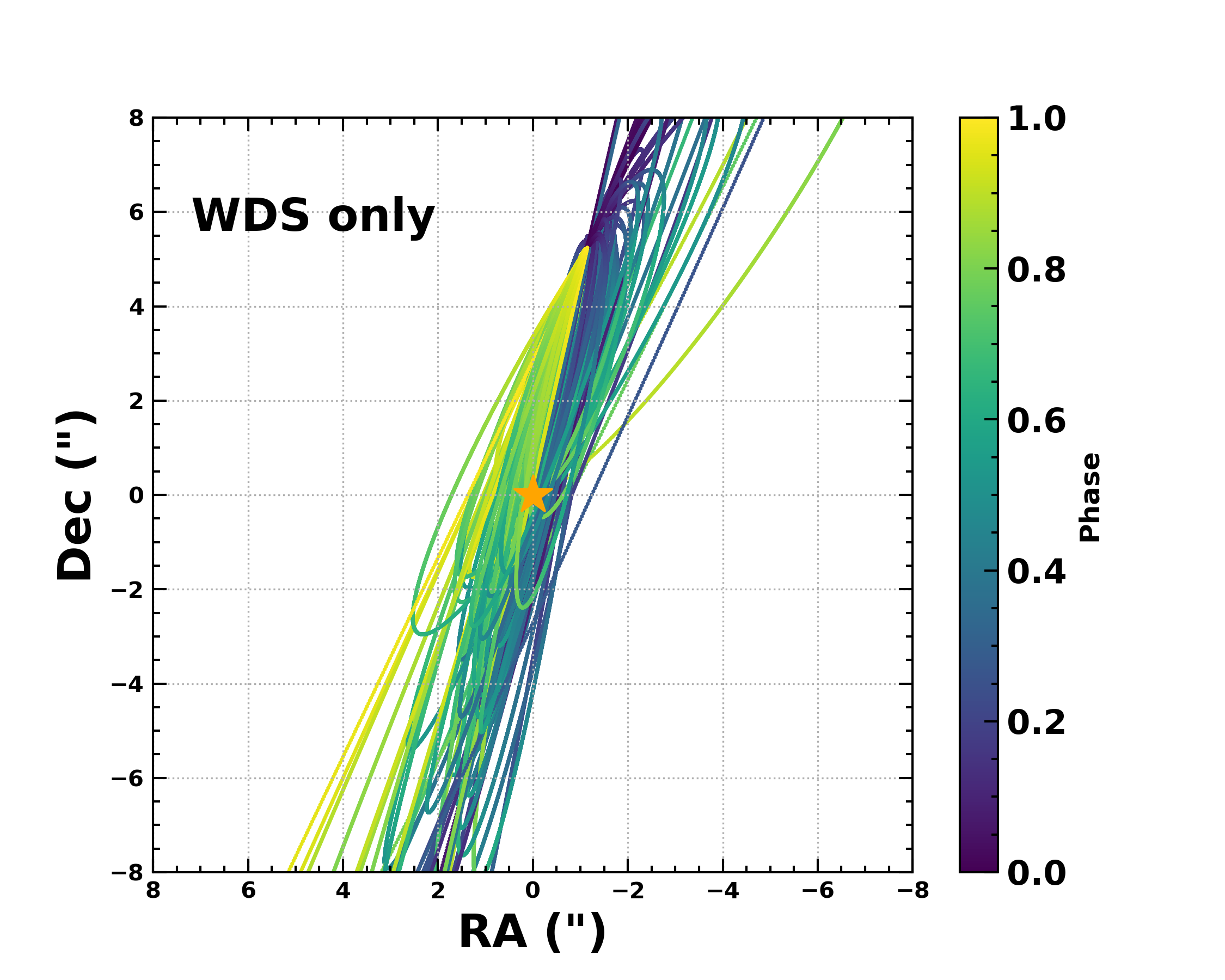
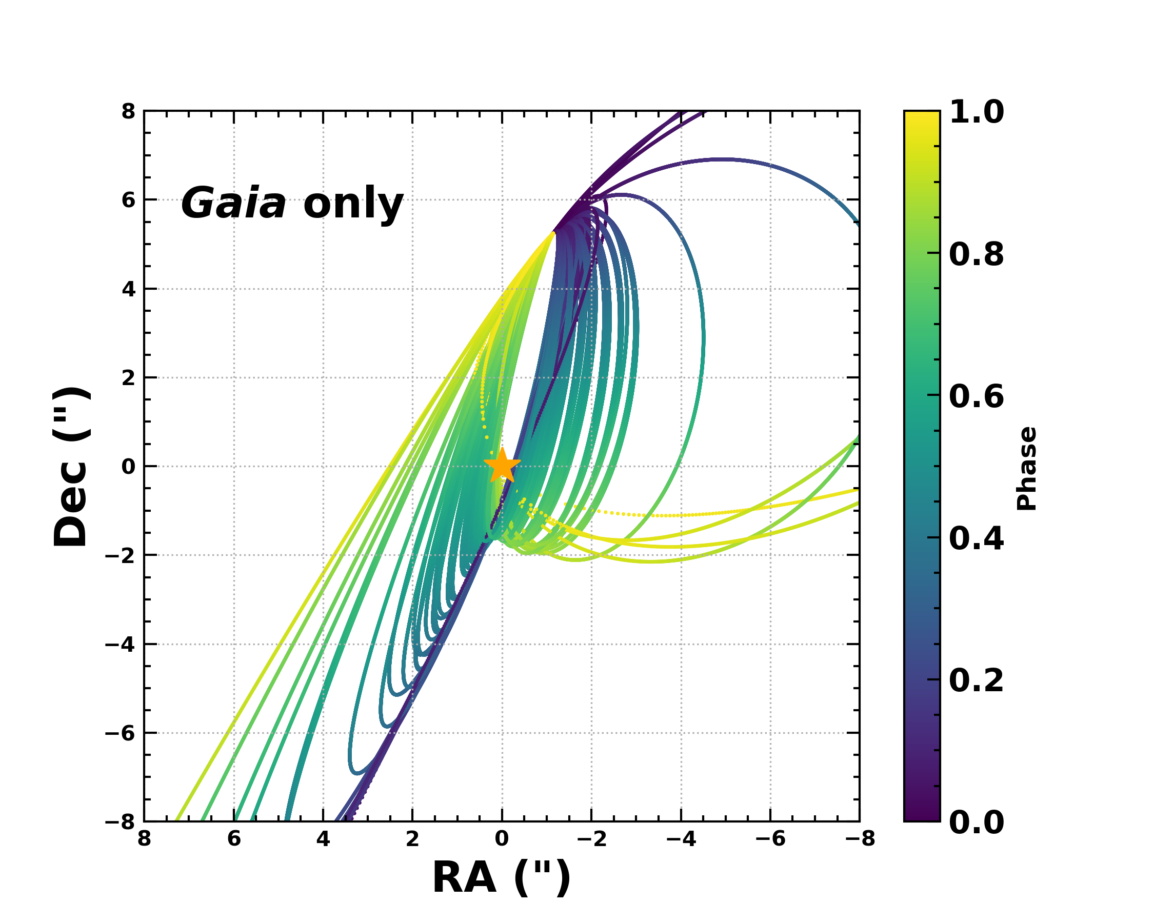
Figure 2: DS Tuc. Left: Selection of 100 orbits for DS Tuc B relative to DS Tuc A from the posterior of orbits fit against the WDS astrometry data only in the plane of the sky. Right: Selection of 100 orbits from the posterior of the fit against Gaia DR2 position, velocities, and radial velocity.

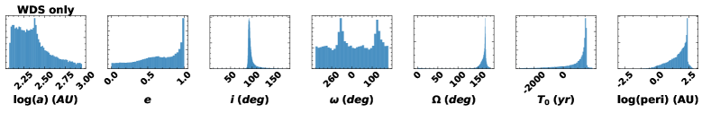
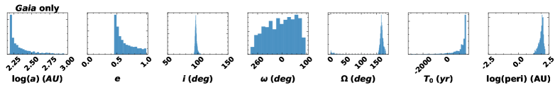
Figure 3: DS Tuc. Top: Histogram of posterior distributions of orbital elements for the WDS astrometry-only OFTI fit. Bottom: Histograms of orbital elements for the Gaia linear velocity fit, including Gaia radial velocities. Semi-major axis (a) and epoch of periastron passage (T₀) have been truncated in both for clarity. The linear fit agrees broadly with the astrometry-only fit, but is much more tightly constrained, and suppresses some of the more extreme orbital solutions, most notably circular and low eccentricity, very high eccentricity, and large semi-major axis orbits.

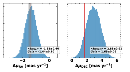
Figure 4: DS Tuc. Posterior distribution of instantaneous orbital velocity in right ascension (left; $\Delta\mu_{\rm{RA}}$) and declination (right; $\Delta\mu_{\rm{DEC}}$) from the long period astrometric (WDS only) DS Tuc orbit fit, with the Gaia DR2 measurements indicated by a red vertical line and grey shading for the uncertainties. The Gaia measurement agrees with the mean of the astrometric posterior in right ascension, and is 1.3-$\sigma$ from the mean of the posterior distribution in declination.

3.1 DS Tuc with WDS and Gaia

The young planet host DS Tuc (HD 222259) is a visual binary (Torres, 1988) with DS Tuc A (Spt = G6V, M_∗ = 1.01 $\pm$ 0.06 M_⊙; Newton et al. 2019) and DS Tuc B (SpT = K3V, M_∗ = 0.84 $\pm$ 0.06 M_⊙; Newton et al. 2019) separated by 5^′′ (Torres et al., 2006). The masses were determined using isochrones by Newton et al. DS Tuc A hosts a transiting planet with a radius of 5.70$\pm$0.17 R_⊕ (Newton et al., 2019). In Newton et al. (2019), we used LOFTI to study the orbital alignment of DS Tuc AB, and found the binary was nearly aligned with the planet orbit. Here we demonstrate how our technique provided a tighter constraint on most orbital elements than time series astrometry alone for this system.

The Washington Double Star (WDS, Mason et al., 2001) Catalog provides separation and position angle measurements for stellar binaries spanning decades. The WDS catalog provides a long time baseline for computing orbits astrometrically, which we verified against orbital posteriors for Gaia DR2 linear velocity orbit fits. WDS data for DS Tuc go back as far as 1870, and both objects have well-defined solutions in Gaia DR2, including radial velocities. We performed an astrometry-only fit to the WDS measurements with standard OFTI, and compared the results to a Gaia LOFTI fit.

Astrometric fit with standard OFTI: We fit orbital parameters to the relative astrometry of DS Tuc AB using the established OFTI method described in Pearce et al. (2019) and Blunt et al. (2017). The WDS astrometry used in the fit is displayed in Figure 1. To establish errors on separation and position angle we used the root-mean-squared error (RMSE) about a linear fit to the WDS astrometry. As can be seen in Figure 1, the observations divide into two groups, an earlier group (before 1940) with more scatter, and a later group (after 1980) with smaller scatter, and so we determined the RMSE about that line for each group independently. The latest data point is the Gaia DR2 measurement, which uses the Gaia reported error.

Gaia position/velocity vector fit: We performed a LOFTI position/velocity vector fit using the relative $\Delta\alpha$, $\Delta\delta$, $\mu_{\alpha}$, $\mu_{\delta}$, and radial velocity reported in Gaia DR2. The Gaia relative radial velocity measurement $\Delta$RV = 1.88$\pm$0.72 km s^-1 agrees with the mean relative radial velocity measurement of $\Delta$RV = 1.64$\pm$0.35 km s^-1 reported by Newton et al. (2019).

The posterior parameters for both fits are given in Table 2. Figures 1 and 2 show a selection of orbits from the astrometric (WDS only, left) and velocity vector (Gaia only, right) fits. Marginal posterior distributions for orbital parameters for each fit are shown in Figure 3.

Figure 1 demonstrates that both fits agree broadly with the astrometric points and display the same general trend, however the linear velocity fit is more tightly constrained. The 1-dimensional orbital element distributions also broadly agree, but the linear velocity fit has suppressed some of the more extreme orbits, namely highly eccentric, larger semi-major axis, and extremely close periastron orbits. Circular and low eccentricity orbits are also ruled out from the Gaia fit.

Finally, Figure 4 displays the posterior distribution of proper motion in RA ($\mu_{\rm{RA}}$) and Dec ($\mu_{\rm{DEC}}$) computed from posterior orbits in the WDS-only fit. The Gaia DR2 proper motions are indicated with a red vertical line. The Gaia measurements are in the posterior of the astrometry-only fit. The mean of the $\mu_{\rm{RA}}$ distribution agrees with Gaia inside of 1$\sigma$, and the $\mu_{\rm{DEC}}$ mean is a little more than 1$\sigma$ from the Gaia measurement. This is likely the source of the differences in parameter posterior distributions between the astrometry and the Gaiaonly fits, with the Gaia measurement being more robust due to small fractional uncertainties.

We conclude from this analysis that for DS Tuc, fitting the Gaia astrometry alone produced a posterior that agrees with, but is more precise than, fitting against time series astrometry alone. Combining the time series astrometry with the Gaia velocities resulted in an even more tightly constrained orbital parameter posterior, which is reported in Newton et al. (2019) and is used in their analysis of this system.

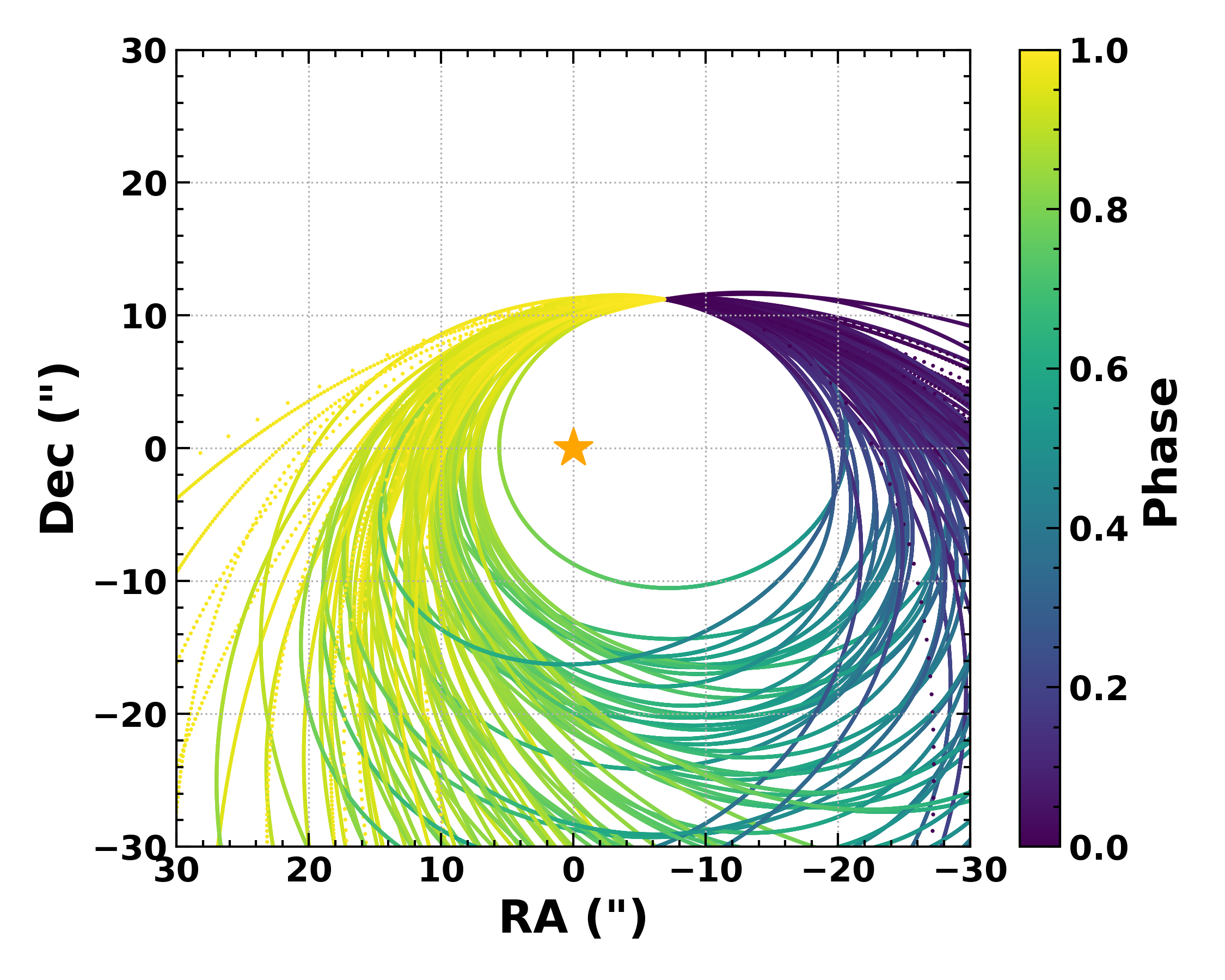
Figure 5: Successful fit: GK/GI Tau. GK Tau hosts a protoplanetary disk with inclination $i=71\pm 5^{\circ}$ or $i=109\pm 5^{\circ}$. The inclination allowed by the Gaia astrometry is limited to 160 ${}^{+13}_{-10}$ degrees at the 68% credible interval. Orbits consistent with GK Tau’s disk inclination are ruled out, and the extent of the disk is far smaller than the closest periastron distances, indicating that the wide binary orbit is not influencing the evolution of the disk. Top: Selection of 100 orbits from the posterior of the LOFTI fit of GI Tau relative to GK Tau. Bottom: Posterior distributions of orbital elements for the Gaia position/velocity fit of GI Tau relative to GK Tau. The long tail of semi-major axis and T₀ has been truncated for clarity.

3.2 GK/GI Tau with Gaia

The Taurus pre-main sequence stars GK Tau (SpT = K7; Kenyon & Hartmann 1995; M = 0.79 $\pm$ 0.07 M_⊙ via dynamical mass; Simon et al. 2017) and GI Tau (SpT = M0.4, M = $0.53^{+0.09}_{-0.11}$ M_⊙ via isochrones; Herczeg & Hillenbrand 2014; Akeson et al. 2019) are a wide separation ($\rho\,=\,$13.2″, or $\rho=1700$ AU) binary system in Taurus (Hartigan et al. 1994; Duchêne et al. 1999; Kraus & Hillenbrand 2009; distance $d\,=\,129.3\pm 0.7$ pc). GI Tau and GK Tau appear to be part of the classically defined Taurus-Auriga star-forming region, with an age of 1–3 Myr (Kraus & Hillenbrand, 2009). Both GK Tau and GI Tau host gas-rich protoplanetary disks.

Long et al. (2019) measure disk inclinations of $i=40.2^{+5.9}_{-6.2}$ deg and $i=43.8\pm 1.1$ deg, and position angles of PA = $119.9^{+8.9}_{-9.1}$ deg and PA = $143.7^{+1.9}_{-1.6}$ deg for GK Tau and GI Tau respectively. The disk inclinations could also be $139.8^{+5.9}_{-6.2}$ deg and $136.2\pm 1.1$ deg, as the reported value uses the convention of $i<90^{\circ}$.

Table 1 shows that Gaia has low RUWE values for GK Tau (RUWE = 1.089), and GI Tau (RUWE = 1.046). GI Tau has a small amount of excess noise with low significance, but the relative velocity is still measured to be non-zero at 10$\sigma$ significance. High resolution imaging has ruled out additional stellar companions to either source down to $\rho\sim 5$ AU (Kraus et al., 2011).

Figure 5 shows the posterior distributions of the orbital elements resulting from our fit to the Gaia position/velocity alone. A binary inclination consistent with either of GK Tau and GI Tau’s possible disk inclinations is marginally consistent with the Gaia astrometry, though most of the orbital inclination posterior is concentrated in more face-on orientations. In the future, a more precise measurement of the relative RV might allow a more robust test of the mutual inclinations. The 95% lower confidence limit for periastron passage is 890 AU, and for semi-major axis is 1500 AU. Binaries are canonically assumed to externally truncate disks at $\sim$1/2–1/3 of the binary semimajor axis, and very rarely at $r<a/4$ (Artymowicz & Lubow, 1994). Both disks are very compact, and Long et al. (2019) measured $r_{eff,95\%}=0.190\arcsec$ (25 AU) for GI Tau and $r_{eff,95\%}=0.099\arcsec$ (13 AU) for GK Tau, so the orbit is not consistent with either disk being truncated at periastron passage.

3.3 Kepler-25/ KOI-1803 with Gaia

Figure 6: Successful fit: Kepler-25/KOI-1803. Kepler-25 is a transiting planet host, KOI-1803 has a candidate planet signal. We find that edge-on alignment of the binary with the two transiting planet systems is not allowed by Gaia astrometry. Top: Selection of 100 orbits from the posterior of the LOFTI fit of KOI-1803 relative to Kepler-25. Bottom: Log(semi-major axis), eccentricity, and inclination posterior distributions of KOI-1803/Kepler-25 fit.

The transiting planet host Kepler-25 (KOI-0244; T${}_{\rm eff}~{}=~{}6270\pm 79$ K, M = 1.159${}^{+0.040}_{-0.051}$ M_⊙ via asterosiesmology; Silva Aguirre et al. 2015; $\pi=4.082\pm 0.023$ mas; Gaia Collaboration et al. 2018) was found by the Kepler mission to display periodic transit signatures corresponding to two candidate transiting planets. These planets were confirmed via transit-timing variations by Steffen et al. (2012) as Kepler-25 b ($P=6.24$ d; R_p = 2.6 R_⊕) and Kepler-25 c ($P=12.72$ d; R_p = 4.5 R_⊕. Radial velocity monitoring by Marcy et al. (2014) and Mills et al. (2019) subsequently revealed a third, non-transiting giant planet in an outer orbit, Kepler-25 d ($P=122.4$ d; $M\sin(i)=0.226\pm 0.031M_{Jup}$).

The Kepler Object of Interest KOI-1803 (SpT = K1V; Rowe et al. 2014; T${}_{\rm eff}~{}=~{}4979$ K; M = 0.794$\pm 0.026$ M_⊙ via isochrones; Fulton & Petigura 2018) is located $\rho\,=\,8.42\arcsec$ away from Kepler-25, and is codistant within extremely high precision ($\pi=4.090\pm 0.013$ mas; Gaia Collaboration et al. 2018) and comoving ($\Delta\mu=0.76\pm 0.05$ mas yr^-1). KOI-1803 was also found by the Kepler mission to display three periodic transit signatures (Rowe et al. 2014; Thompson et al. 2018). Two sets of these apparent transits are ephemeris-matched with the (stronger) signals of Kepler-25, and hence were assessed to be false positives due to PSF overlap in the photometric apertures. However, a third set of transits are deeper than the two false positive signals, yet do not have a counterpart in Kepler-25, and hence indicate a planetary candidate associated with this star (KOI-1803.01; $P=4.54$ d; R_p = 2.3 R_⊕) that has not yet been confirmed.

Kepler-25 and KOI-1803 appear to constitute a wide binary system ($\rho\sim 2060$ AU; this work) with confirmed planets orbiting the primary star, and one candidate orbiting the secondary star. This wide pair joins the small number of such systems where both components of a binary system have been shown to host transiting planets in edge-on orbits (e.g. Lissauer et al., 2014), and hence where the planetary systems might be aligned with each other. The presence of edge-on orbits is not sufficient to confirm coplanarity, as they might be misaligned in $\Omega$.

However, the Kepler-25/KOI-1803 is unique in being wide enough for both components to possess high-quality Gaia astrometric solutions; if the orbit of the binary components were itself also edge-on, it would provide circumstantial evidence of alignment throughout the system. We therefore performed a fit using the Gaia data for both stars, and show the results in Figure 6.

Our fit measures a 95% confidence upper limit on the inclination of $i<79.6$°, demonstrating that the binary orbit is not seen edge-on and must be misaligned with both planetary systems by $>10$°. This misalignment also weakens the case for the two planetary systems being closely aligned with each other, though it does not rule out the possibility. Indeed, a number of young wide binary systems have been shown to host individual circumstellar disks which are not strictly aligned, but are correlated in alignment to within $\lesssim 20$°(e.g., Jensen et al. 2004). This correlated alignment would result in an excess of wide binaries with transiting planets around both stars, above that expected by random pairing, but no quantitative analysis of their occurrence rate has been conducted to date. There are hundreds of KOIs with identified wide binary companions (e.g., Deacon et al. 2016; Godoy-Rivera & Chanamé 2018) and $\sim$1% of all Kepler targets host at least one confirmed or candidate planet, so given the absence of more such pairs among the catalog of all KOIs, strict alignment would likely be ruled out by such an analysis and it is possible that the transits of Kepler-25 and KOI-1803 are genuinely coincidental.

There are hundreds of wide binaries in the Kepler field for which one component hosts a transiting planet while the other does not. The occurrence rate of planets means it is likely that those stellar companions do host planetary systems that are not aligned. Given that the odds of observing a transiting planet due to chance random alignment are a few percent, coupled with the misalignment of the binary orbit, this points to chance alignment of Kepler-25 and KOI-1803’s planetary orbits rather than the outcome of the formation process.

4 Limitations as demonstrated by unsuccessful fits

Here we demonstrate where this method might not produce robust orbital posterior distributions, or might be inefficient in exploring those posterior distributions.

4.1 Astrometric acceleration during the Gaia time series, such as Gl 896 AB

Gaia observations do not offer a superior constraint on an orbit when a significant fraction of the orbit is observed in time series astrometry or when there is acceleration. GL 896 AB (a.k.a EQ Peg, BD+19 5116) is another stellar binary (Wirtanen, 1941) with long-baseline time series astrometry found in WDS. The system is a pair of flare stars with M${}_{A}=\,0.3880\pm 0.0091\,$M_⊙ and M${}_{B}=\,0.2519\pm 0.0076\,$M_⊙, using the Mass-Luminosity relation of Mann et al. 2019 and their 2MASS K-band magnitudes (Skrutskie et al., 2006). It is only 6.25 pc distant, and the astrometric observations comprise nearly a quarter of the orbit.

Figure 7: Unsuccessful fit: Gl 896. The Gaiaonly fit did not constrain the orbit as well as the astrometric fit due to acceleration during the Gaia time series observations. A selection of 100 orbits from the posterior sample from our LOFTI fit to the Gaia measurements for Gl 896B relative to Gl 896A (blue), with the WDS measurements overplotted (open circles, not used in fit) and the orbit of Heintz 1984 (red). The majority of Gaia posterior orbits are not consistent with the long time-series observations.

Heintz (1984) determined orbital elements for Gl 896 AB from astrometry spanning four decades. Table 3 displays their orbital elements, and Figure 7 shows their orbit (red) and all available WDS astrometric observations (open circles) in separation and position angle as a function of time. Bower et al. (2011) measured an acceleration for Gl 896 A relative to B of $(a_{\alpha},a_{\delta})=(0.3\pm 0.1,3.1\pm 0.6)$ mas yr^-2 using radio interferometry

Table 3: Comparison of the unsuccessful Gl 896 Gaia LOFTI fit to Heintz 1984

Element	Heintz 1984	Gaia Position/Velocity fit
		Median	Mode	68.3% Min CI	95.4% Min CI
$a$ (arcsec)	6.87	5.38	3.49	(3.28, 6.78)	(3.27, 16.72)
$P$ (yrs)	359	244	132	(116, 345)	(115, 1337)
$e$	0.20	0.42	0.50	(0.29, 0.63)	(0.02, 0.64)
$i$ (°)	123.5	129	127	(117, 143)	(108, 163)
$\omega$ (°)	354.0	181	264	(60, 282)	(17, 350)
$\Omega$ (°)	82.1	96	164	(70, 170)	(12, 180)
$T_{0}$	2008	1912	1945	(1825, 1966)	(1237, 2015)

Gl 896 AB have high S/N Gaia solutions, but elevated RUWE (A: RUWE = 1.2; B: RUWE = 1.5). Gl 896 B especially has an RUWE which could indicate that some amount of orbital curvature is observed during the Gaia time-series, which is fit linearly (Lindegren et al., 2018). Bower et al. 2011 do not find evidence for a short-period companion (M $>$ 1 M_Jup, a $>$ 0.3 AU) around Gl 896 B. Nevertheless, the errors on the Gaia astrometry are small ($\sim$ 0.05 mas), enabling the solutions to be used in an orbit fit. No radial velocity constraint was applied to this system.

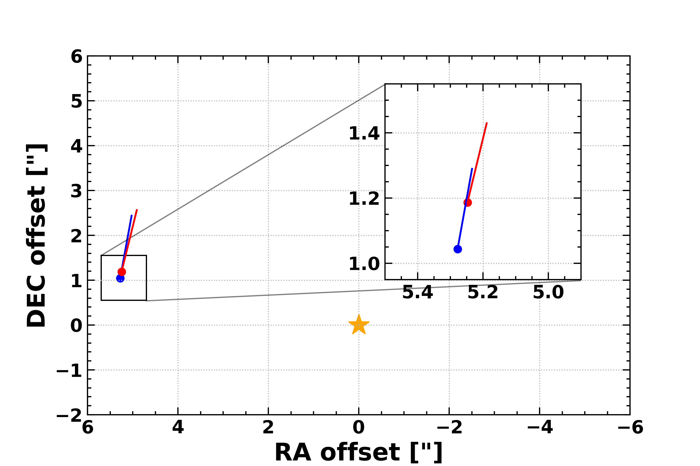
Figure 8: Gl 896. Position and velocity direction of Gl 896B relative to Gl 896A at the beginning (2014 Aug 22 (21:00 UTC), blue) and end (2016 May 23 (11:35 UTC); red) of the Gaia DR2 astrometric time series (Lindegren et al., 2018). Velocity direction was computed from the Heintz (1984) orbital elements. The velocity direction has changed over the time interval, indicating departure from the assumption of linear motion during the Gaia observations. Inset: closer view of position and velocity at beginning and end of Gaia time series, for clarity.

Figure 7 shows a selection of orbits from the posterior of the Gaia-only fit, as well as the WDS astrometric measurements (black circles) and Heintz (1984) orbit (red). Table 3 shows that the Heintz (1984) orbit is on the edge of the 68% minimum credible interval for our posterior distribution. Figure 8 shows the velocity direction at the beginning (2014 Aug 22 (21:00 UTC), blue) and end (2016 May 23 (11:35 UTC); red) of the Gaia DR2 time series (Lindegren et al., 2018), showing departure from the assumption of linear motion during Gaia DR2 observations. For this system, the Gaia-only fit did not outperform the time-series astrometric fit, as it had for DS Tuc AB.

Future Gaia data releases including plane-of-sky acceleration terms will improve the accuracy of orbital element constraint for this and other systems with non-linear motion during the Gaia astrometric observations.

4.2 Subsystems unresolved by Gaia, such as Kepler-444 BC

The method will not be accurate for systems where one or both objects are unresolved stellar binaries, as in the case of Kepler-444 BC (RUWE$=16.687$). Kepler-444 (a.k.a. BD+41 3306, HIP 94931, KOI-3158) consists of a spectroscopic binary, Kepler-444 BC (M_B = 0.29$\pm$0.03 M_⊙, M_C = 0.25$\pm$0.03 M_⊙ via mass-magnitude relation of Delfosse et al. 2000, as applied by Dupuy et al. 2016), at 1.8″separation from the primary Kepler-444 A (Carney 1983; M = 0.76$\pm$0.04 via asteroseismology). Kepler-444 A hosts five transiting sub-Earth radius planets (Campante et al., 2015). Kepler-444 BC has a high RUWE due to the unresolved binary, and we find that Gaia astrometry is not reliable for determining the orbit of BC relative to A.

Table 4: Comparison of the unsuccessful Kepler-444 Gaia LOFTI fit to Dupuy et al. 2016

Element	Dupuy et.al. 2016	Gaia Position/Velocity fit
		Mean	Std Dev	Mode	68.3% Min CI	95.4% Min CI
$a$ (AU)	36.7${}^{+0.7}_{-0.9}$	78.3	65.5	46.6	(42.7, 76.0)	(41.1, 171.2)
$P$ (yrs)	198${}^{+8}_{-9}$	740	1700	280	(250, 600)	(230, 2020)
$e$	0.864 $\pm$ 0.023	0.44	0.14	0.52	(0.31, 0.62)	(0.18, 0.67)
$i$ (°)	90.4${}^{+3.4}_{-3.6}$	133.4	11.1	138.9	(124.8, 148.5)	(112.3, 151.7)
$\omega$ (°)	342.8${}^{+3.2}_{-2.6}$	6	89	-80	(-90, 107)	(-150, 174)
$\Omega$ (°)	73.1 $\pm$ 0.9	77	45	121	(-57, 132)	(-13, 134)
$T_{0}$ (JD)	2488500 $\pm$ 900	2328900	376400	2393700	(2367900, 2402600)	(2126200, 2408900)
Periastron (AU)	5.0${}^{+0.9}_{-1.0}$	43	26	25	(16, 48)	(14, 100)

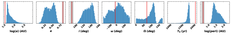
Figure 9: Unsuccessful fit: Kepler-444. The Gaia astrometry is not sufficient to accurately constrain the orbit of this system due to one component being a close binary unresolved by GaiaṖosterior distributions of orbital elements for the LOFTI fit of Kepler-444 are shown. The mean values reported in D16 are marked by red lines, error in grey. The LOFTI posteriors are not consistent with the established orbit for the system.

We performed an orbit fit anyway to demonstrate the effect of the unresolved binary on the orbit determination. Table 4 displays the results of our Gaia linear velocity fit as compared to the established orbit of Dupuy et al. (2016). For the majority of parameters the established value does not even fall within the 95% confidence interval for our posterior.

The accuracy of the Gaia orbit fitting technique will be impacted when wide binaries contain subsystems. The extent to which subsystems may bias Gaia measurements remains unknown, but is partially captured in the RUWE parameter. We therefore recommend careful consideration of the RUWE of components when applying this technique.

4.3 Possible source confusion due to small separations, such as RW Aurigae

RW Aurigae is a T-Tauri system with at least two components, RW Aurigae A and B, with a separation of $\rho=1.5$″(Duchêne et al., 1999). Rodriguez et al. (2018) imaged disks around both A and B with ALMA, with disk inclinations $i_{A}=57.68\degree\pm 0.86\degree$ and $i_{B}=72.08\degree\pm 7.98\degree$ in ALMA Band 7, and found evidence that the disks had been disrupted by a possible stellar flyby. The two components are resolved in Gaia DR2, making this an interesting case for studying the alignment between the stellar orbit and the disks.

The 1.5″ separation between the components is much closer than other systems we explored here. Table 1 shows that RW Aurigae B has a high RUWE value (A:RUWE = 1.774; B: RUWE = 28.904). The high RUWE for component B could be due to an unresolved companion, as with Kepler-444. However, Kraus et al. 2011 ruled out companions with contrasts down to $\Delta K^{\prime}\sim$ 3.5 mags at 40 mas, and $\Delta K^{\prime}\sim$ 1.5 mags down to 20 mas in non-redundant aperture masked (NRM) imaging. To induce sufficient noise that B would have RUWE $\sim$ 30, a companion around RW Aurigae B would likely be wide and bright enough to be detectable by NRM (Kraus et al. in prep).

We suggest that the binary separation might introduce confusion in the astrometric solution. The orientation of the two components relative to the scan direction could cause projection effects when projected to the line spread function (LSF) (Gaia Collaboration et al., 2016). If the components are oriented nearly perpendicular to the scan direction, their profiles might blend and overlap when projected to the 1-D LSF, and confuse the astrometric solution. Kraus et al. (in prep) have found that for binary systems of roughly equal brightness, those with projected separations below $\rho\sim$1.5″ show elevated RUWE values for both components, especially the secondary. This effect could be the source of the elevated RUWE values for RW Aurigae.

We attempted an orbit fit to the Gaia data. The large errors on astrometric parameters meant that orbital parameters were poorly constrained by the data, and did not produce reliable results. Improved astrometry is needed to apply LOFTI.

5 Discussion and Conclusion

We have shown that Gaia astrometry alone can be used to provide scientifically interesting constraints on orbital elements in several test cases. The suitability of Gaia astrometry for any particular binary system must be carefully assessed before being used as the sole observational constraint for stellar orbit fitting. Binaries for which both components have RUWE $\approx$1.0 are good candidates for this technique. Care should be taken in cases where the orbital period is short enough to influence the Gaia astrometric result, where there might be unresolved inner companions, or where a resolved yet close separation binary may influence the Gaia astrometry. Careful consideration of the RUWE value of both components must be undertaken before relying on orbit fitting results from Gaia measurements alone.

The lack of the requirement for long-term astrometric monitoring to constrain orbital elements enables new investigations on many topics in binary star science. Co-planarity between binary and planetary orbits, or binary orbit and protoplanetary disk, is easily determined, as in the case of DS Tuc, or ruled out, as with Kepler-25 and KOI-1803. The potential for the binary orbit to have influenced development of a disk or planetary system can be ruled out in systems with low eccentricity or wide periastron distances, as with GK/GI Tau.

While Gaia astrometry alone does not fully determine an orbit, we have already demonstrated how the ease of access and accuracy of Gaia measurements can readily contribute to study of binary system dynamics and star and planet formation.

Appendix A Equations for position, velocity, and acceleration given orbital elements

Here we present the equations we have used to compute predicted position, velocity, and acceleration for a trial orbit in our LOFTI orbit fits.

For fitting orbits to stellar binaries in Gaia, we reduce the two-body system to the relative motion of one mass-less point particle around a central object of mass equal to the total system mass. Taking the central body of a 2-body Keplerian orbit to be at the origin of the 3-d cartesian coordinate system, the position of the orbiting body is given by the coordinates (X,Y,Z), where +X is the reference direction, equal to +Declination in the on-sky coordinates. +Y is the +RA direction, and +Z is the line of sight direction towards the observer. This is the coordinate system presented in Murray & Correia (2010), from which we base our derivation. We note that this is different from the typical radial velocity convention that is often used elsewhere, in which -Z is toward the observer.

The orbital elements are: $a$ (semi-major axis) [and thus $P$ (period - derived from Kepler’s 3^rd law utilizing the total system mass and parallactic distance)], $t_{0}$ (time of periastron passage), $e$ (eccentricity), $i$ (inclination), $\omega$ (argument of periastron - angle from ascending node to periapse), and $\Omega$ (longitude of periastron - angle of location of ascending node from reference direction).

A.1 Positions

Murray & Correia (2010) Equations 53, 54, and 55 derive the following formulae for projecting orbital elements onto the plane of the sky:

$$X=r[\cos\Omega\cos(\omega+f)-\sin\Omega\sin(\omega+f)\cos i]$$ (A1)

$$Y=r[\sin\Omega\cos(\omega+f)-\cos\Omega\sin(\omega+f)\cos i]$$ (A2)

$$Z=r\sin(\omega+f)\sin i$$ (A3)

+X and +Y correspond to the observed +$\Delta$Dec ($\Delta\delta$) and +$\Delta$RA ($\Delta\alpha$) respectively between the orbiting body and central object. In this system +Z is defined toward the observer, contrary to the more commonly used radial velocity convention.

The radius of the orbiting body in the orbital plane is denoted as $r$, and is given by:

$$r=\frac{a(1-e^{2})}{1+e\cos f}$$ (A4)

The true anomaly is denoted as $f$, and is given by solving Kepler’s equation at the observation date (for Gaia DR2 this is 2015.5):

$$M=\frac{2\pi}{P}\big{(}t-t_{o}\big{)}$$ (A5)

$${\color[rgb]{0,0,0}M=E-e\sin E}$$ (A6)

which is a transcendental equation which must be solved numerically. In this case, $P$ is derived from Kepler’s 3rd law as $T=\sqrt{\frac{4\pi^{2}a^{3}}{\mu}}$, where $\mu=G(m_{1}+m_{2})$. The true anomaly then is given by:

$$f=2\,\arctan\left(\,\sqrt{\frac{1+e\,}{1-e\,}}\tan{\frac{E}{2}}\,\right)$$ (A7)

A.2 Velocities

Murray & Correia (2010) derive in Equation 63 the formula for velocity in the Z direction (radial velocity) as:

$$\dot{Z}=\dot{r}\sin(\omega+f)\sin i+r\dot{f}\cos(\omega+f)\sin i$$ (A8)

where $\dot{Z}$ is the time derivative of Z. In the equations above, only $r$, $\dot{r}$, and $f$ vary with time.

The time derivatives of X and Y give the velocity in the X and Y direction, which corresponds to proper motion in the Dec and RA directions respectively ($\mu_{\delta}$ and $\mu_{\alpha}$).

$$\begin{multlined}\dot{X}=\dot{r}\,\big{[}\,\cos\Omega\cos(\omega+f)-\sin\Omega\sin(\omega+f)\cos i\,\big{]}+\\ r\dot{f}\,\big{[}\,-\cos\Omega\sin(\omega+f)-\sin\Omega\cos(\omega+f)\cos i\,\big{]}\end{multlined}\dot{X}=\dot{r}\,\big{[}\,\cos\Omega\cos(\omega+f)-\sin\Omega\sin(\omega+f)\cos i\,\big{]}+\\ r\dot{f}\,\big{[}\,-\cos\Omega\sin(\omega+f)-\sin\Omega\cos(\omega+f)\cos i\,\big{]}$$ (A9)

$$\begin{multlined}\dot{Y}=\dot{r}\,\big{[}\sin\Omega\cos(\omega+f)+\cos\Omega\sin(\omega+f)\cos i\,\big{]}+\\ r\dot{f}\,\big{[}-\sin\Omega\sin(\omega+f)+\cos\Omega\cos(\omega+f)\cos i\,\big{]}\end{multlined}\dot{Y}=\dot{r}\,\big{[}\sin\Omega\cos(\omega+f)+\cos\Omega\sin(\omega+f)\cos i\,\big{]}+\\ r\dot{f}\,\big{[}-\sin\Omega\sin(\omega+f)+\cos\Omega\cos(\omega+f)\cos i\,\big{]}$$ (A10)

where $\dot{r}$ and $r\dot{f}$ are the time rate of change of separation and angular distance from the focus of the ellipse (the central body). Equations 31 and 32 in Murray & Correia (2010) define $\dot{r}$ and $r\dot{f}$ in terms of $a$ , $e$ , and $f$:

$$\dot{r}=\frac{na}{\sqrt{1-e^{2}}}e\sin f$$ (A11)

$$r\dot{f}=\frac{na}{\sqrt{1-e^{2}}}\big{(}1+e\cos f\big{)}$$ (A12)

where $n=\frac{2\pi}{T}$.

And the final position and velocity equations become:

$$\begin{multlined}X=\frac{a(1-e^{2})}{1+e\cos f}(\cos\Omega\cos(\omega+f)-\sin\Omega\sin(\omega+f)\cos i)=\Delta\delta\end{multlined}X=\frac{a(1-e^{2})}{1+e\cos f}(\cos\Omega\cos(\omega+f)-\sin\Omega\sin(\omega+f)\cos i)=\Delta\delta$$ (A13)

$$\begin{multlined}Y=\frac{a(1-e^{2})}{1+e\cos f}(\sin\Omega\cos(\omega+f)-\cos\Omega\sin(\omega+f)\cos i)=\Delta\alpha\end{multlined}Y=\frac{a(1-e^{2})}{1+e\cos f}(\sin\Omega\cos(\omega+f)-\cos\Omega\sin(\omega+f)\cos i)=\Delta\alpha$$ (A14)

$$Z=\frac{a(1-e^{2})}{1+e\cos f}\sin(\omega+f)\sin i$$ (A15)

$$\begin{multlined}\dot{X}=\frac{na}{\sqrt{1-e^{2}}}\;[\;e\sin f(\cos\Omega\cos(\omega+f)-\sin\Omega\sin(\omega+f)\cos i)\;+\\ \big{(}1+e\cos f\big{)}(-\cos\Omega\sin(\omega+f)-\sin\Omega\cos(\omega+f)\cos i)\;]=\mu_{\delta}\end{multlined}\dot{X}=\frac{na}{\sqrt{1-e^{2}}}\;[\;e\sin f(\cos\Omega\cos(\omega+f)-\sin\Omega\sin(\omega+f)\cos i)\;+\\ \big{(}1+e\cos f\big{)}(-\cos\Omega\sin(\omega+f)-\sin\Omega\cos(\omega+f)\cos i)\;]=\mu_{\delta}$$ (A16)

$$\begin{multlined}\dot{Y}=\frac{na}{\sqrt{1-e^{2}}}\;[\;e\sin f(\sin\Omega\cos(\omega+f)+\cos\Omega\sin(\omega+f)\cos i)\;+\\ \big{(}1+e\cos f\big{)}(-\sin\Omega\sin(\omega+f)+\cos\Omega\cos(\omega+f)\cos i)\;]=\mu_{\alpha}\end{multlined}\dot{Y}=\frac{na}{\sqrt{1-e^{2}}}\;[\;e\sin f(\sin\Omega\cos(\omega+f)+\cos\Omega\sin(\omega+f)\cos i)\;+\\ \big{(}1+e\cos f\big{)}(-\sin\Omega\sin(\omega+f)+\cos\Omega\cos(\omega+f)\cos i)\;]=\mu_{\alpha}$$ (A17)

$$\begin{multlined}\dot{Z}=\frac{na}{\sqrt{1-e^{2}}}\big{[}e\sin f\sin(\omega+f)\sin i+\big{(}1+e\cos f\big{)}\cos(\omega+f)\sin i\big{]}=v_{radial}\end{multlined}\dot{Z}=\frac{na}{\sqrt{1-e^{2}}}\big{[}e\sin f\sin(\omega+f)\sin i+\big{(}1+e\cos f\big{)}\cos(\omega+f)\sin i\big{]}=v_{radial}$$ (A18)

A.3 Accelerations

Future Gaia data releases will include terms for accelerations in the plane of sky. For completeness, we derive here equations for $\ddot{X}$, $\ddot{Y}$, $\ddot{Z}$ in terms of orbital elements, anticipating the use of these measurements in future orbit fitting with Gaia.

Beginning with Equations (A8)-(A10), we derive the second time derivative for X, Y, and Z position as

$$\begin{multlined}\ddot{X}=(\ddot{r}-r\dot{f}^{2})\,\big{[}\,\cos\Omega\cos(\omega+f)-\sin\Omega\sin(\omega+f)\,\cos i\,\big{]}\;+\\ (-2\dot{r}\dot{f}-r\ddot{f})\,\big{[}\,\cos\Omega\sin(\omega+f)+\sin\Omega\cos(\omega+f)\cos i\,\big{]}\end{multlined}\ddot{X}=(\ddot{r}-r\dot{f}^{2})\,\big{[}\,\cos\Omega\cos(\omega+f)-\sin\Omega\sin(\omega+f)\,\cos i\,\big{]}\;+\\ (-2\dot{r}\dot{f}-r\ddot{f})\,\big{[}\,\cos\Omega\sin(\omega+f)+\sin\Omega\cos(\omega+f)\cos i\,\big{]}$$ (A19)

$$\begin{multlined}\ddot{Y}=(\ddot{r}-r\dot{f}^{2})\,\big{[}\,\sin\Omega\cos(\omega+f)+\cos\Omega\sin(\omega+f)\cos i\,\big{]}\;+\\ (2\dot{r}\dot{f}+r\ddot{f})\,\big{[}\,\sin\Omega\sin(\omega+f)+\cos\Omega\cos(\omega+f)\cos i\,\big{]}\end{multlined}\ddot{Y}=(\ddot{r}-r\dot{f}^{2})\,\big{[}\,\sin\Omega\cos(\omega+f)+\cos\Omega\sin(\omega+f)\cos i\,\big{]}\;+\\ (2\dot{r}\dot{f}+r\ddot{f})\,\big{[}\,\sin\Omega\sin(\omega+f)+\cos\Omega\cos(\omega+f)\cos i\,\big{]}$$ (A20)

$$\begin{multlined}\ddot{Z}=\sin{i}\,\big{[}\,(\ddot{r}-r\dot{f}^{2}\,)\,\sin{(\omega+f)}+(2\dot{r}\dot{f}+r\ddot{f})\,\cos(\omega+f)\,\big{]}\end{multlined}\ddot{Z}=\sin{i}\,\big{[}\,(\ddot{r}-r\dot{f}^{2}\,)\,\sin{(\omega+f)}+(2\dot{r}\dot{f}+r\ddot{f})\,\cos(\omega+f)\,\big{]}$$ (A21)

Klioner (2016) gives two expressions for $\dot{E}$:

$$\dot{E}=\frac{n}{1-e\cos E}$$ (A22)

$$\dot{E}=\frac{an}{r}=\frac{n\;(1+e\cos{f})}{1-e^{2}}$$ (A23)

Thus we derive from Equation (A22):

$$\ddot{E}=\frac{-\;n\;e\;\sin{E}}{(1-e\cos{E})^{2}}\;\dot{E}=\frac{n^{2}\;e}{(1-e\cos{E})^{2}}\;\frac{\sin f}{\sqrt{1-e^{2}}}$$ (A24)

Or from (A23):

$$\ddot{E}=\frac{-n\;e\;\sin{f}}{1-e^{2}}\;\dot{f}$$ (A25)

From Equation (A12), we find that

$$\dot{f}=\frac{n\sqrt{1-e^{2}}}{(1-e\cos E)^{2}}=\dot{E}\frac{\sqrt{1-e^{2}}}{1-e\cos E}=\dot{E}\;\frac{\sin f}{\sin E}$$ (A26)

Where $\sin f=\frac{\sqrt{1-e^{2}}\sin E}{1-e\cos E}$.

Rewriting (A11) as:

$$\dot{r}=a\;e\;\dot{E}\;\sin{E}\;$$ (A27)

so

$$\ddot{r}=a\,e\,\cos{E}\,\dot{E}^{2}\;+\;a\,e\,\sin{E}\;\ddot{E}$$ (A28)

And from Equation (A26) we derive:

$$\ddot{f}=\ddot{E}\;\frac{\sqrt{1-e^{2}}}{1-e\cos E}+\dot{E}^{2}\,\frac{e\sqrt{1-e^{2}}\sin E}{(1-e\cos E)^{2}}$$ (A29)

Which reduces to:

$$\ddot{f}=\ddot{E}\;\frac{\sin f}{\sin E}+\dot{E}^{2}\,\frac{e\sin{f}}{1-e\cos E}$$ (A30)

This allows the calculation of all needed variables for computing $\ddot{X}$, $\ddot{Y}$, and $\ddot{Z}$.

Appendix B The LOFTI python tool

Documentation, tutorials, and illustration of functions are provided at the lofti_gaiaDR2 GitHub repository. Readers are directed to that repository for a more in-depth discussion of functionality.

Briefly, the lofti_gaiaDR2 python tool wraps the functionality of the LOFTI method described in Section 2.1 into a minimal python user interface. The user inputs the Gaia DR2 source id numbers, which can be found at the Gaia archive, the mass and uncertainties for each component, and a minimum number of desired orbits, into the fitorbit module. fitorbit queries the Gaia repository for the observational constraints, and runs trial orbits for the second source relative to the first source until the minimum desired number of orbits are accepted.

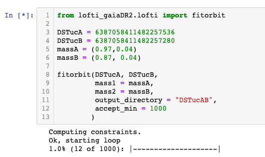
Figure 10: Example usage of lofti.fitorbit to use Gaia archive measurements to fit the orbit of DS Tuc B relative to DS Tuc A. The user inputs the two Gaia source ids, masses and uncertainties, an output directory to store the accepted orbits, and an minimum number of accepted orbits desired. The minimum orbits desired was set to 1000 for this demonstration, however to obtain a statistically meaningful result that samples the multi-dimensional posterior well, a minimum of $\geq$10⁵ orbits is recommended. The function queries the Gaia archive to obtain the measurement constraints, and runs trial orbits, updating the user via the progress bar, until the minimum number of orbits is accepted.

Figure 10 shows example input and output for fitorbit using the Gaia source ids for DS Tuc A and B given in Table 1, and masses from Newton et al. 2019. The source ids, masses, directory for storing results, and minimum desired orbits are input to fitorbit. If masses are omitted, the function will prompt the user to supply them. fitorbit runs trial orbits using the priors and acceptance criteria given in Section 2.1, writes accepted orbital parameters to a file contained in the specified output directory, and reports progress towards desired orbits through the progress bar. The function will provide a warning if either object has RUWE $\geq$ 1.2. If the Gaia archive includes radial velocity measurements for both objects, it will be automatically incorporated into the fit. At this time, no other user inputs, such as time-series astrometry or independently determined radial velocities, are accepted. The function fits using Gaia measurements alone.

lofti_gaiaDR2 includes the plotting function makeplots. The makeplots function produces plots of the fitorbit output like the ones included in this paper. Specifically, calling makeplots for the output file from fitorbit will produce sky plots like Figure 2, distributions of computed positions ($X,Y,Z$), velocities ($\dot{X},\dot{Y},\dot{Z}$), and accelerations ($\ddot{X},\ddot{Y},\ddot{Z}$) of the posterior orbits, a 3-dimensional orbit plot of selected orbits, 1-dimensional posterior distributions of orbital parameters like Figure 3, and a statistics file describing the distributions of orbital parameters. Each of these outputs can be toggled on and off through keywords in the function call. Users can choose to limit $\Omega$ or $\omega$ to [0,180] deg interval if no RV measurements were used, plot semi-major axis or periastron in log scale, or truncate the long tail of the semi-major axis distribution through function keywords. The outputs are written to the user specified directory.

Python packages numpy, matplotlib, astropy, astroquery, and pickle are dependencies for the lofti_gaiaDR2 python tool. lofti_gaiaDR2 can be installed via pip by calling pip install lofti_gaiaDR2 or through the the lofti_gaia github repository.

References

- Aitken (1918) Aitken, R. G. 1918, The binary stars
- Akeson & Jensen (2014) Akeson, R. L., & Jensen, E. L. N. 2014, ApJ, 784, 62
- Akeson et al. (2019) Akeson, R. L., Jensen, E. L. N., Carpenter, J., et al. 2019, ApJ, 872, 158
- Artymowicz (1992) Artymowicz, P. 1992, PASP, 104, 769
- Artymowicz & Lubow (1994) Artymowicz, P., & Lubow, S. H. 1994, ApJ, 421, 651
- Bate (2000) Bate, M. R. 2000, MNRAS, 314, 33
- Bate et al. (2002) Bate, M. R., Bonnell, I. A., & Bromm, V. 2002, MNRAS, 336, 705
- Batygin (2012) Batygin, K. 2012, Nature, 491, 418
- Benedict et al. (2016) Benedict, G. F., Henry, T. J., Franz, O. G., et al. 2016, AJ, 152, 141
- Blunt et al. (2017) Blunt, S., Nielsen, E. L., De Rosa, R. J., et al. 2017, AJ, 153, 229
- Blunt et al. (2019) Blunt, S., Wang, J., Angelo, I., et al. 2019, arXiv e-prints, arXiv:1910.01756
- Boss & Bodenheimer (1979) Boss, A. P., & Bodenheimer, P. 1979, ApJ, 234, 289
- Bower et al. (2011) Bower, G. C., Bolatto, A., Ford, E. B., et al. 2011, ApJ, 740, 32
- Bryan et al. (2020) Bryan, M. L., Chiang, E., Bowler, B. P., et al. 2020, arXiv e-prints, arXiv:2002.11131
- Burkert & Bodenheimer (1993) Burkert, A., & Bodenheimer, P. 1993, MNRAS, 264, 798
- Campante et al. (2015) Campante, T. L., Barclay, T., Swift, J. J., et al. 2015, ApJ, 799, 170
- Carney (1983) Carney, B. W. 1983, AJ, 88, 623
- Chatterjee et al. (2008) Chatterjee, S., Ford, E. B., Matsumura, S., & Rasio, F. A. 2008, ApJ, 686, 580
- Christy & Harrington (1978) Christy, J. W., & Harrington, R. S. 1978, AJ, 83, 1005
- Czekala et al. (2019) Czekala, I., Chiang, E., Andrews, S. M., et al. 2019, ApJ, 883, 22
- Deacon et al. (2016) Deacon, N. R., Kraus, A. L., Mann, A. W., et al. 2016, MNRAS, 455, 4212
- Delfosse et al. (2000) Delfosse, X., Forveille, T., Ségransan, D., et al. 2000, A&A, 364, 217
- Duchêne & Kraus (2013) Duchêne, G., & Kraus, A. 2013, ARA&A, 51, 269
- Duchêne et al. (1999) Duchêne, G., Monin, J. L., Bouvier, J., & Ménard, F. 1999, A&A, 351, 954
- Dupuy et al. (2016) Dupuy, T. J., Kratter, K. M., Kraus, A. L., et al. 2016, ApJ, 817, 80
- Duquennoy & Mayor (1991) Duquennoy, A., & Mayor, M. 1991, A&A, 500, 337
- Fabrycky & Tremaine (2007) Fabrycky, D., & Tremaine, S. 2007, ApJ, 669, 1298
- Fulton & Petigura (2018) Fulton, B. J., & Petigura, E. A. 2018, AJ, 156, 264
- Gaia Collaboration et al. (2018) Gaia Collaboration, Brown, A. G. A., Vallenari, A., et al. 2018, A&A, 616, A1
- Gaia Collaboration et al. (2016) Gaia Collaboration, G., Prusti, T., de Bruijne, J. H. J., et al. 2016, Astronomy & Astrophysics, Volume 595, id.A1, 36 pp., 595, doi:10.1051/0004-6361/201629272. http://arxiv.org/abs/1609.04153http://dx.doi.org/10.1051/0004-6361/201629272
- Godoy-Rivera & Chanamé (2018) Godoy-Rivera, D., & Chanamé, J. 2018, MNRAS, 479, 4440
- Goldreich & Tremaine (1980) Goldreich, P., & Tremaine, S. 1980, ApJ, 241, 425
- Hale (1994) Hale, A. 1994, AJ, 107, 306
- Hartigan et al. (1994) Hartigan, P., Strom, K. M., & Strom, S. E. 1994, ApJ, 427, 961
- Heintz (1978) Heintz, W. D. 1978, Double stars, Vol. 15
- Heintz (1984) —. 1984, AJ, 89, 1063
- Herczeg & Hillenbrand (2014) Herczeg, G. J., & Hillenbrand, L. A. 2014, ApJ, 786, 97
- Hunter (2007) Hunter, J. D. 2007, Computing In Science & Engineering, 9, 90
- Jensen et al. (2004) Jensen, E. L. N., Mathieu, R. D., Donar, A. X., & Dullighan, A. 2004, ApJ, 600, 789
- Kenyon & Hartmann (1995) Kenyon, S. J., & Hartmann, L. 1995, ApJS, 101, 117
- Kiselev & Kiyaeva (1980) Kiselev, A. A., & Kiyaeva, O. V. 1980, AZh, 57, 1227
- Kiyaeva et al. (2017) Kiyaeva, O. V., Romanenko, L. G., & Zhuchkov, R. Y. 2017, Astronomy Letters, 43, 316
- Klioner (2016) Klioner, S. A. 2016, arXiv e-prints, arXiv:1609.00915
- Kozai (1962) Kozai, Y. 1962, AJ, 67, 591
- Kraus & Hillenbrand (2009) Kraus, A. L., & Hillenbrand, L. A. 2009, ApJ, 703, 1511
- Kraus et al. (2012) Kraus, A. L., Ireland, M. J., Hillenbrand, L. A., & Martinache, F. 2012, ApJ, 745, 19
- Kraus et al. (2016) Kraus, A. L., Ireland, M. J., Huber, D., Mann, A. W., & Dupuy, T. J. 2016, AJ, 152, 8
- Kraus et al. (2011) Kraus, A. L., Ireland, M. J., Martinache, F., & Hillenbrand, L. A. 2011, ApJ, 731, 8
- Kraus et al. (2008) Kraus, A. L., Ireland, M. J., Martinache, F., & Lloyd, J. P. 2008, \Apj, 679, 762
- Lai (2014) Lai, D. 2014, MNRAS, 440, 3532
- Lee et al. (2019) Lee, A. T., Offner, S. S. R., Kratter, K. M., Smullen, R. A., & Li, P. S. 2019, arXiv e-prints, arXiv:1911.07863
- Lidov (1962) Lidov, M. L. 1962, Planet. Space Sci., 9, 719
- Lindegren (2018) Lindegren, L. 2018, gAIA-C3-TN-LU-LL-124. http://www.rssd.esa.int/doc_fetch.php?id=3757412
- Lindegren et al. (2018) Lindegren, L., Hernández, J., Bombrun, A., et al. 2018, A&A, 616, A2
- Lissauer et al. (2011) Lissauer, J. J., Ragozzine, D., Fabrycky, D. C., et al. 2011, ApJS, 197, 8
- Lissauer et al. (2014) Lissauer, J. J., Marcy, G. W., Bryson, S. T., et al. 2014, ApJ, 784, 44
- Long et al. (2019) Long, F., Herczeg, G. J., Harsono, D., et al. 2019, ApJ, 882, 49
- Mann et al. (2019) Mann, A. W., Dupuy, T., Kraus, A. L., et al. 2019, ApJ, 871, 63
- Marcy et al. (2014) Marcy, G. W., Isaacson, H., Howard, A. W., et al. 2014, ApJS, 210, 20
- Mason et al. (2001) Mason, B. D., Wycoff, G. L., Hartkopf, W. I., Douglass, G. G., & Worley, C. E. 2001, AJ, 122, 3466
- Mills et al. (2019) Mills, S. M., Howard, A. W., Weiss, L. M., et al. 2019, AJ, 157, 145
- Moe & Di Stefano (2017) Moe, M., & Di Stefano, R. 2017, ApJS, 230, 15
- Murray & Correia (2010) Murray, C. D., & Correia, A. C. M. 2010, Keplerian Orbits and Dynamics of Exoplanets, ed. S. Seager, 15–23
- Newton et al. (2019) Newton, E. R., Mann, A. W., Tofflemire, B. M., et al. 2019, arXiv e-prints, arXiv:1906.10703
- Offner et al. (2016) Offner, S. S. R., Dunham, M. M., Lee, K. I., Arce, H. G., & Fielding, D. B. 2016, ApJ, 827, L11
- Offner et al. (2010) Offner, S. S. R., Kratter, K. M., Matzner, C. D., Krumholz, M. R., & Klein, R. I. 2010, ApJ, 725, 1485
- Oliphant (2006) Oliphant, T. E. 2006, A guide to NumPy, Vol. 1 (Trelgol Publishing USA)
- Papaloizou & Terquem (1995) Papaloizou, J. C. B., & Terquem, C. 1995, MNRAS, 274, 987
- Pearce et al. (2019) Pearce, L. A., Kraus, A. L., Dupuy, T. J., et al. 2019, AJ, 157, 71
- Plavchan et al. (2013) Plavchan, P., Güth, T., Laohakunakorn, N., & Parks, J. R. 2013, A&A, 554, A110
- Price-Whelan et al. (2018) Price-Whelan, A. M., Sip’ocz, B. M., G”unther, H. M., et al. 2018, aj, 156, 123
- Raghavan et al. (2010) Raghavan, D., McAlister, H. A., Henry, T. J., et al. 2010, ApJS, 190, 1
- Rasio & Ford (1996) Rasio, F. A., & Ford, E. B. 1996, Science, 274, 954
- Rizzuto et al. (2018) Rizzuto, A. C., Vanderburg, A., Mann, A. W., et al. 2018, AJ, 156, 195
- Rodriguez et al. (2018) Rodriguez, J. E., Loomis, R., Cabrit, S., et al. 2018, ApJ, 859, 150
- Rowe et al. (2014) Rowe, J. F., Bryson, S. T., Marcy, G. W., et al. 2014, ApJ, 784, 45
- Rubin & Ford (1970) Rubin, V. C., & Ford, W. Kent, J. 1970, ApJ, 159, 379
- Schaefer et al. (2014) Schaefer, G. H., Prato, L., Simon, M., & Patience, J. 2014, AJ, 147, 157
- Ségransan et al. (2000) Ségransan, D., Delfosse, X., Forveille, T., et al. 2000, A&A, 364, 665
- Shu et al. (1987) Shu, F. H., Adams, F. C., & Lizano, S. 1987, ARA&A, 25, 23
- Silva Aguirre et al. (2015) Silva Aguirre, V., Davies, G. R., Basu, S., et al. 2015, MNRAS, 452, 2127
- Simon et al. (2017) Simon, M., Guilloteau, S., Di Folco, E., et al. 2017, ApJ, 844, 158
- Skrutskie et al. (2006) Skrutskie, M. F., Cutri, R. M., Stiening, R., et al. 2006, AJ, 131, 1163
- Stapelfeldt et al. (1998) Stapelfeldt, K. R., Krist, J. E., Ménard, F., et al. 1998, ApJ, 502, L65
- Steffen et al. (2012) Steffen, J. H., Fabrycky, D. C., Ford, E. B., et al. 2012, MNRAS, 421, 2342
- Thompson et al. (2018) Thompson, S. E., Coughlin, J. L., Hoffman, K., et al. 2018, ApJS, 235, 38
- Tobin et al. (2016) Tobin, J. J., Kratter, K. M., Persson, M. V., et al. 2016, Nature, 538, 483
- Tokovinin (2018a) Tokovinin, A. 2018a, AJ, 155, 160
- Tokovinin (2018b) —. 2018b, ApJS, 235, 6
- Tokovinin & Latham (2017) Tokovinin, A., & Latham, D. W. 2017, ApJ, 838, 54
- Tokovinin & Moe (2019) Tokovinin, A., & Moe, M. 2019, MNRAS, 2954
- Torres et al. (2006) Torres, C. A. O., Quast, G. R., da Silva, L., et al. 2006, A&A, 460, 695
- Torres (1988) Torres, G. 1988, Ap&SS, 147, 257
- Weidenschilling & Marzari (1996) Weidenschilling, S. J., & Marzari, F. 1996, Nature, 384, 619
- Winn et al. (2004) Winn, J. N., Holman, M. J., Johnson, J. A., Stanek, K. Z., & Garnavich, P. M. 2004, ApJ, 603, L45
- Wirtanen (1941) Wirtanen, C. A. 1941, PASP, 53, 340
- Ziegler et al. (2019) Ziegler, C., Tokovinin, A., Briceno, C., et al. 2019, arXiv e-prints, arXiv:1908.10871