Coupled criticality analysis of inflation and unemployment

Abstract

In this paper, we are interested to focus on the critical periods in economy which are characterized by large fluctuations in macroeconomic indicators. To capture unusual and large fluctuations of inflation and unemployment, we concentrate on the non-Gaussianity of their distributions. To this aim, by using the coupled multifractal approach, we analyze US data for a period of 70 years from 1948 until 2018 and measure the non-Gausianity of the distributions.Then, we investigate how the non-Gaussianity of the variables affect the coupling structure of them.

By applying the multifractal method, one can see that the non-Gaussianity depends on the scales. While the non-Gaussianity of unemployment is noticeable only for periods smaller than 1 year and for longer periods tends to Gaussian behavior, the non-Gaussianities of inflation persist for all time scales. Also, it is observed that the coupling structure of these variables tends to a Gaussian behavior after $2$ years.

Keywords: Non-Gaussianity, Bi-MRW, Inflation, Unemployment, Multifractality, Phillips curve

I Introduction

Unemployment and inflation are two important economic indices; their relation is meaningful for policy makers. Historically, there have been hot debates over the relation between unemployment and inflation, - starting with the observation of Phillips phillips .

Later, the huge debate was ignited about the strength and causal effect of the relation solow ; friedman ; phelps . The matter has been important because of its influence on government policies during the times of recession, but at other times as well taylor ; mishkin . Discussion over the matter is still a serious controversial issue in economics, see for example akerlof ; gali ; mankiw .

Yet, few works have considered the theoretical complexity of these variables, thus leading to the research questions of this paper safdari .

Of course, economics complexity has attracted a big deal of attention in recent years arthur ; deligatti ; Namaki1 ; farmer ; Hosseiny ; namaki ; helbing2013rethinking .

Economy can be considered as a big network of heterogenous agents which interact with each other and with their environment Schweitzer ; d2016complex ; chakrabarti ; Namaki2 ; Dragulescu ; Vandewalle ; hosseinyrole ; Aoyama2010 ; VRAC015complex ; hosseinygeommetry . It is reasonable to expect that inflation and unemployment as outcomes of these complex systems inherit complexity considerations.

This suggests a thorough analysis of these variables along advanced techniques available in complexity theory approach and applications Anderson99 ; Ivanova2002 ; Ausloos12 .

Looking at unemployment and inflation indices as simple variables may ignore some rich knowledge about their complexity. It has been shown for example that economic indicators and their coupling have nice scaling features Vandewalle98 ; Vandewalle1998 ; safdari . In fact, many economic variables present some multifractal nature Ivanova99 ; Grech ; Zhou . Such an observation suggests that inflation and unemployment data sets might exhibit non-Gaussian probability density function (PDF). This behavior may originate from the occurrence of large fluctuations in the system at extreme values.

In order to model the non-Gaussianity of some signal, a multifractal random walk (MRW) model has already been implemented; MRW is composed of the product of two processes with normal and log-normal PDFs Bacry01 ; Zahra . The variance of the log-normal part determines the strength of non-Gaussianity of the original signal Chabaud ; Ghas96 ; Ausloos2002 .

In order to go further, i.e. to capture the non-Gaussianity in the coupling of variables, we apply the bivariate Multifractal Random Walk (Bi-MRW) technique Muzy01 ; Muzy02 . Therefore, this approach leads us to obtain and to analyze the type of cross-correlations between large fluctuations in inflation and unemployment measures. Whence, the paper is organized as follows. In section 2, we explain the MRW and Bi-MRW methods; in section 3 and section 4, we present our findings and conclusions respectively.

II Methods

II.1 Multifractal Random Walk (MRW)

The Multifractal Random Walk (MRW) for analysing time series stems from turbulent cascade models Chabaud . These processes are useful for presenting the non-Gaussian behavior of time series.

The temporal fluctuations increment of a process at scale $s$ , $\delta_{s}x(t)=x(t+s)-x(t)$, can be modeled by the product of a normal and a log-normal process:

$$\delta_{s}x(t)=\epsilon_{s}(t)e^{\omega_{s}(t)},$$ (1)

where $\epsilon_{s}(t)$ and $\omega_{s}(t)$ are normal processes with zero mean and standard deviations equal to $\sigma(s)$ and $\lambda(s)$ respectively.

Based on Eq.(1), we can write a probability density function for $\delta_{s}x(t)$ as:

$$P_{s}(\delta_{s}x)=\int_{0}^{\infty}G_{s}(\ln\sigma(s))\frac{1}{\sigma(s)}F_{s}\left(\frac{\delta_{s}x}{\sigma(s)}\right)d(\ln\sigma(s)),$$ (2)

where

$$G_{s}(\ln\sigma(s)) = \frac{1}{\sqrt{2\pi}\lambda(s)}\exp\left[-\frac{(\ln\sigma(s)+\lambda^{2}(s))^{2}}{2\lambda^{2}(s)}\right],$$ (3)

and

$$F_{s}\left(\frac{\delta_{s}x}{\sigma(s)}\right) = \frac{1}{\sqrt{2\pi}}\exp\left[-\frac{\delta_{s}x^{2}}{2\sigma^{2}(s)}\right].$$ (4)

since $\lambda^{2}(s)$ is the variance of the log-normal part of the process. This parameter is the representative measure of the non-Gaussianity of the process; if $\lambda^{2}(s)\rightarrow 0$, the PDF of $\delta_{s}x(t)$ converges to a Gaussian distribution. An estimation of $\lambda^{2}(s)$ versus a scale $s$ is our way for presenting the effect of large fluctuations over different scales. Furthermore, for showing the effects of the rare events (in the PDF tails), high order moments of fluctuations of order $q$, denoted by $m_{q}$, can be calculated

$$m_{q}(\delta_{s}x)=\langle|(\delta_{s}x)|^{q}\rangle=\left[\int|\delta_{s}x|^{q}P_{s}(\delta_{s}x)d(\delta_{s}x)\right]^{\frac{1}{q}}.$$ (5)

A large value of $m_{q}$ implies a significant role of rare events. If this is found to be independent of $q$, the process is called monofractal; otherwise, it is called a multifractal Shayeganfar .

II.2 Joint Multifractal Approach: the Bi-MRW method

Muzy et al. Muzy01 ; Muzy02 have proposed the bivariate Multifractal Random Walk (Bi-MRW) method for analyzing two non-Gaussian stochastic processes (${\bf x}(t)=\{x_{1}(t),x_{2}(t)\}$) simultaneously, when the increments of each time series are supposed to be generated by the product of normal and log-normal processes:

$$\delta_{s}\textbf{x}(t)=\left(\delta_{s}x_{1}(t),\delta_{s}x_{2}(t)\right)=\left(\epsilon_{1}^{(s)}(t)e^{\omega_{1}^{(s)}(t)},\epsilon_{2}^{(s)}(t)e^{\omega_{2}^{(s)}(t)}\right),$$ (6)

in which $(\epsilon_{1}^{(s)},\epsilon_{2}^{(s)})$ and $(\omega_{1}^{(s)},\omega_{2}^{(s)})$ have joint normal PDF with zero mean.

Muzy et al., generalizing the MRW approach, consider the cross-correlation of stochastic variances of two processes Muzy01 . Practically, $(\epsilon_{1}^{(s)},\epsilon_{2}^{(s)})$ have a covariance matrix

$$\mathbf{\Sigma}_{(s)}\equiv\left(\begin{array}[]{cc}\sigma_{1}^{2}(s)&\Sigma(s)\\ \Sigma_{(}s)&\sigma_{2}^{2}(s)\\ \end{array}\right)$$ (7)

where $\Sigma(s)=\rho_{\epsilon}(s)\sigma_{1}(s)\sigma_{2}(s)$ Muzy01 .

The covariance matrix of $(\omega_{1}^{(s)},\omega_{2}^{(s)})$ is denoted by $\mathbf{\Lambda}_{(s)}$ and called a multifractal matrix Muzy01 ; it is given by

$$\mathbf{\Lambda}_{(s)}\equiv\left(\begin{array}[]{cc}\lambda_{1}^{2}(s)&\Lambda(s)\\ \Lambda(s)&\lambda_{2}^{2}(s)\\ \end{array}\right),$$ (8)

where $\Lambda(s)=\rho_{\omega}(s)\lambda_{1}(s)\lambda_{2}(s)$ and $\rho_{\omega}(s)$ is the multifractal correlation coefficient. The PDFs of $(\epsilon_{1}^{(s)}\;,\epsilon_{2}^{(s)})$, and $(\omega_{1}^{(s)}\;,\omega_{2}^{(s)})$ have the following form:

$$F_{s}(\epsilon_{1}^{(s)},\epsilon_{2}^{(s)}) = \frac{1}{2\pi\sqrt{{\rm Det}(\mathbf{\Sigma}_{(s)})}}\ \exp\left({-\frac{\epsilon_{(s)}^{\rm T}\cdot\mathbf{\Sigma}_{(s)}^{-1}\cdot\epsilon_{(s)}}{2}}\right)$$

$$G_{s}(\omega_{1}^{(s)},\omega_{2}^{(s)}) = \frac{1}{2\pi\sqrt{{\rm Det}(\mathbf{\Lambda}_{(s)})}}\ \exp\left({-\frac{\mathbf{\omega}^{\rm T}_{(s)}\cdot\mathbf{\Lambda}^{-1}_{(s)}\cdot\mathbf{\omega}_{(s)}}{2}}\right)\;.$$

Therefore, the joint PDF of the fluctuations increment vector $(\delta_{s}x_{1},\delta_{s}x_{2})$ is given by

$$P_{s}(\delta_{s}x_{1},\delta_{s}x_{2})=\int d(\ln\sigma_{1}(s))\int d(\ln\sigma_{2}(s))G_{s}\left(\ln\sigma_{1}(s),\ln\sigma_{2}(s)\right)\frac{1}{\sigma_{1}(s)}\frac{1}{\sigma_{2}(s)}F\left(\frac{\delta_{s}x_{1}}{\sigma_{1}(s)},\frac{\delta_{s}x_{2}}{\sigma_{2}(s)}\right)\;.$$ (11)

It follows from the above definitions of $G_{s}(\ln\sigma_{1}(s),\ln\sigma_{2}(s))$ and $F_{s}\left(\frac{\delta_{s}x_{1}}{\sigma_{1}(s)},\frac{\delta_{s}x_{2}}{\sigma_{2}(s)}\right)$ that

$$G_{s}\left(\ln\sigma_{1}(s),\ln\sigma_{2}(s)\right)=\frac{1}{2\pi\sqrt{\lambda^{2}_{1}(s)\lambda^{2}_{2}(s)-\Lambda^{2}(s)}}$$

$$\exp\left[-\frac{\lambda_{2}^{2}(s)\left[\ln\sigma_{1}(s)+\lambda_{1}^{2}(s)\right]^{2}+\lambda_{1}^{2}(s)\left[\ln\sigma_{2}(s)+\lambda_{2}^{2}(s)\right]^{2}-2\Lambda(s)\left[\ln\sigma_{1}(s)+\lambda_{1}^{2}(s)\right]\left[\ln\sigma_{2}(s)+\lambda_{2}^{2}(s)\right]}{2\left(\lambda^{2}_{1}(s)\lambda^{2}_{2}(s)-\Lambda^{2}(s)\right)}\right]$$

and

$$F_{s}\left(\frac{\delta_{s}x_{1}}{\sigma_{1}(s)},\frac{\delta_{s}x_{2}}{\sigma_{2}(s)}\right)=\frac{1}{2\pi\sqrt{\sigma^{2}_{1}(s)\sigma^{2}_{2}(s)-\Sigma^{2}(s)}}\exp\left[-\frac{\left[\sigma_{2}(s)\delta_{s}x_{1}\right]^{2}+\left[\sigma_{1}(s)\delta_{s}x_{2}\right]^{2}-2\Sigma(s)\delta_{s}x_{1}\delta_{s}x_{2}}{2\left(\sigma^{2}_{1}(s)\sigma^{2}_{2}(s)-\Sigma^{2}(s)\right)}\right].$$

It can be observed that $P_{s}(\delta_{s}x_{1},\delta_{s}x_{2})$ becomes equal to $P_{s}(\delta_{s}x_{1})P_{s}(\delta_{s}x_{2})$ when $\Lambda(s)$ and $\Sigma(s)$ tend to zero.

The $q$-th order moment of fluctuations increments for such two processes at scale $s$ can be written as

$$m^{joint}_{q}(\delta_{s}x_{1},\delta_{s}x_{2})=\langle|(\delta_{s}x_{1})|^{q}|(\delta_{s}x_{2})|^{q}\rangle=\left[\int\int|\delta_{s}x_{1}|^{q}|\delta_{s}x_{2}|^{q}P_{s}(\delta_{s}x_{1},\delta_{s}x_{2})d(\delta_{s}x_{1})d(\delta_{s}x_{2})\right]^{\frac{1}{q}}.$$ (14)

III Results

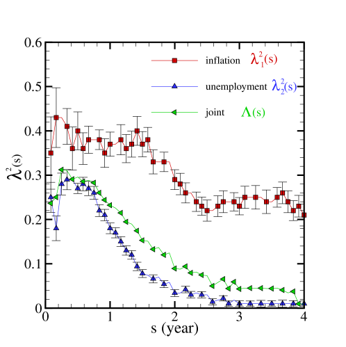
Figure 1: $\lambda^{2}(s)$ as a measure of non-Gaussianity for either unemployment ”($\triangle$)” or inflation ”$\Box$” and the value of the multifractal coefficient $\Lambda(s)$ over different time scales ”$s$”.

Thereafter, we can analyze both inflation and unemployment rates, provided by the U.S. Inflation Calculator inflation and U.S. Bureau of Labor Statistics USBLBunemployment , respectively. The data has been recorded monthly from January $1948$ until October $2018$. The non-Gaussian parameter $\lambda^{2}(s)$ and the joint multifractal coefficient $\Lambda(s)$ at scale $s$ are obtained from the integral form of cascading rules in Eqs. (2) and (11). The best values for $\lambda^{2}(s)$ and $\Lambda(s)$ at scale $s$, are for the global minimum of the chi-square, $\chi^{2}$ Agostini003 ; Sivia006 :

$$\chi^{2}(\Lambda(s);\Sigma(s))=\sum_{\delta_{s}{\bf x}}\frac{\left[P_{\rm data}(\delta_{s}{\bf x})-P_{\rm theory}(\delta_{s}{\bf x};\Lambda(s),\Sigma(s))\right]^{2}}{\sigma^{2}_{\rm data}(\delta_{s}{\bf x})+\sigma^{2}_{\rm theory}(\delta_{s}{\bf x};\Lambda(s),\Sigma(s))},$$ (15)

where $P_{\rm data}(\delta_{s}{\bf x})$ is the joint PDF computed from data, while $P_{\rm theory}(\delta_{s}{\bf x};\Lambda(s),\Sigma(s))$ is the theoretical joint PDF proposed in Eq.(11). By definition, $\sigma^{2}_{\rm data}(\delta_{s}{\bf x})$ and $\sigma^{2}_{\rm theory}(\delta_{s}{\bf x};\Lambda(s),\Sigma(s))$ are the mean standard deviation of $P_{\rm data}(\delta_{s}{\bf x})$ and $P_{\rm theory}(\delta_{s}{\bf x};\Lambda(s),\Sigma(s))$, respectively.

The best value of $\Lambda(s)$ for the theoretical joint PDF is obtained from the fit of the joint PDF to the data:

$$\chi^{2}(\Lambda(s)) = \sum_{\delta_{s}{\bf x}}\int d\Sigma(s)\left(\frac{\left[P_{\rm data}(\delta_{s}{\bf x},s)-P_{\rm theory}(\delta_{s}{\bf x};\Lambda(s),\Sigma(s))\right]^{2}}{\sigma^{2}_{\rm data}(\delta_{s}{\bf x},s)+\sigma^{2}_{\rm theory}(\delta_{s}{\bf x};\Lambda(s),\Sigma(s))}\right),$$

The parameter $\lambda^{2}(s)$ is depicted for inflation, $\lambda_{1}^{2}(s)$, and unemployment, $\lambda_{2}^{2}(s)$, in Fig. 1. It is seen that $\lambda_{1}^{2}(s)$ is large at all scales, whereas $\lambda_{2}^{2}(s)$ is large at scales smaller than one year. Large values of $\lambda_{1}^{2}(s)$ imply that rare events occurring in the inflation rate make its PDF non-Gaussian. For unemployment, $\lambda_{2}^{2}(s)$ tends to zero at scales larger than one year. This scaling dependency of $\lambda_{2}^{2}(s)$ implies that the occurrence of rare events in unemployment provides a non-Gaussian behavior at short time scales, but after one year it tends to a Gaussian state.

Concerning the joint multifractal coefficient $\Lambda(s)$, see Fig. 1, we observe that it has its highest values for scales lower than one year. Thereafter, $\Lambda(s)$ decreases relatively fast over the scales below two years. This is compatible with some beliefs about the effect of inflation on the joint relation in the short run and its ineffectiveness in the long-run ball .

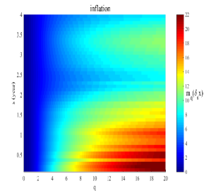
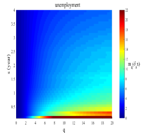
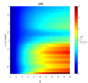
Figure 2: The colour map of the moment $m_{q}(\delta_{s}x)$ (from Eq. (5)) and joint moment $m^{joint}_{q}(\delta_{s}x_{1},\delta_{s}x_{2})$ (from Eq. (14)) for different values of $q$ and different time scale $s$. As it can be seen, for unemployment (middle figure) the value of high moments drop rapidly for scales above six months.

To improve our understanding about the behavior of the rare events, higher moments of the variables’ increments have been measured for various orders and various time scales. Recall that high moments are more influenced by the rare events in the tails of the PDF.

In Fig. 2, color intensity plot of such high moments are depicted for different time scales. As it can be seen, the value of the high moments of the unemployment rates have their largest values for scales below six months. Above six months the moments drop rapidly. In contrast to the unemployment case, the value of high moments for the inflation rates is relatively noticeable for all scales but is higher in at scales below $2$ years.

The right panel in Fig.2 illustrates that the behavior of the joint moment is more similar to the inflation case where a noticeable reduction can be observed for scales above $2$ years. This means that large fluctuations in inflation and unemployment are more strongly coupled above this time interval.

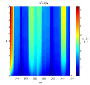
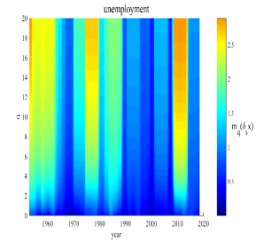
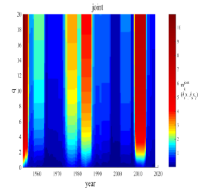
Figure 3: The moments $m_{q}(\delta_{s}x)$ and $m^{joint}_{q}(\delta_{s}x_{1},\delta_{s}x_{2})$ of order $q$ are estimated at scale 1 year from $1948$ to $2018$ for inflation (left), unemployment (middle) and the pair of variables (right).

At the next step, the behavior of high moments of inflation and unemployment are investigated as time evolved between January $1948$ and October $2018$. A window of five years is chosen and the moments $m_{q}(\delta_{s}x)$ calculated for the one year scale ($s=1$). The window is slowly moved along the time axis. Results have been depicted in Fig. 3.

As it can be seen, from the red bands, the joint relation has sharply grown at critical periods in the modern history of the US economy, i.e. the volatile postwar period, the stagflation of $70_{th}$, the period of Volcker deflationary program, in the 80’s, and the great recent recession of 2008-2009.

If the inflation rate likely dominates the coupled relation at the post WWII time, in contrast, the unemployment rate seems to dominate the joint relation in both other cases.

IV Conclusion

Inflation and unemployment are dependent variables with non-Gaussian PDFs; however, the scale and intensity of this dependency and their coupling effects have been, and are still, much debated. The controversy finds its importance when the government aims to impose an expansionary monetary policy over the economic crises. Many researchers have discussed the relation between inflation and unemployment; recall one Friedman friedman1977nobel , among others, rochon2018relationship . In this work, we were interested in large and rare fluctuations in the measures of these economic variables, in order to observe possible enhancements in themselves and in their coupling. We have focused on the non-Gaussianity of the signals’ PDFs and their coupling. The Multifractal Random Walk (MRW) is known as a good approach that detects the non-Gaussianity of PDFs through the parameter $\lambda^{2}(s)$, the variance of the log-normal process. Moreover, the bivariate Multifractal Random Walk (Bi-MRW) method is useful for analyzing two non-Gaussian stochastic processes through the corresponding variance $\Lambda^{2}(s)$.

By analysing 70 years of US data via these techniques, the non-Gaussianity of the PDFs of unemployment and inflation and also their joint relation have been detected. The non-Gaussianity parameter $\lambda^{2}(s)$ of the unemployment rate data is smaller than that for the inflation and that for the coupled relation $\Lambda^{2}(s)$. It is observed that after one year, the behavior of this parameter for the unemployment case tends toward a normal condition, but on the contrary, for the inflation data, the non-Gaussianity parameter persists for all studied scales. The non-Gaussianity of the joint relation decreases to small values for scales above $2$ years.

Also, this behavior is observable in the high-order moments of these (three) variables. Moving the observation window over time, it is discovered that the non-Gaussianities of the parameters and of their coupling substantially grow over the critical periods of the economy.

References

- (1) A.W. Phillips, The Relation between Unemployment and the Rate of Change of Money Wage Rates in the United Kingdom 1861-1957, Economica 25 (100), 283-299 (1958).
- (2) P.A. Samuelson, R.M. Solow, Analytical aspects of anti-inflation policy, American Economic Review 40, 177-194 (1960).
- (3) M. Friedman, The role of monetary policy, American Economic Review 58, 1-17 (1968).
- (4) E.S. Phelps, Money Wage Dynamics and Labor Market Equilibrium, Journal of Political Economy 76, 678-711 (1968).
- (5) J.B. Taylor, The Role of Policy in the Great Recession and the Weak Recovery, American Economic Review 104(5), 61-66 (2014).
- (6) F.S. Mishkin, Monetary policy strategy: Lessons from the crisis, NBER Working Paper, 16755 (2011).
- (7) G.A. Akerlof, W.T. Dickens, G.L. Perry, T.F. Bewley, A.S. Blinder, Near-Rational Wage and Price Setting and the Long-Run Phillips Curve, Brookings Papers on Economic Activity 31(1), 1-60 (2000).
- (8) J. Gali, M. Gertler, J.D. Lopez-Salido, Robustness of the estimates of the hybrid New Keynesian Phillips curve, Journal of Monetary Economics 52, 1107-1118 (2005).
- (9) N.G. Mankiw, R. Reis, Sticky Information versus Sticky Prices: A Proposal to Replace the New Keynesian Phillips Curve, The Quarterly Journal of Economics 117, 1295-1328 (2002).
- (10) H. Safdari, A. Hosseiny, S.V. Farahani, G.R. Jafari, A picture for the coupling of unemployment and inflation, Physica A: Statistical Mechanics and its Applications 444, 744-750, (2016).
- (11) W.B. Arthur, Complexity and the Economy, Science 284, 107–109 (1999).
- (12) D. Delli Gatti, C. Di Guilmi, E. Gaffeo, G. Giulioni, M. Gallegati, A. Palestrini, A new approach to business fluctuations: heterogeneous interacting agents, scaling laws and financial fragility, Journal of Economic Behavior & Organization 56 (4), 489-512 (2005).
- (13) A. Namaki, A.H. Shirazi, R. Raei, G.R. Jafari, Network analysis of a financial market based on genuine correlation and threshold method, Physica A: Statistical Mechanics and its Applications 390 (21-22), 3835-3841 (2011).
- (14) J.D. Farmer, M. Gallegati, C. Hommes, A. Kirman, P. Ormerod, S. Cincotti, A. Sanchez, D. Helbing, A complex systems approach to constructing better models for managing financial markets and the economy, The European Physical Journal Special Topics 214(1), 295-324 (2012).
- (15) A. Hosseiny, M. Bahrami, A. Palestrini, M. Gallegati, Metastable Features of Economic Networks and Responses to Exogenous Shocks, PLoS ONE 11(10): e0160363 (2016).
- (16) A. Namaki, R. Raei, N. Asadi, A. Hajihasani, Analysis of Iran Banking Sector by Multi-Layer Approach, Iranian Journal of Finance 3(1), 73-89 (2019).
- (17) D. Helbing, A. Kirman. Rethinking economics using complexity theory. Real-world Economics Review, 64 (2013).
- (18) F. Schweitzer, G. Fagiolo, D. Sornette, F. Vega-Redondo, A. Vespignani, D.R. White, Economic networks: The new challenges, Science 325, 422-425 (2009).
- (19) A.M. D’Arcangelis, G. Rotundo. Complex networks in finance, in Complex networks and dynamics, pp. 209-235. Springer, Cham (2016).
- (20) A.Chakraborti, D. Challet, A. Chatterjee, M. Marsili, Y.C. Zhang, B. K. Chakrabarti, Statistical mechanics of competitive resource allocation using agent-based models, Physics Reports 552, 1-25, (2015).
- (21) A. Namaki, R Raei, G.R. Jafari, Comparing Tehran stock exchange as an emerging market with a mature market by random matrix approach, International Journal of Modern Physics C 22 (4), 371-383 (2011).
- (22) A. Dragulescu, V.M. Yakovenko, Statistical mechanics of money. The European Physical Journal B-Condensed Matter and Complex Systems 17, 723-729 (2000).
- (23) N. Vandewalle, M. Ausloos, P. Boveroux, A. Minguet, How the financial crash of October 1997 could have been predicted, European Physical Journal B 4, 139-141 (1998).
- (24) A. Hosseiny, M. Gallegati, Role of intensive and extensive variables in a soup of firms in economy to address long run prices and aggregate data. Physica A: Statistical Mechanics and its Applications, 470, 51-59 (2017).
- (25) H. Aoyama, Y. Fujiwara, Y.Ikeda, H. Iyetomi, W. Souma, Econophysics and Companies: Statistical Life and Death in Complex Business Networks, Cambridge University Press, Cambridge (2010).
- (26) L.M. Varela, G. Rotundo, M. Ausloos, J. Carrete, Complex networks analysis in socio-economic models, in Complexity and Geographical Economics. Topics and Tools, P. Commendatore, S.S. Kayam and I. Kubin Eds. (Springer, 2015) pp. 209-245.
- (27) A. Hosseiny, Geometrical Imaging of the Real Gap Between Economies of China and the United States. Physica A: Statistical Mechanics and its Applications 479, 151-161 (2017).
- (28) P Anderson, Perspective: Complexity theory and organization science. Organization Science 10(3), 216-232 (1999).
- (29) K. Ivanova, H.N. Shirer, E.E. Clothiaux, N. Kitova, M.A. Mikhalev, T.P. Ackerman, M. Ausloos, A case study of stratus cloud base height multifractal fluctuations, Physica A 308, 518-532 (2002).
- (30) M. Ausloos, Generalized Hurst exponent and multifractal function of original and translated texts mapped into frequency and length time series, Physical Review E 86(3), 031108 (2012).
- (31) N. Vandewalle, M. Ausloos, Fractals in Finance, in Fractals and Beyond. Complexity in the Sciences, M.M. Novak, Ed. pp. 355-356, World Scient., Singapore (1998).
- (32) N. Vandewalle, M. Ausloos, Multi-affine analysis of typical currency exchange rates, European Physical Journal B 4, 257-261 (1998).
- (33) K. Ivanova, M. Ausloos, Low q-moment multifractal analysis of Gold price, Dow Jones Industrial Average and BGL-USD exchange rate, European Physical Journal B 8, 665-669,(1999).
- (34) D. Grech, Alternative measure of multifractal content and its application in finance, Chaos, Solitons and Fractals 88, 183–195, (2016).
- (35) W.-X. Zhou, Finite-size effect and the components of multifractality in financial volatility, Chaos, Solitons and Fractals 45(2), 147–155, (2012).
- (36) E. Bacry, J. Delour, J.F. Muzy, Multifractal random walk, Physical Review E 64(2), 026103 (2001).
- (37) Z. Koohi Lai, S. Vasheghani Farahani, S.M.S Movahed, G.R. Jafari, Coupled uncertainty provided by a multifractal random walker, Physics Letters A 379, 2284-2290 (2015).
- (38) B. Chabaud, A. Naert, J. Peinke, F. Chillá, B. Castaing, and B. Hébral, Transition towards developed turbulence, Physical Review Letters 73, 3227-3230 (1994).
- (39) S. Ghashghaie, W. Breymann, J. Peinke, P. Talkner, Y. Dodge, Turbulent cascades in foreign exchange markets. Nature 381, 767-770 (1996).
- (40) M. Ausloos, K. Ivanova, Multifractal nature of stock exchange prices, Comp. Physics Communications 147, 582-585 (2002).
- (41) J.F. Muzy, D. Sornette, J. Delour, A. Arneodo, Multifractal returns and hierarchical portfolio theory, Quantitative Finance 1(1), 131-148 (2001).
- (42) J. Muzy, J. Delour, E. Bacry, Modelling fluctuations of financial time series: from cascade process to stochastic volatility model, European Physical Journal B 17, 537–548 (2000).
- (43) F. Shayeganfar, S. Jabbari-Farouji, M. Sadegh Movahed, G.R. Jafari, M. Reza Rahimi Tabar, Multifractal analysis of light scattering-intensity fluctuations, Physical Review E 80, 061126 (2009).
- (44) http://www.usinflationcalculator.com
- (45) https://www.bls.gov/bls/unemployment.htm.
- (46) G. D’ Agostini, Bayesian Inference in Processing Experimental Data: Principles and Basic Applications, Reports on Progress in Physics 66,1383-1420 (2003).
- (47) D. S. Sivia and J. Skilling, Data Analysis: A Bayesian Tutorial, Oxford University Press (2006).
- (48) L. Ball, N.G. Mankiw, D. Romer, G.A. Akerlof, A. Rose, J. Yellen, C.A. Sims, The new Keynesian economics and the output-inflation trade-off, Brookings papers on economic activity (1), 1-82 (1988).
- (49) M. Friedman, Nobel lecture: inflation and unemployment. Journal of Political Economy, 85(3), 451-472 (1977).
- (50) L.-Ph. Rochon, S. Rossi. The relationship between inflation and unemployment: a critique of Friedman and Phelps. Review of Keynesian Economics 6(4), 533-544 (2018).