Hemispheric handedness in the Galactic synchrotron polarization foreground

Abstract

The large-scale magnetic field of the Milky Way is thought to be created by an $\alpha\Omega$ dynamo, which implies that it should have opposite handedness North and South of the Galactic midplane. Here we attempt to detect a variation in handedness using polarization data from the Wilkinson Microwave Anisotropy Probe. Previous analyzes of the parity-even and parity-odd parts of linear polarization of the global dust and synchrotron emission have focused on quadratic correlations in spectral space of, and between, these two components. Here, by contrast, we analyze the parity-odd polarization itself and show that it has, on average, opposite signs in Northern and Southern Galactic hemispheres. Comparison with a Galactic mean-field dynamo model shows broad qualitative agreement and reveals that the sign of the observed hemispheric dependence of the azimuthally averaged parity-odd polarization is not determined by the sign of $\alpha$, but by the sense of differential rotation.

1. Introduction

The main purpose of the Wilkinson Microwave Anisotropy Probe (WMAP) and Planck satellites was to map the cosmic background radiation. However, most of the polarized emission comes from the Galactic foreground (Planck Collaboration Int. XXX, 2016; Planck Collaboration XI, 2018). Removing this contribution remains an important goal in observational cosmology for the detection of primordial gravitational waves and magnetic fields. This requires a thorough understanding of the detailed foreground emission. The Galactic magnetic field is also of great interest to astroparticle physics, as it is a key factor in tracing high-energy cosmic rays to their origin. It could also be critical for understanding the hemispheric dependence of the handedness in the arrival directions of cosmic rays (Kahniashvili & Vachaspati, 2006) and, in particular, the gamma rays observed with the Fermi Large Area Telescope (Tashiro et al., 2014). The WMAP satellite data also allow us to learn new important aspects about the Galaxy (e.g. Jansson & Farrar, 2012) that have never been possible to assess systematically with conventional techniques. In particular, Galactic synchrotron and dust polarizations can reveal important information about the nature of its magnetic field that can be best understood by comparing with synthetic polarization maps form numerical simulations (Väisälä et al., 2018).

The determination of the magnetic field of the Galaxy is a difficult task. Most progress has been made by using the rotation measure (RM) of pulsars or extragalactic radio sources (Haverkorn, 2015). However, the large-scale pattern of the Galactic magnetic field is still largely unknown (e.g. Men et al., 2008). Sun et al. (2009) have shown an axisymmetric disk distribution with reversals inside the solar circle using all-sky maps at $1.4\,{\rm GHz}$ from the Dominion Radio Astrophysical Observatory and the Villa Elisa radio telescope, the K-band map from the WMAP mission, as well as the Effelsberg RM survey. Other efforts include the work by Brown et al. (2007), who used RM of extragalactic radio sources to infer an axisymmetric pattern of the disk magnetic field. A recent review of the models for the Milky Way magnetic field can be found in Boulanger et al. (2018).

Synchrotron emission from the Galaxy dominates at low microwave frequencies ($<30\,{\rm GHz}$), while thermal dust emission starts to dominate at higher frequencies ($>70\,{\rm GHz}$). Full-sky continuum maps at lower frequencies are available, for example, at $408\,{\rm MHz}$ (Haslam et al., 1982), and at $1.4\,{\rm GHz}$ (Reich & Reich, 1986). Ruiz-Granados et al. (2010) have carried out a systematic comparison of a number of Galactic magnetic field models, which were fitted to the large-scale polarization map at $22\,{\rm GHz}$.

It is believed that the Galactic magnetic field is generated by a turbulent dynamo process, which can produce both small-scale and large-scale magnetic fields at the same time. Several techniques have been devised to determine signatures of dynamo-generated magnetic fields. One such aspect concerns the twistedness of the magnetic field at large and small length scales. Twist is generally quantified by magnetic and current helicities, and various approaches have been explored to determine these quantities (Volegova & Stepanov, 2010; Junklewitz & Enßlin, 2011; Oppermann et al., 2011; Brandenburg & Stepanov, 2014; Horellou & Fletcher, 2014), which are all based on Faraday rotation. A significant uncertainty is imposed by the fact that the polarization data are only sensitive to the magnetic field orientation in the plane of the sky, but not to its direction. Under certain conditions of inhomogeneity, however, the sense of twist can be inferred from just the polarization pattern projected on the sky (Kahniashvili et al., 2014; Bracco et al., 2019; Brandenburg et al., 2019).

Magnetic fields that are generated by an $\alpha\Omega$ dynamo (Krause & Rädler, 1980) have, on average, opposite handedness North and South of the disc plane. It may therefore be possible to detect signatures of such a field by analyzing the polarization patterns of the Galaxy. Exploring this for our Galaxy is the main purpose of the present work.

The basic idea is to use the decomposition of linear polarization into its parity-even and parity-odd parts. In the analysis of the cosmic background radiation, one usually computes spectral correlations between the parity-odd polarization and the temperature. However, as already pointed out by Brandenburg (2019), even just the parity-odd polarization itself can sometimes be used as a meaningful proxy. This quantity is a pseudoscalar, similar to kinetic and magnetic helicities. This means that it changes sign when viewing the system in a mirror. A difficulty in applying it as a proxy for magnetic helicity is that the parity-odd polarization is only defined with respect to a plane, and that we can only expect a non-vanishing average if the plane is always seen only from the same side, i.e., if one side is physically distinguished from the other.

2. $E$ and $B$ polarizations

The Stokes $Q$ and $U$ linear polarization parameters change under rotation of the coordinate system. However, it is possible to transform $Q$ and $U$ into a proper scalar and a pseudoscalar, which are independent of the coordinate system. These are the rotationally invariant parity-even $E$ and parity-odd $B$ polarizations. They are given as the real and imaginary parts of the spherical harmonic expansion (Durrer, 2008)

$$E+{i}B\equiv R=\sum_{\ell=2}^{N_{\ell}}\sum_{m=-\ell}^{\ell}\tilde{R}_{\ell m}Y_{\ell m}(\theta,\phi),$$ (1)

with some truncation $N_{\ell}$ and coefficients $\tilde{R}_{\ell m}$ that are related to the spectral representation of the complex linear polarization $P=Q+{i}U$ in terms of spin-weighted spherical harmonic functions. They are given by (Kamionkowski et al., 1997; Seljak & Zaldarriaga, 1997; Zaldarriaga & Seljak, 1997)

$$\tilde{R}_{\ell m}=\int_{4\pi}(Q+{i}U)\,_{2}Y_{\ell m}^{\ast}(\theta,\phi)\,\sin\theta\,{\rm d}{}\theta\,{\rm d}{}\phi,$$ (2)

where ${}_{2}Y_{\ell m}^{\ast}(\theta,\phi)$ are the spin-2 spherical harmonics, $\theta$ is colatitude, and $\phi$ is longitude. We choose $N_{\ell}=48$ for the spherical harmonic truncation. This results in some corresponding smoothing, making it easier to discern large-scale patterns in the resulting $E$ and $B$ polarizations.

It should be noted that Zaldarriaga & Seljak (1997) use another sign convention; see their Equation (6), which corresponds to a minus sign in Equation (1). Here we use Equation (5.10) of Durrer (2008); see the corresponding discussion by Brandenburg (2019) and Prabhu et al. (2020).

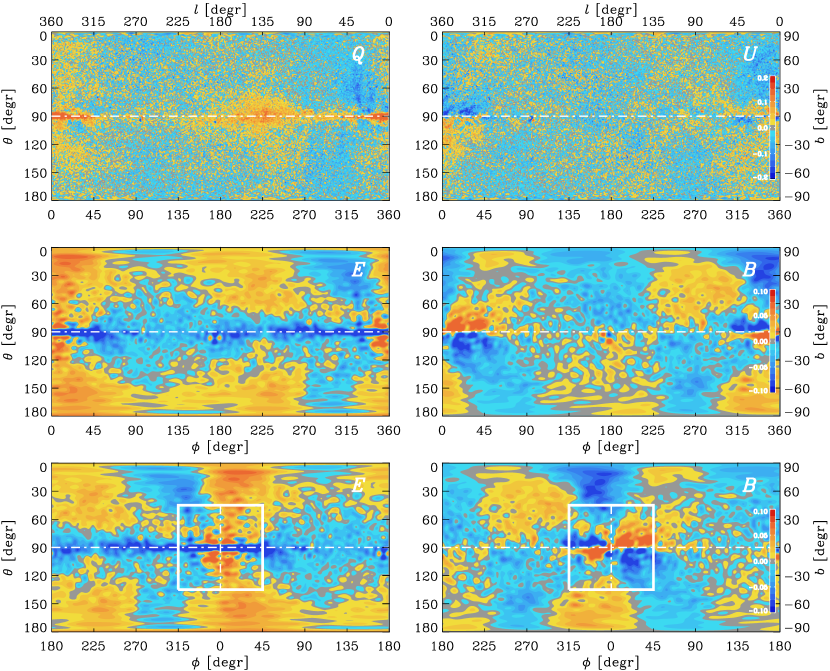
Figure 1.— Polarization results for the Galaxy. Top: $Q(\theta,\phi)$ and $U(\theta,\phi)$ in mK. Galactic $(l,b)$ coordinates are indicated on the outer axes. Middle: $E(\theta,\phi)$ and $B(\theta,\phi)$ in mK. Bottom: same as middle panels, but shifted such that the Galactic center is in the middle. Note that $\theta$ increases downward, so North (South) is at the top (bottom).

Following Vasil et al. (2016, 2018), we compute the spin-weighted spherical harmonics using Jacobi polynomials $P_{\ell}^{(a,b)}(\cos\theta)$ as

$${}_{s}Y_{\ell m}(\theta,\phi)=N_{\ell\,m}^{s}\sin^{a}(\textstyle{\theta\over 2})\cos^{b}(\textstyle{\theta\over 2})\,P_{\ell-\ell_{0}}^{(a,b)}(\cos\theta)\,e^{{i}m\phi},$$ (3)

where $a=|m+s|$, $b=|m-s|$, and

$$N_{\ell\,m}^{s}=(-1)^{\max(m,-s)}\sqrt{\frac{(2\ell+1)(\ell+\ell_{0})!(\ell-\ell_{0})!}{4\pi(\ell+\ell_{1})!(\ell-\ell_{1})!}}$$ (4)

is a normalization factor with $\ell_{0}=\max(|m|,|s|)$ and $\ell_{1}=\min(|m|,|s|)$. Equation (4) differs from that of Vasil et al. (2018) by a factor $\sqrt{2\pi}$ to conform with the normalization of Goldberg et al. (1967).

3. Data selection and analysis

Our analysis is based on the K-band (equivalent to $22\,{\rm GHz}$) polarization data obtained by the WMAP satellite after the full nine years of operation (Bennett et al., 2013). This data can be downloaded from the LAMBDA website in the HEALPIX format (Górski et al., 2005).

In the K-band, the emission is entirely dominated by Galactic synchrotron emission, with spinning dust, thermal dust, and the CMB being sub-dominant (Bennett et al., 2013). Thus, this band is best to study the Galactic magnetic field.

The first two panels of Figure 1 show the all-sky Stokes $Q$ and $U$ maps at $22\,{\rm GHz}$ using the HEALPIX resolution parameter $N_{\rm side}=512$ (which corresponds to a pixel size of $6.8$ arcmin). We mapped this data onto a uniform grid of standard spherical coordinates, $(\theta,\phi)$, where $\theta$ is colatitude and $\phi$ is longitude, which increases eastward (using the interpolation function in the HEALPY PYTHON package). We also use Galactic coordinates $(l,b)$, where $l=360\hbox{${}^{\circ}$}-\phi$ is Galactic longitude and $b=90\hbox{${}^{\circ}$}-\theta$ is Galactic latitude (e.g. Page et al., 2007). The Galactic latitude $b$ is not to be confused with the components of the magnetic field, which will be denoted by the bold face symbol $\bm{b}_{\perp}$ so as not to confuse them with the parity-odd constituent $B$ of the linear polarization.

4. Results

4.1. Global $E$ and $B$ polarization for the Galaxy

In Figure 1, we show images of $Q$ and $U$ along with the rotationally invariant counterparts $E$ and $B$ as functions of $\theta$ and $\phi$. We see that $Q$ is mostly positive near the midplane and has maxima at $\phi=0$ and $225\hbox{${}^{\circ}$}$. Near $\phi=0$, $U$ is positive (negative) in the Southern (Northern) hemisphere. The $E$ polarization has negative extrema at $\phi\approx 90\hbox{${}^{\circ}$}$ and $270\hbox{${}^{\circ}$}$, and is positive at intermediate longitudes and also at high Galactic latitudes. Around the Galactic center, the $B$ polarization has a characteristic cloverleaf-shaped pattern, which is best seen in the recentered lower panels of Figure 1; see the white box. This is similar to what was reported in the appendix of Brandenburg & Furuya (2020). This pattern is the result of the $B$-decomposition of a purely vertical magnetic field near the Galactic center.

To study the systematic latitudinal dependence more clearly, we show in Figure 2 the $\phi$-averaged profiles of $Q$, $U$, $E$, and $B$, which we denote by angle brackets with subscript $\phi$, i.e., $\langle Q\rangle_{\phi}=\int_{0}^{2\pi}Q\,{\rm d}{}\phi/2\pi$, and likewise for the other quantities. We also show the standard deviation and statistical error of the mean, where we took data that are separated by more than $10\hbox{${}^{\circ}$}$ as statistically independent. We clearly see that, near the equatorial plane ($\theta=90\hbox{${}^{\circ}$}$), $\langle Q\rangle_{\phi}$ and $\langle E\rangle_{\phi}$ have a similar symmetric $\theta$ dependence about $\theta=90\hbox{${}^{\circ}$}$, but with opposite signs. Also $\langle U\rangle_{\phi}$ and $\langle B\rangle_{\phi}$ have opposite signs relative to each other, but both are roughly antisymmetric about $\theta=90\hbox{${}^{\circ}$}$. There is, however, a negative (positive) spike in $\langle U\rangle_{\phi}$ ($\langle B\rangle_{\phi}$) at $\theta=90\hbox{${}^{\circ}$}$. It may be associated with an imperfect cancelation of the cloverleaf-shaped feature at the Galactic center.

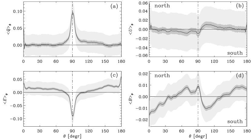
Figure 2.— Azimuthally averaged polarization results for the Galaxy. Top: $\langle Q\rangle_{\phi}(\theta)$ and $\langle U\rangle_{\phi}(\theta)$. Bottom: $\langle E\rangle_{\phi}(\theta)$ and $\langle U\rangle_{\phi}(\theta)$. The statistical error of the mean and the standard deviation are indicated by dark and light shades, respectively.

It should be noted here that the use of azimuthal averages breaks the rotational invariance under coordinate transformations. This is why the azimuthal average $\langle E\rangle_{\phi}$ depends solely on $\langle Q\rangle_{\phi}$, and $\langle B\rangle_{\phi}$ depends solely on $\langle U\rangle_{\phi}$.

Table 1 First few expansion coefficients of Equation (1).

$m$ $\mu$ $\kappa$ $\kappa\tilde{E}_{2\,m}^{(\mu)}$ $\kappa\tilde{E}_{4\,m}^{(\mu)}$ $\kappa\tilde{B}_{3\,m}^{(\mu)}$ $\kappa\tilde{B}_{5\,m}^{(\mu)}$ 0 K 1000 $56$ $-34$ $\mathbf{-18}$ $6$ Q 5000 $45$ $-27$ $\mathbf{-35}$ $10$ A 0.1 $73$ $-22$ $\mathbf{-0.038}$ $-0.002$ B 0.1 $92$ $-34$ $\mathbf{+0.014}$ $-0.13$ C 5000 $68$ $-27$ $\mathbf{-7}$ $+8$ D 0.1 $73$ $-22$ $\mathbf{+0.038}$ $+0.002$ 1 K 1000 $1-9{i}$ $4+17{i}$ $4+{i}$ $8-5{i}$ Q 5000 $1-8{i}$ $-{i}$ $-10-2{i}$ $2{i}$ A 0.1 $1$ $1$ $-4{i}$ ${i}$ B 0.1 $-41-{i}$ $13$ $12{i}$ $-5{i}$ C 5000 $57+5{i}$ $-15-8{i}$ $-2-36{i}$ $2+9{i}$ D 0.1 $1$ $1$ $-4{i}$ ${i}$ 2 K 1000 $7-8{i}$ $9-22{i}$ $-20-17{i}$ $-13+5{i}$ Q 5000 $-1-7{i}$ $-15{i}$ $-13$ $-9$ A 0.1 $41+3{i}$ $-4$ $2-26{i}$ $5{i}$ B 0.1 $28+2{i}$ $-5$ $1-10{i}$ $-2{i}$ C 5000 $31+4{i}$ $12-4{i}$ $5-50{i}$ $-7+13{i}$ D 0.1 $41+4{i}$ $-4$ $3-26{i}$ $-1+5{i}$

The full sky maps of $E$ and $B$ in Figure 1 yield a prominent $m=2$ variation with odd symmetry about the equator. The odd $m=0$ variation cannot be seen without azimuthal averaging. To quantify the relative importance of the $m=0$ and $2$ contributions, we list in Table LABEL:Tsummary the first few coefficients $\tilde{E}_{\ell m}=(\tilde{R}_{\ell m}+\tilde{R}_{\ell,\,-m}^{\ast})/2$ and $\tilde{B}_{\ell m}=(\tilde{R}_{\ell m}-\tilde{R}_{\ell,\,-m}^{\ast})/2{i}$, which is opposite to the sign convention of Seljak & Zaldarriaga (1997) for $E$ and $B$. To assess the robustness of the result, we also compare with WMAP data in the Q-band (41 GHz). We distinguish the two bands by superscripts K and Q; see Brandenburg & Brüggen (2020) for the full set of coefficients. We also compare with simulation data (superscripts A–D) discussed in Sect. 4.2.3. The hemispheric handedness is quantified by the coefficients $\tilde{B}_{3\,0}^{(\mu)}$, which are negative, except for the models $\mu={\rm B}$ and D discussed in Sect. 4.2.3.

4.2. Comparison with a Galactic dynamo model

4.2.1 Review of the model

To see how our results compare with a Galactic mean field dynamo model, we analyze the model of Brandenburg & Furuya (2020), which was recently applied to assess the parity-even and parity-odd polarizations for an edge-on view of the galaxy NGC 891. In the present work, however, we use the same model to compute a view from the position of the Sun, located in the mid-plane $8\,{\rm kpc}$ from the Galactic center ($\mu={\rm A}$). We also compare with $3\,{\rm kpc}$ distance ($\mu={\rm B}$), and how models with opposite signs of the $\alpha$ effect ($\mu={\rm C}$) and both $\alpha$ and $\Omega$ ($\mu={\rm D}$).

The models have parameters similar to that of Brandenburg et al. (1993), which was designed to describe the halo magnetic field of NGC 891. The vertical wind in the model of Brandenburg et al. (1993) was omitted.

We adopt a Cartesian domain of size $20\times 20\times 5\,{\rm kpc}^{3}$ with normal field boundary conditions. The computations are performed with the Pencil Code (Brandenburg & Dobler, 2010) using $256\times 256\times 64$ meshpoints.

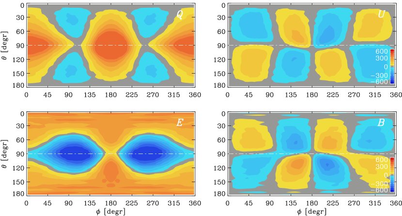
Figure 3.— Polarization results for the mean-field model with the Faraday rotation term in Equation (6) included. Top: $Q(\theta,\phi)$ and $U(\theta,\phi)$. Bottom: $E(\theta,\phi)$ and $B(\theta,\phi)$.

The distribution of the $\alpha$ effect in the model has a radius of $15\,{\rm kpc}$ and a height of $1.5\,{\rm kpc}$. In Brandenburg et al. (1993), this height was associated with the thick disk (Reynolds layer). For the rotation curve, a Brandt profile was assumed with an angular velocity of $\Omega_{0}=75\,{\rm Gyr}^{-1}$ and a turnover radius of $\varpi_{\Omega}=3\,{\rm kpc}$, where the rotation law attains constant linear velocity with $V_{0}=\Omega_{0}\varpi_{\Omega}\approx 225\,{\rm km\,s}^{-1}$. The $\alpha$ effect has a strength of $\alpha_{0}=22\,{\rm km}\,{\rm s}^{-1}$ near the axis, but declines with increasing distance from the axis and has $8\,{\rm km\,s}^{-1}$ at $\varpi=8\,{\rm kpc}$. It is also reduced locally by $\alpha$ quenching, which limits the mean field to about $10\,\mu{\rm G}$. The resulting magnetic field has quadrupolar symmetry with respect to the midplane, i.e., the sign of the toroidal field is the same above and below the midplane.

4.2.2 Computation of the polarization

To compute the apparent magnetic field from the position of the Sun in our model, we set up a local spherical coordinate system to inspect the local emission from a sphere around the observer at the position $\bm{r}_{0}\equiv(x_{0},y_{0},z_{0})$ in the direction $\hat{\bm{n}}$, where $\hat{\bm{n}}$ is the unit vector of $\bm{r}-\bm{r}_{0}$, with $\bm{r}$ being the position of a point on the sphere around the observer, and $s=|\bm{r}-\bm{r}_{0}|$ the distance. The cylindrical radius around the observer is $\varpi=|\mbox{\boldmath$\varpi$}{}|$, where $\mbox{\boldmath$\varpi$}{}=(x-x_{0},y-y_{0},0)$, which allows us to compute the local azimuthal unit vector as $\hat{\bm{\phi}}=\hat{\mbox{\boldmath$z$}}{}\times\bm{\hat{\varpi}}$, where $\bm{\hat{\varpi}}=\mbox{\boldmath$\varpi$}{}/\varpi$ and $\hat{\mbox{\boldmath$z$}}{}=(0,0,1)$ are the cylindrical and vertical unit vectors, respectively. The third coordinate direction in our local coordinate system is colatitude with the unit vector $\bm{\hat{\theta}}=\hat{\bm{\phi}}\times\hat{\bm{n}}$. The polarization on the unit sphere of the observer is then computed from $\bm{b}_{\perp}=(b_{\theta},b_{\phi})$, whose components are given by $b_{\theta}=\bm{b}\cdot\bm{\hat{\theta}}$ and $b_{\phi}=\bm{b}\cdot\hat{\bm{\phi}}$.

For given wavelength, the synchrotron emissivity is $\propto n_{\rm CR}|\bm{b}_{\perp}|^{\sigma}$, where $\sigma\approx 1.9$ (Ginzburg & Syrovatskii, 1965). In the following, we assume $\sigma=2$, so that the emissivity in the complex polarization can simply be written as

$$P_{\rm intr}(s,\theta,\phi)=-\epsilon_{0}\,n_{\rm CR}(b_{\theta}+{i}b_{\phi})^{2},$$ (5)

where $\epsilon_{0}$ is a positive constant, $n_{\rm CR}$ is the cosmic ray electron density, and $s$ is the distance from the observer. The minus sign in Equation (5) reflects the fact that the polarization plane represents the electric field vector of the radiation which is orthogonal to the magnetic field in the plane of the sky.

We compute the observable complex polarization along the line of sight as

$$P(\theta,\phi)=\int_{0}^{\infty}P_{\rm intr}\,e^{2{i}b_{r}/b_{\rm F}}\,{\rm d}{}s,$$ (6)

where $b_{\rm F}=(k_{\rm F}n_{\rm e}\lambda^{2}s)^{-1}$, with $k_{\rm F}=2.6\times 10^{-17}\,{\rm G}^{-1}$ being a constant (e.g. Pacholczyk, 1970), $n_{\rm e}$ the thermal electron density, and $\lambda$ the wavelength. Absorption can safely be neglected for our purposes. For the sake of illustration, we adopt Gaussian profiles for thermal and cosmic ray electron densities, $n_{\rm e}=n_{\rm e0}\exp(-z^{2}/2H_{\rm e}^{2})$ and $n_{\rm CR}=n_{\rm CR0}\exp(-z^{2}/2H_{\rm CR}^{2})$, with $H_{\rm e}=H_{\rm CR}=1\,{\rm kpc}$ and midplane values $n_{\rm e0}$ and $n_{\rm CR0}$ for the electron densities. For $\lambda=1.36\,{\rm cm}$ (corresponding to $22\,{\rm GHz}$), $n_{\rm e0}=0.03\,{\rm cm}^{-3}$, and $s=1\,{\rm kpc}$, we have $b_{\rm F}=230\,\mu{\rm G}$. This is large compared to the typical Galactic magnetic field strength of a few $\,\mu{\rm G}$, so Faraday rotation effects are weak. We perform the line-of-sight integration by computing $P(\theta,\phi)$ on a $(\theta,\phi)$ mesh with $36\times 72$ meshpoints for distances $s$ from the observer going up to $5\,{\rm kpc}$ in steps of $\Delta s=0.2\,{\rm kpc}$.

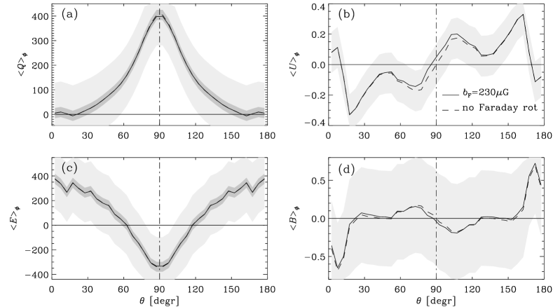
Figure 4.— Azimuthally averaged polarization results for the mean-field model with Faraday rotation using $b_{\rm F}=230\,\mu{\rm G}$ (solid lines) and without Faraday rotation (dashed lines). Top: $\langle Q\rangle_{\phi}(\theta)$ and $\langle U\rangle_{\phi}(\theta)$. Bottom: $\langle E\rangle_{\phi}(\theta)$ and $\langle B\rangle_{\phi}(\theta)$. The statistical error of the mean and the standard deviation are indicated by dark and light shades, respectively, except for panels (b) and (d), where only the former is shown.

4.2.3 Results from the mean-field model

In Figure 3 we show the results for Model B of Brandenburg & Furuya (2020). In spite of the parameters being unrealistic for the Galaxy, there are characteristic features that are similar to what is seen in Figure 1 for the Galaxy: positive $Q$ at $\phi=0$ and $180\hbox{${}^{\circ}$}$, along with negative $E$ at $\phi=90\hbox{${}^{\circ}$}$ and $270\hbox{${}^{\circ}$}$. The results for $U$ and $B$ are not immediately obvious because there are two nearly equally big patches of opposite sign in each hemisphere. Only after $\phi$-averaging do we recognize a latitudinal dependence that is similar to that of the Galaxy; see Figure 4. The observed sign of $\tilde{B}_{3\,0}^{(\mu)}$ emerges only when we place the observer at a distance sufficiently far away from the Galactic center ($\mu={\rm A}$), while for smaller distances ($\mu={\rm B}$), the sign changes and the $\langle B\rangle_{\phi}(\theta)$ profile becomes similar to that shown in the top–right panel of Figure 1 of Brandenburg (2019). Faraday rotation is weak, but it contributes a profile that is symmetric about the equator. This is because the global magnetic field has quadrupolar symmetry; see Brandenburg (2019) for a corresponding result for a dipolar field. Changing the sign of $\alpha_{0}$ results in a qualitatively different (oscillatory) dynamo, but, to our surprise, it does not change the sign of $\tilde{B}_{3\,0}^{(\mu)}$. The sign only changes when the differential rotation changes and thereby the global Galactic spiral. Changing the signs of $\alpha_{0}$ and $\Omega_{0}$ simultaneously has the advantage of leaving the dynamo properties unchanged.

An important difference between model and observation is the fact that in our model, the amplitude of $\langle B\rangle_{\phi}(\theta)$ is several hundred times smaller than that of $\langle E\rangle_{\phi}(\theta)$, while for the Galaxy, it is only about ten times smaller; see Table LABEL:Tsummary. We recall that the quadratic $EE$ correlation was found to be about twice that of the $BB$ correlation (Planck Collaboration Int. XXX, 2016). This came as a major surprise (Kandel et al., 2017) and triggered numerous investigations trying to explain this (Kritsuk et al., 2018). In the present paper, however, we have not studied quadratic correlations, but the signed functions $E$ and $B$ themselves.

5. Conclusions

The most important result from our work is Figure 2(d). Except for the spike at the equator, we see a clear hemispheric dependence of the longitudinally averaged parity-odd $B$ polarization. This shows that the magnetic field in North and South, which is responsible for the polarization pattern, must be mirror images of each other, statistically speaking. To our knowledge, this is the first time that such a clear measurement of handedness has ever been made for the Galaxy. Remarkably, the results obtained for the mean-field dynamo agree qualitatively with those for the Galaxy, although the signal is much weaker in the model; see Figure 4(d).

To interpret our results further, we must learn how to decipher the $B$ signal. There is no one-to-one correspondence between $B$ polarization and magnetic helicity. Indeed, $B$ can be zero even for fully helical turbulence (Brandenburg et al., 2019; Bracco et al., 2019). We only obtain a finite signal if one viewing direction is preferred over another, as was discussed in those two papers. Whether or not this argument actually works for the Galaxy is not a priori clear because the $\alpha$ effect produces magnetic helicity of opposite signs at large and small scales. In the Sun, for example, observations of active regions tend to reveal only the small-scale contribution (Prabhu et al., 2020). Our present paper now shows that this may be different for the Galaxy. Beck et al. (2019) emphasized, however, that much of the Galactic polarized emission is caused by a turbulent anisotropic component, which Jansson & Farrar (2012) called stiated. It is therefore plausible that the detected hemispheric handedness is caused by the opposite orientations of the Galactic spiral in the two hemispheres; see the reversed sign of $\tilde{B}_{3\,0}^{(\mu)}$ for $\mu={\rm D}$ in Table LABEL:Tsummary.

Our paper reveals a number of other properties in the $(\theta,\phi)$ maps of $E$ and $B$ that also agree qualitatively with the dynamo model: negative extrema of $E$ at the equator near $\phi=90\hbox{${}^{\circ}$}$ and $270\hbox{${}^{\circ}$}$, and two positive (negative) extrema of $B$ at $\phi=45\hbox{${}^{\circ}$}$ and $225\hbox{${}^{\circ}$}$ in the North (South). However, the sign of the azimuthally-averaged $B$ appears not to be related to the sign of the $\alpha$ effect, as was originally hoped, but it seems to reflect the spiral nature of the Galaxy. Looking South gives a mirror image of the Galactic spiral compared to the view towards North. This new finding is supported by considering the quantity $\tilde{B}_{3\,0}$ in our models.

References

- Beck et al. (2019) Beck, R., Chamandy, L., Elson, E., & Blackman, E. G. 2019, Galaxies, 8, 4
- Bennett et al. (2013) Bennett, C. L., Larson, D., Weiland, J. L., Jarosik, N., Hinshaw, G., et al. 2013, ApJS, 208, 20
- Boulanger et al. (2018) Boulanger, F., Enßlin, T., Fletcher, A., Girichides, P., Hackstein, S., Haverkorn, M., Hörandel, J. R., Jaffe, T., Jasche, J., Kachelrieß, Michael, K., Kumiko, Pfrommer, C., Rachen, J. P., Rodrigues, L. F. S., Ruiz-Granados, B., Seta, A., Shukurov, A., Sigl, G., Steininger, T., Vacca, V., et al. 2018, JCAP, 08, 049
- Bracco et al. (2019) Bracco, A., Candelaresi, S., Del Sordo, F., & Brandenburg, A. 2019, A&A, 621, A97
- Brandenburg (2019) Brandenburg, A. 2019, ApJ, 883, 119
- Brandenburg & Brüggen (2020) Brandenburg, A., & Brüggen, B. 2020, Data sets to “Hemispheric handedness in the Galactic synchrotron foreground” (v2020.05.24.), Zenodo, doi:10.5281/zenodo.3841900.
- Brandenburg & Dobler (2010) Brandenburg, A., & Dobler, W., Pencil Code, http://ui.adsabs.harvard.edu/abs/2010ascl.soft10060B DOI:10.5281/zenodo.2315093.
- Brandenburg & Furuya (2020) Brandenburg, A., & Furuya, R. S. 2020, MNRAS, submitted, arXiv:2003.07284
- Brandenburg & Stepanov (2014) Brandenburg, A., & Stepanov, R. 2014, ApJ, 786, 91
- Brandenburg et al. (2019) Brandenburg, A., Bracco, A., Kahniashvili, T., Mandal, S., Roper Pol, A., Petrie, G. J. D., & Singh, N. K. 2019, ApJ, 870, 87
- Brandenburg et al. (1993) Brandenburg, A., Donner, K. J., Moss, D., Shukurov, A., Sokoloff, D. D., & Tuominen, I. 1993, A&A, 271, 36
- Brown et al. (2007) Brown, J. C., Haverkorn, M., Gaensler, B. M., Taylor, A. R., Bizunok, N. S., McClure-Griffiths, N. M., Dickey, J. M., & Green, A. J. 2007, ApJ, 663, 258
- Durrer (2008) Durrer, R. 2008, The Cosmic Microwave Background (Cambridge: Cambridge University Press)
- Ginzburg & Syrovatskii (1965) Ginzburg, V. L., & Syrovatskii, S. I. 1965, ARA&A, 3, 297
- Goldberg et al. (1967) Goldberg, J. N., Macfarlane, A. J., Newman, E. T., Rohrlich, F., & Sudarshan, E. C. G. 1967, JMP, 8, 2155
- Górski et al. (2005) Górski, K. M., Hivon, E., Banday, A. J., Wandelt, B. D., Hansen, F. K., Reinecke, M., Bartelmann, M. 2005, ApJ, 622, 759
- Haslam et al. (1982) Haslam, C. G. T., Salter, C. J., Stoffel, H., & Wilson, W. E. 1982, A&AS, 47, 1
- Haverkorn (2015) Haverkorn, M. 2015, in Magnetic fields in diffuse media, ed. E. de Gouveia Dal Pino & A. Lazarian (Astrophys. Spa. Sci. Lib., Vol. 407, Springer), 483
- Horellou & Fletcher (2014) Horellou, C., & Fletcher, A. 2014, MNRAS, 441, 2049
- Jansson & Farrar (2012) Jansson, R., & Farrar, G. R. 2012, ApJ, 757, 14
- Junklewitz & Enßlin (2011) Junklewitz, H., & Enßlin, T. A. 2011, A&A, 530, A88
- Kahniashvili & Vachaspati (2006) Kahniashvili, T., & Vachaspati, T. 2006, PhRvD, 73, 063507
- Kahniashvili et al. (2014) Kahniashvili, T., Maravin, Y., Lavrelashvili, G., & Kosowsky, A. 2014, PhRvD, 90, 083004
- Kamionkowski et al. (1997) Kamionkowski, M., Kosowsky, A., & Stebbins, A. 1997, PhRvL, 78, 2058
- Kandel et al. (2017) Kandel, D., Lazarian, A., & Pogosyan, D. 2017, MNRAS, 472, L10
- Krause & Rädler (1980) Krause, F., & Rädler, K.-H. 1980, Mean-field Magnetohydrodynamics and Dynamo Theory (Oxford: Pergamon Press)
- Kritsuk et al. (2018) Kritsuk, A. G., Flauger, R., & Ustyugov, S. D. 2018, PhRvL, 121, 021104
- Men et al. (2008) Men, H., Ferrière, K., & Han, J. L. 2008, A&A, 486, 819
- Oppermann et al. (2011) Oppermann, N., Junklewitz, H., Robbers, G., & Enßlin, T. A. 2011, A&A, 530, A89
- Pacholczyk (1970) Pacholczyk, A. G. 1970, Radio astrophysics (Freeman, San Francisco)
- Page et al. (2007) Page, L., Hinshaw, G., Komatsu, E., Nolta, M. R., Spergel, D. N., et al. 2007, ApJS, 170, 335
- Planck Collaboration Int. XXX (2016) Planck Collaboration Int. XXX. 2016, A&A, 586, A133
- Planck Collaboration XI (2018) Planck Collaboration XI. 2018, A&A, DOI:10.1051/0004-6361/201832618, arXiv:1801.04945
- Prabhu et al. (2020) Prabhu, A., Brandenburg, A., Käpylä, M. J., & Lagg, A. 2020, A&A, submitted, arXiv:2001.10884
- Reich & Reich (1986) Reich, P., & Reich, W. 1986, A&AS, 63, 205
- Ruiz-Granados et al. (2010) Ruiz-Granados, B., Rubiño-Mart n, J. A., & Battaner, E. 2010, A&A, 522, 73
- Seljak & Zaldarriaga (1997) Seljak, U., & Zaldarriaga, M. 1997, PhRvL, 78, 2054
- Sun et al. (2009) Sun, X. H., Reich, W., Waelkens, A., & Enßlin, T. A. 2008, A&A, 477, 573
- Tashiro et al. (2014) Tashiro, H., Chen, W., Ferrer, F., & Vachaspati, T. 2014, MNRAS, 445, L41
- Väisälä et al. (2018) Väisälä, V., Gent, F. A., Juvela, M., & Käpylä, M. J. 2018, A&A, 614, A101
- Vasil et al. (2016) Vasil, G. M., Burns, K. J., Lecoanet, D., Olver, S., Brown, B. P., & Oishi, J. S. 2016, JCoPh, 325, 53
- Vasil et al. (2018) Vasil, G., Lecoanet, D., Burns, K., Oishi, J., & Brown, B. 2018, JCoPh, submitted, arXiv:1804.10320
- Volegova & Stepanov (2010) Volegova, A. A., & Stepanov, R. A. 2010, Sov. Phys. JETP, 90, 637
- Zaldarriaga & Seljak (1997) Zaldarriaga, M. & Seljak, U. 1997, PhRvD, 55, 1830