On the origins of Riemann-Hilbert problems in mathematics

Abstract.

This article is firstly a historic review of the theory of Riemann-Hilbert problems with particular emphasis placed on their original appearance in the context of Hilbert’s 21st problem and Plemelj’s work associated with it. The secondary purpose of this note is to invite a new generation of mathematicians to the fascinating world of Riemann-Hilbert techniques and their modern appearances in nonlinear mathematical physics. We set out to achieve this goal with six examples, including a new proof of the integro-differential Painlevé-II formula of Amir, Corwin, Quastel [ACQ] that enters in the description of the KPZ crossover distribution. Parts of this text are based on the author’s Szegő prize lecture at the $15$th International Symposium on Orthogonal Polynomials, Special Functions and Applications (OPSFA) in Hagenberg, Austria.

1. Introduction

Riemann-Hilbert problems, in short RHPs, are useful in the analysis of orthogonal polynomials (OP), special functions (SF) and thus several applications (A) in mathematics or physics. Still, these modern appearances of RHPs are quite detached from the original meaning of the term RHP and it is our primary objective to pin down the occurrence of the first problem in mathematics that was coined a RHP. Once done, we will follow Plemelj’s traces whose work on the original RHP gave rise to an analytic apparatus, the Riemann-Hilbert techniques or Riemann-Hilbert methods, which found various applications in the OPSFA realm. We will showcase and advertise the latter modern aspects of the theory with examples from mathematical physics, in particular examples from nonlinear wave and integrable systems theory, statistical mechanics, random matrix theory and integrable probability.

2. The original Riemann-Hilbert problem

In order to answer the question “What is $\ldots$ a Riemann-Hilbert problem” one should go back to 1900, the year of the second international congress of mathematics. Held at the turn of the century in Paris, the ICM 1900 proved to be highly influential for the development of 20th century mathematics, in particular since Hilbert delivered his famous address in the section Bibliographie et Histoire. Enseignement et methodes. During his lecture he presented (because of time constraints) ten mathematical problems “from the discussion of which an advancement of science may be expected”, see [H, page $445$]. The full, twenty-three long, list of Hilbert’s problems appeared in German print even before the French proceedings of the congress. Scrolling through this list we eventually encounter problem $\#21$, the main focus point of this section, cf. [H0, page 289-290]:

21. Beweis der Existenz linearer Differentialgleichungen mit vorgeschriebener Monodromiegruppe

Aus der Theorie der linearen Differentialgleichungen mit einer unabhängigen Veränderlichen $z$ möchte ich auf ein wichtiges Problem hinweisen, welches wohl bereits Riemann im Sinne gehabt hat, und welches darin besteht, zu zeigen, daß es stets eine lineare Differentialgleichung der Fuchsschen Klasse mit gegebenen singulären Stellen und einer gegebenen Monodromiegruppe giebt. Die Aufgabe verlangt also die Auffinding von $n$ Functionen der Variabeln $z$, die sich überall in der complexen $z$-Ebene regulär verhalten, außer etwa in den gegebenen singulären Stellen: in diesen dürfen sie nur von endlich hoher Ordnung unendlich werden und beim Umlauf der Variabeln $z$ um dieselben erfahren sie die gegebenen linearen Substitutionen. Die Existenz solcher Differentialgleichungen ist durch Constantenzählung wahrscheinlich gemacht worden, doch gelang der strenge Beweis bisher nur in dem besonderen Falle, wo die Wurzeln der Fundamentalgleichungen der gegebenen Substitutionen sämtlich vom absoluten Betrage 1 sind. Diesen Beweis hat L. Schlesinger auf Grund der Poincaréschen Theorie der Fuchsschen $\zeta$-Functionen erbracht. Es würde offenbar die Theorie der linearen Differentialgleichungen ein wesentlich abgeschlosseneres Bild zeigen, wenn die allgemeine Erledigung des bezeichneten Problems gelänge.

In this problem Hilbert asks the reader to show that there always exists a linear differential equation of the Fuchsian class, with given singular points and monodromic group. Before reviewing some of the necessary background material in Section 3 below it will be important to point out the following peculiar wording in Hilbert’s original formulation: The problem requires the production of $n$ functions of the variable $z$, regular throughout the complex $z$ plane except at the given singular points; at these points the functions may become infinite of only finite order. Thus, Hilbert does not use the word pole singularity - he refers to what is nowadays called a regular singularity, cf. [IY, Definition $16.2$] - and he also never speaks of Fuchsian linear systems. These subtleties in the formulation of the problem played an important role as we will soon learn.

Right now we follow Anosov and Bolibrukh [AB, page $7$] and coin Hilbert’s 21st problem the original RHP: Hilbert formulated it and he explicitly mentions Riemann in his wording as this problem is extremely close to Riemann’s ideas (namely the global construction of a function from given local analytic data, i.e. the singularity locations and associated monodromy). In short,

Riemann-Hilbert Problem 2.1 (The original RHP ([H0], 1900)).

Proof of the existence of linear differential equations having a prescriped monodromic group.

This problem seems quite different from the modern RHPs discussed in Section 6 below, yet it is this problem on which the modern theory is based upon. Thus, being so influential, it is only natural to ask if RHP 2.1 has been solved $120$ years after Hilbert’s address? Well, according to the Encyclopedia of Mathematics [e], the “solution is negative or positive depending on how the problem is understood”. This answer points at a curious mathematical misunderstanding which persisted from 1908 till 1983 and which relates to the aforementioned atypicalities in Hilbert’s wording. Indeed, we highlight two possible sources of confusion:

$\diamond$ equation vs. system: The monodromy of a $p\textnormal{th}$ order scalar linear ODE with solution $y$ matches the monodromy of the $p\times p$ linear ODE system which the vector $(y,y^{\prime},\ldots,y^{p-1})$ solves. Still, at the time of the congress, cf. [P], it was known that Hilbert’s question for scalar Fuchsian equations has a negative solution unless additional singularities are included. So by a $p\textnormal{th}$ order scalar Fuchsian equation, Hilbert likely meant a generic $p\times p$ Fuchsian system.

$\diamond$ regular singularities vs. Fuchsian singularities: Both notions exist for $p\textnormal{th}$ order scalar linear ODEs in the complex plane. Although up front different in appearance, these notions are in fact equivalent (this is a result by Fuchs from 1868, cf. [IY, Theorem $19.20$]). However, this is no longer the case when one considers the same singularities for $p\times p$ linear ODE systems, see Section 4.

In turn we could think of at least three different interpretations of RHP 2.1: Given a monodromy group with encoded singularity locations, are we asked to realize it by

1. a Fuchisan linear $p\textnormal{th}$ order differential equation?

2. a linear $p\times p$ system having only regular singularities?

3. a Fuchsian system on the whole Riemann sphere $\mathbb{CP}^{1}$?

The answer to (1) is negative as shown by Poincaré [P]: the number of parameters in a $p\textnormal{th}$ order linear Fuchsian equation with singularities $a_{1},\ldots,a_{n}$ is less than the dimension of the space $\mathcal{M}$ of monodromy representations. Number (2) was positively solved by Plemelj in 1908 [P0] and believed to settle (3) as well. This belief persisted for 75 years until Kohn [K] and Arnold, Il’yashenko [AI] discovered a serious gap in Plemelj’s argument. As it turned out, interpretation (3) is much more subtle and a negative answer to Hilbert’s 21st problem in said context was eventually given by Bolibrukh in 1989, cf. [BO1, BO2]. We will now discuss in detail interpretations (2), (3) and highlight the pioneering work of Plemelj in this context. His contributions laid the foundation for several aspects of modern Riemann-Hilbert theory which we showcase through a series of OPSFA-type examples in Sections 6, 8 and 9 - however only Section 9 contains original content. For an in-depth discussion of interpretation (1) we refer the interested reader to [AB, Chapter $7$] or more recently [GP, $\S 3$].

3. Background terminology

We are considering $p\times p$ linear ODE systems of the form

$$\frac{{\mathrm{d}}\Psi}{{\mathrm{d}}z}=A(z)\Psi,\ \ \ \ \ \Psi=\Psi(z)\in\mathbb{C}^{p\times p},$$ (3.1)

where $A(z)\in\mathbb{C}^{p\times p}$ is analytic in a disk $\mathbb{D}_{r}(z_{0})\subset\mathbb{C}$ of radius $r>0$ centered at some $z_{0}\in\mathbb{C}$. Then, by the Picard-Lindelöf theorem [IY, Theorem $1.1$], any fundamental solution of (3.1) is analytic in $\mathbb{D}_{r}(z_{0})$. Now suppose $A(z)$ is analytic on the punctured Riemann sphere $S:=\mathbb{CP}^{1}\setminus\{a_{1},\ldots,a_{n}\}$ where $a_{1},\ldots,a_{n}$ are $n$ distinct points on $\mathbb{CP}^{1}$. Through the use of overlapping disks and the previous local existence theorem, any fundamental solution of (3.1) can be continued along any path in $S$. This statement is part of the monodromy theorem [Bal, Theorem $67$] which furthermore asserts that the continuation only depends on the homotopy class of the path. With this in mind, we now define the monodromy of (3.1) as follows: fix $a_{0}\in S$ distinct from $a_{1},\ldots,a_{n}$ and continue any fundamental solution $\Psi(z)$ of (3.1) along some $\gamma\in\pi_{1}(S,a_{0})$ (the fundamental group of the surface $S$ with base point $a_{0}$). The continuation yields $\widetilde{\Psi}(z)$, another fundamental solution of (3.1), which links to $\Psi(z)$ via

$$\Psi(z)=\widetilde{\Psi}(z)G_{\gamma},$$

for some invertible $p\times p$ matrix $G_{\gamma}$, i.e. $G_{\gamma}\in\textnormal{GL}(p,\mathbb{C})$. Strictly speaking, $G_{\gamma}$ only depends on the homotopy class of the loop $\gamma$. In turn, the map $[\gamma]\mapsto G_{\gamma}$ defines a representation

$$\chi:\pi_{1}(S,a_{0})\rightarrow\textnormal{GL}(p,\mathbb{C}),$$ (3.2)

of $\pi_{1}(S,a_{0})$, called the monodromy or monodromy representation of system (3.1). Next, fix $n$ fundamental loops $\gamma_{1},\ldots,\gamma_{n}$ as indicated in Figure 1 below. Each loop $\gamma_{i}$ wraps once around its corresponding blue dashed cut, i.e. $\gamma_{i}$ wraps once around the singularity $a_{i}$, and all loops compose to the identity, $\gamma_{1}\circ\ldots\circ\gamma_{n}=e\in\pi_{1}(S,a_{0})$.

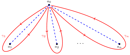
Figure 1. A possible visualization of the red fundamental loops $\gamma_{i}$.

The monodromy matrix at the singular point $a_{i}$ is defined as

$$G_{i}:=\chi([\gamma_{i}]),\ \ \ i=1,\ldots,n,$$

and we record the cyclic constraint $G_{1}\cdot\ldots\cdot G_{n}=\mathbb{I}\in\textnormal{GL}(p,\mathbb{C})$. Observe that the image of $\pi_{1}(S,a_{0})$ under (3.2), the monodromy group of system (3.1), is generated by the matrices $\{G_{1},\ldots,G_{n}\}$.

We are left with two obvious ambiguities in our definitions: first, if we were to start from a different fundamental solution $\Psi^{\ast}(z)$ instead of $\Psi(z)$, then $\Psi^{\ast}(z)=\Psi(z)H$ for some $H\in\textnormal{GL}(p,\mathbb{C})$ and the associated monodromy matrices change accordingly,

$$G_{i}^{\ast}=H^{-1}G_{i}H,\ \ i=1,\ldots,n.$$ (3.3)

Second, the dependence of $\pi_{1}(S,a_{0})$ and thus $G_{i}=\chi([\gamma_{i}])$ on the base point $a_{0}$: given that $S$ is path connected we know that $\pi_{1}(S,a_{0})$ and $\pi_{1}(S,a_{0}^{\ast})$ are isomorphic for any two base points $a_{0},a_{0}^{\ast}$ different from $a_{1},\ldots,a_{n}$, thus under the representation (3.2) the associated monodromy matrices change also in the style of (3.3). Hence, summarizing the two ambiguities, the monodromy of (3.1) is defined up to conjugation equivalence and so an element of the space

$$\mathcal{M}:=\textnormal{Hom}\big{(}\pi_{1}(S,a_{0}),\textnormal{GL}(p,\mathbb{C})\big{)}\big{/}\textnormal{GL}(p,\mathbb{C}),$$

of conjugacy classes of representations of $\pi_{1}(S,a_{0})$. Alternatively, in the language of monodromy matrices, we have

$$\mathcal{M}\cong\big{\{}(G_{1},\ldots,G_{n}):\,G_{1}\cdot\ldots\cdot G_{n}=\mathbb{I}\big{\}}\big{/}\textnormal{GL}(p,\mathbb{C}).$$ (3.4)

One notion remains: we say system (3.1) is Fuchsian if all its singular points $\{a_{1},\ldots,a_{n}\}$ are first order poles of $A(z)$, i.e. without loss of generality (thanks to a fractional linear map) we have

$$A(z)=\sum_{i=1}^{n}\frac{B_{i}}{z-a_{i}},\ \ \ \ \ \ \ \ \ \ \ \ \mathop{\mathrm{res}}\limits_{z=\infty}A(z)=-\sum_{i=1}^{n}B_{i}=0.$$

Using the above terminology we are now able to rephrase RHP 2.1 in interpretation (3) as follows:

Riemann-Hilbert Problem 3.1 (The original RHP, case (3)).

Is the monodromy map $\mu:\mathcal{M}^{\ast}\rightarrow\mathcal{M}$ from the space

$$\mathcal{M}^{\ast}:=\left\{(B_{1},\ldots,B_{n}):\ \ B_{i}\in\mathbb{C}^{p\times p},\ \ \sum_{i=1}^{n}B_{i}=0\right\}\bigg{/}\textnormal{GL}(p,\mathbb{C})$$

of Fuchsian systems with fixed singularities $a_{1},\ldots,a_{n}$ into $\mathcal{M}$ surjective?

This problem concludes our content on the necessary background terminology of Hilbert’s $21$st problem. We will now review some of the mathematical works devoted to its solution and which were published between $1908$ and $1989$. These works introduced several key ideas and techniques that are nowadays used in the Riemann-Hilbert analysis of OPSFA-type problems.

4. Plemelj’s contributions

In 1908, Plemelj [P0] (upgraded to book form 55 years later in [Pl]) published a solution of RHP 3.1 that was widely accepted until the early 1980s. In his work, he reduced RHP 3.1 to a Hilbert boundary value problem in the theory of singular integral equations and the idea goes as follows: Join all singularities $a_{1},\ldots,a_{n}\in\mathbb{C}$ by a simple closed oriented contour $\Gamma$ as indicated in Figure 2 below.

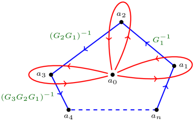
Figure 2. The oriented contour $\Gamma$ in blue together with the aformentioned red fundamental loops $\gamma_{i}$. Some values of $G(z)$ are indicated in green.

Now define the piecewise constant, matrix-valued and invertible function

$$G(z):=(G_{i}G_{i-1}\cdot\ldots\cdot G_{1})^{-1},\ \ \ z\in[a_{i},a_{i+1}),\ \ \ \ i=1,\ldots,n;\ \ \ \ a_{n+1}:=a_{1},$$

which, thanks to the cyclic constraint (3.4), satisfies $G(z)=\mathbb{I}$ for $z\in[a_{n},a_{1})$. With $\Omega^{+}$ denoting the region in $\mathbb{C}$ bounded by $\Gamma$ and $\Omega^{-}$ the complement of the closure $\overline{\Omega^{+}}$ in $\mathbb{CP}^{1}$, we then consider the following boundary value problem:

Hilbert Boundary Value Problem 4.1 ([P0, page $213,214,229$]).

Find all vector-valued functions $X=X(z)\in\mathbb{C}^{1\times p}$ such that

1. $X(z)$ is analytic in $\Omega^{\pm}\setminus\{\infty\}$ and extends continuously from either side to the punctured contour $\Gamma\setminus\{a_{1},\ldots,a_{n}\}$.

2. On the open segments $(a_{i},a_{i+1}),i=1,\ldots,n$ the pointwise limits

   $$X_{\pm}(z):=\lim_{\begin{subarray}{c}w\rightarrow z\\ w\in\Omega^{\pm}\end{subarray}}X(w)$$

   satisfy the boundary condition $X_{+}(z)=X_{-}(z)G(z)$, compare Figure 3 below.

   

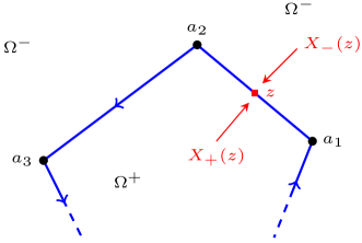
   Figure 3. The pointwise limits $X_{\pm}(z)$ at some $z\in(a_{i},a_{i+1}),i=1,\ldots,n$ in red.

3. $X(z)$ is of finite degree at $z=\infty$, that is

   $$X(z)=\gamma(z)+\mathcal{O}\big{(}z^{-1}\big{)},\ \ \ \ \ |z|\rightarrow\infty,$$ (4.1)

   with some vector-valued polynomial $\gamma\in\mathbb{C}^{1\times p}[z]$. Moreover, in a small neighborhood of $a_{i}$,

   $$\big{\|}X(z)\big{\|}\leq\frac{C}{|z-a_{i}|^{\alpha}},\ \ \ \ \ 0\leq\alpha<1,\ \ \ C>0.$$

With Problem 4.1 as starting point, Plemelj first proved its solvability through an application of Fredholm’s theory of integral equations, cf. [Fre, P1], at the time a novel analytic tool. We will lay out some of his steps below subject to the following two temporary assumptions:

Assumption 4.2.

We seek solutions of Problem 4.1 which extend Hölder continuously from either side up to the punctured contour $\Gamma\setminus\{a_{1},\ldots,a_{n}\}$.

Assumption 4.3.

The invertible jump matrix $G(z),z\in\Gamma$ in condition $(2)$ of Problem 4.1 is Hölder continuous on all of $\Gamma$ and not just on each open segment $(a_{i},a_{i+1})$ separately. In turn, the blow up constraint near $z=a_{i}$ in Problem 4.1 $(3)$ becomes unnecessary.

Contingent on these assumptions, Problem 4.1 is equivalent to the problem of finding all Hölder continuous functions $X_{-}(z)\in\mathbb{C}^{1\times p}$ defined for $z\in\Gamma$ such that

$$\forall\,z\in\Omega^{-}:\ 0=\frac{1}{2\pi\mathrm{i}}\int_{\Gamma}\frac{X_{-}(\lambda)G(\lambda)}{\lambda-z}\,{\mathrm{d}}\lambda;\ \ \ \ \ \textnormal{and}\ \ \ \ \ \forall\,z\in\Omega^{+}:\ 0=-\frac{1}{2\pi\mathrm{i}}\int_{\Gamma}\frac{X_{-}(\lambda)}{\lambda-z}\,{\mathrm{d}}\lambda+\gamma(z).$$ (4.2)

Indeed, by Cauchy’s theorem and Plemelj’s own $1908$ formulæ [P2] (the Plemelj-Sokhotski formulæ  which Plemelj rediscovered) the first constraint in (4.2) holds precisely when $X_{-}(z)G(z),z\in\Gamma$ is the boundary value of a function $X(z)\in\mathbb{C}^{1\times p}$ which is analytic in $\Omega^{+}$ and Hölder continuous on $\Omega^{+}\cup\Gamma$. Likewise the second constraint in (4.2) holds if and only if $X_{-}(z),z\in\Gamma$ is the boundary value of some $X(z)\in\mathbb{C}^{1\times p}$, analytic in $\Omega^{-}\setminus\{\infty\}$, Hölder continuous on $(\Omega^{-}\setminus\{\infty\})\cup\Gamma$ and of finite degree at $z=\infty$, in the sense of (4.1). Next, Plemelj noticed that both constraints in (4.2) are equivalent (again by Cauchy’s theorem and the Plemelj-Sokhotski formulæ) to the principal value integral equations,

$$X_{-}(z)=-\frac{1}{\pi\mathrm{i}}\,\textnormal{pv}\int_{\Gamma}\frac{X_{-}(\lambda)}{\lambda-z}\,{\mathrm{d}}\lambda+2\gamma(z),\ \ \ X_{-}(z)G(z)=\frac{1}{\pi\mathrm{i}}\,\textnormal{pv}\int_{\Gamma}\frac{X_{-}(\lambda)G(\lambda)}{\lambda-z}\,{\mathrm{d}}\lambda,\ \ \ \ z\in\Gamma,$$ (4.3)

and from these one obtains in turn the quasi-regular integral equation

$$X_{-}(z)-\frac{1}{\pi\mathrm{i}}\,\textnormal{pv}\int_{\Gamma}X_{-}(\lambda)\frac{K(z,\lambda)}{\lambda-z}\,{\mathrm{d}}\lambda=\gamma(z),\ \ \ z\in\Gamma,$$ (4.4)

with the Hölder continuous matrix-valued kernel function

$$K(z,\lambda):=\frac{1}{2}\big{(}G(\lambda)-G(z)\big{)}(G(z))^{-1},\ \ \ (z,\lambda)\in\Gamma\times\Gamma.$$

Remark 4.4.

In more abstract and general terms, the left hand side in (4.4) defines a singular Fredholm operator

$$(K\phi)(z):=\phi(z)-\frac{1}{\pi\mathrm{i}}\,\textnormal{pv}\int_{\Gamma}\phi(\lambda)\frac{K(z,\lambda)}{\lambda-z}\,{\mathrm{d}}\lambda,\ \ \ z\in\Gamma,$$

of index zero which acts on Hölder continuous functions defined on $\Gamma$, cf. [M, $\S 45$], and we assume that $K(z,\lambda)$ satisfies a Hölder condition on $\Gamma$ in both variables. Plemelj did not work with such singular Fredholm equations in [P0] since he managed to transform the piecewise constant jumps in Problem 4.1 to differentiable ones. In turn, his [P0, $(4)$] is an ordinary Fredholm equation of the second kind which can be studied by Fredholm’s $1903$ theory. We will discuss a more generally applicable reduction of piecewise Hölder continuous jumps to Hölder continuous ones and en route lift Assumption 4.3 on $G(z)$. In fact, the general theory of singular Fredholm integral equations of the type (4.4) was systematically developed some $30$ years after Plemelj’s paper with prominent contributions by Giraud [Gi], Muskhelishvili-Vekua [MV] and Gakhov [Ga2].

We now make (4.4) the starting point for the solvability analysis of Problem 4.1. Precisely, given that any continuous solution $X_{-}(z),z\in\Gamma$ of (4.4) will be automatically Hölder continuous as a consequence of Assumption 4.3, we answer the following two questions:

1. Under which conditions is (4.4) solvable in the space of continuous functions on $\Gamma$?

2. Does each continuous solution of (4.4) yield a solution of Problem 4.1?

Regarding Q2, we recall that every continuous solution $X_{-}(z),z\in\Gamma$ of (4.4) will produce a solution of Problem 4.1 with Assumption 4.3 in place if and only if $X_{-}(z),z\in\Gamma$ solves both equations in (4.3). Now rephrase (4.3) in terms of the function

$$\widehat{X}(z):=\begin{cases}\displaystyle\frac{1}{2\pi\mathrm{i}}\int_{\Gamma}\frac{X_{-}(\lambda)}{\lambda-z}\,{\mathrm{d}}\lambda-\gamma(z),&z\in\Omega^{+}\vskip 12.0pt plus 4.0pt minus 4.0pt\\ \displaystyle\frac{1}{2\pi\mathrm{i}}\int_{\Gamma}\frac{X_{-}(\lambda)G(\lambda)}{\lambda-z}\,{\mathrm{d}}\lambda,&z\in\Omega^{-}\end{cases},$$ (4.5)

which is analytic on $\Omega^{\pm}$, Hölder continuous on $\Omega^{\pm}\cup\Gamma$ and vanishes at $z=\infty$. In fact,

$$\eqref{e:6}\ \textnormal{holds}\ \ \ \Leftrightarrow\ \ \ \ \widehat{X}_{+}(z)=0=\widehat{X}_{-}(z),\ \ z\in\Gamma\ \ \ \Leftrightarrow\ \ \ \ \widehat{X}(z)\equiv 0\ \ \textnormal{in}\ \mathbb{C}$$ (4.6)

Furthermore, our central integral equation (4.4) is equivalent to the jump condition

$$\widehat{X}_{+}(z)=\widehat{X}_{-}(z)(G(z))^{-1},\ \ z\in\Gamma,$$

which motivates the introduction of the below, after Plemelj the accompanying, Hilbert boundary value problem:

Hilbert Boundary Value Problem 4.5 ([P0, page $215$]).

Find all vector-valued functions $\widehat{X}=\widehat{X}(z)\in\mathbb{C}^{p}$ such that

1. $\widehat{X}(z)$ is analytic in $\Omega^{\pm}$ and extends Hölder continuously from either side up to $\Gamma$.

2. The pointwise limits

   $$\widehat{X}_{\pm}(z):=\lim_{\begin{subarray}{c}w\rightarrow z\\ w\in\Omega^{\pm}\end{subarray}}\widehat{X}(w),\ \ \ z\in\Gamma,$$

   satisfy the boundary condition $\widehat{X}_{+}(z)=\widehat{X}_{-}(z)(G(z))^{-1},z\in\Gamma$.

3. $\widehat{X}(z)$ vanishes at $z=\infty$, that is

   $$\widehat{X}(z)=\mathcal{O}\big{(}z^{-1}\big{)},\ \ \ \ \ |z|\rightarrow\infty.$$

The special homogeneous problem 4.5 is useful since it allows us to summarize our previous chain (4.6) as the following exclusive alternative: let $X_{-}(\lambda),\lambda\in\Gamma$ be a continuous solution of (4.4),

$\diamond$ If $\widehat{X}(z)$ defined in terms of said $X_{-}(\lambda),\lambda\in\Gamma$ in (4.5) is identically zero, then $X_{-}(\lambda)$ solves (4.3) and thus produces a solution of the initial Problem 4.1.

$\diamond$ If $\widehat{X}(z)$ defined in terms of said $X_{-}(\lambda),\lambda\in\Gamma$ in (4.5) is not identically zero, then $\widehat{X}(z)$ is a non-trivial solution of the accompanying Problem 4.5.

Most importantly we can now formulate Plemelj’s first criterion as response to Q2 above:

Lemma 4.6 ([P0, page $215$]).

If the accompanying Problem 4.5 has no non-trivial solutions, then every continuous solution $X_{-}(z),z\in\Gamma$ of (4.4) yields a solution of Problem 4.1.

Evidently, Lemma 4.6 does not guarantee solvability of (4.4). Indeed, in order to answer Q1, Plemelj used Fredholm’s theory of integral equations. First, consider two additional homogeneous Hilbert boundary value problems: the associated Hilbert boundary value problem which consists in finding $Y=Y(z)\in\mathbb{C}^{1\times p}$ that is analytic in $\Omega^{\pm}$, extends Hölder continuously up to $\Gamma$, vanishes at infinity and instead of the jump condition in Problem 4.5 satisfies

$$Y_{+}(z)=Y_{-}(z)\big{(}G^{\top}(z)\big{)}^{-1},\ \ z\in\Gamma,$$ (4.7)

with the matrix transpose $G^{\top}(z)$ of $G(z)$. Moreover, the problem which accompanies the associated problem (4.7) and which seeks $\widehat{Y}=\widehat{Y}(z)\in\mathbb{C}^{1\times p}$ as in Problem 4.5 but with jump constraint

$$\widehat{Y}_{+}(z)=\widehat{Y}_{-}(z)G^{\top}(z),\ \ z\in\Gamma.$$ (4.8)

Repeating the logic that took us from Problem 4.1 (with Assumptions 4.2 and 4.3) to equation (4.4) we easily see that (4.8) leads to the integral equation

$$\widehat{Y}_{+}(z)+\frac{1}{\pi\mathrm{i}}\,\textnormal{pv}\int_{\Gamma}\widehat{Y}_{+}(\lambda)\frac{K^{\top}(\lambda,z)}{\lambda-z}\,{\mathrm{d}}\lambda=0,\ \ z\in\Gamma,$$ (4.9)

and which is the adjoint equation of (4.4). We can now derive Plemelj’s second criterion:

Lemma 4.7 ([P0, page $217,218$]).

If the associated problem (4.7) has no non-trivial solutions, then (4.4) is solvable in the space of continuous functions on $\Gamma$ for any given $\gamma\in\mathbb{C}^{1\times p}[z]$.

Proof.

Problem (4.8) accompanies the associated problem (4.7), or equivalently, (4.7) is the accompanying problem of (4.8) (as we invert the jump matrix and homogenize at infinity in the accompanying problems). But by assumption, (4.7) has no non-trivial solutions, so by Lemma 4.6 every continuous solution $\widehat{Y}_{+}(z),z\in\Gamma$ of the adjoint equation (4.9) yields a solution of the Hilbert boundary value problem (4.8). Let $\widehat{Y}_{+}(z),z\in\Gamma$ denote such a non-trivial continuous solution of (4.9), so $\widehat{Y}_{+}(z),z\in\Gamma$ is the boundary value of some analytic function $\widehat{Y}(z),z\in\Omega^{+}$. However, by [N, $(7)$], the inhomogeneous equation (4.4) is continuously solvable if and only if

$$\int_{\Gamma}\gamma(z)\widehat{Y}_{+}^{\top}(z)\,{\mathrm{d}}z=0,$$

and which is guaranteed by our last conclusion and the fact that $\gamma\in\mathbb{C}^{1\times p}[z]$ (any entire $\gamma(z)$ would do). This concludes the proof of the Lemma. ∎

To summarize, Lemma 4.6 and 4.7 guarantee solvability of our initial Problem 4.1 (with Assumption 4.3 in place, but no longer Assumption 4.2), provided the accompanying Problem 4.5 and the associated problem (4.7) are only trivially solvable. Although these two conditions seem peculiar they are in fact easily verifiable from our assumption that $\gamma(z)$ is polynomial and thus our solutions of Problem 4.1 meromorphic at $z=\infty$. Indeed, we first recall, cf. [N, $\S 2$], that the homogeneous version of (4.4) (or any of the other homogeneous equations in this section) has finitely many, say $s\in\mathbb{Z}_{\geq 1}$, linearly independent continuous solutions. Then

Proposition 4.8 ([P0, page $219$]).

Any solution $X(z)$ of Problem 4.1 (with Assumption 4.3) has a zero of order at most $s\in\mathbb{Z}_{\geq 1}$ at $z=\infty$.

Proof.

If $X(z)$ has a zero of order $k\in\mathbb{Z}_{\geq 1}$ at $z=\infty$, then

$$X(z),\,zX(z),\,z^{2}X(z),\,\ldots,\,z^{k-1}X(z)$$

all solve the homogeneous version of Problem 4.5 (with Assumption 4.3) and thus $X_{-}(z),zX_{-}(z)$, $z^{2}X_{-}(z),\ldots$, $z^{k-1}X_{-}(z),z\in\Gamma$ all solve (4.4) with $\gamma\equiv 0$. Since these solutions are linearly independent we must have $k\leq s$ by our previous discussion. ∎

So we can always find an integer $r\in\mathbb{Z}_{\geq 0}$ such that neither the accompanying problem 4.1 nor the associated problem (4.7) admit solutions with a zero of order greater than $r$ at $z=\infty$. Hence, if $X(z)$ solves Problem 4.1 where $\gamma\in\mathbb{C}^{1\times p}[z]$ satisfies $\textnormal{deg}(\gamma)\leq r$, then

$$X^{\circ}(z):=\begin{cases}\displaystyle X(z),&z\in\Omega^{+}\vskip 3.0pt plus 1.0pt minus 1.0pt\\ \displaystyle\frac{X(z)}{(z-z_{0})^{r}},&z\in\Omega^{-}\end{cases}\ \ \ \ \ \ \ \ \textnormal{for some arbitrary}\ \ z_{0}\in\Omega^{+},$$ (4.10)

solves Problem 4.1 with jump matrix $G^{\circ}(z):=(z-z_{0})^{r}G(z)$ and is bounded at $z=\infty$. Most importantly, the central assumptions in Lemma 4.6 and 4.7 for the accompanying and associated problem of the $X^{\circ}$-Hilbert boundary value (which is Problem 4.1 with $X^{\circ}(z)=\mathcal{O}(1)$ at $z=\infty$ and Hölder continuous jumps on all of $\Gamma$) are satisfied:

1. The accompanying problem has jump $\widehat{X}_{+}^{\circ}(z)=\widehat{X}^{\circ}_{-}(z)(z-z_{0})^{-r}(G(z))^{-1}$, $z\in\Gamma$, so if this problem has a non-trivial solution (that vanishes at infinity) then

   $$\widehat{X}(z):=\begin{cases}\widehat{X}^{\circ}(z),&z\in\Omega^{+}\vskip 3.0pt plus 1.0pt minus 1.0pt\\ (z-z_{0})^{-r}\widehat{X}^{\circ}(z),&z\in\Omega^{-}\end{cases}$$

   solves Problem 4.5 and has a zero of order greater than $r$ at $z=\infty$, contradicting our initial choice for $r$.

2. The associated problem has jump $Y^{\circ}_{+}(z)=Y^{\circ}_{-}(z)(z-z_{0})^{-r}(G^{\top}(z))^{-1}$, $z\in\Gamma$, so if this problem has a non-trivial solution (that vanishes at infinity) then

   $$Y(z):=\begin{cases}Y^{\circ}(z),&z\in\Omega^{+}\\ (z-z_{0})^{-r}\,Y^{\circ}(z),&z\in\Omega^{-}\end{cases}$$

   solves the associated problem (4.7) and vanishes to order greater than $r$ at $z=\infty$. Again a contradiction to our choice of $r$.

The $X^{\circ}$-Hilbert boundary value problem is thus solvable by Lemma 4.6 and 4.7 and by reversing (4.10) we arrive at

Theorem 4.9 ([P0, page $222,223$]).

There exists $r\in\mathbb{Z}_{\geq 1}$ such that Problem 4.1 (with Assumption 4.3) is solvable for all $\gamma\in\mathbb{C}^{1\times p}[z]$ with $\textnormal{deg}(\gamma)\leq r$. Moreover, every solution of said problem is of the form

$$X(z)=\sum_{i=1}^{p}\gamma_{i}X_{i}(z)+\sum_{i=p+1}^{m}\gamma_{i}X_{i}(z),\ \ z\in\mathbb{C}\setminus\Gamma,$$ (4.11)

with some constants $\gamma_{1},\ldots,\gamma_{m}\in\mathbb{C}$ and where $\{X_{i}(z)\}_{j=1}^{m}$ are linearly independent particular solutions of Problem 4.1 with

$$\lim_{|z|\rightarrow\infty}z^{-r}X^{ij}(z)=\delta_{ij},\ \ \ \ i,j=1,\ldots,p;\ \ \ \ \ \ \ \ \ \ \ \ X_{i}(z)=\big{[}X^{ij}(z)\big{]}_{j=1}^{p}\in\mathbb{C}^{1\times p},$$

and $\{X_{i}(z)\}_{i=p+1}^{m}$ (if there are any) have degree strictly less than $r$ at $z=\infty$.

Proof.

Clearly, if $\{X_{i}\}_{j=1}^{m}$ are any particular solutions of the jump condition in Problem 4.1, then any polynomial linear combination of them will also solve the same jump constraint. Thus, choosing $r\in\mathbb{Z}_{\geq 1}$ sufficiently large as indicated in our previous discussion we can always ensure that Problem 4.1 is solvable for the collection of constant polynomials $\gamma_{i}(z)=[\delta_{ij}]_{j=1}^{p}$ with $i=1,\ldots,p$. Reversing subsequently (4.10) and taking an arbitrary combination of the so obtained solutions yields the first half in (4.11) with the indicated asymptotic behavior at $z=\infty$. The second sum in (4.11) stems from the complete system of linearly independent solutions of the homogeneous version of Problem 4.1, modulo the inversion of (4.10). ∎

Although Theorem 4.9 solves Problem 4.1, the implicit dependence of (4.11) on $r\in\mathbb{Z}_{\geq 1}$ is a drawback, in particular since $r$ affects $X^{\circ}(z)$ through (4.10) and it affects the parameter $m$. In order to bypass these deficiencies Plemelj managed then to construct a fundamental system $\{F_{i}\}_{i=1}^{p}\subset\mathbb{C}^{1\times p}$ of solutions to Problem 4.1 such that every solution of the same problem is a polynomial linear combination of the form

$$X(z)=\sum_{i=1}^{p}q_{i}(z)F_{i}(z),\ \ z\in\mathbb{C}\setminus\Gamma;\ \ \ \ \ \ q_{i}\in\mathbb{C}[z].$$

In order to present his argument, we first note that the system $\{X_{i}\}_{i=1}^{p}$ in (4.11) is linearly independent over $\mathbb{C}[z]$ because of its asymptotic normalization. With $r\in\mathbb{Z}_{\geq 1}$ as stated in Theorem 4.9, we then observe that among all solutions of the form (4.11) some have the lowest degree at $z=\infty$ since a solution of Problem 4.1 cannot vanish to all orders at $z=\infty$. Let $F_{1}(z)$ denote one of the solutions of lowest degree $-\nu_{1}\in\mathbb{Z}$ at $z=\infty$ and $F_{2}(z)$ one of the solutions of Problem 4.1 of lowest degree $-\nu_{2}\geq-\nu_{1}$ at $z=\infty$ such that $F_{2}\notin\textnormal{span}\{F_{1}\}$. Next, we let $F_{3}(z)$ denote one of the solutions of Problem 4.1 of lowest degree $-\nu_{3}\geq-\nu_{2}$ at $z=\infty$ such that $F_{3}\notin\textnormal{span}\{F_{1},F_{2}\}$ and note that this process may be continued until we reach $F_{p}\notin\textnormal{span}\{F_{1},\ldots,F_{p-1}\}$ of lowest degree $-\nu_{p}\geq-\nu_{p-1}$ at $z=\infty$. Indeed, if $F_{1}(z),\ldots,F_{k}(z)$ with $k<p$ have been constructed in this fashion then we can find yet another solution of Problem 4.1 not contained in $\textnormal{span}\{F_{1},\ldots,F_{k}\}$. For otherwise, the particular solutions $\{X_{i}\}_{i=1}^{p}$ in (4.11) would be contained in $\textnormal{span}\{F_{1},\ldots,F_{k}\}$ and thus be linearly dependent over $\mathbb{C}[z]$, contradicting our previous discussion. In summary, the above procedure leads to $p$ fundamental solutions

$$F_{1}(z),F_{2}(z),\ldots,F_{p}(z),$$ (4.12)

of Problem 4.1 with lowest degrees $-\nu_{1},-\nu_{2},\ldots,-\nu_{p}$ at $z=\infty$ where $\nu_{1}\geq\nu_{2}\geq\ldots\geq\nu_{p}$ and $F_{k}\notin\textnormal{span}\{F_{1},\ldots,F_{k-1}\}$ for $k=2,\ldots,p$. The central properties of the so constructed fundamental system (4.12) are summarized below.

Theorem 4.10 ([P0, page $227$]).

There exists $r\in\mathbb{Z}_{\geq 1}$ such that Problem 4.1 (with Assumption 4.3) is solvable for all $\gamma\in\mathbb{C}^{1\times p}[z]$ with $\textnormal{deg}(\gamma)\leq r$. Moreover, every solution of said problem is of the form

$$X(z)=\sum_{i=1}^{p}q_{i}(z)F_{i}(z),\ \ \ z\in\mathbb{C}\setminus\Gamma,$$ (4.13)

where $\{F_{i}\}_{j=1}^{p}$ is a fundamental system of solutions, $q_{i}\in\mathbb{C}[z]$ and the corresponding fundamental matrix

$$\Phi(z):=\big{[}F^{ij}(z)\big{]}_{i,j=1}^{p},\ \ \ \ \ F_{i}(z)=\big{[}F^{ij}(z)\big{]}_{j=1}^{p}\in\mathbb{C}^{1\times p},\ \ \ z\in\mathbb{C}\setminus\Gamma$$

satisfies

• $\det\Phi(z)\neq 0$ for all $z\in\mathbb{C}$ including $z\in\Gamma$ with the appropriate limiting values $\Phi_{\pm}(z)$.

• There exists a diagonal matrix $\Lambda\in\mathbb{Z}^{p\times p}$ such that $z^{\Lambda}\Phi(z)$ is invertible at $z=\infty$.

Proof.

The first statement of the theorem was already established in Theorem 4.9 and (4.13) follows from (i) since by construction of the fundamental matrix, $G(z)=(\Phi_{-}(z))^{-1}\Phi_{+}(z),z\in\Gamma$ and thus for any solution $X(z)$ of Problem 4.1 (with Assumption 4.3),

$$X_{+}(z)(\Phi_{+}(z))^{-1}=X_{-}(z)(\Phi_{-}(z))^{-1},\ \ z\in\Gamma,$$

i.e. $X(z)(\Phi(z))^{-1}$ is an entire function. Hence, by condition (3) in Problem 4.1 we find that $X(z)(\Phi(z))^{-1}\in\mathbb{C}^{1\times p}[z]$, so (4.13) follows and conversely it is clear that the right hand side in (4.13) solves the Hilbert boundary value problem 4.1 for any $q_{i}\in\mathbb{C}[z]$. In order to establish (i) we first note that if $X(z)$ is any solution of Problem 4.1 of degree strictly less than $-\nu_{k}\in\mathbb{Z}$ at $z=\infty$ where $k\in\{2,\ldots,p\}$, then necessarily

$$X(z)=\sum_{i=1}^{k-1}r_{i}(z)F_{i}(z)\ \ \ \textnormal{for some}\ r_{i}\in\mathbb{C}[z].$$ (4.14)

For if such $X$, i.e. of degree strictly less than $-\nu_{k}$ at $z=\infty$, were not contained in $\textnormal{span}\{F_{1},\ldots,F_{k-1}\}$, then our previous selection process of the subsequent $F_{k}\notin\textnormal{span}\{F_{1},\ldots,F_{k-1}\}$ with lowest degree $-\nu_{k}\geq-\nu_{k-1}$ would fail. Returning to (i) we now show that the expression

$$F(z):=\sum_{i=1}^{p}a_{i}F_{i}(z),\ \ \ \ z\in\mathbb{C}\setminus\Gamma,$$ (4.15)

with $a_{i}\in\mathbb{C}$ not all zero, does not vanish at any point $z\in\mathbb{C}$: if $F(z_{0})=0$ for some $z_{0}\notin\Gamma$, then

$$(z-z_{0})X(z)=\sum_{i=1}^{p}a_{i}F_{i}(z),\ \ \ \ z\in\mathbb{C}\setminus\Gamma$$

where $X(z)$ solves Problem 4.1. If $a_{k}$ denotes the last of the coefficients $a_{1},\ldots,a_{p}$ which is non-zero, then the degree of $X(z)$ at $z=\infty$ is strictly less than $-\nu_{k}$, so (4.14) must hold for the same $X(z)$, i.e. we would have

$$(z-z_{0})\sum_{i=1}^{k-1}r_{i}(z)F_{i}(z)=\sum_{i=1}^{k}a_{i}F_{i}(z).$$

But this is a contradiction to the requirement $F_{k}\notin\textnormal{span}\{F_{1},\ldots,F_{k-1}\}$ and thus $F(z)\neq 0$ for all $z\in\mathbb{C}\setminus\Gamma$. If on the other hand $F(z_{0})=0$ for some $z_{0}\in\Gamma$, i.e. either $F_{+}(z_{0})=0$ or equivalently $F_{-}(z_{0})=F_{+}(z_{0})(G(z_{0}))^{-1}=0$, then define

$$X(z):=\frac{F(z)}{z-z_{0}},\ \ \ z\in\mathbb{C}\setminus\Gamma.$$

This $\mathbb{C}^{1\times p}$-valued function is analytic in $\Omega^{\pm}\setminus\{\infty\}$, of finite degree at $z=\infty$ and extends Hölder continuously from either side to the punctured contour $\Gamma\setminus\{z_{0}\}$. Thus the above $X(z)$ solves the singular integral equation (4.4) for all $z\in\Gamma\setminus\{z_{0}\}$ and since $F_{\pm}(z),z\in\Gamma$ are Hölder continuous with $F_{\pm}(z_{0})=0$ we conclude that $X_{-}(z),z\in\Gamma$ as well as $X_{+}(z)=X_{-}(z)G(z),z\in\Gamma$ are Hölder continuous on all of $\Gamma$. At this point we simply repeat the previous logic for $z_{0}\notin\Gamma$ and conclude $F(z)\neq 0$ for all $z\in\Gamma$. All together, (4.15) does not vanish for any $z\in\mathbb{C}$ (choosing $F_{\pm}(z)$ for $z\in\Gamma$) and thus $\det\Phi(z)\neq 0$ for all $z\in\mathbb{C}$, as claimed. We are left with (ii) and thus the point $z=\infty$ at which $\det\Phi(z)$ might have a pole or may remain finite. However, if $-\nu_{i}\in\mathbb{Z}$ denotes the degree of $F_{i}(z)$ at $z=\infty$, then

$$\det\big{[}z^{\nu_{i}}F^{ij}(z)\big{]}_{i,j=1}^{p}$$

is certainly finite at $z=\infty$. If it were zero, then we could find $a_{1},\ldots,a_{p}\in\mathbb{C}$ not all zero such that

$$a_{1}z^{\nu_{1}}F_{1}(z)+a_{2}z^{\nu_{2}}F_{2}(z)+\ldots+a_{p}z^{\nu_{p}}F_{p}(z)=\mathcal{O}\big{(}z^{-1}\big{)},\ \ \ \ \textnormal{as}\ \ \ z\rightarrow\infty.$$

With $a_{k}$ denoting the last of the coefficients $a_{1},\ldots,a_{p}$ which is non-zero we then have

$$X(z):=a_{1}z^{\nu_{1}-\nu_{k}}F_{1}(z)+a_{2}z^{\nu_{2}-\nu_{k}}F_{2}(z)+\ldots+a_{k}F_{k}(z)=\mathcal{O}\big{(}z^{-1-\nu_{k}}\big{)},\ \ \ z\rightarrow\infty,$$

i.e. the degree of $X(z)$ at $z=\infty$ is strictly less than $-\nu_{k}$. But then necessarily (compare above)

$$X(z)=\sum_{i=1}^{k-1}r_{i}(z)F_{i}(z)\ \ \ \ \ \ \textnormal{for some}\ \ r_{i}\in\mathbb{C}[z],$$

and in turn $F_{k}\in\textnormal{span}\{F_{1},\ldots,F_{k-1}\}$, a contradiction. All together,

$$z^{\Lambda}\Phi(z)\ \ \ \ \ \textnormal{with}\ \ \Lambda:=\textnormal{diag}[\nu_{1},\ldots,\nu_{p}]\in\mathbb{Z}^{p\times p}$$

is invertible at $z=\infty$. This concludes the proof of the theorem. ∎

Plemelj’s central Theorem 4.10 will be the key to solve RHP 2.1 in interpretation (2), provided we can dispose of Assumption 4.3. In [P0, page $229-236$] this was achieved by relying on the piecewise constant nature of $G(z)$ in Problem 4.1. Here, we shall outline a procedure of Vekua [V, Chapter $2$] which is more widely applicable and which employs multi-valued analytic functions defined in cut planes, equivalently discontinuous single-valued functions. First, we denote with

$$G(a_{j}\mp 0),\ \ j=1,\ldots,n$$

the left, resp. right limits at the point $a_{j}\in\Gamma$ as we approach $a_{j}$ along $(a_{j-1},a_{j})$, resp. $(a_{j},a_{j+1})$ on $\Gamma$, compare Figure 2. These limits exist by our definition of $G(z)$ and we call $a_{\sigma}\in\{a_{1},\ldots,a_{n}\}$ with $G(a_{\sigma}-0)\neq G(a_{\sigma}+0)$ a point of discontinuity. Second, we use the eigenvalues $\lambda_{1}^{\sigma},\ldots,\lambda_{p}^{\sigma}$ of the non-singular matrix $G(a_{\sigma}-0)(G(a_{\sigma}+0))^{-1}$ at a point of discontinuity $a_{\sigma}$ written as

$$j=1,\ldots,p:\ \ \ \ \lambda_{j}^{\sigma}=\mathrm{e}^{2\pi\mathrm{i}\gamma_{j}^{\sigma}},\ \ \ \ \ \ \ \ \ \ \ \ \gamma_{j}^{\sigma}\in\mathbb{C}:\ -\frac{1}{2}<\textnormal{Re}\,\gamma_{j}^{\sigma}\leq\frac{1}{2}.$$

Third, we fix $z_{0}\in\Omega^{+}$ and let $L^{\sigma}$ denote the straight line connecting $z_{0}$ with a point of discontinuity $a_{\sigma}$ and extending to $z=\infty$. With this convention any branch of

$$d_{j}^{\,\sigma}(z):=(z-z_{0})^{\gamma_{j}^{\sigma}},\ \ \ z\in\mathbb{C}\setminus L^{\sigma},\ \ \ \ j=1,\ldots,p,$$

is single-valued and we have

$$\forall\,w\in\Gamma\setminus\{a_{\sigma}\}:\ \ \lim_{\begin{subarray}{c}z\rightarrow w\\ z\in\Omega^{+}\end{subarray}}d_{j}^{\,\sigma}(z)=\lim_{\begin{subarray}{c}z\rightarrow w\\ z\in\Omega^{-}\end{subarray}}d_{j}^{\,\sigma}(z),\ \ \ \ \ \ \ \ \textnormal{as well as}\ \ \ \ \ \ \ \ \frac{d_{j}^{\,\sigma}(a_{\sigma}-0)}{d_{j}^{\,\sigma}(a_{\sigma}+0)}=\mathrm{e}^{2\pi\mathrm{i}\gamma_{j}^{\sigma}}.$$

We also need an arbitrary branch of the function $(z-a_{\sigma})^{\gamma_{j}^{\sigma}}$ defined in $\mathbb{C}$ with a cut along $[a_{\sigma},\infty)\subset L^{\sigma}$ and the function $(\frac{z-a_{\sigma}}{z-z_{0}})^{\gamma_{j}^{\sigma}}$ uniquely defined in $\mathbb{C}$ with a cut on $[z_{0},a_{\sigma}]\subset L^{\sigma}$ such that $(\frac{z-a_{\sigma}}{z-z_{0}})^{\gamma_{j}^{\sigma}}\rightarrow 1$ as $z\rightarrow\infty$. We now come to the heart of Vekua’s method: define the diagonal matrices

$$A_{\sigma}(z):=\bigoplus_{j=1}^{p}\left(\frac{z-a_{\sigma}}{z-z_{0}}\right)^{\gamma_{j}^{\sigma}},\ \ \ \ B_{\sigma}(z):=\bigoplus_{j=1}^{p}(z-a_{\sigma})^{\gamma_{j}^{\sigma}},\ \ \ \ C_{\sigma}(z):=\bigoplus_{j=1}^{p}d_{j}^{\,\sigma}(z),$$

and note that $A_{\sigma}(z)$ is analytic in $\Omega^{-}$ whereas any branch of $B_{\sigma}(z)$ is analytic in $\Omega^{+}$. But if $X(z)$ solves Problem 4.1 then

$$T(z):=X(z)\begin{cases}\displaystyle M_{\sigma}^{-1}(B_{\sigma}(z))^{-1},&z\in\Omega^{+}\vskip 3.0pt plus 1.0pt minus 1.0pt\\ \displaystyle N_{\sigma}^{-1}(A_{\sigma}(z))^{-1},&z\in\Omega^{-}\end{cases},$$ (4.16)

for properly chosen $M_{\sigma},N_{\sigma}\in\textnormal{GL}(p,\mathbb{C})$, will solve a modified Problem 4.1 with jump matrix which is Hölder continuous on the whole segment $(a_{\sigma-1},a_{\sigma+1})$ including the point $z=a_{\sigma}$. Once $a_{\sigma}$ has been removed in this fashion all remaining points of discontinuity can be treated similarly and we eventually arrive at a Hilbert boundary value problem that satisfies Assumption 4.3. So how do we choose $M_{\sigma}$ and $N_{\sigma}$? With (4.16) the jump condition on $\Gamma\setminus\{a_{1},\ldots,a_{n}\}$ in Problem 4.1 gets replaced by

$$T_{+}(z)= \,T_{-}(z)A_{\sigma}(z)N_{\sigma}\,G(z)M_{\sigma}^{-1}(B_{\sigma}(z))^{-1}$$

$$= \,T_{-}(z)\Big{(}\mathbb{I}+B_{\sigma}(z)\Big{[}(C_{\sigma}(z))^{-1}N_{\sigma}\,G(z)-M_{\sigma}\Big{]}M_{\sigma}^{-1}(B_{\sigma}(z))^{-1}\Big{)},$$

and this motivates the requirements

$$(C_{\sigma}(a_{\sigma}+0))^{-1}N_{\sigma}\,G(a_{\sigma}+0)=M_{\sigma}=(C_{\sigma}(a_{\sigma}-0))^{-1}N_{\sigma}\,G(a_{\sigma}-0)$$ (4.17)

to ensure that the jump for $T(z)$ is Hölder continuous on $(a_{\sigma-1},a_{\sigma+1})$. In fact, with (4.17) in place, the matrix $(C_{\sigma}(z))^{-1}N_{\sigma}\,G(z)-M_{\sigma}$ will be Lipschitz continuous on $(a_{\sigma-1},a_{\sigma+1})$, see [M, $\S 6$]. In order to make (4.17) more transparent, we use $C_{\sigma}(a_{\sigma}-0)(C_{\sigma}(a_{\sigma}+0))^{-1}=\bigoplus_{j=1}^{p}\lambda_{j}^{\sigma}$ and rewrite (4.17) as

$$N_{\sigma}\,G(a_{\sigma}-0)(G(a_{\sigma}+0))^{-1}N_{\sigma}^{-1}=\bigoplus_{j=1}^{p}\lambda_{j}^{\sigma},\ \ \ \ \ \ \ \ \ M_{\sigma}=\big{(}C_{\sigma}(a_{\sigma}+0)\big{)}^{-1}N_{\sigma}\,G(a_{\sigma}+0),$$

so $N_{\sigma}$ and $M_{\sigma}$ in (4.17) exist if $G(a_{\sigma}-0)(G(a_{\sigma}+0))^{-1}$ is diagonalizable. If this is not the case, then one has to properly modify $M_{\sigma},N_{\sigma}$ in (4.16) and work with the Jordan normal form of $G(a_{\sigma}-0)(G(a_{\sigma}+0))^{-1}$, see [V, page $87-93$] for details. Either way, a finite number of transformations of the type (4.16) lead to a Hilbert boundary value problem that is amenable to our previous analysis, i.e. a problem whose jump matrix is Hölder continuous along all of $\Gamma$ and which satisfies a normalization of the form (4.1).

At this point we can come full circle and return to the original RHP 2.1: each function of the fundamental system (4.12) can be analytically continued to any point in $\mathbb{C}\setminus\{a_{1},\ldots,a_{n}\}$ via any path that does not pass through any of the singularities. Concretely, if $\tau_{\gamma_{j}}$ denotes the operator of analytic continuation along the fundamental loop $\gamma_{j}$, compare Figure 2, then by Problem 4.1 condition (2), any fundamental matrix $\Phi(z)$ satisfies

$$\tau_{\gamma_{j}}(\Phi)(z)=\Phi(z)G_{j},\ \ \ \ j=1,\ldots,n.$$

But the same is also true for the matrix-valued function

$$\Psi(z):=(z-a_{1})^{\Lambda}\Phi(z),\ \ \ z\in\mathbb{CP}^{1}\setminus\Gamma$$ (4.18)

which, according to Theorem 4.10, is invertible and bounded at $z=\infty$. Using Liouville’s theorem and the piecewise constant, that is $z$-independent, form of $G(z)$ it now follows that the matrix

$$A(z):=\frac{{\mathrm{d}}\Psi}{{\mathrm{d}}z}(z)(\Psi(z))^{-1},\ \ \ \ z\in\mathbb{CP}^{1}\setminus\{a_{1},\ldots,a_{n}\}$$ (4.19)

is single-valued on $\mathbb{CP}^{1}$ and analytic everywhere expect at the singularities $a_{1},\ldots,a_{n}\in\mathbb{C}$. Moreover, using Problem 4.1, condition (3), (4.18) and our discussion on Vekua’s regularization, it is clear that $a_{1},\ldots,a_{n}$ are regular singular points of the system (4.19) in the following sense:

Definition 4.11.

Given a system (3.1) where $A(z)\in\mathbb{C}^{p\times p}$ is analytic in a punctured disk $\mathbb{D}_{r}(z_{0})\setminus\{z_{0}\}$ for some $r>0$, we say that $z_{0}$ is a regular singular point of (3.1) if any solution of the system has at most polynomial growth in a vicinity of $z_{0}$.

Since the system (4.19) also has the given monodromy $(G_{1},\ldots,G_{n})$, the above analysis solves RHP 2.1 in interpretation (2). Precisely

Theorem 4.12 (Plemelj, 1908).

Any matrix group with $n\in\mathbb{Z}_{\geq 1}$ generators $G_{1},\ldots,G_{n}\in\textnormal{GL}(p,\mathbb{C})$ satisfying the constraint $G_{1}\cdot\ldots\cdot G_{n}=\mathbb{I}$ can be realized as the monodromy group of a $p\times p$ linear system (3.1) on $\mathbb{CP}^{1}$ having only regular singularities.

Plemelj’s 1908 paper does not stop with Theorem 4.12: indeed, while all singularities in a Fuchsian system are always regular singular points (this is Sauvage’s 1886 theorem, cf. [CL, Theorem $2.1$] or [IY, Theorem $16.10$]), the converse statement is in general false. For instance, the non-Fuchsian system

$$\frac{{\mathrm{d}}\Psi}{{\mathrm{d}}z}=\left\{-\frac{3}{16z^{2}}\begin{bmatrix}0&0\\ 1&0\end{bmatrix}+\begin{bmatrix}0&1\\ 0&0\end{bmatrix}\right\}\Psi$$ (4.20)

has a fundamental solution of the form

$$\Psi(z)=\frac{1}{4}\begin{bmatrix}4z&4z\\ 1&3\end{bmatrix}z^{-\frac{1}{4}\bigl{[}\begin{smallmatrix}3&0\\ 0&1\end{smallmatrix}\bigr{]}},\ \ \ \ z\in\mathbb{C}\setminus(-\infty,0],$$

and thus $z=0$ is a regular singular point of system (4.20). Plemelj was aware of the distinction between regular singular and Fuchsian singular points, thus he applied a gauge procedure that took him from (4.19) to another system with equal monodromy and same singular points. The transformed system is Fuchsian for all except perhaps one singular point. This part in Plemelj’s work [P0, page $243-244$] is rigorous, unfortunately his subsequent claim that also the remaining singular point can be reduced to a Fuchsian one, and so his claim of having solved RHP 2.1 in interpretation (3), is not. This gap went unnoticed for more than 70 years (Plemelj passed away in 1967, likely unaware of it) until it became clear that his argument for Fuchsian systems is valid only with further constraints in place:

Theorem 4.13 (Kohn, 1983).

If at least one of the generators $G_{1},\ldots,G_{n}\in\textnormal{GL}(p,\mathbb{C})$ is diagonalizable, then RHP 2.1 for Fuchsian systems on $\mathbb{CP}^{1}$, i.e. RHP 3.1, has a positive solution.

Still, Plemelj’s almost solution of RHP 3.1 introduced the idea of rephrasing a dynamical system, here (3.1) having only regular singularities, as a Hilbert boundary value problem. In turn, the analysis of the problem’s underlying singular integral equations led to valuable information about the dynamical system itself, here Theorem 4.12. We will encounter both themes throughout our discussions of OPSFA-type problems after the upcoming section.

5. Hilbert’s 21st problem after 1908

Plemelj’s 1908 result became widely accepted as providing a positive answer to RHP 3.1. Thus, in the following 75 years, the field connected to Hilbert’s 21st problem shifted its focus towards the effective construction of Fuchsian systems with prescribed monodromy groups. Here are the major results of this period:

$\diamond$ In 1913, Birkhoff [Bir] revisited Plemelj’s paper [P0] and set out to simplify his argument based on successive approximations while also extending RHP 2.1 to certain difference equations.

$\diamond$ In the late 1920s, Lappo-Danilevskiĭ [LD1, LD2] solved RHP 3.1 constructively, provided all generators $G_{i}$ are sufficiently close to the identity matrix. His method expressed solutions of a Fuchsian system and their associated monodromy via convergent series of the system’s matrix coefficients. The solution of Hilbert’s 21st problem subsequently boiled down to the problem of inverting the series and studying its convergence.

$\diamond$ In 1956, Krylov [Kr] explicitly solved RHP 3.1 for all $2\times 2$ systems with $n=3$ singular points. His work made crucial use of Gauss hypergeometric functions.

$\diamond$ In 1957, Röhrl [Ro] introduced a novel set of algebro-geometric ideas in the analysis of Hilbert’s 21st problem. This allowed for a reformulation and generalization of RHP 2.1 to holomorphic vector bundles over Riemann surfaces, nowadays summarized under the umbrella of Riemann-Hilbert correspondences. Important early contributions to this field were achieved by Deligne [De], Kashiwara [Ka1, Ka2] and Mebkhout [Meb1, Meb2].

$\diamond$ In 1979, Dekkers [Dek] proved the solvability of RHP 3.1 in case $p=2$ for an arbitrary number of singularities. His work did not directly address Hilbert’s 21st problem (which was thought to have been solved by Plemelj), but contains its positive solution for $p=2$ as special case.

$\diamond$ In 1982, Erugin [Eru] considered RHP 3.1 for all $2\times 2$ systems with $n=4$ singular points. His work established a remarkable connection of this specialized problem and the Painlevé-VI equation. Compare [FIKN, Chapter $2$, section $1.3$] for more details and also [J82].

$\diamond$ In 1999, Deift, Its, Kapaev, Zhou [DIKZ] ($p=2$) and in 2004, Korotin [Ko] and Enolski, Grava [EG] (general $p$) solved RHP 3.1 for quasi-permutation monodromy matrices by means of algebro-geometric techniques. These works were published after Bolibrukh’s negative solution, to be discussed in the following.

Notice how all of the above works either yielded a positive solution to some special case of RHP 3.1 or were concerned with generalizations of the same problem to more general Riemann surfaces. However, as we already mentioned, RHP 3.1 is in general unsolvable as there are monodromy representations which cannot be representations of any Fuchsian systems. This surprising fact came to light in the important works of Bolibrukh in 1989, cf. [BO2, BO3]. In more detail, Bolibrukh’s first counterexample concerns the following $3\times 3$ system with $n=4$ singular points:

$$\frac{{\mathrm{d}}\Psi}{{\mathrm{d}}z}=A(z)\Psi,\ \ \ A(z)=\left[\begin{array}[]{ccc}0&\!\!\!\!\!\!\!a_{12}(z)&\!\!\!\!\!\!\!\!a_{13}(z)\\ 0&\,\,\,\,\,\,\,\,\begin{array}[]{cc}&\\ &B(z)\end{array}&\\ 0&&\end{array}\right],$$ (5.1)

where

$$a_{12}(z):=\frac{1}{z^{2}}+\frac{1}{z+1}-\frac{1}{z-\frac{1}{2}},\ \ \ \ \ \ \ \ a_{13}(z):=\frac{1}{z-1}-\frac{1}{z-\frac{1}{2}},$$

and we use the $2\times 2$ block

$$B(z):=\frac{1}{z}\begin{bmatrix}1&0\\ 0&-1\end{bmatrix}+\frac{1}{6(z+1)}\begin{bmatrix}-1&1\\ -1&1\end{bmatrix}+\frac{1}{2(z-1)}\begin{bmatrix}-1&-1\\ \,\,\,\,1&\,\,\,\,1\end{bmatrix}+\frac{1}{3(z-\frac{1}{2})}\begin{bmatrix}-1&1\\ -1&1\end{bmatrix}.$$

This system has Fuchsian singularities at $a_{1}=-1,a_{2}=\frac{1}{2},a_{3}=1$ and a non-Fuchsian singularity at $a_{4}=0$. Although non-Fuchsian, Bolibrukh then showed that those singularities are regular singular points of (5.1) in the sense of Definition 4.11. Moreover he proved that system (5.1) has non-trivial monodromy, but there exists no Fuchsian system with the same mondromy group and encoded singularity locations. Thus RHP 3.1 is in general unsolvable. The details of Bolibrukh’s argument can be found in the monograph [AB, Chapter $2$] and they are very different from Plemelj’s analysis of the boundary value problem 4.1. Rather than discussing those techniques we only mention two features of Bolibrukh’s counterexample (5.1). One, the sensitive dependence on the location of the singular points: once slightly perturbed, the answer to RHP 3.1 with the same monodromy can become positive, see [BO2]. Two, the mondromy representation of system (5.1) is reducible, a fact which intimately links to the following general result by Kostov [Kos] and Bolibrukh [BO22, BO3]:

Theorem 5.1 (Kostov, Bolibrukh, 1992).

For every irreducible representation (3.2), the Riemann-Hilbert problem 3.1 has a positive solution.

In the years following 1992 and Theorem 5.1, Bolibrukh sharpened his results and derived a further series of sufficient conditions for the positive solvability of RHP 3.1, compare [BO4], these are conditions formulated in the language of holomorphic vector bundles and we refer the reader to the excellent monograph [AB] for details.

In closing of this short section, and our content on the original RHP 2.1, we emphasize that Bolibrukh’s application of methods from complex analytic geometry provided a definite, albeit negative, solution to Hilbert’s 21st problem for Fuchsian systems on $\mathbb{CP}^{1}$. This problem was formulated back in 1900 and Bolibrukh lectured on his breakthroughs precisely 94 years after Hilbert at the ICM 1994 in Zürich, sadly a few years later he passed away.

6. Developments tangential to Plemelj’s work - five examples

At this point we readjust our focus and turn away from Hilbert’s 21st problem, the original RHP. Instead we highlight certain developments parallel to Plemelj’s 1908 work on Hilbert boundary value problems and associated singular integral equations which found multiple applications in the OPSFA realm. Those appearances gave rise to an analytic apparatus, the Riemann-Hilbert techniques, which we are about to highlight through five examples - Section 9 contains another example, but it is of different technical nature and more advanced. Overall, it is important to trace several of these techniques back to their origin [P0], namely to Plemelj’s work on RHP 2.1.

6.1. The Wiener-Hopf method

The first member of our analytical toolbox, a.k.a. the Riemann-Hilbert techniques, is the Wiener-Hopf method (pioneered by Wiener and Hopf in 1931 [WH], but applied implicitly by Carleman before 1931). This method is commonly used in hydrodynamics, diffraction or linear elasticity theory and was originally developed for the investigation of the Milne-Schwarzschild integral equation

$$x>0:\ \ \ \phi(x)=\frac{1}{2}\int_{0}^{\infty}E(|x-y|)\phi(y)\,{\mathrm{d}}y,\ \ \ \ E(x):=\int_{x}^{\infty}\frac{\mathrm{e}^{-t}}{t}\,{\mathrm{d}}t,$$ (6.1)

which is used in models for radiative processes in astrophysics. Rather than discussing the Wiener-Hopf method in the more general setup

$$\lambda\phi(x)+\int_{0}^{\infty}k(x-y)\phi(y)\,{\mathrm{d}}y=f(x),\ \ \ x>0,$$ (6.2)

we will simply use the original problem (6.1). How do we solve (6.1) with Riemann-Hilbert techniques? According to the Wiener-Hopf recipe one first extends (6.1) to the full real line via $\phi(x):=0$ for $x\leq 0$ and obtains

$$x\in\mathbb{R}:\ \ \ \phi(x)=\int_{-\infty}^{\infty}K(x-y)\phi(y)\,{\mathrm{d}}y+\psi(x),\ \ \ \ \ \ \ \ \ \ K(x):=\frac{1}{2}E(|x|),$$ (6.3)

where $\psi(x):=0$ for $x>0$ and otherwise appropriately chosen for $x\leq 0$ to achieve equality in (6.3). Then one takes a formal Fourier transform of (6.3) and finds

$$\Phi_{+}(z)=\Phi_{+}(z)L(z)+\Psi_{-}(z),\ \ \ z\in\mathbb{R},$$ (6.4)

with

$$\Phi_{+}(z):=\int_{0}^{\infty}\mathrm{e}^{\mathrm{i}zx}\phi(x)\,{\mathrm{d}}x,\ \ \ \Psi_{-}(z):=\int_{-\infty}^{0}\mathrm{e}^{\mathrm{i}zx}\psi(x)\,{\mathrm{d}}x\ \ \ \ \ \textnormal{and}\ \ \ \ L(z):=\int_{-\infty}^{\infty}\mathrm{e}^{\mathrm{i}zx}K(x)\,{\mathrm{d}}x.$$

The subscripts $\pm$ in (6.4) indicate our desire that $\Phi_{+}(z)$, resp. $\Psi_{-}(z)$ admit analytic continuation to some part of the upper, resp. lower $z$-plane - in fact we will seek solutions of (6.1) which do not exponentially grow at $x=+\infty$, and this implies that $\Phi_{+}(z)$ is the limiting value of a function $\Phi(z)$ analytic for $\Im z>0$ and likewise $\Psi_{-}(z)$ the limiting value of a function $\Psi(z)$ analytic for $\Im z<0$. Next, by elementary calculus, we find

$$L(z)=\frac{1}{z}\arctan(z)=\frac{\mathrm{i}}{2z}\ln\left(\frac{\mathrm{i}+z}{\mathrm{i}-z}\right),\ \ z\in\mathbb{C}\setminus\big{(}(-\mathrm{i}\infty,-\mathrm{i}]\cup[\mathrm{i},\mathrm{i}\infty)\big{)},$$ (6.5)

and now Riemann-Hilbert techniques enter our calculation.

Hilbert Boundary Value Problem 6.1.

Determine $F(z)\in\mathbb{C}$ such that

1. $F(z)$ is analytic in $\mathbb{C}\setminus\mathbb{R}$ and extends continuously from either side to the real axis.

2. On the real axis, the pointwise limits

   $$F_{\pm}(z):=\lim_{\epsilon\downarrow 0}F(z\pm\mathrm{i}\epsilon)$$

   satisfy the boundary condition $F_{+}(z)=F_{-}(z)G(z)$ with

   $$z\in\mathbb{R}:\ \ \ \ G(z)=(1-L(z))\left(1+\frac{1}{z^{2}}\right)\in\mathbb{C}.$$

   .

3. Near $z=\infty$ we enforce the asymptotic behavior

   $$F(z)=1+\mathcal{O}\big{(}z^{-1}\big{)},\ \ \ \ |z|\rightarrow\infty.$$

Since $G(z)$ is Hölder continuous on $\mathbb{R}$, $G(z)\neq 0$ for all $z\in\mathbb{R}$ and $G(z)=1+\mathcal{O}(z^{-1}\big{)}$ as $z\rightarrow\pm\infty$, the unique solution of Problem 6.1 is readily seen to be

$$F(z)=\exp\left[\frac{1}{2\pi\mathrm{i}}\int_{-\infty}^{\infty}\ln G(w)\frac{{\mathrm{d}}w}{w-z}\right],\ \ z\in\mathbb{R}\setminus\mathbb{C},$$ (6.6)

by the Plemelj-Sokhotski formulæ. The point of (6.6) is that we can use the underlying Wiener-Hopf factorization

$$\frac{F_{+}(z)}{F_{-}(z)}=\big{(}1-L(z)\big{)}\left(1+\frac{1}{z^{2}}\right),\ \ z\in\mathbb{R}$$

back in (6.4) and obtain

$$\frac{z^{2}}{z+\mathrm{i}}\Phi_{+}(z)F_{+}(z)=(z-\mathrm{i})\Psi_{-}(z)F_{-}(z),\ \ z\in\mathbb{R}.$$

Here, the equation’s left hand side defines a function which admits analytic continuation to the upper half-plane and the right hand side a function which admits analytic continuation to the lower half-plane. Hence, there is an entire function $E(z),z\in\mathbb{C}$ such that

$$\Phi(z)=\frac{(z+\mathrm{i})E(z)}{z^{2}F(z)},\ \ \Im z>0;\ \ \ \ \ \ \Psi(z)=\frac{E(z)}{(z-\mathrm{i})F(z)},\ \ \Im z<0.$$

But $\Phi_{+}(z)$ is a Fourier integral, so we find $\Phi(z)=\mathcal{O}(z^{-1})$ as $z\rightarrow\infty,\Im z>0$ and thus with Problem 6.1 and Liouville’s theorem, $E(z)\equiv\mathrm{i}c\in\mathbb{C}$. All together,

$$\Phi(z)=\frac{(z+\mathrm{i})\mathrm{i}c}{z^{2}F(z)},\ \ \Im z>0.$$

This result at hand, we would now like to return to $\phi(x)$ via an inverse Fourier transform

$$\phi(x)=\frac{1}{2\pi}\int_{\Gamma}\Phi(z)\mathrm{e}^{-\mathrm{i}zx}\,{\mathrm{d}}z,$$ (6.7)

but how do we choose the contour $\Gamma\subset\mathbb{C}$ in (6.7) to achieve equality? Notice that by the Plemelj-Sokhotski formula, $F_{+}(0)=\frac{1}{\sqrt{3}}\neq 0$, so the continuation of $\Phi(z)$ to the lower half-plane will have a double pole at $z=0$ and a branch cut extending from $-\mathrm{i}$ to $-\mathrm{i}\infty$ along the imaginary axis, compare (6.5). Hence, if $x<0$, we choose $\Gamma$ as straight line in the upper half-plane and find that (6.7) vanishes by residue theorem. If $x>0$, then we wrap $\Gamma$ around the negative imaginary axis and encircle the double pole at $z=0$ as well as the branch cut, compare Figure 4.

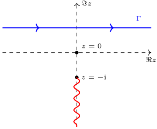
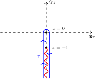
Figure 4. The integration contour $\Gamma$ for (6.7) shown in blue with branch cut in red. On the left our choice for $x<0$ and on the right for $x>0$.

Computing the residue and parametrizing the integral along the branch cut, one then obtains the well-known solution formula

$$\phi(x)=c\Bigg{(}\sqrt{3}\bigg{[}1+x \,-\frac{1}{\pi}\int_{0}^{\infty}\left\{\frac{1}{1-L(w)}-1-\frac{3}{w^{2}}\right\}\frac{{\mathrm{d}}w}{1+w^{2}}\bigg{]}$$

$$\,+\frac{\pi}{2}\mathrm{e}^{-x}\int_{0}^{\infty}\frac{\mathrm{e}^{-xw}}{F(-\mathrm{i}-\mathrm{i}w)}\frac{{\mathrm{d}}w}{(2+w-\frac{1}{2}\ln(\frac{2+w}{w}))^{2}+\frac{\pi^{2}}{4}}\Bigg{)},\ \ x>0.$$

In summary of this short subsection, using scalar Hilbert boundary value problems we can solve integral equations of the form (6.2) by the Wiener-Hopf method. This method has found countless applications and is particularly well-suited for PDE problems with semi-infinite boundaries, e.g. the Sommerfeld diffraction problem, see for instance [Nob] and [Dav, Chapter $16$] for further details.

6.2. The integrable systems revolution of the late 1960s

The classical (think of Euler, Hamilton, Jacobi, Liouville, Neumann and Kowaleskaya) field of integrable systems found renewed interest in the late 1960s when it became clear that several nonlinear PDEs in $1+1$ dimensions can be integrated by the inverse scattering method. Examples are the Kortweg-de Vries equation, the nonlinear Schrödinger equation (NLS), and the sine-Gordon equation, among many others. Important early contributions to this remarkable technique are due to Gardner, Green, Kruskal, and Miura [GGKM], due to Lax [Lax], due to Faddeev, Zakharov [ZF], and due to Shabat, Zakharov [ZS]. For a solid first introduction to the inverse scattering method we refer the interested reader to the monographs [NMPZ, AC, BDT, FT], here we shall discuss only one example and showcase the appearance of Riemann-Hilbert techniques: Consider the defocusing NLS

$$\mathrm{i}y_{t}+y_{xx}-2|y|^{2}y=0,\ \ \ \ y=y(x,t):\mathbb{R}^{2}\rightarrow\mathbb{C}.\vskip 3.0pt plus 1.0pt minus 1.0pt$$ (6.8)

How do we solve the corresponding initial value problem with Cauchy data $y(x,0)=y_{0}(x)\in\mathcal{S}(\mathbb{R})$ in the Schwartz space on the real line? Well, one first computes the reflection coefficient $r(z)\in\mathcal{S}(\mathbb{R})$ associated to $y_{0}$ through the direct scattering transform. There is not much freedom in this computation as the map $y_{0}\rightarrow r$ is a bijection from $\mathcal{S}(\mathbb{R})$ onto $\mathcal{S}(\mathbb{R})\cap\{r:\,\sup_{z\in\mathbb{R}}|r(z)|<1\}$, see [BC]. After that, one considers the so-called inverse scattering problem which is most conveniently formulated as the following Hilbert boundary value problem - this insight grew out of the works by Manakov, Shabat and Zakharov in the mid 1970s:

Hilbert Boundary Value Problem 6.2.

For any $x\in\mathbb{R}$ and $t>0$, determine $X(z)=X(z;x,t)\in\mathbb{C}^{2\times 2}$ such that

1. $X(z)$ is analytic in $\mathbb{C}\setminus\mathbb{R}$ and extends continuously from either side to the real axis.

2. On the real axis, the pointwise limits

   $$X_{\pm}(z):=\lim_{\epsilon\downarrow 0}X(z\pm\mathrm{i}\epsilon)$$

   satisfy the boundary condition $X_{+}(z)=X_{-}(z)G(z)$ with

   $$z\in\mathbb{R}:\ \ \ \ \ G(z)=\begin{bmatrix}1-|r(z)|^{2}&-\bar{r}(z)\mathrm{e}^{-2\mathrm{i}(2tz^{2}+xz)}\vskip 3.0pt plus 1.0pt minus 1.0pt\\ r(z)\mathrm{e}^{2\mathrm{i}(2tz^{2}+xz)}&1\end{bmatrix}\in\textnormal{GL}(2,\mathbb{C}).$$ (6.9)

3. Near $z=\infty$ we enforce the asymptotic behavior

   $$X(z)=\mathbb{I}+X_{1}z^{-1}+X_{2}z^{-2}+\mathcal{O}\big{(}z^{-3}\big{)},\ \ \ \ \ |z|\rightarrow\infty;\ \ \ \ X_{k}=X_{k}(x,t)=\big{[}X_{k}^{ij}(x,t)\big{]}_{i,j=1}^{2},$$

   where $\mathbb{I}\in\textnormal{GL}(2,\mathbb{C})$ is the identity matrix.

Indeed, provided this problem is solvable, its (unique) solution solves the PDE (6.8) with initial condition $y(x,0)=y_{0}(x)$ via the formula

$$y(x,t)=2\mathrm{i}X_{1}^{12}(x,t).$$ (6.10)

In order to arrive at (6.10) we use a slight modification of Plemelj’s argument that lead him to the linear system (4.19): The jump matrix $G(z),z\in\Gamma$ in Problem 4.1 was piecewise constant whereas (6.9) presents us with the other extreme, namely a jump matrix which depends on $z,x$ and $t$. However, assuming that Problem 6.2 is solvable, we can define

$$Y(z)\equiv Y(z;x,t):=X(z;x,t)\mathrm{e}^{-\mathrm{i}(2tz^{2}+xz)\sigma_{3}},\ \ \ \ z\in\mathbb{C}\setminus\mathbb{R},$$

and then conclude that both,

$$A(z):=\frac{\partial Y}{\partial x}(z)(Y(z))^{-1}\ \ \ \ \textnormal{and}\ \ \ \ B(z):=\frac{\partial Y}{\partial t}(z)(Y(z))^{-1},\ \ \ \ (z,x,t)\in\mathbb{C}\times\mathbb{R}\times(0,\infty)$$ (6.11)

are single-valued, entire functions in $z\in\mathbb{C}$. Moreover, using Problem 6.2, condition (3) and Liouville’s theorem we obtain the explicit formulæ

$$A(z)\equiv A(z;x,t)= \,-\mathrm{i}z\sigma_{3}+2\mathrm{i}\begin{bmatrix}0&X_{1}^{12}\vskip 3.0pt plus 1.0pt minus 1.0pt\\ -X_{1}^{21}&0\end{bmatrix},$$

$$B(z)\equiv B(z;x,t)= \,-2\mathrm{i}z^{2}\sigma_{3}+4\mathrm{i}z\begin{bmatrix}0&X_{1}^{12}\vskip 3.0pt plus 1.0pt minus 1.0pt\\ -X_{1}^{21}&0\end{bmatrix}+4\mathrm{i}\begin{bmatrix}-X_{1}^{12}X_{1}^{21}&X_{2}^{12}-X_{1}^{12}X_{1}^{22}\vskip 3.0pt plus 1.0pt minus 1.0pt\\ -X_{2}^{12}+X_{1}^{21}X_{1}^{11}&X_{1}^{21}X_{1}^{12}\end{bmatrix},$$

in term of the matrix coefficients $X_{k}^{ij}=X_{k}^{ij}(x,t)$ and the third Pauli matrix $\sigma_{3}:=\bigl{[}\begin{smallmatrix}1&0\\ 0&-1\end{smallmatrix}\bigr{]}$. The overdetermined system (6.11) forms one of the celebrated Lax pairs for the PDE (6.8), indeed writing out the Frobenius integrability condition for $\frac{\partial Y}{\partial x}=AY,\frac{\partial Y}{\partial t}=BY$, equivalently the compatibility condition

$$AB-BA=\frac{\partial B}{\partial x}-\frac{\partial A}{\partial t},$$

we find entrywise the coupled partial differential equations

$$2\mathrm{i}(X_{1}^{12})_{x}= \,\,4(X_{2}^{12}-X_{1}^{12}X_{1}^{22}),\ \ \ \ \ \ \ -2\mathrm{i}(X_{1}^{21})_{x}=4(X_{2}^{21}-X_{1}^{21}X_{1}^{11}),$$

$$4\mathrm{i}(X_{2}^{12}-X_{1}^{12}X_{1}^{22})_{x}-2\mathrm{i}(X_{1}^{12})_{t}= \,-16X_{1}^{12}X_{1}^{21}X_{1}^{12},$$

$$-4\mathrm{i}(X_{2}^{21}-X_{1}^{21}X_{1}^{11})_{x}+2\mathrm{i}(X_{1}^{21})_{t}= \,-16X_{1}^{21}X_{1}^{12}X_{1}^{21}.$$

However, the coefficients back in condition (3) of Problem 6.2 satisfy $\mathop{\mathrm{tr}}\limits X_{1}=0$ and $X_{k}^{11}=\overline{X_{k}^{22}},X_{k}^{21}=\overline{X_{k}^{12}},k\in\mathbb{Z}_{\geq 1}$. Thus the above four coupled equations boil down to

$$y_{x}=4(X_{2}^{12}-X_{1}^{12}X_{1}^{22}),\ \ \ \ \ \ \ \ \ \ 2|y|^{2}y=4(X_{2}^{12}-X_{1}^{12},X_{1}^{22})_{x}+\mathrm{i}y_{t},$$

where we used (6.10) and so after substitution into one another

$$\mathrm{i}y_{t}+y_{xx}-2|y|^{2}y=0,$$

which is the defocusing NLS (6.8). Summarizing this short computation, provided Problem 6.2 is solvable, the linear Hilbert boundary value problem solves the nonlinear evolution equation (6.8) via the formula (6.10). This is a far reaching generalization of Plemelj’s idea to construct solutions of certain linear ODE systems in terms of solutions of Hilbert boundary value problems, nevertheless the common approach to both problems is clearly visible. In Section 7 below we will address the solvability question of Problem 6.2 which requires a different toolset than the one used by Plemelj in his analysis of Problem 4.1.

6.3. Painlevé special function theory

Painlevé functions form a family of special functions which is widely regarded as the substitute for classical special functions in nonlinear mathematical physics (such Airy, Bessel or Hypergeometric functions). Although Painlevé transcendents are non-expressible in terms of a finite number of contour integrals over elementary, elliptic or finite genus algebraic functions, several of their key analytic and asymptotic properties can be studied with Riemann-Hilbert techniques. These techniques are therefore in a way the analogues of contour integral representations and steepest descent asymptotic methods used in the analysis of classical special functions. For a comprehensive introduction to Painlevé special functions and Riemann-Hilbert techniques associated with them, including several references to their applications in mathematical physics, we recommend the two monographs [GLS, FIKN]. Similar to the last subsection we will showcase the Riemann-Hilbert approach to one particular Painlevé equation, namely

$$u_{xx}=xu+2u^{3},\ \ \ \ u=u(x):\mathbb{R}\rightarrow\mathbb{R},$$ (6.12)

the homogeneous Painlevé-II equation, which, to a certain extent, is a nonlinear Airy equation. How do we solve the associated initial value problem? Well, in the Riemann-Hilbert approach to (6.12) one parametrizes the solutions $u=u(x)$ of (6.12) not in terms of Cauchy data, but in terms of the monodromy data of an associated linear system of ordinary differential equations: Precisely, define the generically two-dimensional real manifold

$$\mathcal{S}:=\big{\{}(s_{1},s_{2},s_{3})\in\mathbb{C}^{3}:\,s_{1}-s_{2}+s_{3}+s_{1}s_{2}s_{3}=0,\ \ s_{1}=\bar{s}_{3},\ \ s_{2}=\bar{s}_{2}\big{\}},$$

and introduce with $s_{k+3}=-s_{k},k=1,2,3$ for $k=1,\ldots,6$ the triangular matrices

$$S_{k}:=\begin{bmatrix}1&0\\ s_{k}&0\end{bmatrix},\ \ k\equiv 1\mod 2;\ \ \ \ \ \ \ S_{k}:=\begin{bmatrix}1&s_{k}\\ 0&1\end{bmatrix},\ \ k\equiv 0\mod 2.$$

Now consider the below Hilbert boundary value problem.

Hilbert Boundary Value Problem 6.3.

For any $x\in\mathbb{R}$, determine $X(z)=X(z;x,s)\in\mathbb{C}^{2\times 2}$ with $s:=(s_{1},s_{2},s_{3})\in\mathcal{S}$ such that

1. $X(z)$ is analytic in $\mathbb{C}\setminus\bigcup_{i=1}^{6}\Gamma_{i}$ and continuous on the closed sectors $\overline{\Omega}_{i}$. Compare Figure 5 for the six rays $\Gamma_{i}$ and the sectors $\Omega_{i}$ in between them.

2. On the rays $\Gamma_{i},i=1,\ldots,6$ the pointwise limits

   $$X_{\pm}(z):=\lim_{\begin{subarray}{c}w\rightarrow z\\ w\in\Omega_{\pm}\end{subarray}}X(w),\ \ \ \Omega_{+}:=\Omega_{i+1},\ \ \ \Omega_{-}:=\Omega_{i},\ \ \ \Omega_{7}\equiv\Omega_{1},$$

   satisfy the boundary condition $X_{+}(z)=X_{-}(z)G(z)$ with

   $$z\in\Gamma_{i}:\ \ \ \ G(z)=\mathrm{e}^{-\theta(z,x)\sigma_{3}}S_{i}\,\mathrm{e}^{\theta(z,x)\sigma_{3}}\in\textnormal{GL}(2,\mathbb{C});\ \ \ \ \theta(z,x):=\mathrm{i}\left(\frac{4}{3}z^{3}+xz\right).$$

3. Near $z=\infty$ we enforce the asymptotic behavior

   $$X(z)=\mathbb{I}+X_{1}z^{-1}+X_{2}z^{-2}+\mathcal{O}\big{(}z^{-3}\big{)},\ \ \ |z|\rightarrow\infty;\ \ \ \ X_{k}=X_{k}(x,s)=\big{[}X_{k}^{ij}(x,s)\big{]}_{i,j=1}^{2}.$$

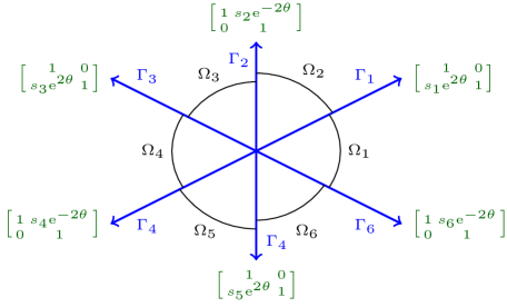
Figure 5. The oriented contour $\bigcup_{i=1}^{6}\Gamma_{i}$ in blue together with the sectors $\Omega_{i}$ in between. The six rays are $\Gamma_{i}=\{z\in\mathbb{C}:\,\textnormal{arg}\,z=\frac{\pi}{6}+\frac{\pi}{3}(i-1)\}$ and we indicate the values of $G(z)$ on them in green.

The route between Problem 6.3 and (6.12) goes as follows: for any choice of parameters $(s_{1},s_{2},s_{3})\in\mathcal{S}$ the Hilbert boundary value problem 6.3 is meromorphically with respect to $x$ solvable, cf. [BIK]. In turn the unique solution to said Problem leads to a solution of (6.12) via

$$u(x)\equiv u(x|s)=2X_{1}^{12}(x,s),$$ (6.13)

which is the analogue of the NLS formula (6.10). Additionally, (6.13) satisfies $\bar{u}(x)=u(\bar{x})$, i.e. the solution is real-valued on the real axis and conversely, every on the real axis real-valued solution of (6.12) admits a unique Riemann-Hilbert representation (6.13) for suitable $s$. In short, we do parametrize solutions of (6.12) in terms of the monodromy data $(s_{1},s_{2},s_{3})\in\mathcal{S}$ using a bijection between the initial value solution space of (6.12) and $\mathcal{S}$.

The derivation of (6.13), and thus the Riemann-Hilbert approach to the second Painlevé equation is due to Flaschka, Newell [FN] and Jimbo, Miwa, Ueno [JMU, JM1, JM2] in the early 1980s. In a nutshell, we use again Plemelj’s basic idea: suppose Problem 6.3 is solvable and set

$$Y(z)\equiv Y(z;s,s):=X(z;x,s)\mathrm{e}^{-\theta(z,x)\sigma_{3}},\ \ \ z\in\mathbb{C}\setminus\bigcup_{i=1}^{6}\Gamma_{i}.$$

Then both,

$$A(z):=\frac{\partial Y}{\partial z}(Y(z))^{-1}\ \ \ \ \ \ \textnormal{and}\ \ \ \ \ \ \ B(z):=\frac{\partial Y}{\partial x}(z)(Y(z))^{-1},\ \ \ \ \ (z,x)\in\mathbb{C}\times(\mathbb{R}\setminus D)$$

are single-valued, entire functions in $z\in\mathbb{C}$ away from a discrete set $D\subset\mathbb{R}$. Hence, using condition (3) in Problem 6.3 and Liouville’s theorem, we obtain the explicit formulæ

$$A(z)\equiv A(z;x,s)= \,\,-4\mathrm{i}z^{2}\sigma_{3}+8\mathrm{i}z\begin{bmatrix}0&X_{1}^{12}\vskip 3.0pt plus 1.0pt minus 1.0pt\\ -X_{1}^{21}&0\end{bmatrix}+\begin{bmatrix}-\mathrm{i}x-8\mathrm{i}X_{1}^{12}X_{1}^{21}&8\mathrm{i}(X_{2}^{12}-X_{1}^{12}X_{1}^{22})\vskip 3.0pt plus 1.0pt minus 1.0pt\\ -8\mathrm{i}(X_{2}^{21}-X_{1}^{21}X_{1}^{11})&\mathrm{i}x+8\mathrm{i}X_{1}^{21}X_{1}^{12}\end{bmatrix},$$

$$B(z)\equiv B(z;x,s)= \,\,-\mathrm{i}z\sigma_{3}+2\mathrm{i}\begin{bmatrix}0&X_{1}^{12}\vskip 3.0pt plus 1.0pt minus 1.0pt\\ -X_{1}^{21}&0\end{bmatrix},$$

in terms of the matrix coefficients $X_{k}$ and from those, reading the compatibility condition

$$AB-BA=\frac{\partial B}{\partial z}-\frac{\partial A}{\partial x},$$

entrywise, the following coupled ordinary differential equations,

$$(X_{1}^{12})_{x}= \,\,-2\mathrm{i}(X_{2}^{12}-X_{1}^{12}X_{1}^{22}),\ \ \ \ \ \ \ \ (X_{1}^{21})_{x}=2\mathrm{i}(X_{2}^{21}-X_{1}^{21}X_{1}^{11}),$$

$$-2(X_{2}^{12}-X_{1}^{12}X_{1}^{22})_{x}= \,\,X_{1}^{12}(-\mathrm{i}x-8\mathrm{i}X_{1}^{12}X_{1}^{21}),$$

$$-2(X_{2}^{21}-X_{1}^{12}X_{1}^{11})_{x}= \,\,X_{1}^{21}(\mathrm{i}x+8\mathrm{i}X_{1}^{21}X_{1}^{12}).$$

However Problem 6.3 also possesses certain implicit symmetries that yield $\mathop{\mathrm{tr}}\limits X_{1}=0$, $X_{k}^{12}=(-1)^{k-1}X_{k}^{21},k\in\mathbb{Z}_{\geq 1}$ and which simplify the above four equations to

$$u_{x}=-4\mathrm{i}(X_{2}^{12}-X_{1}^{12}X_{1}^{22}),\ \ \ \ \ \ \ \ \ \mathrm{i}(xu+2u^{3})=4(X_{2}^{12}-X_{1}^{12}X_{1}^{22})_{x},$$

where we used (6.13). Substituting both equations into one another we find

$$u_{xx}=xu+2u^{3},$$

and therefore Painlevé-II (6.12). In summary, the Hilbert boundary value problem 6.3 linearizes the nonlinear Painlevé-II ODE and therefore shares common ground with (4.19) and (6.8). Before we move to our next example it will be important to mention that the monodromy data $s=(s_{1},s_{2},s_{3})\in\mathcal{S}$ forms a complete set of first integrals for (6.12). Building on this feature, one can in principle use the highly transcendental equations

$$s_{i}=s_{i}(x,u,u_{x})\equiv\textnormal{const},\ \ \ \ i=1,2,3$$ (6.14)

in the further analysis of the Painlevé-II transcendents. This idea is at the heart of the isomonodromy method and the corresponding direct monodromy approach to Painlevé equations as pioneered by Its, Novokshenov, Kapaev and Kitaev in the mid 1980s, cf. [IN] or [FIKN, Chapter $7$]. Their approach relies on complex WKB techniques applied to Problem 6.3 and certain a priori assumptions on the behavior of $u=u(x)$. We will later on highlight a different method, the inverse monodromy approach, a.k.a. Deift-Zhou method [DZ], which (in the extended form of Deift, Venakides, Zhou [DVZ]) has become extremely popular in nonlinear mathematical physics since its discovery back in 1993. This method is suitable for the analysis of Painlevé functions and other problems that we are about to discuss.

6.4. The Heisenberg antiferromagnet

Our next example is concerned with a quantum mechanical model for an antiferromagnetic spin chain. It was introduced by Lieb, Schultz and Mattis [LSM] in 1961 and is known as the spin-$\frac{1}{2}$XY model, equivalently the Heisenberg XX0 antiferromagnet. In this model $\frac{1}{2}$-spins are situated on a one-dimensional periodic and isotropic lattice, we allow only nearest neighbor interactions between the spins, neighboring spins tend to point in opposite directions and a moderate external transverse magnetic field influences the spins. Subject to these four constraints the Hamiltonian of the model equals, cf. [LSM, $(2.1)$],

$$\mathscr{H}:=\sum_{j=1}^{N}\sigma_{j}^{x}\sigma_{j+1}^{x}+\sum_{j=1}^{N}\sigma_{j}^{y}\sigma_{j+1}^{y}-h\sum_{j=1}^{N}\sigma_{j}^{z},$$

where we set the nearest neighbor coupling constant to unity, $0<h<2$ denotes the strength of the external magnetic field and

$$\sigma^{x}\equiv\sigma_{1}:=\begin{bmatrix}0&1\\ 1&0\end{bmatrix},\ \ \ \sigma^{y}\equiv\sigma_{2}:=\begin{bmatrix}0&-\mathrm{i}\\ \mathrm{i}&0\end{bmatrix},\ \ \ \sigma^{z}=\sigma_{3}=\begin{bmatrix}1&0\\ 0&-1\end{bmatrix},$$

are the Pauli spin matrices. The paper [LSM] computed the model’s ground state, all elementary excitations and the free energy through creation-annihilation operator techniques. Here we shall focus on an important correlation function, the so-called emptiness formation probability

$$P_{n}:=\textnormal{Prob}\big{\{}\textnormal{there are}\,\,n\in\mathbb{Z}_{\geq 1}\,\,\textnormal{adjacent parallel spins up in the ground state}\big{\}},$$

which was evaluated in the thermodynamic limit $N\rightarrow\infty$ for fixed $h$ in [EFIK, $(10.2),(10.3)$] by the quantum inverse scattering method. The result is the Fredholm determinant formula

$$P_{n}=\det\big{(}1-U_{n}\upharpoonright_{L^{2}(J,{\mathrm{d}}x)}\big{)}:=\sum_{k=0}^{\infty}\frac{(-1)^{k}}{k!}\int_{J}\cdots\int_{J}\det\big{[}U_{n}(x_{i},x_{j})\big{]}_{i,j=1}^{k}{\mathrm{d}}x_{1}\cdots{\mathrm{d}}x_{k},$$ (6.15)

where $U_{n}:L^{2}(J,{\mathrm{d}}x)\rightarrow L^{2}(J,{\mathrm{d}}x)$ denotes the trace class operator with kernel

$$U_{n}(\lambda,\mu):=\frac{1}{2\pi\mathrm{i}}\frac{1}{\sinh(\lambda-\mu)}\left\{1-\left(\frac{\mathrm{e}^{2\lambda}+\mathrm{i}}{\mathrm{e}^{2\lambda}-\mathrm{i}}\right)^{n}\left(\frac{\mathrm{e}^{2\mu}-\mathrm{i}}{\mathrm{e}^{2\mu}+\mathrm{i}}\right)^{n}\right\},$$

acting on the interval $J:=(-\Lambda,\Lambda)\subset\mathbb{R}$ with $\cosh 2\Lambda=\frac{2}{h}>1$. The central analytical challenges associated with $P_{n}$ consist in accessing its large $n$ asymptotic behavior and in identifying an underlying integrable system for it. Both questions yield physically relevant information for the spin chain model, so how do we go about them? First, one factorizes the operator $U_{n}$ as

$$U_{n}=E^{-1}D_{n}K_{n}(E^{-1}D_{n})^{-1},$$ (6.16)

where $D_{n}$ denotes multiplication $(D_{n}f)(z):=z^{-\frac{n}{2}}\mathrm{e}^{\lambda(z)}(z+\mathrm{i})$ with the invertible change of variables $\lambda=\lambda(z)$ defined as

$$z=:-\mathrm{i}\frac{\mathrm{e}^{2\lambda}-\mathrm{i}}{\mathrm{e}^{2\lambda}+\mathrm{i}},\ \ \ \ z(J)=\big{\{}z\in\mathbb{C}:\,|z|=1,\ \textnormal{arg}\,\in(\phi,2\pi-\phi)\big{\}},\ \ \mathrm{e}^{\mathrm{i}\phi}=z(-\Lambda),\ \phi\in\left(\frac{\pi}{2},\pi\right),$$ (6.17)

$E$ is the evaluation $(Ef)(z):=f(\lambda(z))$ and $K_{n}:L^{2}(\Gamma,|{\mathrm{d}}z|)\rightarrow L^{2}(\Gamma,|{\mathrm{d}}z|)$ the trace class operator with kernel

$$K_{n}(z,w):=\frac{z^{\frac{n}{2}}w^{-\frac{n}{2}}-z^{-\frac{n}{2}}w^{\frac{n}{2}}}{2\pi\mathrm{i}(z-w)},$$ (6.18)

acting on the arc $\Gamma:=z(J)\subset\mathbb{C}$ defined in (6.17) and shown in Figure 6. Second, one notices that (6.18) is a particular instance of an integrable kernel, i.e. a kernel of the form

$$K(x,y)=\frac{\sum_{j=1}^{N}f_{j}(x)g_{j}(y)}{x-y},\ \ \ \ x,y\in\Gamma\ \ \ \ \ \ \ \textnormal{with}\ \ \ \ \ \ \ \sum_{j=1}^{N}f_{j}(x)g_{j}(x)=0,\ \ x\in\Gamma,$$

for some functions $f_{j},g_{j}\in L^{\infty}(\Gamma,|{\mathrm{d}}z|),1\leq j\leq N$. The associated integral operator $K:L^{2}(\Gamma,|{\mathrm{d}}z|)\rightarrow L^{2}(\Gamma,|{\mathrm{d}}z|)$ has many remarkable properties, most importantly $(1-K)^{-1}$ (if existent) can be computed in terms of the solution of a naturally associated Hilbert boundary value problem. This insight was formalized in the important 1990 paper [IIKS] by Its, Izergin, Korepin and Slavnov, see [D0] for a concise review, and reads in case of (6.18) as follows:

Hilbert Boundary Value Problem 6.4.

For any $n\in\mathbb{Z}_{\geq 1}$ and $0<h<2$, determine $X(z)=X(z;n,h)\in\mathbb{C}^{2\times 2}$ such that

1. $X(z)$ is analytic in $\mathbb{C}\setminus\Gamma$ and extends continuously from either side to $\Gamma\setminus\{\xi,\bar{\xi}\}$. See Figure 6 for the jump contour $\Gamma$ and its endpoints $\xi$ and $\bar{\xi}$.

2. On the arc $\Gamma\subset\mathbb{C}$ the pointwise limits

   $$X_{\pm}(z):=\lim_{\begin{subarray}{c}w\rightarrow z\\ w\in\Omega_{\pm}\end{subarray}}X(w),$$

   satisfy the boundary condition $X_{+}(z)=X_{-}(z)G(z)$ with

   $$z\in\Gamma:\ \ \ \ \ \ G(z)=\begin{bmatrix}0&-z^{n}\\ z^{-n}&2\end{bmatrix}\in\textnormal{GL}(2,\mathbb{C}).$$

   

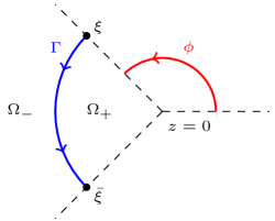
   Figure 6. The oriented contour $\Gamma$ in blue together with the sectors $\Omega_{\pm}$. The endpoints are $\xi:=\mathrm{e}^{\mathrm{i}\phi}=z(-\Lambda),\bar{\xi}=\mathrm{e}^{-\mathrm{i}\phi}$ and the angle $\phi$ in (6.17) is shown in red.

3. In a small neighborhood of $z=\xi$ and $z=\bar{\xi}$ we impose the blow-up constraint

   $$\|X(z)\|\leq C\,\big{|}\ln\left|\frac{z-\xi}{z-\bar{\xi}}\right|\big{|},\ \ \ \ \ \ C>0.$$

4. Near $z=\infty$ we require the asymptotic normalization

   $$X(z)=\mathbb{I}+X_{1}z^{-1}+\mathcal{O}\big{(}z^{-2}\big{)},\ \ \ |z|\rightarrow\infty;\ \ \ X_{k}=X_{k}(n,h)=\big{[}X_{k}^{ij}(n,h)\big{]}_{i,j=1}^{2}.$$

Problem 6.4 and the emptiness formation probability (6.15) are related in the following way: as shown in [DIZ, Proposition $6.12$], the Hilbert boundary value problem 6.4 is uniquely solvable for any $n\in\mathbb{Z}_{\geq 1},h\in(0,2)$ and its solution leads to the below recursion for $P_{n}$,

$$\frac{P_{n+1}}{P_{n}}=X^{11}(0;n,h),$$ (6.19)

in terms of the $(11)$-entry of the solution to Problem 6.4. This identity is more complicated than the representation formulæ (6.10), (6.13) and its derivation does not use a Lax pair as in the NLS or Painlevé-II example. Nevertheless, (6.19) enables us to use Riemann-Hilbert techniques in the analysis of the spin chain model, i.e. Plemelj’s basic idea occurs once more.

In order to obtain (6.19), we first use the operator factorization (6.16) and Sylvester’s determinant identity,

$$P_{n}=\det\big{(}1-U_{n}\upharpoonright_{L^{2}(J,{\mathrm{d}}x)}\big{)}=\det\big{(}1-K_{n}\upharpoonright_{L^{2}(\Gamma,|{\mathrm{d}}z|)}\big{)}.$$

Next we realize that

$$K_{n+1}(z,w)=K_{n}(z,w)+\frac{1}{2\pi\mathrm{i}}z^{\frac{n}{2}}w^{-\frac{n}{2}-1}=:K_{n}(z,w)+(\alpha_{n}\otimes\beta_{n})(z,w),$$

where $\alpha_{n}\otimes\beta_{n}$ is the finite rank integral operator on $L^{2}(\Gamma,|{\mathrm{d}}z|)$ with kernel $(\alpha_{n}\otimes\beta_{n})(z,w)=\alpha_{n}(z)\beta_{n}(w)$ in terms of $\alpha_{n}(z):=\frac{1}{2\pi\mathrm{i}}z^{\frac{n}{2}}$ and $\beta_{n}(w):=w^{-\frac{n}{2}-1}$. But [IIKS] showed that Problem 6.4 is solvable if and only if $(1-K_{n})^{-1}$ exists, so we can further simplify (6.15),

$$P_{n+1}=\det\big{(}1-K_{n}-\alpha_{n}\otimes\beta_{n}\upharpoonright_{L^{2}(\Gamma,|{\mathrm{d}}z|)}\big{)}=P_{n}\,\det\big{(}1-(1-K_{n})^{-1}(\alpha_{n}\otimes\beta_{n})\upharpoonright_{L^{2}(\Gamma,|{\mathrm{d}}z|)}\big{)},$$

and evaluate the remaining Fredholm determinant with the general theory of finite rank operators,

$$\frac{P_{n+1}}{P_{n}}=1-\int_{\Gamma}\big{(}(1-K_{n})^{-1}\alpha_{n}\big{)}(z)z^{-\frac{n}{2}}\,\frac{{\mathrm{d}}z}{z}.$$ (6.20)

At this point we use the general fact, cf. [IIKS] or (7.5) below, that the solution of Problem 6.4 can be expressed in integral form, similar to Plemelj’s quasi-regular equation (4.4),

$$X(z)=\mathbb{I}-\int_{\Gamma}F(w)g^{\top}(w)\frac{{\mathrm{d}}w}{w-z},\ \ z\notin\Gamma;\ \ \ \ \ F_{i}(z):=\big{(}(1-K_{n})^{-1}f_{i}\big{)}(z),\ \ z\in\Gamma,$$

with $F(z):=(F_{1}(z),F_{2}(z))^{\top},g(z):=(g_{1}(z),g_{2}(z))^{\top}$ and

$$f_{1}(z):=\frac{1}{2\pi\mathrm{i}}z^{\frac{n}{2}},\,\,f_{2}(z):=-\frac{1}{2\pi\mathrm{i}}z^{-\frac{n}{2}},\,\,g_{1}(z):=z^{-\frac{n}{2}},\,\,g_{2}(z):=z^{\frac{n}{2}},\ \ \ \ \ \textnormal{arg}\,z\in(\phi,2\pi-\phi).$$

Setting $z=0$ in the integral formula for $X(z)$ and comparing with (6.20) yields

$$\frac{P_{n+1}}{P_{n}}=X^{11}(0;n,h),$$

i.e. the representation (6.19). In summary, the Hilbert boundary value problem 6.4 linearizes to a certain extent (note that (6.19) is a formula for the discrete logarithmic derivative of $P_{n}$ and not $P_{n}$ itself) the highly transcendental Fredholm determinant (6.15). We will display the usefulness of (6.19) after the next subsection.

6.5. Invariant random matrix models

Our fifth and last example in this section concerns the statistical behavior of eigenvalues of a random matrix drawn from a particular ensemble. We will focus on an especially well-studied ensemble, the so called unitary ensemble $\mathcal{M}(n)$ of $n\times n$ Hermitian matrices equipped with the probability measure

$$P(M)\,{\mathrm{d}}M=\frac{1}{Z_{n,N}}\,\mathrm{e}^{-N\textnormal{tr}\,V(M)}\,{\mathrm{d}}M,\ \ \ \ \ \ Z_{n,N}:=\int_{\mathcal{M}(n)}\mathrm{e}^{-N\textnormal{tr}\,V(M)}\,{\mathrm{d}}M<\infty.$$ (6.21)

Here, ${\mathrm{d}}M$ is the Haar measure on $\mathcal{M}(n)\simeq\mathbb{R}^{n^{2}}$, $N\in\mathbb{Z}_{\geq 1}$ a scaling parameter and $V:\mathbb{R}\rightarrow\mathbb{R}$ assumed to be real analytic satisfying the growth condition

$$\frac{V(x)}{\ln(x^{2}+1)}\rightarrow\infty\ \ \ \ \textnormal{as}\ \ \ |x|\rightarrow\infty,$$

in order to ensure that (6.21) is a bona fide model. Measures of the form (6.21) appeared seemingly first in the work of Hurwitz in 1897 [Hu], they appeared in a paper by Wishart in 1928 [Wish] and in particular in Wigner’s work in the 1950s [Wig] who used them to model the statistical properties of highly excited energy levels of complex nuclei, see [DF] for an excellent historic review of the subject. A classical fact of the setup (6.21) is that the location of the eigenvalues of a matrix drawn from the unitary ensemble form a determinantal point process. This detail allows us to compute several of the key statistical properties of the random matrix model from the underlying Christoffel-Darboux kernel

$$K_{n,N}(x,y)=\mathrm{e}^{-\frac{N}{2}V(x)}\mathrm{e}^{-\frac{N}{2}V(y)}\sum_{k=0}^{N-1}\frac{1}{h_{k}^{2}}\,p_{k}(x)p_{k}(y),\ \ \ x,y\in\mathbb{R},$$ (6.22)

which is defined in terms of the sequence $\{p_{n}(x)\}_{n=0}^{\infty}\subset\mathbb{C}[x]$ of monic orthogonal polynomials with respect to the measure $\mathrm{e}^{-NV(x)}\,{\mathrm{d}}x$ supported on $\mathbb{R}$, i.e.

$$\int_{-\infty}^{\infty}p_{j}(x)p_{k}(x)\mathrm{e}^{-NV(x)}\,{\mathrm{d}}x=h_{k}^{2}\delta_{jk},\ \ \ \ \ \ p_{j}(x)=x^{j}+\mathcal{O}(x^{j-1}).$$

Indeed, focusing on one important statistical property of the model (6.21), the gap probability,

$$E_{n}(s):=\textnormal{Prob}\big{\{}M\in\mathcal{M}(n)\ \textnormal{has no eigenvalues in the interval}\,(-s,s)\subset\mathbb{R},s>0\big{\}},$$

admits the determinantal representation

$$E_{n}(s)=\det\big{(}1-K_{n,N}\upharpoonright_{L^{2}((-s,s),{\mathrm{d}}x)}\big{)},$$ (6.23)

where $K_{n,N}$ is the finite rank operator with kernel (6.22). Formula (6.23) goes back to the seminal works of Dyson, Gaudin and Mehta in the 1970s and it is the analogue of the emptiness formation probability formula (6.15) in the spin chain model. Thus, in order to compute the likelihood of large eigenvalue gaps from (6.23), we need to carefully analyze the asymptotic behavior of the kernel (6.22). However, in all but a few cases, the orthogonal polynomials that built the kernel are not known explicitly, so how can we effectively use (6.22)? Well, as it happens, the polynomials $\{p_{n}(x)\}_{n=0}^{\infty}$ and the kernel $K_{n,N}(x,y)$ itself can be characterized through a Hilbert boundary value problem. This remarkable fact was discovered by Fokas, Its and Kitaev [FIK1, FIK2] in the early 1990s and the details are as follows:

Hilbert Boundary Value Problem 6.5.

For any $n\in\mathbb{Z}_{\geq 0}$ and $N\in\mathbb{Z}_{\geq 1}$, determine $X(z)=X(z;n,N)\in\mathbb{C}^{2\times 2}$ such that

1. $X(z)$ is analytic in $\mathbb{C}\setminus\mathbb{R}$ and extends continuously from either side to the real axis.

2. On the real axis, the pointwise limits

   $$X_{\pm}(z):=\lim_{\epsilon\downarrow 0}X(z\pm\mathrm{i}\epsilon)$$

   satisfy the boundary condition $X_{+}(z)=X_{-}(z)G(z)$ with

   $$z\in\mathbb{R}:\ \ \ \ \ \ G(z)=\begin{bmatrix}1&\mathrm{e}^{-NV(z)}\\ 0&1\end{bmatrix}\in\textnormal{GL}(2,\mathbb{C}).$$ (6.24)

3. Near $z=\infty$ we enforce the asymptotic behavior

   $$X(z)=\Big{(}\mathbb{I}+X_{1}z^{-1}+\mathcal{O}\big{(}z^{-2}\big{)}\Big{)}z^{n\sigma_{3}},\ \ |z|\rightarrow\infty.$$

Fokas, Its and Kitaev showed that this problem is uniquely solvable for a given $n\in\mathbb{Z}_{\geq 0}$ if and only if the $n$th monic orthogonal polynomial $p_{n}(x)$ exists. Moreover, in case when its solvability is ensured, then we have for any $x,y\in\mathbb{R}$,

$$p_{n}(x)=X^{11}(x;n,N)\ \ \ \ \textnormal{and}\ \ \ \ K_{n,N}(x,y)=\mathrm{e}^{-\frac{N}{2}V(x)}\left[\frac{(X_{+}(y))^{-1}X_{+}(x)}{2\pi\mathrm{i}(x-y)}\right]^{21}\mathrm{e}^{-\frac{N}{2}V(y)},$$ (6.25)

in terms of the $(11)$-entry of $X(z)$ for the polynomial and the $(21)$-entry of the matrix product for the kernel. Here are the details: assuming the solvability of Problem 6.5, the jump constraint (6.24) states that the first column of $X(z)$ is an entire function,

$$X_{+}^{11}(z)=X_{-}^{11}(z),\ \ \ X_{+}^{21}(z)=X_{-}^{21}(z),\ \ \ \ X_{+}^{12}(z)= \,\,X_{-}^{12}(z)+X_{-}^{11}(z)\mathrm{e}^{-NV(z)}$$ (6.26)

$$X_{+}^{22}(z)= \,\,X_{-}^{22}(z)+X_{-}^{21}(z)\mathrm{e}^{-NV(z)},\ \ z\in\mathbb{R}.$$

But the asymptotic normalization at $z=\infty$ enforces at the same time that

$$X^{11}(z)=z^{n}+X_{1}^{11}z^{n-1}+\mathcal{O}\big{(}z^{n-2}\big{)},\ \ \ \ \ X^{21}(z)=X_{1}^{21}z^{n-1}+\mathcal{O}\big{(}z^{n-2}\big{)},$$

and

$$X^{12}(z)=X_{1}^{12}z^{-n-1}+\mathcal{O}\big{(}z^{-n-2}\big{)},\ \ \ \ \ \ X^{22}(z)=z^{-n}+X_{1}^{22}z^{-n-1}+\mathcal{O}\big{(}z^{-n-2}\big{)}.$$ (6.27)

Hence, $X^{11}(z)$ must be a monic polynomial of degree $n$ and $X^{21}(z)$ a polynomial of degree at most $n-1$ by Liouville’s theorem. Returning with this information to (6.26) and using the Plemelj-Sokhotski formula we then find for $z\in\mathbb{C}\setminus\mathbb{R}$,

$$X^{12}(z)=\frac{1}{2\pi\mathrm{i}}\int_{-\infty}^{\infty}X^{11}(w)\mathrm{e}^{-NV(w)}\frac{{\mathrm{d}}w}{w-z}\ \ \ \textnormal{and}\ \ \ X^{22}(z)=\frac{1}{2\pi\mathrm{i}}\int_{-\infty}^{\infty}X^{21}(w)\mathrm{e}^{-NV(w)}\frac{{\mathrm{d}}w}{w-z}.$$ (6.28)

But geometric progression yields for $z\notin\mathbb{R}$,

$$X^{12}(z)=-\frac{1}{2\pi\mathrm{i}}\sum_{k=0}^{n-1}\frac{1}{z^{k+1}}\int_{-\infty}^{\infty}X^{11}(w)w^{k}\mathrm{e}^{-NV(w)}\,{\mathrm{d}}w+\frac{z^{-n}}{2\pi\mathrm{i}}\int_{-\infty}^{\infty}X^{11}(w)\mathrm{e}^{-NV(w)}\frac{w^{n}}{w-z}\,{\mathrm{d}}w$$

and thus after comparison with (6.27)

$$\int_{-\infty}^{\infty}X^{11}(w)w^{k}\mathrm{e}^{-NV(w)}\,{\mathrm{d}}w=0,\ \ \ k=0,\ldots,n-1.$$

Since $X^{11}(z)$ has already been found to be a monic polynomial, it must therefore be the $n$th monic orthogonal polynomial $p_{n}(x)$ for the measure $\mathrm{e}^{-NV(x)}\,{\mathrm{d}}x$ on $\mathbb{R}$, so the first identity in (6.25) follows. The kernel identity is slightly more complicated and involves $X^{21}(z)$: From the integral formula of $X^{22}(z)$ in (6.28), by geometric progression for $z\in\mathbb{C}\setminus\mathbb{R}$,

$$X^{22}(z)=-\frac{1}{2\pi\mathrm{i}}\sum_{k=0}^{n-2}\frac{1}{z^{k+1}}\int_{-\infty}^{\infty}X^{21}(w)w^{k}\mathrm{e}^{-NV(w)}\,{\mathrm{d}}w+\frac{z^{-n+1}}{2\pi\mathrm{i}}\int_{-\infty}^{\infty}X^{21}(w)\mathrm{e}^{-NV(w)}\frac{w^{n-1}}{w-z}\,{\mathrm{d}}w,$$

so after comparison with (6.27),

$$\int_{-\infty}^{\infty}X^{21}(w)w^{k}\mathrm{e}^{-NV(w)}\,{\mathrm{d}}w=0,\ \ \ k=0,\ldots,n-2;\ \ \ \ \frac{\mathrm{i}}{2\pi}\int_{-\infty}^{\infty}X^{21}(w)w^{n-1}\mathrm{e}^{-NV(w)}\,{\mathrm{d}}w=1.$$

This shows that $X^{21}(z)$ must be proportional to $p_{n-1}(z)$, i.e. we have for some $\gamma_{n-1}\in\mathbb{C}\setminus\{0\}$,

$$X^{21}(z)=\gamma_{n-1}p_{n-1}(z),\ \ \ z\in\mathbb{C},$$

and thus by orthogonality and the very definition of the sequence $\{p_{n}(x)\}_{n=0}^{\infty}$,

$$-2\pi\mathrm{i}=\int_{-\infty}^{\infty}X^{21}(w)w^{n-1}\mathrm{e}^{-NV(w)}\,{\mathrm{d}}w=\gamma_{n-1}\int_{-\infty}^{\infty}p_{n-1}^{2}(w)\mathrm{e}^{-NV(w)}\,{\mathrm{d}}w=\gamma_{n-1}h_{n-1}^{2}.$$

Next we note that any solution of Problem 6.5 must be unimodular in the entire plane, i.e. $\det X(z)\equiv 1$ for all $z\in\mathbb{C}$. Indeed, the function $\det X(z)$ is analytic for $z\in\mathbb{C}\setminus\mathbb{R}$ and continuous on the closed upper and lower half-planes with

$$\det X_{+}(z)=\det X_{-}(z),\ \ \ z\in\mathbb{R}$$

since $\det G(z)\equiv 1$. Hence, $\det X(z)$ is entire and with $\det X(z)\rightarrow 1$ from Problem 6.5, condition (3) we indeed arrive at $\det X(z)\equiv 1$. This in mind, we now use the Christoffel-Darboux identity in (6.22),

$$K_{n,N}(x,y)=\mathrm{e}^{-\frac{N}{2}V(x)}\mathrm{e}^{-\frac{N}{2}V(y)}\frac{1}{h_{n-1}^{2}}\frac{p_{n}(x)p_{n-1}(y)-p_{n-1}(x)p_{n}(y)}{x-y}$$ (6.29)

and our formulæ $X^{11}(z)=p_{n}(z),X^{21}(z)=\gamma_{n-1}p_{n-1}(z)$ with $\gamma_{n-1}h_{n-1}^{2}=-2\pi\mathrm{i}$. A simple matrix multiplication and comparison with (6.29) leads to the second identity in (6.25). Once more we summarize our discussion: the Hilbert boundary value problem (6.5) allows us to access both, orthogonal polynomials and their Christoffel-Darboux kernel. In turn, the Riemann-Hilbert characterization allows us to rigorously analyze relevant statistical quantities in the random matrix model (6.21), provided we can efficiently derive a large $n$ asymptotic expansion for $X(z;n,N)$. The development of such an efficient scheme has been one of the many highlights over the past 30 years in the Riemann-Hilbert toolbox and we shall return to this important advancement after the next section.

7. Hilbert boundary value problems in $L^{2}$-spaces

The boundary values problems encountered in the last section are different from Plemelj’s initial problem 4.1 in that they include jump contours extending to infinity, jump contours with open ends and jump contours that self-intersect. It is therefore not obvious how Plemelj’s solvability proof can be lifted to the problems of Section 6. For this reason we now give a short overview of the relevant theory in which Plemelj’s analysis of (4.4) in a space of continuous functions is extended to spaces of integrable functions - for a more thorough discussion we direct the interested reader to the articles [Z, DZ0] by Zhou and Deift, Zhou. Here are the basic two assumptions of this section:

Assumption 7.1.

Let $\Sigma$ be a contour consisting of a finite union of smooth oriented curves in $\mathbb{CP}^{1}$ with finitely many self-intersections.

Assumption 7.2.

Let $G:\Sigma\rightarrow\textnormal{GL}(p,\mathbb{C})$ be a map such that $G,G^{-1}\in L^{\infty}(\Sigma,|{\mathrm{d}}z|),G-\mathbb{I}\in L^{2}(\Sigma,|{\mathrm{d}}z|)$ and $G$ has zero winding.

Now consider the following extended $L^{2}$-Hilbert boundary value problem.

Hilbert Boundary Value Problem 7.3 (The $L^{2}$-problem).

Given a pair $(\Sigma,G)$ subject to Assumptions 7.1 and 7.2, determine two $\mathbb{C}^{p\times p}$-valued functions $X_{\pm}\in L^{2}(\Sigma,|{\mathrm{d}}z|)$ such that

1. There exists a $\mathbb{C}^{p\times p}$-valued function $H\in L^{2}(\Sigma,|{\mathrm{d}}z|)$ so that

   $$X_{\pm}(z)-\mathbb{I}=\frac{1}{2\pi\mathrm{i}}\int_{\Sigma}H(w)\frac{{\mathrm{d}}w}{w-z_{\pm}},$$

   where

   $$\int_{\Sigma}H(w)\frac{{\mathrm{d}}w}{w-z_{\pm}}:=\lim_{\lambda\rightarrow z_{\pm}}\int_{\Sigma}H(w)\frac{{\mathrm{d}}w}{w-\lambda}$$

   denotes the a.e. existent non-tangential limits from the $\pm$ side of $\Sigma$.

2. We have $X_{+}(z)=X_{-}(z)G(z)$ a.e. on $\Sigma$.

Note how the abstract Problem 7.3 captures all our examples in Section 6 and Plemelj’s problem 4.1: by condition (1), and the Plemelj-Sokhotski formula in $L^{2}(\Sigma,|{\mathrm{d}}z|)$, see [St, Chapter II], the functions $X_{\pm}$ are the $L^{2}$-boundary values of the extension

$$X(z):=\mathbb{I}+\frac{1}{2\pi\mathrm{i}}\int_{\Sigma}H(w)\frac{{\mathrm{d}}w}{w-z},\ \ \ z\in\mathbb{C}\setminus\Gamma.$$ (7.1)

But (7.1) is analytic in $\mathbb{C}\setminus\Gamma$, has non-tangential limits $X_{\pm}(z)\in L^{2}(\Sigma,|{\mathrm{d}}z|)$ a.e. on $\Gamma$, those satisfy $X_{+}(z)=X_{-}(z)G(z)$ a.e. on $\Gamma$ and we have $X(z)\rightarrow\mathbb{I}$ as $z\rightarrow\infty$.

Remark 7.4.

If $f\in L^{q}(\Sigma,|{\mathrm{d}}z|)$ for some $1\leq q<\infty$, then the Cauchy operators

$$(C_{\pm}f)(z):=\int_{\Sigma}f(w)\frac{{\mathrm{d}}w}{w-z_{\pm}},\ \ \ z\in\Sigma$$

exist a.e. for $z\in\Sigma$ and if $1<q<\infty$,

$$\|C_{\pm}f\|_{L^{q}(\Sigma,|{\mathrm{d}}z|)}\leq c\|f\|_{L^{q}(\Sigma,|{\mathrm{d}}z|)},\ \ \ c=c(q)>0.$$ (7.2)

This says that the Cauchy operators are, in particular, bounded linear operators on $L^{2}(\Sigma,|{\mathrm{d}}z|)$.

Next, we derive the analogue of Plemelj’s singular integral equation (4.4) for Problem 7.3: if $X_{\pm}(z)$ solve Problem 7.3, then by the Plemelj-Sokhotski formula and condition (2),

$$H(z)=X_{+}(z)-X_{-}(z)=X_{-}(z)\big{(}G(z)-\mathbb{I}\big{)}\ \ \ \ \ \textnormal{a.e. on}\,\,\Sigma.$$ (7.3)

On the other hand

$$K(z):=\frac{1}{2\pi\mathrm{i}}\int_{\Sigma}X_{-}(w)\big{(}G(w)-\mathbb{I}\big{)}\frac{{\mathrm{d}}w}{w-z},\ \ z\in\mathbb{C}\setminus\Sigma$$

satisfies, again by Plemelj-Sokhotski,

$$K_{\pm}(z)=-X_{-}(z)+\frac{1}{2\pi\mathrm{i}}\int_{\Sigma}X_{-}(w)\big{(}G(w)-\mathbb{I}\big{)}\frac{{\mathrm{d}}w}{w-z_{-}}\pm X_{\pm}(z)\ \ \ \ \ \textnormal{a.e. on}\,\,\Sigma,$$

so by property (1) and (7.3), $\rho(z):=X_{-}(z)$ solves the singular integral equation

$$\rho(z)=\mathbb{I}+\frac{1}{2\pi\mathrm{i}}\int_{\Sigma}\rho(w)\big{(}G(w)-\mathbb{I}\big{)}\frac{{\mathrm{d}}w}{w-z_{-}}\ \ \ \ \ \ \textnormal{a.e. on}\,\,\Sigma.$$ (7.4)

Moreover, starting from (7.4) we can construct a solution of Problem 7.3:

Proposition 7.5.

Every solution pair $X_{\pm}\in L^{2}(\Sigma,|{\mathrm{d}}z|)$ of Problem 7.3 leads to a solution of the singular integral equation

$$X_{-}(z)=\mathbb{I}+\frac{1}{2\pi\mathrm{i}}\int_{\Sigma}X_{-}(w)\big{(}G(w)-\mathbb{I}\big{)}\frac{{\mathrm{d}}w}{w-z_{-}}.$$

Conversely, if $\rho(z)$ solves (7.4) with $\rho-\mathbb{I}\in L^{2}(\Sigma,|{\mathrm{d}}z|)$, then the non-tangential limits $X_{\pm}(z)$ of

$$X(z):=\mathbb{I}+\frac{1}{2\pi\mathrm{i}}\int_{\Sigma}\rho(w)\big{(}G(w)-\mathbb{I}\big{)}\frac{{\mathrm{d}}w}{w-z},\ \ \ z\in\mathbb{C}\setminus\Sigma$$ (7.5)

solve Problem 7.3.

Proof.

By Assumption 7.1, $\rho(G-\mathbb{I})\in L^{2}(\Sigma,|{\mathrm{d}}z|)$ if $\rho-\mathbb{I}\in L^{2}(\Sigma,|{\mathrm{d}}z|)$, thus the non-tangential limits $X_{\pm}(z)$ of (7.5) are easily seen to satisfy condition (1) in Problem 7.3. Moreover, by Plemelj-Sokhotski, we find from (7.4) that $\rho(z)=Y_{-}(z)$ a.e. on $\Sigma$ and so, also by Plemelj-Sokhotski, from (7.5),

$$X_{+}(z)-X_{-}(z)=\rho(z)\big{(}G(z)-\mathbb{I}\big{)}=X_{-}(z)\big{(}G(z)-\mathbb{I}\big{)}\ \ \ \textnormal{a.e. on}\ \ \Sigma$$

which yields condition (2) in Problem 7.3. This concludes the proof. ∎

Having established in (7.4) the analogue of Plemelj’s (4.4), how do we solve this equation? In short, we also rely on a Fredholm Alternative argument, similar to Lemma 4.6 and 4.7: let

$$G(z)=\big{(}\mathbb{I}-V^{-}(z)\big{)}^{-1}\big{(}\mathbb{I}+V^{+}(z)\big{)}\ \ \textnormal{a.e. on}\ \Sigma,$$ (7.6)

denote a pointwise factorization of $G$ with functions $(\mathbb{I}\pm V^{\pm})^{\pm 1}-\mathbb{I}\in L^{2}(\Sigma,|{\mathrm{d}}z|)\cap L^{\infty}(\Sigma,|{\mathrm{d}}z|)$. This factorization allows us to rewrite the central integral equation (7.4) in the compact form

$$\textnormal{a.e. on}\ \ \Sigma:\ \ \ \ \rho(z)=\mathbb{I}+\big{(}C_{w}\rho\big{)}(z),\ \ \ \ \ (C_{w}f)(z):=\big{(}C_{+}(fV^{-})\big{)}(z)+\big{(}C_{-}(fV^{+})\big{)}(z)$$

with the Cauchy operators $C_{\pm}$ of Remark 7.4. In turn we have the following central result which states that the operator $1-C_{w}$ is injective if and only if a certain homogeneous version of Problem 7.3 is only trivially solvable.

Proposition 7.6 ([Z, Proposition $3.3$]).

$\rho\in L^{2}(\Sigma,|{\mathrm{d}}z|)$ solves the homogeneous equation

$$\rho(z)=\big{(}C_{w}\rho\big{)}(z)\ \ \ \textnormal{a.e. on}\ \ \Sigma$$

if and only if $X_{\pm}(z):=\rho(z)(\mathbb{I}\pm V^{\pm}(z)),z\in\Sigma$ solves the homogeneous version of Problem 7.3, i.e. the problem of determining $X_{\pm}\in L^{2}(\Sigma,|{\mathrm{d}}z|)$ so that

$(1)$ There exists a $\mathbb{C}^{p\times p}$-valued function $H\in L^{2}(\Sigma,|{\mathrm{d}}z|)$ such that

$$X_{\pm}(z)=\frac{1}{2\pi\mathrm{i}}\int_{\Sigma}H(w)\frac{{\mathrm{d}}w}{w-z_{\pm}}.$$

$(2)$ We have $X_{+}(z)=X_{-}(z)G(z)$ a.e. on $\Sigma$.

In order to state the Fredholm Alternative needed in the solvability analysis of Problem 7.3 we note that all our jump matrices encountered in this note possess much more regularity than what is assumed in Assumption 7.2, in fact the matrices are piecewise smooth, admit local analytical continuations and at possible intersection points satisfy a cyclic constraint in the style of (3.4) - for instance in Problem 6.3 the total monodromy at $z=0$ is trivial. These properties (see [FIKN, page $103-104$] for a formalization) together with Assumptions 7.1 and 7.2 ensure that the following far reaching generalizations of Lemma 4.6 and 4.7 hold true, at least for all matrix-valued Hilbert boundary value problems in this article.

Proposition 7.7 ([Z, Proposition $4.3$]).

If the factors $V^{\pm}(z)=V^{\pm}(z;\zeta)$ in (7.6) depend on a parameter $\zeta$ analytically, then either $(1-C_{w})^{-1}$ is meromorphic in $\zeta$ or $1-C_{w}$ is invertible for no $\zeta$.

Proposition 7.7 is an analytic Fredholm theorem and together with Proposition 7.5 yields two central results, given that $1-C_{w}$ is a Fredholm operator of index zero, compare Remark 4.4.

Theorem 7.8 ([Z, Proposition $4.2$]).

If the factors $V^{\pm}(z)=V^{\pm}(z;\zeta)$ in (7.6) depend on a parameter $\zeta$ analytically, then either $X(z;\zeta)$ in (7.5) is meromorphic in $\zeta$, or the associated $\zeta$-modified Problem 7.3 is not solvable for any $\zeta$.

Theorem 7.9 (Zhou’s vanishing lemma).

The $L^{2}$-Hilbert boundary value problem 7.3 is solvable if and only if the corresponding homogeneous version of the problem, see Proposition 7.6, is only trivially solvable.

In the usual, smooth, setting of a Hilbert boundary value problem, the homogeneous version of it has the same analyticity and jump behavior, but the asymptotic normalization at $z=\infty$ is replaced by

$$X(z)=\mathcal{O}\big{(}z^{-1}\big{)},\ \ \ \ \ |z|\rightarrow\infty.$$

This requirement is completely analogous to the behaviors which Plemelj enforced in his accompanying and associated problems, compare for instance Problem 4.5.

Before moving to the next section, we will give one application of Theorem 7.9 to Problem 6.2 and en route verify that the defocusing NLS with Cauchy data $y_{0}(x)\in\mathcal{S}(\mathbb{R})$ is solvable: Suppose $X(z)$ solves Problem 6.2 but with condition (3) replaced by

$$X(z)=\mathcal{O}\big{(}z^{-1}\big{)},\ \ \ |z|\rightarrow\infty.$$ (7.7)

Define $Y(z):=X(z)X^{\dagger}(\bar{z})$ for $z\in\mathbb{C}\setminus\mathbb{R}$ with $X^{\dagger}$ denoting the conjugate transpose matrix of $X$. By property (1) in Problem 6.2 we find that $Y$ is analytic in the upper $z$-plane, continuous down to the real line and by (7.7) decays of $\mathcal{O}(z^{-2})$ as $z\rightarrow\infty$ in the upper $z$-plane. Hence, by Cauchy’s theorem, we have $\int_{\mathbb{R}}Y_{+}(z)\,{\mathrm{d}}z=0$, and, adding to this its conjugate transpose, find in turn

$$0= \,\,\int_{-\infty}^{\infty}\Big{(}X_{+}(z)X_{-}^{\dagger}(z)+X_{-}(z)X_{+}^{\dagger}(z)\Big{)}\,{\mathrm{d}}z=\int_{-\infty}^{\infty}X_{-}(z)\Big{(}G(z)+G^{\dagger}(z)\Big{)}X_{-}^{\dagger}(z)\,{\mathrm{d}}z$$

$$= \,\,2\int_{-\infty}^{\infty}X_{-}(z)\begin{bmatrix}1-|r(z)|^{2}&0\\ 0&1\end{bmatrix}X_{-}^{\dagger}(z)\,{\mathrm{d}}z.$$

Now read off the diagonal entries in the last matrix equation and conclude that

$$0=\int_{-\infty}^{\infty}\Big{(}\big{|}X_{-}^{k1}(z)\big{|}^{2}\big{(}1-|r(z)|^{2}\big{)}+\big{|}X_{-}^{k2}(z)\big{|}^{2}\Big{)}\,{\mathrm{d}}z,\ \ \ \ \ k=1,2,$$

so by the fact that $r\in\mathcal{S}(\mathbb{R})\cap\{r:\,\sup_{z\in\mathbb{R}}|r(z)|<1\}$, cf. [BC], we have $X_{-}(z)\equiv 0$ on $\mathbb{R}$ by continuity of $X_{-}(z)$. In turn, from condition (2) in Problem 6.2 also $X_{+}(z)\equiv 0$ on $\mathbb{R}$ and thus all together $X(z)$ is analytic in the upper $z$-plane, continuous in the closed upper $z$-plane and

$$\|X(z)\|\leq C,\ \ \ \Im z>0,\ \ \ \ \ \ \ \sup_{z\in\mathbb{R}}\|X_{+}(z)\|=0.$$

Using Carlson’s theorem [Sim1, Theorem $5.1.2$ and Corollary $5.1.3$], this allows us to conclude that $X(z)\equiv 0$ for $\Im z\geq 0$ and with the same logic for $\Im z\leq 0$ all together $X(z)\equiv 0$. By Zhou’s vanishing lemma 7.9 we then deduce that Problem 6.2 is solvable for any $x\in\mathbb{R},t>0$ and so the solution of the initial value problem (6.8) with $y_{0}(x)\in\mathcal{S}(\mathbb{R})$ exists.

A similar application of Theorem 7.9 to Problem 6.3 does not yield the desired solvability result for general choices of $s\in\mathcal{S}$. Indeed, for some choices $s\in\mathcal{S}$, the solution $X(z)=X(z;x,s)$ of Problem 6.3 ceases to exist for certain $x\in\mathbb{R}$ and this is because the corresponding Painlevé-II transcendent $u=u(x|s)$ has poles on the real axis, compare Subsection 8.1. On the other hand, the solvability of Problems 6.4 and 6.5 is always guaranteed and can be established without using Theorem 7.9.

8. A Hilbert boundary value problem as Swiss army knife

By now we have seen several Hilbert boundary value problems in OPSFA related problems and we have acquainted ourselves to a certain extent with their abstract solvability theory in Sections 4 and 7. Still, besides providing a positive solution to RHP 2.1 in interpretation (2), a reader unaccustomed to Hilbert boundary value problems might not yet grasp their usefulness: after all, although they seem to linearize nonlinear dynamical systems such as (6.8) and (6.12) or rephrase certain Fredholm determinants and orthogonal polynomials, those underlying Problems (i.e. Problems 6.2, 6.3, 6.4 and 6.5) are in all, but a few trivial, cases not explicitly solvable. So what is the whole point of a Hilbert boundary value problem? Well, the last 30 years have clearly shown that Hilbert boundary value problems really possess all the fundamental properties of a contour integral formula known, and appreciated, in classical special function theory. To the point, Hilbert boundary value problems underlie a large class of integrable models and as such allow us to

$\diamond$ systematically derive dynamical systems (continuous ones, discrete ones or hybrids) for the quantities under consideration. This feature was first used by Plemelj in his work [P0] on Hilbert’s 21st problem. We have seen the same approach in action while discussing (6.8) and (6.12) and will further discuss it in the upcoming subsections. In these modern applications one must mention the pioneering roles of Shabat and Zakharov in the derivation of nonlinear partial differential equations from Hilbert boundary value problems, the role of Krein [Kre1] in obtaining differential equations from integral equations and last, but not least, the role of Its [KBI, page $377,417$] and his emphasis on studying correlation functions in statistical mechanics and quantum field theories via Hilbert boundary value problems and their associated differential equations.

$\diamond$ analyze the models asymptotically in their thermodynamical limits. It is this feature which puts Hilbert boundary value problems on the same ground as their linear counterparts, i.e. contour integral formulæ, and which has turned the Riemann-Hilbert approach to OPSFA problems into an unprecedented success story over the past 30 years. However the relevant asymptotic techniques did not grow over night: early progress - using Gelfand-Levitan type integral equations - on the asymptotic analysis of nonlinear wave equations that are solvable by the inverse scattering method was achieved in the early 1970s, namely by Shabat [Sh], Manakov [Man] and Ablowitz, Newell [AN]. These works were not always fully rigorous but the gaps were covered in the 1980s by Buslaev, Sukhanov, by Novokshenov and by Novokshenov, Sukhanov, see [DIZ0, page $182$] for references. The first step of using directly a Hilbert boundary value problem for asymptotic questions seems to have originated in the works of Manakov [Man] and Its [Its] on the NLS equation. Their techniques were subsequently extended by Its, Petrov to the sine-Gordon equation, by Bikbaev, Its to the Landau-Lifshitz equation and by Its, Novokshenov to the modified KdV equation, see again [DIZ0, page $182$] for references to the relevant papers published in the mid 1980s. However, aside from the NLS case, these works “only” managed to asymptotically localize the initial Hilbert boundary value problems around certain special points. These points are the analogues of stationary phase points in the classical steepest descent method, but the model problems near them could not be explicitly solved, unfortunately. As it turned out, those local Hilbert boundary value problems are precisely the ones one faces in the isomonodromy deformation approach to the Painlevé transcendents as pioneered by Its, Novokshenov, Kapaev and Kitaev, cf. [IN]. Thus, up to the early 1990s, one was able to use Hilbert boundary value problems in the asymptotic analysis of nonlinear wave and Painlevé equations, however one needed certain a priori information about the solution’s behavior. This pitfall was then bypassed in the groundbreaking method of Deift and Zhou [DZ] in 1993, the nonlinear steepest descent method. This method, in the 1997 extended version of Deift, Venakides, Zhou [DVZ], has become the standard tool in the asymptotic analysis of Hilbert boundary value problems and all upcoming asymptotic results in this section have been originally derived from it or re-derived with it.

We will now summarize the technical essence of the Deift-Zhou nonlinear steepest descent method: in complete analogy to the classical steepest descent method, the nonlinear steepest descent method exploits the analytic and asymptotic properties of a Hilbert boundary value problem’s jump matrix $G(z)$. For instance, in case of Problem 6.2 the jump matrix in (6.9) is highly oscillatory when $x$ or $t$ tend to infinity. Thus one would like to transform these oscillations to exponentially small contributions through the use of a contour deformation argument. And indeed, noticing that (6.9) admits the factorizations

$$z\in\mathbb{R}:\ \ G(z)= \,\begin{bmatrix}1&-\bar{r}(z)\mathrm{e}^{-2\mathrm{i}(2tz^{2}+xz)}\\ 0&1\end{bmatrix}\begin{bmatrix}1&0\\ r(z)\mathrm{e}^{2\mathrm{i}(2tz^{2}+xz)}&1\end{bmatrix}$$

$$= \,\begin{bmatrix}1&0\\ \frac{r(z)}{1-|r(z)|^{2}}\,\mathrm{e}^{2\mathrm{i}(2tz^{2}+xz)}&1\end{bmatrix}\begin{bmatrix}1-|r(z)|^{2}&0\vskip 3.0pt plus 1.0pt minus 1.0pt\\ 0&\frac{1}{1-|r(z)|^{2}}\end{bmatrix}\begin{bmatrix}1&-\frac{\bar{r}(z)}{1-|r(z)|^{2}}\,\mathrm{e}^{-2\mathrm{i}(2tz^{2}+xz)}\\ 0&1\end{bmatrix}$$

one may now deform the jump contour in Problem 6.2 (according to the asymptotic regime at hand while taking into account the analytic properties of the reflection coefficient) and thus localize the problem near the relevant stationary point $z_{0}=-\frac{x}{4t}$. Away from that point, the deformed Hilbert boundary value problem will be asymptotically well-behaved in the sense that its jump matrix converges to the identity in $L^{1}(\Sigma,|{\mathrm{d}}z|)\cap L^{2}(\Sigma,|{\mathrm{d}}z|)\cap L^{\infty}(\Sigma,|{\mathrm{d}}z|)$ as the parameters become large. We are thus facing a small norm problem away from the stationary point and such a problem is amenable to an iterative solution method. Here is the technical core of the argument:

Theorem 8.1 ([DZ]).

Assume that the jump matrix $G(z)=G(z;t)$ in Problem 7.3 depends on a parameter $t$ and that there exist $\epsilon,t_{0},c>0$ such that

$$\|G(\cdot;t)-\mathbb{I}\|_{L^{1}(\Sigma,|{\mathrm{d}}z|)\cap L^{2}(\Sigma,|{\mathrm{d}}z|)\cap L^{\infty}(\Sigma,|{\mathrm{d}}z|)}\leq\frac{c}{t^{\epsilon}}\ \ \ \forall\,t\geq t_{0}.$$ (8.1)

Then Problem 7.3 is uniquely solvable for $t$ sufficiently large, i.e. there exists $t_{1}>0$ such that Problem 7.3 is uniquely solvable for all $t\geq t_{1}$. Moreover, the extension $X=X(z;t)$ (7.5) defined in terms of the problem’s solution satisfies

$$\|X(z;t)-\mathbb{I}\|\leq\frac{C}{(1+|z|)t^{\epsilon}}\ \ \ \ \ \forall\,t\geq t_{1}$$

uniformly on compact subsets of $\mathbb{C}\setminus\Sigma$ with $C>0$.

Proof.

Rewrite the integral equation (7.4) as

$$\rho(z;t)-\mathbb{I}=\frac{1}{2\pi\mathrm{i}}\int_{\Sigma}\big{(}G(w;t)-\mathbb{I}\big{)}\frac{{\mathrm{d}}w}{w-z_{-}}+\frac{1}{2\pi\mathrm{i}}\int_{\Sigma}\big{(}\rho(w;t)-\mathbb{I}\big{)}\big{(}G(w;t)-\mathbb{I}\big{)}\frac{{\mathrm{d}}w}{w-z_{-}}\ \ \ \textnormal{a.e. on}\ \ \Sigma$$

and abbreviate (recall Remark 7.4) the operator

$$(Tf)(z;t):=\frac{1}{2\pi\mathrm{i}}\int_{\Sigma}f(w;t)\big{(}G(w;t)-\mathbb{I}\big{)}\frac{{\mathrm{d}}w}{w-z_{-}}\equiv\big{(}C_{-}f(G(\cdot;t)-\mathbb{I})\big{)}(z;t).$$

However by assumption (8.1) and (7.2), in $L^{2}(\Sigma,|{\mathrm{d}}z|)$ operator norm,

$$\|T\|\leq\|C_{-}\|\,\|G(\cdot;t)-\mathbb{I}\|_{L^{\infty}(\Sigma,|{\mathrm{d}}z|)}\leq\frac{c}{t^{\epsilon}}\ \ \ \ \ \ \ \forall\,t\geq t_{0},$$

which shows that that the integral equation

$$f(z;t)-(Tf)(z;t)=\frac{1}{2\pi\mathrm{i}}\int_{\Sigma}\big{(}G(w;t)-\mathbb{I}\big{)}\frac{{\mathrm{d}}w}{w-z_{-}}=:R(z;t)\equiv\big{(}C_{-}(G(\cdot;t)-\mathbb{I}\big{)}(z;t)\ \ \ \textnormal{a.e. on}\ \ \Sigma$$

is solvable in $L^{2}(\Sigma,|{\mathrm{d}}z|)$ for sufficiently large $t$ by the Neumann series. Moreover, since its right hand side $R(z;t)$ satisfies

$$\|R(\cdot;t)\|_{L^{2}(\Sigma,|{\mathrm{d}}z|)}\leq\|C_{-}\|\,\|G(\cdot;t)-\mathbb{I}\|_{L^{2}(\Sigma,|{\mathrm{d}}z|)}\leq\frac{c}{t^{\epsilon}}\ \ \ \ \ \ \ \forall\,t\geq t_{0},$$

the unique solution $\rho(\cdot;t)-\mathbb{I}\in L^{2}(\Sigma,|{\mathrm{d}}z|)$ of (7.4) also satisfies

$$\|\rho(\cdot;t)-\mathbb{I}\|_{L^{2}(\Sigma,|{\mathrm{d}}z|)}\leq\frac{c}{t^{\epsilon}}\ \ \ \ \ \forall\,t\geq t_{0}.$$

In summary, using Proposition 7.5, the Hilbert boundary value problem 7.3 is uniquely solvable for sufficiently large $t$ and we find from (7.5) in turn (this is the only time we use the $L^{1}(\Sigma,|{\mathrm{d}}z|)$ bound in (8.1)),

$$\|X(z;t)-\mathbb{I}\|\leq \,\frac{1}{2\pi}\left\|\int_{\Sigma}\big{(}G(w;t)-\mathbb{I}\big{)}\frac{{\mathrm{d}}w}{w-z}\right\|+\frac{1}{2\pi}\left\|\int_{\Sigma}\big{(}\rho(w;t)-\mathbb{I}\big{)}\big{(}G(w;t)-\mathbb{I}\big{)}\frac{{\mathrm{d}}w}{w-z}\right\|$$

$$\leq \,\frac{1}{2\pi}\frac{1}{\textnormal{dist}(z,\Sigma)}\Big{(}\big{\|}G(\cdot;t)-\mathbb{I}\big{\|}_{L^{1}(\Sigma,|{\mathrm{d}}z|)}+\big{\|}\rho(\cdot;t)-\mathbb{I}\big{\|}_{L^{2}(\Sigma,|{\mathrm{d}}z|)}\,\big{\|}G(\cdot;t)-\mathbb{I}\big{\|}_{L^{2}(\Sigma,|{\mathrm{d}}z|)}\Big{)}$$

$$\leq \,\frac{C}{(1+|z|)t^{\epsilon}}\ \ \ \ \ \forall\,t\geq t_{1}\geq t_{0},$$

uniformly on compact subsets of $\mathbb{C}\setminus\Sigma$. This concludes the proof of Theorem 8.1. ∎

Near the stationary point(s) non-trivial technicalities of the nonlinear steepest descent method appear: one has to, either explicitly or implicitly, construct appropriate model functions in terms of classical or Painlevé special functions or, more generally, in terms of solutions to other dynamical systems that approximate the Hilbert boundary value problem asymptotically near the stationary point(s). Combining such local constructions with the aforementioned estimates away from the stationary point(s) one then typically arrives at a global small norm problem which is amenable to Theorem 8.1

Remark 8.2.

The above outlined Riemann-Hilbert nonlinear steepest descent techniques have been successfully applied in high performance numerical simulations, see the recent monograph [TO] for a summary of research efforts in this direction.

Theory aside, we now discuss a series of impressive results which have been derived with Riemann-Hilbert techniques.

8.1. Connection formulæ for Painlevé-II transcendents

Let us return to (6.12) and focus on the solution family parametrized by the monodromy data

$$s\equiv(s_{1},s_{2},s_{3})=(-\mathrm{i}\sqrt{\gamma},0,\mathrm{i}\sqrt{\gamma}),\ \ \ \gamma\geq 0.$$

This one-parameter family is known as the Ablowitz-Segur family and it plays a dominant role in random matrix theory and integrable probability, see Subsection 8.3 below and Section 9. Depending on the values of $\gamma$, the solution $u=u(x|s)$ of (6.12) has different analytic and asymptotic properties, see Figure 7.

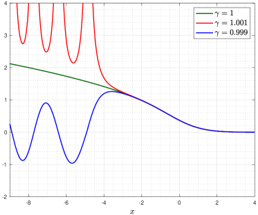
Figure 7. The sensitive dependence of $u=u(x|s)$ for $x\leq 0$ on the monodromy data $s=(-\mathrm{i}\sqrt{\gamma},0,\mathrm{i}\sqrt{\gamma})$ for three values of $\gamma$. In green we show $\gamma=1$, in red $\gamma=1.001$ and in blue $\gamma=0.999$.

For one, the Ablowitz-Segur solution $u=u(x|s)$ is smooth and bounded for $x>0$ and if $x\rightarrow+\infty$, then

$$u(x|s)\sim\sqrt{\gamma}\,\frac{x^{-\frac{1}{4}}}{2\sqrt{\pi}}\mathrm{e}^{-\frac{2}{3}x^{\frac{3}{2}}},$$ (8.2)

which is proportional to the super exponential decay behavior of the Airy function on the positive real axis (recall that (6.12) can be viewed as a nonlinear Airy equation). However, things change dramatically on the half ray $x\leq 0$: if $\gamma\in[0,1)$, then $u(x|s)$ is smooth, bounded and with the following oscillatory behavior as $x\rightarrow-\infty$,

$$u(x|s)\sim(-x)^{-\frac{1}{4}} \,\sqrt{-2\beta}\,\cos\left(\frac{2}{3}(-x)^{\frac{3}{2}}+\beta\ln\big{(}8(-x)^{\frac{3}{2}}\big{)}+\phi\right)$$ (8.3)

$$\,\beta=\frac{1}{2\pi}\ln(1-\gamma),\ \ \ \ \ \phi=\frac{\pi}{4}-\textnormal{arg}\,\Gamma(\mathrm{i}\beta).$$

Expansion (8.3) is due to Ablowitz and Segur [AS1, AS2] and was partially proven in [HM, CM] by Hastings, McLeod and Clarkson, using Gelfand-Levitan type integral equations. The first complete proof of the leading order in (8.3) is due to Its, Kapaev, Suleimanov and Kitaev [IK, Su, Ki] via the isomonodromy method. The first nonlinear steepest descent based proof of (8.3) is in the paper [DZ2] by Deift and Zhou. Next, for $\gamma=1$, the solution $u(x|s)$ is still smooth for $x\leq 0$ but now unbounded, in fact as $x\rightarrow-\infty$

$$u(x|s)\sim\sqrt{-\frac{x}{2}},$$ (8.4)

which, to leading order, can be found in the work of Hastings and McLeod [HM] and to all orders in [DZ2], using once more the nonlinear steepest descent method. Finally, if $\gamma>1$, the qualitative behavior of $u(x|s)$ changes completely: its smoothness is destroyed at finite $x<0$ and solutions blow up, compare the below $x\rightarrow-\infty$ asymptotic expansion,

$$u(x|s)\sim \,\frac{\sqrt{-x}}{\sin(\frac{2}{3}(-x)^{\frac{3}{2}}+\hat{\beta}\ln(8(-x)^{\frac{3}{2}})+\varphi)}$$ (8.5)

$$\,\,\,\,\,\hat{\beta}=\frac{1}{2\pi}\ln(\gamma-1),\ \ \ \ \ \varphi=\frac{\pi}{2}-\textnormal{arg}\,\Gamma\left(\frac{1}{2}+\mathrm{i}\hat{\beta}\right),$$

which is uniform away from the zeros of the trigonometric function appearing in the denominator of (8.5). The singular expansion (8.5) is originally due to Kapaev [Kap] via isomonodromy techniques and was re-derived in [BoI] by nonlinear steepest descent techniques. Note that formulæ (8.2), (8.3), (8.4), (8.5) solve the connection problem for the underlying Painlevé-II transcendent, namely the problem of completely determining the asymptotic behavior of $u(x|s)$ as $x\rightarrow-\infty$, given the same description of $u(x|s)$ as $x\rightarrow+\infty$, or vice versa. Such connection problems are standard exercises in classical special function theory and commonly solved based on contour integral formulæ. However, the Ablowitz-Segur transcendent $u(x|s)$ does not admit any such explicit formulæ  so it is a great achievement of the Riemann-Hilbert method to be able to solve this genuinely nonlinear connection problem in terms of classical special functions. Even better, one can uniformize the qualitatively different asymptotic behaviors (8.3), (8.4), (8.5) at $x=-\infty$ through the use of Jacobi elliptic functions. This recent breakthrough is contained in the paper [Bo] and was made possible by nonlinear steepest descent techniques.

8.2. The Heisenberg antiferromagnet

We now return to (6.15) and discuss two central results for $P_{n}$ proven in [DIZ, Section $6$]. First, the leading order asymptotic behavior,

$$\ln P_{n}=n^{2}\ln\sin\frac{\phi}{2}+o(n),\ \ \ n\rightarrow\infty,$$

which holds uniformly on compact subsets of $(\frac{\pi}{2},\pi)\ni\phi$. Hence, an overall Gaussian decay of $P_{n}$ with a decay rate that decreases with increasing external magnetic field. Second, the emptiness formation probability (6.15) really depends on two variables, $n$ and $h$, equivalently $n$ and $\xi=\mathrm{e}^{\mathrm{i}\phi}$, compare (6.17). As it turns out $P_{n}$ shares an intimate relation with the Painlevé-VI equation, more precisely $P_{n}$ is the Jimbo-Miwa-Ueno $\tau$-function [JMU, Section $5$] of a particular Painlevé-VI equation when viewed in those variables. Here are the details, see [DIZ, Theorem $6.48$]: Set $t:=\bar{\xi}/\xi$, then

$$t\frac{{\mathrm{d}}}{{\mathrm{d}}t}\ln P_{n}=\frac{t-1}{4y(y-1)(y-t)}\nu^{2}+\frac{n}{2y}\nu;\ \ \ \ \ \ \nu:=(y-1)\frac{(1-n)y+nt}{t-1}-t\frac{{\mathrm{d}}y}{{\mathrm{d}}t},$$

where $y=y(t;n)$ satisfies the Painlevé-VI equation

$$\frac{{\mathrm{d}}^{2}y}{{\mathrm{d}}t^{2}}=\frac{1}{2}\left(\frac{1}{y}+\frac{1}{y-1}+\frac{1}{y-t}\right) \,\left(\frac{{\mathrm{d}}y}{{\mathrm{d}}t}\right)^{2}-\left(\frac{1}{t}+\frac{1}{t-1}+\frac{1}{y-t}\right)\frac{{\mathrm{d}}y}{{\mathrm{d}}t}$$

$$\,\,+\frac{y(y-1)(y-t)}{t^{2}(t-1)^{2}}\left(\frac{1}{2}(n-1)^{2}-\frac{tn^{2}}{2y^{2}}+\frac{t(t-1)}{2(y-t)^{2}}\right).$$

This impressive connection between $P_{n}$ and Painlevé special function theory puts the spin chain model firmly on integrable systems ground and as such should be compared with the famous Jimbo, Miwa 1980 result [JM] on the diagonal Ising correlation functions and their relation to a $\sigma$-version of Painlevé-VI.

8.3. Ulam’s problem

In this section we discuss one of the most beautiful and influential results in mathematical physics that was derived by Riemann-Hilbert techniques over the past 20 years, see [Cor] for a taste of the following discovery’s impact: Choose a permutation $\pi\in S_{n}$. For $1\leq i_{1}<i_{2}<\ldots<i_{k}\leq n$ we say that $(\pi(i_{1}),\ldots,\pi(i_{k}))$ is an increasing subsequence of $\pi$ of length $k$ if

$$\pi(i_{1})<\pi(i_{2})<\ldots<\pi(i_{k}).$$

For instance, if $\pi=(4,2,1,3,5)\in S_{5}$, then $(4,5),(2,3),(2,5),(1,3),(1,5),(3,5)$ are subsequences of length $2$ and $(2,3,5),(1,3,5)$ are subsequences of length $3$. In turn, the maximal length $\ell_{n}(\pi)$ of all increasing subsequences of $\pi$ equals $\ell_{5}(\pi)=3$ in this example. Now randomize the setup and pick $\pi\in S_{n}$ with uniform distribution, i.e. we have

$$\textnormal{Prob}\big{\{}\ell_{n}\leq N\big{\}}=\frac{1}{n!}\,\#\{\pi\in S_{n}:\,\ell_{n}(\pi)\leq N\}.$$

How does $\ell_{n}$ behave statistically for large $n$? This question was raised by Ulam in 1961 [U] and he himself conjectured the first moment convergence

$$\lim_{n\rightarrow\infty}\frac{\mathbb{E}(\ell_{n})}{\sqrt{n}}=c$$ (8.6)

for some constant $c$. Ulam’s problem became known as the problem of rigorously verifying the convergence (8.6) and in turn computing the constant. Many people with different methods contributed to this challenge including Erdős, Hammersley, Logan, Shepp and Vershik, Kerov, ultimately settling on $c=2$, see the recent monograph [BDS, page $3-4$] or [Rom, Section $1.1$] for references. The next statistical quantity of $\ell_{n}$ to be considered was its variance. High precision numerical simulations by Odlyzko in the early 1990s indicated that

$$\lim_{n\rightarrow\infty}\frac{\textnormal{Var}(\ell_{n})}{\sqrt[3]{n}}=c_{0}\approx 0.819\ldots,$$

and from simulations by Odlyzko and Rains

$$\lim_{n\rightarrow\infty}\frac{\mathbb{E}(\ell_{n})-2\sqrt{n}}{\sqrt[6]{n}}=c_{1}\approx-1.758\ldots,$$ (8.7)

which constituted a higher order simulation of $\mathbb{E}(\ell_{n})$ than (8.6). At this point of the story, in 1999, the Riemann-Hilbert/integrable systems community in the form of Baik, Deift and Johansson [BDJ] picked up the loose ends and proved the following spectacular result, settling en route (8.6), (8.7) and then some.

Theorem 8.3 ([BDJ, Theorem $1.1$ and $1.2$]).

Let $u(x|s)$ denote the unique solution of (6.12) with the monodromy data $s=(-\mathrm{i},0,\mathrm{i})$, compare Subsection 8.1. Define the distribution function

$$F(x):=\exp\left[-\int_{x}^{\infty}(y-x)u^{2}(y|s)\,{\mathrm{d}}y\right],\ \ \ x\in\mathbb{R}.$$ (8.8)

Then, for any $x\in\mathbb{R}$,

$$\lim_{n\rightarrow\infty}\textnormal{Prob}\left\{\frac{\ell_{n}-2\sqrt{n}}{\sqrt[6]{n}}\leq x\right\}=F(x)\equiv\textnormal{Prob}\big{\{}\chi\leq x\big{\}},$$

and for any $k\in\mathbb{Z}_{\geq 1}$,

$$\lim_{n\rightarrow\infty}\mathbb{E}(\chi_{n}^{k})=\mathbb{E}(\chi^{k}),\ \ \ \ \ \ \ \chi_{n}:=\frac{\ell_{n}-2\sqrt{n}}{\sqrt[6]{n}}.$$

The distribution function $F(x)$ in (8.8), and it really is a distribution function, see our discussion on the analytic and asymptotic properties of $u(x|s)$ in Subsection 8.1, had appeared a few years prior to the Baik-Deift-Johansson theorem. Namely in the 1994 work of Tracy and Widom [TW] where it was shown to capture the fluctuations of the largest eigenvalue of a matrix drawn from the ensemble (6.21) with quadratic external field, a.k.a. the Gaussian unitary ensemble (GUE), in the large $n$ limit. The appearance of a random matrix theory distribution function in a problem of combinatorics was a big surprise at the time, however it turned out not to be an isolated curiosity. The Tracy-Widom distribution $F(x)$ (8.8) (that name stuck after [BDJ]) has become an ubiquitous limiting distribution that made its way to the financial markets, to wireless communication networks, stochastic growth processes and statistical mechanics, just to name a few areas. See [Q] for an engaging outreach article on the Tracy-Widom law. In fact, twenty years after [BDJ] it has become clear that the Tracy-Widom distribution is a modern day bell curve in that it describes the random fluctuations of a large class of integrable probabilistic models, see Figure 8 for a graph of $F(x)$ and $F^{\prime}(x)$.

Figure 8. Comparing the Tracy-Widom distribution $F(x)$ in red to the standard normal distribution $Z(x)$ in blue. On the left, probability density functions, on the right cumulative distribution functions. The asymmetry of the Tracy-Widom distribution is clearly visible.

The proof of Theorem 8.3 is beyond the material covered in this short note, it is a tour de force journey through (de)-Poissonization arguments, Toeplitz determinants and finally the asymptotic nonlinear steepest descent analysis of orthogonal polynomials on the unit circle. These polynomials can be characterized via a Hilbert boundary value problem in the style of Problem 6.5, we refer the interested reader to the monographs [BDS, Rom].

8.4. Universality in invariant random matrix models

Our last discussion in this section concerns the global and local statistical eigenvalue behavior in the random matrix model (6.21). First, through our assumptions placed on the external field $V:\mathbb{R}\rightarrow\mathbb{R}$, the model’s mean eigenvalue density $\frac{1}{n}K_{n,N}(x,x)$, compare (6.22), has a limit

$$\lim_{\begin{subarray}{c}n,N\rightarrow\infty\\ \frac{n}{N}\rightarrow 1\end{subarray}}\frac{1}{n}K_{n,N}(x,x)=\rho_{V}(x)\geq 0,$$ (8.9)

whose support $\Sigma_{V}:=\overline{\{x\in\mathbb{R}:\,\rho_{V}(x)>0\}}$ is a finite union of intervals. The global limiting behavior (8.9) contains the most basic result in random matrix theory as special case, namely the Wigner semicircular law which asserts the almost sure convergence of the rescaled empirical spectral distribution in the GUE to the limiting distribution with density

$$\rho_{W}(x)=\frac{1}{\pi}\sqrt{(2-x^{2})_{+}}.$$

Figure 9. Wigner’s semicircular law for a rescaled $500\times 500$ GUE matrix on the left. Plotted is the rescaled histogram of its $500$ eigenvalues, sampled $100$ times, against the semicircular density in red. On the right we compare Wigner’s law to the exact eigenvalue density for $n=4$ in blue and to the associated eigenvalue histogram, again sampled $100$ times.

While the limiting density $\rho_{V}$ in (8.9) is determined by the potential $V$, the local eigenvalue statistics are to a large extent independent of $V$ in the large $n,N$ limit. Precisely, and this is the celebrated universality property, the local scaling behavior of $K_{n,N}(x,y)$ is completely determined by the local characteristica of $\rho_{V}$. For instance, in case of (6.21), only two qualitatively different scenarios arise generically, compare Figure 9 for the GUE: if $x^{\ast}\in\Sigma_{V}$ is such that $\rho_{V}(x^{\ast})>0$, then

$$\lim_{n\rightarrow\infty}\frac{1}{n\rho_{V}(x^{\ast})}K_{n,n}\left(x^{\ast}+\frac{\lambda}{n\rho_{V}(x^{\ast})},x^{\ast}+\frac{\mu}{n\rho_{V}(x^{\ast})}\right)=\frac{\sin\pi(\lambda-\mu)}{\pi(\lambda-\mu)}$$ (8.10)

uniformly on compact subsets of $\mathbb{R}\ni\lambda,\mu$. This is the 1996 bulk universality result of Pastur, Shcherbina [PS] which was proven with the resolvent method. Soon after that Bleher, Its [BI] and Deift, Kriecherbauer, McLaughlin, Venakides, Zhou [DKMVZ] fine tuned the Deift-Zhou nonlinear steepest descent method of Section 8 to Problem 6.5 and arrived at the same result. Especially [DKMVZ] has become the standard reference for nonlinear steepest descent techniques used in the asymptotic analysis of orthogonal polynomials, and it has been extended in various directions. Those directions lead in turn to generalizations of the bulk universality class (8.10) and extensions to other types of orthogonal polynomial random matrix models, see Section 10 below for a few references. The second case concerns the scaling limit of $K_{n,n}(x,y)$ at a boundary point $x^{\ast}\in\partial\Sigma_{V}$ where $\rho_{V}$ typically vanishes square root like, certainly in the GUE. In this case (8.10) is replaced by the limit

$$\lim_{n\rightarrow\infty}\frac{1}{(cn)^{\frac{2}{3}}}K_{n,n}\left(x^{\ast}+\frac{\lambda}{(cn)^{\frac{2}{3}}},x^{\ast}+\frac{\mu}{(cn)^{\frac{2}{3}}}\right)=\frac{\textnormal{Ai}(\lambda)\textnormal{Ai}^{\prime}(\mu)-\textnormal{Ai}^{\prime}(\lambda)\textnormal{Ai}(\mu)}{\lambda-\mu},$$ (8.11)

if $x^{\ast}$ is a right boundary point and with a sign change $(\lambda,\mu)\mapsto(-\lambda,-\mu)$ in the left hand side of (8.11) for a left boundary point. The limit is again uniform on compact subsets of $\mathbb{R}\ni\lambda,\mu$, it is expressed in terms of the Airy function $w=\textnormal{Ai}(z)$ and $c>0$ denotes some constant. The first proof of the soft edge universality (8.11) is due to Deift, Kriecherbauer, McLaughlin, Venakides, Zhou [DKMVZ] and in more explicit form due to Deift, Gioev [DG], in both cases based on nonlinear steepest descent techniques.

In summary of this short subsection, the earliest universality results in random matrix theory were almost exclusively derived with Riemann-Hilbert nonlinear steepest descent techniques and thus paved the way for subsequent discoveries. Nowadays a wide array of different techniques is available in the derivation of RMT universality classes, some more suitable to certain ensembles than others. Most recently, the work of Erdős and Yau [EY] put forth a toolbox useful in the universality analysis of Wigner random matrices, a broader class of symmetric matrices with independent entries. It is an open question whether the Wigner ensemble is accessible via Riemann-Hilbert techniques.

9. One more example

In this section we will venture into the world of operator-valued Hilbert boundary value problems, a topic which has received far less attention so far, especially from a mathematically rigorous perspective. The only exception is the work of Its, Kozlowski [IKo] and to a certain extent the paper [IS] by Its, Slavnov which we will discuss towards the end. Here is our motivation to think about such problems: consider the stochastic heat equation (SHE)

$$\mathcal{Z}_{T}=\frac{1}{2}\mathcal{Z}_{XX}-\mathcal{Z}\dot{\mathscr{W}},\ \ \ \ \ \ \ \ \mathcal{Z}=\mathcal{Z}(X,T):\mathbb{R}\times(0,\infty)\rightarrow\mathbb{R}$$

with distributional initial data $\mathcal{Z}(X,0)=\delta(X)$ and a Gaussian white noise $\dot{\mathscr{W}}=\dot{\mathscr{W}}(X,T)$. Using the Hopf-Cole transformation $\mathcal{H}(X,T):=-\ln\mathcal{Z}(X,T)$ the SHE is mapped to the celebrated Kardar-Parisi-Zhang (KPZ) equation

$$\mathcal{H}_{T}=\frac{1}{2}\mathcal{H}_{ZZ}-\frac{1}{2}(\mathcal{H}_{Z})^{2}+\dot{\mathscr{W}}$$ (9.1)

which has become the quintessential model for random surface growth processes with several remarkable connections to a number of different physical phenomena, see [Cor0] for a detailed summary. One of the long-standing goals in the analysis of the KPZ equation was achieved in 2011 when Amir, Corwin and Quastel [ACQ] derived the exact probability distribution of its solution with narrow wedge initial data. This allowed in turn to finally verify the celebrated KPZ scaling hypothesis for the KPZ equation itself. Here are the relevant details:

Theorem 9.1 ([ACQ, Theorem $1.1$]).

For any $X\in\mathbb{R}$ and $T>0$ the Hopf-Cole solution $\mathcal{H}(X,T)=-\ln\mathcal{Z}(X,T)$ to the KPZ equation (9.1) with initial data $\mathcal{Z}(X,0)=\delta(X)$ has the probability distribution

$$F_{T}(s):=\textnormal{Prob}\bigg{\{}\mathcal{H}(X,T)-\frac{X^{2}}{2T}-\frac{T}{24}\geq-s\bigg{\}},\ \ s\in\mathbb{R},$$

which is independent of $X\in\mathbb{R}$ and which equals

$$F_{T}(s)=\int_{\Gamma}\det\big{(}1-K_{\sigma_{T,z}}\upharpoonright_{L^{2}(\kappa_{T}^{-1}s,\infty)}\big{)}\mathrm{e}^{-z}\frac{{\mathrm{d}}z}{z}.$$ (9.2)

In (9.2) we choose a Hankel contour $\Gamma$ around $\mathbb{R}_{\geq 0}$, we abbreviate $\kappa_{T}:=(T/2)^{1/3}$ and $K_{\sigma}$ is the integral operator with kernel

$$K_{\sigma}(x,y):=\int_{-\infty}^{\infty}\sigma(t)\textnormal{Ai}(x+t)\textnormal{Ai}(y+t)\,{\mathrm{d}}t\ \ \ \ \ \ \textnormal{and}\ \ \ \ \ \ \sigma_{T,z}(t):=\frac{z}{z-\mathrm{e}^{-\kappa_{T}t}}.$$

The explicit formula (9.2) makes it possible to analyze the statistics of the KPZ equation in the two extreme cases $T\downarrow 0$ and $T\rightarrow\infty$. First, under the KPZ scaling $T^{1/3}$, the statistics converges to the Tracy-Widom distribution (8.8) for large $T$, cf. [ACQ, Corollary $1.3$],

$$\lim_{T\rightarrow\infty}F_{T}\big{(}(T/2)^{1/3}x\big{)}=F(x),\ \ \ \ \ x\in\mathbb{R}.$$ (9.3)

Second, under the scaling $T^{1/4}$, the statistics converges to the standard normal distribution for small $T$, cf. [ACQ, Proposition $1.8$],

$$\lim_{T\downarrow 0}F_{T}\big{(}2^{-1/2}(\pi T)^{1/4}(x-\ln\sqrt{2\pi T})\big{)}=Z(x),\ \ \ \ \ \ x\in\mathbb{R}.$$ (9.4)

Hence, the KPZ equation interpolates between two universality classes and (9.2) is therefore a crossover distribution.

From a Riemann-Hilbert/integrable systems viewpoint we are interested in the Fredholm determinant entering the Amir-Corwin-Quastel formula (9.2). Integrating by parts we can rewrite its kernel in the form

$$(x-y)K_{\sigma}(x,y)=\int_{-\infty}^{\infty}\big{(}\textnormal{Ai}(x+t)\textnormal{Ai}^{\prime}(y+t)-\textnormal{Ai}^{\prime}(x+t)\textnormal{Ai}(y+t)\big{)}{\mathrm{d}}\sigma(t)$$ (9.5)

with the measure ${\mathrm{d}}\sigma(t):=\sigma^{\prime}(t)\,{\mathrm{d}}t$. Besides the particular choice of $\sigma=\sigma_{T,z}$ in (9.2), equality in (9.5) holds as soon as $\sigma:\mathbb{R}\rightarrow\mathbb{C}$ is smooth and

$$\lim_{t\rightarrow-\infty}\sigma(t)=0,\ \ \ \ \ \ \ \ \ \ \ \ \lim_{t\rightarrow+\infty}\sigma(t)=1\ \ \ \ \textnormal{exponentially fast}.$$

Note that (9.5) includes the Fermi factor choice

$$\sigma(t)=\frac{1}{1+\mathrm{e}^{-\alpha t}},\,\,\,\alpha>0,$$

which plays an important role in the analysis of the Moshe-Neuberger-Shapiro random matrix ensemble [Joh, $(14)$], [LW, $(23)$] and in the analysis of non-interacting quantum many-body systems [DMS, $(158)$]. Now given the formal - think of $\sigma(t)=\chi_{[0,\infty)}(t)$ - similarities between (9.5) and the standard Airy kernel (8.11) one might ask for an analogue of the Tracy-Widom Painlevé-II formula (8.8) for the Fredholm determinant of (9.5) on $L^{2}(s,\infty)$, perhaps even an underlying Lax pair which would further strengthen the connection between Theorem 9.1 and integrable systems theory. The task of finding an analogue of (8.8) has been completed in [ACQ, Section $5$] using the techniques of [TW], see Theorem 9.21 below. Here, we will employ Riemann-Hilbert methods and en route reproduce the Amir-Corwin-Quastel formula [ACQ, Proposition $5.2$] while identifying an underlying Lax pair. Our approach is motivated by the duality between the kernels involved, namely

$$K_{\textnormal{Ai}}(x,y)=\frac{\sum_{i=1}^{n}f_{i}(x)g_{i}(y)}{x-y}\ \ \ \ \ \ \ \leftrightarrow\ \ \ \ \ \ \ K_{\sigma}(x,y)=\frac{\int f(x,t)g(y,t){\mathrm{d}}\sigma(t)}{x-y},$$

i.e. the matrix-valued methods of Subsection 6.4 will be lifted to operator-valued ones.

9.1. Technicalities up front

Throughout we are considering kernels $K_{\sigma}$ of the form (9.5) where ${\mathrm{d}}\sigma$ is a positive Borel probability measure on $\mathbb{R}$ for which all moments are finite, i.e.

$$\int_{\mathbb{R}}|t|^{k}{\mathrm{d}}\sigma(t)<\infty,\ \ \ k\in\mathbb{Z}_{\geq 0},$$

and which is absolutely continuous with respect to the Lebesgue measure.

Definition 9.2.

Let $p\in\mathbb{Z}_{\geq 1}$. We require the following abbreviations:

1. The direct sum Hilbert space

   $$\mathcal{H}_{p}:=\bigoplus_{j=1}^{p}L^{2}(\mathbb{R},{\mathrm{d}}\sigma)=\Big{\{}f=(f_{1},\ldots,f_{p})^{\top}\in\mathbb{C}^{p\times 1}:\,f_{j}\in L^{2}(\mathbb{R},{\mathrm{d}}\sigma)\Big{\}},$$

   equipped with the standard inner product $\langle f,g\rangle_{\mathcal{H}_{p}}:=\sum_{j=1}^{p}\int_{\mathbb{R}}f_{j}(t)\overline{g_{j}(t)}{\mathrm{d}}\sigma(t)$ and induced norm $\|f\|_{\mathcal{H}_{p}}:=\sqrt{\langle f,f\rangle_{\mathcal{H}_{p}}}$.

2. The space $L^{2}(\mathbb{R},{\mathrm{d}}\sigma;\mathbb{C}^{p\times p})$ of $p\times p$ matrix-valued functions with entries in $L^{2}(\mathbb{R},{\mathrm{d}}\sigma)$, equipped with the norm

   $$\|X\|_{L^{2}(\mathbb{R},{\mathrm{d}}\sigma;\mathbb{C}^{p\times p})}:=\left[\int_{\mathbb{R}}\textnormal{tr}\big{(}X(t)X^{\dagger}(t)\big{)}{\mathrm{d}}\sigma(t)\right]^{1/2},\ \ \ \ X=\big{[}X^{ij}\big{]}_{i,j=1}^{p}.$$

3. The space $\mathcal{I}(\mathcal{H}_{p})$ of Hilbert-Schmidt integral operators on $\mathcal{H}_{p}$ of the form

   $$\big{(}Kf\big{)}(x)=\int_{\mathbb{R}}K(x,y)f(y)\,{\mathrm{d}}\sigma(y),$$

   with kernel $K\in L^{2}(\mathbb{R}^{2},{\mathrm{d}}\sigma\otimes{\mathrm{d}}\sigma;\mathbb{C}^{p\times p})$.

4. The matrix identity operator $\mathbb{I}_{p}$ on $\mathcal{H}_{p}$.

Next, fix some region $\Omega\subset\mathbb{C}$ and consider $K=K(z)\in\mathcal{I}(\mathcal{H}_{p})$ which depends on an auxiliary variable $z\in\Omega$. We now define the notion of an analytic integral operator, cf. [IKo, page $1781$].

Definition 9.3.

We say that $K(z)\in\mathcal{I}(\mathcal{H}_{p})$ with kernel $K(z|x,y)$ is analytic in $z\in\Omega$, if

1. for any $(x,y)\in\mathbb{R}^{2}$, the map $z\mapsto K(z|x,y)\in\mathbb{C}^{p\times p}$ is analytic in $\Omega$.

2. for any $z\in\Omega$, the map $(x,y)\mapsto K(z|x,y)$ is in $L^{2}(\mathbb{R}^{2},{\mathrm{d}}\sigma\otimes{\mathrm{d}}\sigma;\mathbb{C}^{p\times p})$.

Furthermore, if $\Sigma\subset\Omega\subset\mathbb{C}$ is an oriented contour which consists of a finite union of smooth oriented curves in $\mathbb{CP}^{1}$ with finitely many self-intersections, we will need boundary values of $K(z)\in\mathcal{I}(\mathcal{H}_{p})$, cf. [IKo, page $1782$].

Definition 9.4.

We say that an analytic in $z\in\Omega\setminus\Sigma$ operator $K(z)\in\mathcal{I}(\mathcal{H}_{p})$ admits continuous boundary values $K_{\pm}(z)\in\mathcal{I}(\mathcal{H}_{p})$ on $\Sigma^{\prime}\subset\Sigma$ with kernels $K_{\pm}(z|x,y)$ if

1. for any $(x,y)\in\mathbb{R}^{2}$, the map $z\mapsto K_{\pm}(z|x,y)\in\mathbb{C}^{p\times p}$ is continuous on $\Sigma^{\prime}$.

2. for any $(x,y)\in\mathbb{R}^{2}$, the non-tangental limits

   $$\lim_{\lambda\rightarrow z}K(\lambda|x,y)=K_{\pm}(z|x,y),\ \ \ \ \lambda\in\,\pm\,\textnormal{side of}\,\,\Sigma^{\prime}\ \textnormal{at}\,z$$

   exist.

At this point we record two basic results about the kernel (9.5).

Lemma 9.5.

Let $K_{\sigma}:L^{2}(s,\infty)\rightarrow L^{2}(s,\infty)$ be given by

$$(K_{\sigma}f)(x):=\int_{s}^{\infty}K_{\sigma}(x,y)f(y)\,{\mathrm{d}}y,$$ (9.6)

in terms of the kernel (9.5). Then $K_{\sigma}$ is trace class for any $s\in\mathbb{R}$.

Proof.

If $\sigma(t)$ is the aforementioned Fermi factor, then the claim is proven in [Joh, Proposition $1.1$]. For general $\sigma$ we argue as follows: write

$$K_{\sigma}(x,y)=\int_{-\infty}^{\infty}\left[\int_{0}^{\infty}\textnormal{Ai}(x+t+u)\textnormal{Ai}(y+t+u)\,{\mathrm{d}}u\right]{\mathrm{d}}\sigma(t),$$

and obtain that for any $x_{1},\ldots,x_{n}\in(s,\infty)$ and $z_{1},\ldots,z_{n}\in\mathbb{C}$,

$$\sum_{i,j=1}^{n}z_{i}\overline{z_{j}}K_{\sigma}(x_{i},x_{j})=\int_{-\infty}^{\infty}\bigg{[}\int_{0}^{\infty}\bigg{|}\sum_{i=1}^{n}z_{i}\textnormal{Ai}(x_{i}+t+u)\bigg{|}^{2}{\mathrm{d}}u\bigg{]}{\mathrm{d}}\sigma(t)\geq 0.$$

Thus, with $K_{\sigma}(x,y)=K_{\sigma}(y,x)$, the function $K_{\sigma}(x,y)$ is Hermitian positive definite, so the claim follows provided we can show that

$$\int_{s}^{\infty}K_{\sigma}(x,x)\,{\mathrm{d}}x<\infty,$$ (9.7)

see [Sim, Theorem $2.12$]. In order to get to (9.7) we compute the elementary integral,

$$\int_{s}^{\infty}\textnormal{Ai}^{2}(x+u)\,{\mathrm{d}}u=\big{(}\textnormal{Ai}^{\prime}(x+s)\big{)}^{2}-(x+s)\textnormal{Ai}^{2}(x+s),\ \ \ \ x\in\mathbb{R},$$

apply Fubini’s theorem,

$$\int_{s}^{\infty}K_{\sigma}(x,x)\,{\mathrm{d}}x=\int_{-\infty}^{\infty}\left[\int_{s+t}^{\infty}\Big{\{}\big{(}\textnormal{Ai}^{\prime}(x)\big{)}^{2}-x\textnormal{Ai}^{2}(x)\Big{\}}{\mathrm{d}}x\right]{\mathrm{d}}\sigma(t),$$

and estimate for any $y\in\mathbb{R}$, cf. [NIST, $\S 9.7$],

$$\int_{y}^{\infty}\Big{|}\big{(}\textnormal{Ai}^{\prime}(x)\big{)}^{2}-x\textnormal{Ai}^{2}(x)\Big{|}{\mathrm{d}}x\leq c|y|^{\frac{3}{2}},\ \ \ c>0.$$

Hence (9.7) follows from our finite moment assumption placed on the Borel measure ${\mathrm{d}}\sigma$. ∎

Next to the trace class property of $K_{\sigma}$ we will also need the following result which is well-known at least for the Airy operator induced by the kernel (8.11), i.e. for $\sigma(t)=\chi_{[0,\infty)}(t)$ in (9.5).

Proposition 9.6.

For every $s\in\mathbb{R}$, the self-adjoint operator $K_{\sigma}$ on $L^{2}(s,\infty)$ satisfies $0\leq K_{\sigma}\leq 1$. Moreover, $1-K_{\sigma}$ is invertible on $L^{2}(s,\infty)$.

Proof.

We employ the standard Fourier transform trick, cf. [BDS, Lemma $6.15$], and therefore use

$$\textnormal{Ai}(x)=\frac{1}{2\pi}\int_{-\infty}^{\infty}\mathrm{e}^{\mathrm{i}(\frac{1}{3}y^{3}+xy)}\,{\mathrm{d}}y,\ \ \ \ x\in\mathbb{R}.$$

First compute for any $f\in L^{2}(s,\infty)$,

$$\langle f,K_{\sigma}f\rangle_{L^{2}(s,\infty)}=\int_{-\infty}^{\infty}\bigg{[}\int_{t}^{\infty}\left|\int_{-\infty}^{\infty}\textnormal{Ai}(x+u)f_{s}(x)\,{\mathrm{d}}x\right|^{2}{\mathrm{d}}u\bigg{]}{\mathrm{d}}\sigma(t)\geq 0,$$ (9.8)

with $f_{s}(x):=f(x)\chi_{(s,\infty)}(x)$ using the characteristic function of $(s,\infty)\subset\mathbb{R}$. But from the Fourier representation, for any $u\in\mathbb{R}$,

$$\int_{-\infty}^{\infty}\textnormal{Ai}(x+u)f_{s}(x)\,{\mathrm{d}}x=\frac{1}{\sqrt{2\pi}}\int_{-\infty}^{\infty}\mathrm{e}^{\mathrm{i}(\frac{1}{3}y^{3}+uy)}\check{f}_{s}(-y)\,{\mathrm{d}}y=\check{g}(-u),$$

where $\check{f}_{s}(y):=\frac{1}{\sqrt{2\pi}}\int_{-\infty}^{\infty}f_{s}(x)\mathrm{e}^{-\mathrm{i}xy}{\mathrm{d}}x$ and we set $g(y):=\mathrm{e}^{\frac{\mathrm{i}}{3}y^{3}}\check{f}_{s}(-y)$. Hence, back in (9.8), we find

$$0\leq\langle f,K_{\sigma}f\rangle_{L^{2}(s,\infty)}=\int_{-\infty}^{\infty}\bigg{[}\int_{t}^{\infty}|\check{g}(-u)|^{2}\,{\mathrm{d}}u\bigg{]}{\mathrm{d}}\sigma(t)\leq\int_{-\infty}^{\infty}\bigg{[}\int_{-\infty}^{\infty}|\check{g}(-u)|^{2}\,{\mathrm{d}}u\bigg{]}{\mathrm{d}}\sigma(t)$$

and thus, since ${\mathrm{d}}\sigma$ is a probability measure,

$$0\leq\langle f,K_{\sigma}f\rangle_{L^{2}(s,\infty)}\leq\int_{-\infty}^{\infty}|\check{g}(-u)|^{2}\,{\mathrm{d}}u=\int_{-\infty}^{\infty}|g(u)|^{2}\,{\mathrm{d}}u=\int_{-\infty}^{\infty}|f_{s}(y)|^{2}\,{\mathrm{d}}y=\langle f,f\rangle_{L^{2}(s,\infty)},$$

where we used Plancherel’s theorem in the first and second equality. This shows all together that $0\leq K_{\sigma}\leq 1$ and so, by self-adjointness, also $\|K_{\sigma}\|\leq 1$ in operator norm. Finally, since $K_{\sigma}$ is compact, it is sufficient to establish that $1-K_{\sigma}$ is injective in order to conclude that $1-K_{\sigma}$ is invertible on $L^{2}(s,\infty)$. So assume there is $f\in L^{2}(s,\infty)\setminus\{0\}$ such that $K_{\sigma}f=f$. Then all inequalities above must be equalities for this $f$, i.e. in particular

$$\langle f,K_{\sigma}f\rangle=\int_{-\infty}^{\infty}\bigg{[}\int_{t}^{\infty}|\check{g}(-u)|^{2}\,{\mathrm{d}}u\bigg{]}{\mathrm{d}}\sigma(t)=\int_{-\infty}^{\infty}|\check{g}(-u)|^{2}\,{\mathrm{d}}u,$$

and which implies that

$$\int_{-\infty}^{\infty}\bigg{[}\int_{-\infty}^{t}|\check{g}(-u)|^{2}\,{\mathrm{d}}u\bigg{]}{\mathrm{d}}\sigma(t)=0.$$

But ${\mathrm{d}}\sigma$ is a positive Borel probability measure which is absolutely continuous with respect to the Lebesgue measure, so we must have

$$\sigma\textnormal{-}\textnormal{a.e.}:\ \ \ \int_{-\infty}^{t}|\check{g}(-u)|^{2}\,{\mathrm{d}}u=0\ \ \ \ \ \ \Rightarrow\ \ \ \ \ \ \textnormal{a.e.}:\ \ \ \check{g}(-t)=\int_{s}^{\infty}\textnormal{Ai}(x+t)f(x)\,{\mathrm{d}}x=0,$$

and thus by the analytic properties of the Airy function, $f=0\in L^{2}(s,\infty)$, a contradiction. ∎

We now combine Lemma 9.5 with Proposition 9.6 and conclude that the Fredholm determinant

$$F_{\sigma}(s):=\det\big{(}1-K_{\sigma}\upharpoonright_{L^{2}(s,\infty)}\big{)}=\exp\left[-\sum_{n=1}^{\infty}\frac{1}{n}\mathop{\mathrm{tr}}\limits_{L^{2}(s,\infty)}K_{\sigma}^{n}\right],\ \ \ \ s\in\mathbb{R}$$ (9.9)

is well-defined on one hand and on the other hand satisfies $0<F(s)<1$ for all $s\in\mathbb{R}$. Even better, since

$$\int_{s}^{\infty}\Big{\{}\big{(}\textnormal{Ai}^{\prime}(x)\big{)}^{2}-x\textnormal{Ai}^{2}(x)\Big{\}}{\mathrm{d}}x\,\,>\int_{s^{\prime}}^{\infty}\Big{\{}\big{(}\textnormal{Ai}^{\prime}(x)\big{)}^{2}-x\textnormal{Ai}^{2}(x)\Big{\}}{\mathrm{d}}x$$

whenever $s<s^{\prime}$, we also have that $F_{\sigma}(s)$ is strictly increasing in $s$, so $F_{\sigma}(s)$ is a distribution function of some random variable (one also needs Deift’s Lemma [ACQ, Lemma $2.20$] for the regularity of $F_{\sigma}(s)$ in $s$). Additionally, see [Sosh, Theorem $3$], there is a determinantal process with correlation kernel $K_{\sigma}$. These features of (9.9) and (9.5) are not surprising in light of Johansson’s discussion of the interpolating process in [Joh, Section $1.4$]. However we emphasize that [Joh] uses the Fermi factor choice for $\sigma$, here we are in a more general setup.

9.2. Solvability of the operator-valued problem

We now proceed to characterize (9.9) through a naturally associated Hilbert boundary value problem - very much as in Subsection 6.4, but the problem is going to be operator-valued from the start. First, write

$$F_{\sigma}(s)=\det\big{(}1-K_{\sigma,s}\upharpoonright_{L^{2}(0,\infty)}\big{)},$$

where $K_{\sigma,s}$ has kernel $K_{\sigma,s}(x,y):=K_{\sigma}(x+s,y+s)$. Then consider the following operators (we suppress the explicit $s$-dependence in our notation).

Definition 9.7.

Let $M_{i}(z)\otimes K_{j}(z)\in\mathcal{I}(\mathcal{H}_{1}),i.j=1,2$ denote the $(0,\infty)\ni z$-parametric family of rank one integral operators with kernels

$$\big{(}M_{i}(z)\otimes K_{j}(z)\big{)}(x,y):=m_{i}(z|x)k_{j}(z|y),\ \ \ \ x,y\in\mathbb{R},$$

defined in terms of the $(0,\infty)\ni z$-parametric family of functions

$$m_{1}(z|x)=k_{2}(z|x):=\textnormal{Ai}^{\prime}(z+s+x),\ \ \ \ \ \ \ m_{2}(z|x)=k_{1}(z|x):=\textnormal{Ai}(z+s+x).$$ (9.10)

Equivalently, $M_{i}(z)$ are the operators on $\mathcal{H}_{1}$ which multiply by the functions $m_{i}(z|x)$,

$$\big{(}M_{i}(z)f\big{)}(x):=m_{i}(z|x)f(x),$$

and $K_{j}(z)$ are the integral operators on $\mathcal{H}_{1}$ with kernel $k_{j}(z|y)$,

$$\big{(}K_{j}(z)f\big{)}(x):=\int_{-\infty}^{\infty}k_{j}(z|y)f(y)\,{\mathrm{d}}\sigma(y).$$

Here is the relevant operator-valued Hilbert boundary value problem.

Hilbert Boundary Value Problem 9.8.

For any $s\in\mathbb{R}$, determine $X(z)=X(z;s)\in\mathcal{I}(\mathcal{H}_{2})$ such that

1. $X(z)=\mathbb{I}_{2}+X_{0}(z)$ and $X_{0}(z)\in\mathcal{I}(\mathcal{H}_{2})$ with kernel $X_{0}(z|x,y)$ is analytic in $\mathbb{C}\setminus[0,\infty)$.

2. $X(z)$ admits continuous boundary values $X_{\pm}(z)\in\mathcal{I}(\mathcal{H}_{2})$ on $(0,\infty)\subset\mathbb{R}$, oriented from $-\infty$ to $+\infty$, which satisfy $X_{+}(z)=X_{-}(z)G(z)$ with

   $$G(z)=\mathbb{I}_{2}+2\pi\mathrm{i}\begin{bmatrix}M_{1}(z)\otimes K_{1}(z)&-M_{1}(z)\otimes K_{2}(z)\vskip 3.0pt plus 1.0pt minus 1.0pt\\ M_{2}(z)\otimes K_{1}(z)&-M_{2}(z)\otimes K_{2}(z)\end{bmatrix}.$$ (9.11)

3. There exist operators $F_{i}$ on $\mathcal{H}_{1}$ which multiply by $z$-independent functions $f_{i}\in L^{1}(\mathbb{R},{\mathrm{d}}\sigma)\cap L^{\infty}(\mathbb{R},{\mathrm{d}}\sigma)$ such that for $|z|<\epsilon$, in terms of any branch for $\ln:\mathbb{C}\setminus[0,\infty)\rightarrow\mathbb{C}$,

   $$X(z)=\mathbb{I}_{2}-\begin{bmatrix}F_{1}\otimes K_{1}(0)&-F_{1}\otimes K_{2}(0)\vskip 3.0pt plus 1.0pt minus 1.0pt\\ F_{2}\otimes K_{1}(0)&-F_{2}\otimes K_{2}(0)\end{bmatrix}\ln z+X_{\textnormal{reg}}(z),$$ (9.12)

   where $X_{\textnormal{reg}}(z)\in\mathcal{I}(\mathcal{H}_{2})$ with kernel $X_{\textnormal{reg}}(z|x,y)$ is analytic at $z=0$ and satisfies

   $$\|X_{\textnormal{reg}}(z|x,y)\|\leq c|1+s+x|^{\frac{3}{4}}|1+s+y|^{\frac{3}{4}}\ \ \ \textnormal{as}\ \ z\rightarrow 0$$ (9.13)

   for all $(x,y)\in\mathbb{R}^{2}$ with $c>0$.

4. For any compact subset $V\subset\mathbb{C}$ with $\textnormal{dist}(0,V)>0$ there exists $c=c(V)>0$ such that for $z\in\mathbb{C}\setminus V$,

   $$\|X_{0}(z|x,y)\|\leq\frac{c}{1+|z|}|s+x|^{\frac{3}{4}}|s+y|^{\frac{3}{4}}$$ (9.14)

   uniformly in $(x,y)\in\mathbb{R}^{2}$.

Our first result concerns the unique solvability of Problem 9.8

Theorem 9.9.

The Hilbert boundary value problem 9.8 is uniquely solvable for any $s\in\mathbb{R}$ and its solution takes the form

$$X(z)=\mathbb{I}_{2}+\int_{0}^{\infty}\begin{bmatrix}N_{1}(w)\otimes K_{1}(w)&-N_{1}(w)\otimes K_{2}(w)\vskip 3.0pt plus 1.0pt minus 1.0pt\\ N_{2}(w)\otimes K_{1}(w)&-N_{2}(w)\otimes K_{2}(w)\end{bmatrix}\frac{{\mathrm{d}}w}{w-z},\ \ \ z\in\mathbb{C}\setminus[0,\infty),$$ (9.15)

where $N_{i}(w)$ are the operators on $\mathcal{H}_{1}$ which multiply by the functions $n_{i}(w|x)$ determined from the integral equation

$$(1-K_{\sigma,s}\upharpoonright_{L^{2}(0,\infty)})n_{i}(\cdot|x)=m_{i}(\cdot|x),\ \ \ i=1,2,$$ (9.16)

with $x\in\mathbb{R}$.

Proof.

Suppose first that Problem 9.8 is solvable. By condition (1), estimate (9.14) and the moment assumption on ${\mathrm{d}}\sigma$, the Fredholm determinant

$$e(z):=\det\big{(}\mathbb{I}_{2}+X_{0}(z)\upharpoonright_{\mathcal{H}_{2}}\big{)},\ \ \ z\in\mathbb{C}\setminus[0,\infty)$$

is well-defined in the indicated $z$-domain by Hadamard’s inequality (by condition (1) only, $X_{0}(z)$ is a Hilbert-Schmidt operator, but (4) ensures that the ordinary Fredholm determinant on $\mathcal{H}_{2}$ converges). Moreover, by Morera’s and Fubini’s theorem, analyticity of $X_{0}(z)$ in $\mathbb{C}\setminus[0,\infty)$ implies analyticity of $e(z)$ in $\mathbb{C}\setminus[0,\infty)$. Furthermore, using (9.14) again and the dominated convergence theorem, the boundary values $e_{\pm}(z),z\in(0,\infty)$ satisfy

$$e_{\pm}(z)=\det\big{(}X_{\pm}\upharpoonright_{\mathcal{H}_{2}}\big{)},\ \ \ z\in(0,\infty).$$ (9.17)

Our immediate goal is to derive a scalar Hilbert boundary value problem for $e(z)$: from condition (2) we have $G(z)=\mathbb{I}_{2}+G_{0}(z)$ where $G_{0}(z)\in\mathcal{I}(\mathcal{H}_{2})$ is trace class on $\mathcal{H}_{2}$ and satisfies the estimate, compare Definition 9.7 and [NIST, $\S 9.7$],

$$\|G_{0}(z|x,y)\|\leq c|z+s+x|^{\frac{1}{4}}|z+s+y|^{\frac{1}{4}},\ \ \ \ c>0,$$

uniformly in $(z,x,y)\in\mathbb{R}^{3}$. This ensures existence of the determinant $\det(\mathbb{I}_{2}+G_{0}(z)\upharpoonright_{\mathcal{H}_{2}})$ for $z\in\mathbb{R}$ and since

$$\mathop{\mathrm{tr}}\limits_{\mathcal{H}_{2}}G_{0}(z)=0,\ \ \ \ \ \big{(}G_{0}(z)\big{)}^{2}=0,\ \ \ z\in\mathbb{R},$$

we obtain from the Plemelj-Smithies formula [GGK, Chapter II, Theorem $3.1$] that $\det(G(z)\upharpoonright_{\mathcal{H}_{2}})=1$ for all $z\in\mathbb{R}$. With this in hand we return to (9.17), apply condition (2) and the multiplicativity property of Fredholm determinants, in turn

$$e_{+}(z)=e_{-}(z),\ \ z\in(0,\infty).$$

Moreover, estimate (9.14) yields $e(z)\rightarrow 1$ as $z\rightarrow\infty$, so we are left to address the behavior of $e(z)$ in a vicinity of $z=0$. By (9.12) and the estimate (9.13) we see that the operator

$$P(z):=\det\big{(}\mathbb{I}_{2}+X_{\textnormal{reg}}(z)\upharpoonright_{\mathcal{H}_{2}}\big{)}\big{(}\mathbb{I}_{2}+X_{\textnormal{reg}}(z)\big{)}^{-1},\ \ \ |z|<\epsilon$$

on $\mathcal{H}_{2}$ is well-defined even if $\det(\mathbb{I}_{2}+X_{\textnormal{reg}}(z)\upharpoonright_{\mathcal{H}_{2}})$ vanishes at some points in the disk $|z|<\epsilon$, cf. [GGK, Chapter VIII, Theorem $1.1$]. Hence from (9.12), as $z\rightarrow 0$ and $z\notin[0,\infty)$,

$$e(z)=\det\big{(}\mathbb{I}_{2}+X_{\textnormal{reg}}(z)\upharpoonright_{\mathcal{H}_{2}}\big{)}-\big{\langle}P(z)F,K(0)\big{\rangle}_{\mathcal{H}_{2}}\ln z,$$

with $F=[F_{1},F_{2}]^{\top},K(0)=\big{[}K_{1}(0),K_{2}(0)\big{]}^{\top}$. This shows that $|e(z)|\leq c|\ln z|$ when $z\rightarrow 0$ and so all together, $e$ is analytic in $\mathbb{C}\setminus\{0\}$ with a possible blow up at the origin that is logarithmic at worst. Hence, $e(z)$ must be entire and with its limiting behavior at $z=\infty$, thus $e(z)\equiv 1$ for all $z\in\mathbb{C}$. As a consequence of this, we now know that any solution $X(z)\in\mathcal{I}(\mathcal{H}_{2})$ of Problem 9.8 is invertible for all $z\in\mathbb{C}\setminus[0,\infty)$ and so are its continuous boundary values $X_{\pm}(z),z\in(0,\infty)$. Thus, if $X^{(1)}(z),X^{(2)}(z)$ are two solutions of Problem 9.8, then

$$\mathcal{I}(\mathcal{H}_{2})\ni Y(z):=X^{(1)}(z)\big{(}X^{(2)}(z)\big{)}^{-1}=\mathbb{I}_{2}+Y_{0}(z),\ \ \ \ z\in\mathbb{C}\setminus[0,\infty)$$

is analytic in $\mathbb{C}\setminus[0,\infty)$, has continuous boundary values $Y_{\pm}(z)$ on $(0,\infty)$ and it obeys a Problem in the style of Problem 9.8 with

$$Y_{+}(z)=Y_{-}(z),\ \ z\in(0,\infty).$$

Moreover, the kernel $Y_{0}(z|x,y)$ of $Y_{0}(z)$ has at worst a square logarithmic singularity at $z=0$, so the map $z\mapsto Y_{0}(z|x,y)$ is entire $(\sigma\otimes\sigma)$-almost everywhere. But $Y_{0}(z|x,y)\rightarrow 0$ as $z\rightarrow\infty$ also $(\sigma\otimes\sigma)$-almost everywhere, so by Liouville’s theorem we conclude $Y(z)=\mathbb{I}_{2}$ and which proves that Problem 9.8, if solvable, is uniquely solvable.

Second, we prove solvability of Problem 9.8 and recall to this end that $1-K_{\sigma,s}$ is invertible on $L^{2}(0,\infty)$ for any $s\in\mathbb{R}$, see Proposition 9.6. Thus the integral equation (9.16) is uniquely solvable and by the boundedness of the resolvent we find for its solution, uniformly in $x\in\mathbb{R}$,

$$\|n_{i}(\cdot|x)\|_{L^{2}(0,\infty)}\leq c\|m_{i}(\cdot|x)\|_{L^{2}(0,\infty)},\ \ \ \ c>0,\ \ \ i=1,2.$$ (9.18)

Now consider $X(z)$ as in (9.15) and note that the kernel of $X_{0}(z)$ (the integral piece) is built out of the functions

$$X_{0}^{ij}(z|x,y)=\int_{0}^{\infty}n_{i}(w|x)k_{j}(w|y)\frac{{\mathrm{d}}w}{w-z},\ \ \ \ z\notin[0,\infty),\ \ \ (x,y)\in\mathbb{R}^{2}.$$

However, using (9.18) and standard estimates for Airy functions, cf. [NIST, $\S 9.7$] we obtain by Cauchy-Schwarz

$$\big{|}X_{0}^{ij}(z|x,y)\big{|}\leq\frac{c}{\textnormal{dist}(z,\mathbb{R}_{\geq 0})}\,|s+x|^{\frac{3}{4}}|s+y|^{\frac{3}{4}},$$ (9.19)

uniformly in $(x,y)\in\mathbb{R}^{2}$. Thus $(x,y)\mapsto X_{0}(z|x,y)$ is in $L^{2}(\mathbb{R}^{2},{\mathrm{d}}\sigma\otimes{\mathrm{d}}\sigma;\mathbb{C}^{2\times 2})$ for $z\in\mathbb{C}\setminus[0,\infty)$. Moreover, by the standard regularity properties of the resolvent operator, we also find from (9.16) that $z\mapsto X_{0}^{ij}(z|x,y)$ is Hölder continuous on $\mathbb{C}\setminus[0,\infty)$ for any $(x,y)\in\mathbb{R}^{2}$ and $i,j=1,2$. Thus, by the Plemelj-Sokhostki formulæ, $z\mapsto X_{0}(z|x,y)$ is analytic in $\mathbb{C}\setminus[0,\infty)$ for any $(x,y)\in\mathbb{R}^{2}$ and so the right hand side in (9.15) analytic in $z\in\mathbb{C}\setminus[0,\infty)$ according to Definition 9.3. Having just established condition (1) in Problem 9.8, we now turn to (2), (3) and (4): First, estimate (9.14) follows from (9.19) and the Plemelj-Sokhotski formulæ. Second, $z\mapsto X_{0}^{ij}(z|x,y)$ is Hölder continuous on $[0,\infty)$ for any $(x,y)\in\mathbb{R}^{2}$, thus $X(z)$ admits continuous boundary values $X_{\pm}(z)\in\mathcal{I}(\mathcal{H}_{2})$ on $(0,\infty)$ according to Definition 9.4 by the Plemelj-Sokhotski formulæ. Now verify (9.11), so first compute from (9.15),

$$X_{+}(z)-X_{-}(z)=2\pi\mathrm{i}\begin{bmatrix}N_{1}(z)\otimes K_{1}(z)&-N_{1}(z)\otimes K_{2}(z)\vskip 3.0pt plus 1.0pt minus 1.0pt\\ N_{2}(z)\otimes K_{1}(z)&-N_{2}(z)\otimes K_{2}(z)\end{bmatrix},\ \ \ \ \ z\in(0,\infty).$$ (9.20)

On the other hand, by (9.12) and (9.15),

$$X_{-}(z)G(z)= \,X_{-}(z)\left\{\mathbb{I}_{2}+2\pi\mathrm{i}\begin{bmatrix}M_{1}(z)\otimes K_{1}(z)&-M_{1}(z)\otimes K_{2}(z)\vskip 3.0pt plus 1.0pt minus 1.0pt\\ M_{2}(z)\otimes K_{1}(z)&-M_{2}(z)\otimes K_{2}(z)\end{bmatrix}\right\}$$

$$= \,X_{-}(z)+2\pi\mathrm{i}\left\{\mathbb{I}_{2}+\int_{0}^{\infty}\begin{bmatrix}N_{1}(w)\otimes K_{1}(w)&-N_{1}(w)\otimes K_{2}(w)\vskip 3.0pt plus 1.0pt minus 1.0pt\\ N_{2}(w)\otimes K_{1}(w)&-N_{2}(w)\otimes K_{2}(w)\end{bmatrix}\frac{{\mathrm{d}}w}{w-z_{-}}\right\}$$

$$\ \ \ \ \ \ \ \ \ \,\circ\begin{bmatrix}M_{1}(z)\otimes K_{1}(z)&-M_{1}(z)\otimes K_{2}(z)\vskip 3.0pt plus 1.0pt minus 1.0pt\\ M_{2}(z)\otimes K_{1}(z)&-M_{2}(z)\otimes K_{2}(z)\end{bmatrix},\ \ \ \ z\in(0,\infty),$$ (9.21)

and since, using here the general $(N_{i}\otimes K_{j})(M_{j}\otimes K_{\ell})=\langle K_{j},M_{j}\rangle_{\mathcal{H}_{1}}(N_{i}\otimes K_{\ell})$ fact,

$$\begin{bmatrix}N_{1}(w)\otimes K_{1}(w)&-N_{1}(w)\otimes K_{2}(w)\vskip 3.0pt plus 1.0pt minus 1.0pt\\ N_{2}(w)\otimes K_{1}(w)&-N_{2}(w)\otimes K_{2}(w)\end{bmatrix}\begin{bmatrix}M_{1}(z)\otimes K_{1}(z)&-M_{1}(z)\otimes K_{2}(z)\vskip 3.0pt plus 1.0pt minus 1.0pt\\ M_{2}(z)\otimes K_{1}(z)&-M_{2}(z)\otimes K_{2}(z)\end{bmatrix}$$

$$\ \ \ \ \ \ \ \ \,=(w-z)K_{\sigma,s}(w,z)\begin{bmatrix}N_{1}(w)\otimes K_{1}(z)&-N_{1}(w)\otimes K_{2}(z)\vskip 3.0pt plus 1.0pt minus 1.0pt\\ N_{2}(w)\otimes K_{1}(z)&-N_{2}(w)\otimes K_{2}(z)\end{bmatrix},\ \ \ (w,z)\in(0,\infty),\times(0,\infty),$$

the chain of equalities (9.2) simplifies further

$$X_{-}(z)G(z)= \,X_{-}(z)+2\pi\mathrm{i}\begin{bmatrix}M_{1}(z)\otimes K_{1}(z)&-M_{1}(z)\otimes K_{2}(z)\vskip 3.0pt plus 1.0pt minus 1.0pt\\ M_{2}(z)\otimes K_{1}(z)&-M_{2}(z)\otimes K_{2}(z)\end{bmatrix}$$ (9.22)

$$\ \ \ \ \ \ \,+2\pi\mathrm{i}\int_{0}^{\infty}K_{\sigma,s}(w,z)\begin{bmatrix}N_{1}(w)\otimes K_{1}(z)&-N_{1}(w)\otimes K_{2}(z)\vskip 3.0pt plus 1.0pt minus 1.0pt\\ N_{2}(w)\otimes K_{1}(z)&-N_{2}(w)\otimes K_{2}(z)\end{bmatrix}{\mathrm{d}}w,\ \ z\in(0,\infty).$$

But (9.16) is equivalent to the operator equation

$$N_{i}(z)-\int_{0}^{\infty}K_{\sigma,s}(z,w)N_{i}(w)\,{\mathrm{d}}w=M_{i}(z),\ \ \ z\in(0,\infty),$$

which, by symmetry of $K_{\sigma,s}$, simplifies (9.22) to

$$X_{-}(z)G(z)=X_{-}(z)+2\pi\mathrm{i}\begin{bmatrix}N_{1}(z)\otimes K_{1}(z)&-N_{1}(z)\otimes K_{2}(z)\vskip 3.0pt plus 1.0pt minus 1.0pt\\ N_{2}(z)\otimes K_{1}(z)&-N_{2}(z)\otimes K_{2}(z)\end{bmatrix}\stackrel{{\scriptstyle\eqref{SH:18}}}{{=}}X_{+}(z),\ \ \ z\in(0,\infty).$$

Condition (2) in Problem 9.8 has therefore been established and we are left with the singular behavior (9.12) and (9.13) near $z=0$. Fix $z\notin[0,\infty),0<\epsilon<1$ and rewrite (9.15) as

$$X(z) \,=\mathbb{I}_{2}+\ln\left(\frac{z-2\epsilon}{z}\right)\begin{bmatrix}N_{1}(z)\otimes K_{1}(z)&-N_{1}(z)\otimes K_{2}(z)\vskip 3.0pt plus 1.0pt minus 1.0pt\\ N_{2}(z)\otimes K_{1}(z)&-N_{2}(z)\otimes K_{2}(z)\end{bmatrix}$$ (9.23)

$$\,+\int_{0}^{2\epsilon}\left\{\begin{bmatrix}N_{1}(w)\otimes K_{1}(w)&-N_{1}(w)\otimes K_{2}(w)\vskip 3.0pt plus 1.0pt minus 1.0pt\\ N_{2}(w)\otimes K_{1}(w)&-N_{2}(w)\otimes K_{2}(w)\end{bmatrix}-\begin{bmatrix}N_{1}(z)\otimes K_{1}(z)&-N_{1}(z)\otimes K_{2}(z)\vskip 3.0pt plus 1.0pt minus 1.0pt\\ N_{2}(z)\otimes K_{1}(z)&-N_{2}(z)\otimes K_{2}(z)\end{bmatrix}\right\}\frac{{\mathrm{d}}w}{w-z}$$

$$\,+\int_{2\epsilon}^{\infty}\begin{bmatrix}N_{1}(w)\otimes K_{1}(w)&-N_{1}(w)\otimes K_{2}(w)\vskip 3.0pt plus 1.0pt minus 1.0pt\\ N_{2}(w)\otimes K_{1}(w)&-N_{2}(w)\otimes K_{2}(w)\end{bmatrix}\frac{{\mathrm{d}}w}{w-z}.$$

The remaining two integrals are operators in $\mathcal{I}(\mathcal{H}_{2})$ which are analytic in the disk $|z|<\epsilon$ and the same is true for the operator multiplied by the logarithm: indeed we already showed that

$$X_{-}(z)G(z)=X_{-}(z)+2\pi\mathrm{i}\begin{bmatrix}N_{1}(z)\otimes K_{1}(z)&-N_{1}(z)\otimes K_{2}(z)\vskip 3.0pt plus 1.0pt minus 1.0pt\\ N_{2}(z)\otimes K_{1}(z)&-N_{2}(z)\otimes K_{2}(z)\end{bmatrix},\ \ \ z\in(0,\infty),$$ (9.24)

and since the trace class $G(z)\in\mathcal{I}(\mathcal{H}_{2})$ is invertible with

$$\big{(}G(z)\big{)}^{-1}=\mathbb{I}_{2}-2\pi\mathrm{i}\begin{bmatrix}M_{1}(z)\otimes K_{1}(z)&-M_{1}(z)\otimes K_{2}(z)\vskip 3.0pt plus 1.0pt minus 1.0pt\\ M_{2}(z)\otimes K_{1}(z)&-M_{2}(z)\otimes K_{2}(z)\end{bmatrix},\ \ \ z\in\mathbb{R},$$

we also compute (as done previously for $X_{-}(z)G(z)$),

$$X_{+}(z)\big{(}G(z)\big{)}^{-1}= \,X_{+}(z)\left\{\mathbb{I}_{2}-2\pi\mathrm{i}\begin{bmatrix}M_{1}(z)\otimes K_{1}(z)&-M_{1}(z)\otimes K_{2}(z)\vskip 3.0pt plus 1.0pt minus 1.0pt\\ M_{2}(z)\otimes K_{1}(z)&-M_{2}(z)\otimes K_{2}(z)\end{bmatrix}\right\}$$

$$= \,X_{+}(z)-2\pi\mathrm{i}\left\{\mathbb{I}_{2}+\int_{0}^{\infty}\begin{bmatrix}N_{1}(w)\otimes K_{1}(w)&-N_{1}(w)\otimes K_{2}(w)\vskip 3.0pt plus 1.0pt minus 1.0pt\\ N_{2}(w)\otimes K_{1}(w)&-N_{2}(w)\otimes K_{2}(w)\end{bmatrix}\frac{{\mathrm{d}}w}{w-z_{+}}\right\}$$

$$\ \ \ \ \ \ \ \ \ \,\circ\begin{bmatrix}M_{1}(z)\otimes K_{1}(z)&-M_{1}(z)\otimes K_{2}(z)\vskip 3.0pt plus 1.0pt minus 1.0pt\\ M_{2}(z)\otimes K_{1}(z)&-M_{2}(z)\otimes K_{2}(z)\end{bmatrix}$$

$$= \,X_{+}(z)-2\pi\mathrm{i}\begin{bmatrix}N_{1}(z)\otimes K_{1}(z)&-N_{1}(z)\otimes K_{2}(z)\vskip 3.0pt plus 1.0pt minus 1.0pt\\ N_{2}(z)\otimes K_{1}(z)&-N_{2}(z)\otimes K_{2}(z)\end{bmatrix},\ \ z\in(0,\infty).$$ (9.25)

Hence, combining (9.24) and (9.2) with the explicit form (9.11), we deduce

$$X_{\pm}(z)\begin{bmatrix}M_{1}(z)\otimes K_{1}(z)&-M_{1}(z)\otimes K_{2}(z)\vskip 3.0pt plus 1.0pt minus 1.0pt\\ M_{2}(z)\otimes K_{1}(z)&-M_{2}(z)\otimes K_{2}(z)\end{bmatrix}=\begin{bmatrix}N_{1}(z)\otimes K_{1}(z)&-N_{1}(z)\otimes K_{2}(z)\vskip 3.0pt plus 1.0pt minus 1.0pt\\ N_{2}(z)\otimes K_{1}(z)&-N_{2}(z)\otimes K_{2}(z)\end{bmatrix},\ \ z\in(0,\infty),$$

and from this, for $z\in(0,\infty)$, the following operator composition formula for $N_{i}(z)$,

$$N(z)=X(z)M(z);\ \ \ \ \ \ \ N(z):=\big{[}N_{1}(z),N_{2}(z)\big{]}^{\top},\ \ M(z):=\big{[}M_{1}(z),M_{2}(z)\big{]}^{\top},$$ (9.26)

which is independent of the $\pm$ choice for the boundary values of $X(z)$ on $(0,\infty)$. Now use (9.26) back in (9.23) and conclude that $N(z)$ near $z=0$ is of the form

$$N(z)=\big{(}\,\mathbb{I}_{2}+N_{\textnormal{reg}}(z)\big{)}M(z),\ \ \ \ \ \ \ \ \ \ \ \ N_{\textnormal{reg}}(z)\in\mathcal{I}(\mathcal{H}_{2})\ \ \textnormal{is analytic at}\ z=0,$$

since $(N_{i}(z)\otimes K_{1}(z))M_{1}(z)-(N_{i}(z)\otimes K_{2}(z))M_{2}(z)=N_{i}(z)\otimes(M_{1}(z)K_{1}(z)-M_{2}(z)K_{2}(z))=0$, i.e. since the logarithmic term drops out. All together, we can expand $N_{i}(z)$ near $z=0$, which verifies the existence of the multiplication operators $F_{i}$ in (9.12) with their indicated properties, and estimate the kernel

$$\bigg{|} \,\frac{1}{w-z}\left\{\begin{bmatrix}N_{1}(w)\otimes K_{1}(w)&-N_{1}(w)\otimes K_{2}(w)\vskip 3.0pt plus 1.0pt minus 1.0pt\\ N_{2}(w)\otimes K_{1}(w)&-N_{2}(w)\otimes K_{2}(w)\end{bmatrix}-\begin{bmatrix}N_{1}(z)\otimes K_{1}(z)&-N_{1}(z)\otimes K_{2}(z)\vskip 3.0pt plus 1.0pt minus 1.0pt\\ N_{2}(z)\otimes K_{1}(z)&-N_{2}(z)\otimes K_{2}(z)\end{bmatrix}\right\}(x,y)\bigg{|}$$

$$\,\ \ \ \ \ \ \ \ \,\leq c|1+s+x|^{\frac{3}{4}}|1+s+y|^{\frac{3}{4}},\ \ \ c>0,$$

uniformly for $w\in[0,\epsilon]\subset\mathbb{R},|z|<\epsilon$ and any $(x,y)\in\mathbb{R}^{2}$. All combined in (9.23) we have now established (9.12) together with (9.13). This completes our proof. ∎

During our upcoming computations we will use the following consequences of Theorem 9.9.

Corollary 9.10.

Let $X(z)$ denote the unique solution of Problem 9.8. Then

$$\big{(}X(z)\big{)}^{-1}=\mathbb{I}_{2}-\int_{0}^{\infty}\begin{bmatrix}M_{1}(w)\otimes L_{1}(w)&-M_{1}(w)\otimes L_{2}(w)\vskip 3.0pt plus 1.0pt minus 1.0pt\\ M_{2}(w)\otimes L_{1}(w)&-M_{2}(w)\otimes L_{2}(w)\end{bmatrix}\frac{{\mathrm{d}}w}{w-z},\ \ \ z\in\mathbb{C}\setminus[0,\infty),$$ (9.27)

where $L_{i}(w)$ are the integral operators on $\mathcal{H}_{1}$ with kernel $\ell_{i}(z|y)$ determined from the integral equation

$$(1-K_{\sigma,s}\upharpoonright_{L^{2}(0,\infty)})\ell_{i}(\cdot|y)=k_{i}(\cdot|y),\ \ \ i=1,2,$$ (9.28)

with $y\in\mathbb{R}$. Moreover, for any $z\in(0,\infty)$,

$$N(z)=X(z)M(z),\ \ \ \ \ \ \ \ \ \ \ L(z)=K(z)\big{(}X(z)\big{)}^{-1}$$ (9.29)

with $L(z):=\big{[}L_{1}(z),-L_{2}(z)\big{]},K(z):=\big{[}K_{1}(z),-K_{2}(z)\big{]}$ and near $z=0$,

$$N(z)=\big{(}\,\mathbb{I}_{2}+N_{\textnormal{reg}}(z)\big{)}M(z),\ \ \ \ \ \ \ \ \ \ L(z)=K(z)\big{(}\,\mathbb{I}_{2}+L_{\textnormal{reg}}(z)\big{)}$$

where $N_{\textnormal{reg}}(z)\in\mathcal{I}(\mathcal{H}_{2})$ and $L_{\textnormal{reg}}(z)\in\mathcal{I}(\mathcal{H}_{2})$ are analytic at $z=0$.

Proof.

Let $Y(z)$ denote the right hand side of (9.27) and $\overline{Y}_{0}(z)$ the underlying integrand without the Cauchy kernel. With (9.15) we then compute ($\overline{X}_{0}(z)$ being similarly defined)

$$X(z)Y(z)=\mathbb{I}_{2}+\int_{0}^{\infty}\big{(}\overline{X}_{0}(w)-\overline{Y}_{0}(w)\big{)}\frac{{\mathrm{d}}w}{w-z}-\int_{0}^{\infty}\int_{0}^{\infty}\overline{X}_{0}(w)\overline{Y}_{0}(\lambda)\frac{{\mathrm{d}}w}{w-z}\frac{{\mathrm{d}}\lambda}{\lambda-z},\ \ z\notin[0,\infty).$$

But

$$\overline{X}_{0}(w)\overline{Y}_{0}(\lambda)=(w-\lambda)K_{\sigma,s}(w,\lambda)\begin{bmatrix}N_{1}(w)\otimes L_{1}(\lambda)&-N_{1}(w)\otimes L_{2}(\lambda)\vskip 3.0pt plus 1.0pt minus 1.0pt\\ N_{2}(w)\otimes L_{1}(\lambda)&-N_{2}(w)\otimes L_{2}(\lambda)\end{bmatrix},$$

so using partial fractions in the double integral and both integral equations (9.16) and (9.28),

$$\int_{0}^{\infty}\big{(}\overline{X}_{0}(w)-\overline{Y}_{0}(w)\big{)}\frac{{\mathrm{d}}w}{w-z}-\int_{0}^{\infty}\int_{0}^{\infty}\overline{X}_{0}(w)\overline{Y}_{0}(\lambda)\frac{{\mathrm{d}}w}{w-z}\frac{{\mathrm{d}}\lambda}{\lambda-z}=0,\ \ \ z\notin[0,\infty),$$ (9.30)

which shows that $X(z)Y(z)=\mathbb{I}_{2}$ for $z\notin[0,\infty)$. But any solution $X(z)\in\mathcal{I}(\mathcal{H}_{2})$ of Problem 9.8 is invertible, so a one-sided inverse is a two-sided inverse and thus identity (9.27) holds for $z\notin[0,\infty)$. Moving ahead, the first half of (9.29) and the associated local regularity statement have already been proven above. Focusing thus on the second half, the right hand side in (9.27) is such that by the Plemelj-Sokhotski formula

$$\big{(}X(z)\big{)}^{-1}_{+}-\big{(}X(z)\big{)}^{-1}_{-}=-2\pi\mathrm{i}\begin{bmatrix}M_{1}(z)\otimes L_{1}(z)&-M_{1}(z)\otimes L_{2}(z)\vskip 3.0pt plus 1.0pt minus 1.0pt\\ M_{2}(z)\otimes L_{1}(z)&-M_{2}(z)\otimes L_{2}(z)\end{bmatrix},\ \ \ z\in(0,\infty),$$ (9.31)

as well as

$$\big{(}G(z)\big{)}^{-1}\big{(}X(z)\big{)}^{-1}_{-}= \,\left\{\mathbb{I}_{2}-2\pi\mathrm{i}\begin{bmatrix}M_{1}(z)\otimes K_{1}(z)&-M_{1}(z)\otimes K_{2}(z)\vskip 3.0pt plus 1.0pt minus 1.0pt\\ M_{2}(z)\otimes K_{1}(z)&-M_{2}(z)\otimes K_{2}(z)\end{bmatrix}\right\}\big{(}X(z)\big{)}^{-1}_{-}$$

$$\stackrel{{\scriptstyle\eqref{SH:24}}}{{=}} \,\big{(}X(z)\big{)}^{-1}_{-}-2\pi\mathrm{i}\begin{bmatrix}M_{1}(z)\otimes K_{1}(z)&-M_{1}(z)\otimes K_{2}(z)\vskip 3.0pt plus 1.0pt minus 1.0pt\\ M_{2}(z)\otimes K_{1}(z)&-M_{2}(z)\otimes K_{2}(z)\end{bmatrix}$$

$$\ \ \ \ \ \ \ \ \circ\left\{\mathbb{I}_{2}-\int_{0}^{\infty}\begin{bmatrix}M_{1}(w)\otimes L_{1}(w)&-M_{1}(w)\otimes L_{2}(w)\vskip 3.0pt plus 1.0pt minus 1.0pt\\ M_{2}(w)\otimes L_{1}(w)&-M_{2}(w)\otimes L_{2}(w)\end{bmatrix}\frac{{\mathrm{d}}w}{w-z_{-}}\right\}.$$

But since

$$\,\begin{bmatrix}M_{1}(z)\otimes K_{1}(z)&-M_{1}(z)\otimes K_{2}(z)\vskip 3.0pt plus 1.0pt minus 1.0pt\\ M_{2}(z)\otimes K_{1}(z)&-M_{2}(z)\otimes K_{2}(z)\end{bmatrix}\begin{bmatrix}M_{1}(w)\otimes L_{1}(w)&-M_{1}(w)\otimes L_{2}(w)\vskip 3.0pt plus 1.0pt minus 1.0pt\\ M_{2}(w)\otimes L_{1}(w)&-M_{2}(w)\otimes L_{2}(w)\end{bmatrix}$$

$$\ \ \ \ \ \ \ \ =(z-w)K_{\sigma,s}(z,w)\begin{bmatrix}M_{1}(z)\otimes L_{1}(w)&-M_{1}(z)\otimes L_{2}(w)\vskip 3.0pt plus 1.0pt minus 1.0pt\\ M_{2}(z)\otimes L_{1}(w)&-M_{2}(z)\otimes L_{2}(w)\end{bmatrix},\ \ \ (w,z)\in(0,\infty)\times(0,\infty),$$

we find for any $z\in(0,\infty)$

$$\big{(}G(z)\big{)}^{-1}\big{(}X(z)\big{)}^{-1}_{-}\stackrel{{\scriptstyle\eqref{SH:25}}}{{=}}\big{(}X(z)\big{)}^{-1}_{-}-2\pi\mathrm{i}\begin{bmatrix}M_{1}(z)\otimes L_{1}(z)&-M_{1}(z)\otimes L_{2}(z)\vskip 3.0pt plus 1.0pt minus 1.0pt\\ M_{2}(z)\otimes L_{1}(z)&-M_{2}(z)\otimes L_{2}(z)\end{bmatrix},$$ (9.32)

and similarly

$$G(z)\big{(}X(z)\big{)}^{-1}_{+}= \,\left\{\mathbb{I}_{2}+2\pi\mathrm{i}\begin{bmatrix}M_{1}(z)\otimes K_{1}(z)&-M_{1}(z)\otimes K_{2}(z)\vskip 3.0pt plus 1.0pt minus 1.0pt\\ M_{2}(z)\otimes K_{1}(z)&-M_{2}(z)\otimes K_{2}(z)\end{bmatrix}\right\}\big{(}X(z)\big{)}^{-1}_{+}$$

$$\stackrel{{\scriptstyle\eqref{SH:24}}}{{=}} \,\,\big{(}X(z)\big{)}_{+}^{-1}+2\pi\mathrm{i}\begin{bmatrix}M_{1}(z)\otimes K_{1}(z)&-M_{1}(z)\otimes K_{2}(z)\vskip 3.0pt plus 1.0pt minus 1.0pt\\ M_{2}(z)\otimes K_{1}(z)&-M_{2}(z)\otimes K_{2}(z)\end{bmatrix}$$

$$\ \ \ \ \ \ \ \ \circ\left\{\mathbb{I}_{2}-\int_{0}^{\infty}\begin{bmatrix}M_{1}(w)\otimes L_{1}(w)&-M_{1}(w)\otimes L_{2}(w)\vskip 3.0pt plus 1.0pt minus 1.0pt\\ M_{2}(w)\otimes L_{1}(w)&-M_{2}(w)\otimes L_{2}(w)\end{bmatrix}\frac{{\mathrm{d}}w}{w-z_{+}}\right\}$$

$$= \,\,\big{(}X(z)\big{)}_{+}^{-1}+2\pi\mathrm{i}\begin{bmatrix}M_{1}(z)\otimes L_{1}(z)&-M_{1}(z)\otimes L_{2}(z)\vskip 3.0pt plus 1.0pt minus 1.0pt\\ M_{2}(z)\otimes L_{1}(z)&-M_{2}(z)\otimes L_{2}(z)\end{bmatrix},\ \ \ z\in(0,\infty).$$

Comparing this last identity with (9.32), we deduce

$$\begin{bmatrix}M_{1}(z)\otimes K_{1}(z)&-M_{1}(z)\otimes K_{2}(z)\vskip 3.0pt plus 1.0pt minus 1.0pt\\ M_{2}(z)\otimes K_{1}(z)&-M_{2}(z)\otimes K_{2}(z)\end{bmatrix}\big{(}X(z)\big{)}^{-1}=\begin{bmatrix}M_{1}(z)\otimes L_{1}(z)&-M_{1}(z)\otimes L_{2}(z)\vskip 3.0pt plus 1.0pt minus 1.0pt\\ M_{2}(z)\otimes L_{1}(z)&-M_{2}(z)\otimes L_{2}(z)\end{bmatrix},\ z\in(0,\infty),$$

which is once more independent of the $\pm$ choice in $(X(z))^{-1}$. Reading the last operator equality entry wise we then find

$$\big{[}L_{1}(z),-L_{2}(z)\big{]}=\big{[}K_{1}(z),-K_{2}(z)\big{]}\big{(}X(z)\big{)}^{-1},\ \ z\in(0,\infty),$$

as claimed in (9.29). Finally, the expansion of $L(z)$ near $z=0$ follows as in the proof of Theorem 9.9 by splitting the formula (9.27) as in (9.23) and using that $K_{1}(z)(M_{1}(z)\otimes L_{i}(z))-K_{2}(z)(M_{2}(z)\otimes L_{i}(z))=(K_{1}(z)M_{1}(z)-K_{2}(z)M_{2}(z))\otimes L_{i}(z)=0$. This concludes our proof. ∎

Another useful consequence of Theorem 9.9 is the following result

Corollary 9.11.

Let $(1-K_{\sigma,s}\upharpoonright_{L^{2}(0,\infty)})^{-1}=1+R_{\sigma,s}\upharpoonright_{L^{2}(0,\infty)}$, then the resolvent kernel is of the form

$$(x-y)R_{\sigma,s}(x,y)=\int_{-\infty}^{\infty}\big{(}\ell_{1}(x|t)n_{1}(y|t)-\ell_{2}(x|t)n_{2}(y|t)\big{)}\,{\mathrm{d}}\sigma(t),\ \ \ \ x,y>0$$ (9.33)

with the functions defined in (9.16) and (9.28). In particular, for any $x>0$,

$$\int_{-\infty}^{\infty}\big{(}\ell_{1}(x|t)n_{1}(x|t)-\ell_{2}(x|t)n_{2}(x|t)\big{)}\,{\mathrm{d}}\sigma(t)=0.$$

Proof.

The representation formula (9.33) is a general fact of integrable operators, cf. [D0, $(6),(7)$]. In our case the finite sum in [D0, $(1)$] is naturally replaced by a weighted integral but this has no significant impact on the formula for the resolvent kernel. In detail, since $K_{\sigma,s}$ is a Hilbert-Schmidt operator on $L^{2}(0,\infty)$, compare Lemma 9.5, so is $R_{\sigma,s}=(1-K_{\sigma,s})^{-1}K_{\sigma,s}$ and therefore $R_{\sigma,s}$ has a kernel $R_{\sigma,s}(x,y)$. Next, with $M$ denoting multiplication by the independent variable, we check that the commutators $[M,K_{\sigma,s}]$, resp. $[M,R_{\sigma,s}]$ have kernels $(x-y)K_{\sigma,s}(x,y)$, resp. $(x-y)R_{\sigma,s}(x,y)$. On the other hand, on $L^{2}(0,\infty)$,

$$\big{[}M,R_{\sigma,s}\big{]}=\big{[}M,(1-K_{\sigma,s})^{-1}-1\big{]}=\big{[}M,(1-K_{\sigma,s})^{-1}\big{]}=(1-K_{\sigma,s})^{-1}\big{[}M,K_{\sigma,s}\big{]}(1-K_{\sigma,s})^{-1},$$

which yields for the underlying kernels, by (9.10), (9.16) and (9.28),

$$(x-y)R_{\sigma,s}(x,y)=\int_{-\infty}^{\infty}\big{(}\ell_{1}(x|t)n_{1}(y|t)-\ell_{2}(x|t)n_{2}(y|t)\big{)}\,{\mathrm{d}}\sigma(t),\ \ x,y>0.$$

∎

The last Corollary concludes our content on the operator-valued Problem 9.8. We will now use this problem in the derivation of an integrable system for the Fredholm determinant $F_{\sigma}(s)$.

9.3. An operator-valued Lax pair

From now on it will be convenient, but not essential, to view the aforementioned multiplication operators $M_{i}(z)$, see Definition 9.7, and $N_{i}(w)$, see Theorem 9.9, as integral operators on $\mathcal{H}_{1}$ with appropriate distributional kernels. To the point, we replace

$$m_{i}(z|x)\,\,\,\mapsto \,\,\,\,\,m_{i}(z|x,y):=m_{i}(z|x)\delta(x-y)(\sigma^{\prime}(y))^{-1},$$

$$n_{i}(w|x)\,\,\,\mapsto \,\,\,\,\,n_{i}(w|x,y):=n_{i}(w|x)\delta(x-y)(\sigma^{\prime}(y))^{-1},$$

for $(x,y)\in\mathbb{R}^{2}$ with the (positive) Radon-Nikodym derivative $\sigma^{\prime}(t):=\frac{{\mathrm{d}}\sigma}{{\mathrm{d}}t}$ and where, by definition,

$$\int_{-\infty}^{\infty}\delta(x-y)(\sigma^{\prime}(y))^{-1}f(y)\,{\mathrm{d}}\sigma(y):=f(x),\ \ \ \ \ \ \ \ f\in L^{2}(\mathbb{R},{\mathrm{d}}\sigma).$$

Subject to this convention we then compute, recall (9.26),

$$M_{z}(z|x,y)=\begin{bmatrix}0&z+s+x\vskip 3.0pt plus 1.0pt minus 1.0pt\\ 1&0\end{bmatrix}M(z|x,y),\ \ \ \ \ M_{z}(z|x,y)\equiv\frac{\partial}{\partial z}M(z|x,y),$$

which is the standard Airy system for the kernels and which translates into the integral operator identity

$$M_{z}(z)=\big{(}zA_{1}+A_{2}\big{)}M(z),\ \ \ z\in\mathbb{R}.$$ (9.34)

Here, $A_{i}$ are $z$-independent integral operators on $\mathcal{H}_{2}$ with distributional kernels

$$A_{1}(x,y):=\delta(x-y)\begin{bmatrix}0&1\\ 0&0\end{bmatrix}(\sigma^{\prime}(y))^{-1},\ \ \ \ \ A_{2}(x,y):=\delta(x-y)\begin{bmatrix}0&s+x\\ 1&0\end{bmatrix}(\sigma^{\prime}(y))^{-1}.$$

Now return to Corollary 9.10 and $z$-differentiate the first identity in (9.29),

$$\frac{\partial N}{\partial z}(z)\stackrel{{\scriptstyle\eqref{SH:30}}}{{=}}\Big{(}X_{z}(z)(X(z))^{-1}+X(z)\big{(}zA_{1}+A_{2}\big{)}(X(z))^{-1}\Big{)}N(z),\ \ z\in\mathbb{C}\setminus[0,\infty),$$

where $X(z)$ is the unique solution of Problem 9.8. As it turns out the right hand side in the last equation gives rise to an integral operator in $\mathcal{I}(\mathcal{H}_{2})$ which is analytic for $z\neq 0$.

Proposition 9.12.

Define the integral operator

$$Y(z):=X_{z}(z)(X(z))^{-1}+X(z)\big{(}zA_{1}+A_{2}\big{)}(X(z))^{-1},\ \ z\in\mathbb{C}\setminus[0,\infty)$$ (9.35)

on $\mathcal{H}_{2}$. Then $Y(z)\in\mathcal{I}(\mathcal{H}_{2})$ is analytic for $z\in\mathbb{C}\setminus\{0\}$.

Proof.

Note that $Y(z)\in\mathcal{I}(\mathcal{H}_{2})$ as consequence of Theorem 9.9, Corollary 9.10 and a direct computation of the kernel of $X(z)(zA_{1}+A_{2})(X(z))^{-1}$. Moreover, $Y(z)$ admits continuous boundary values $Y_{\pm}(z)\in\mathcal{I}(\mathcal{H}_{2})$ by consequence of Theorem 9.9 and Corollary 9.10, and we compute them directly,

$$Y_{+}(z)=\Big{(}X_{z-}(z)G(z)+ \,X_{-}(z)G_{z}(z)\Big{)}(G(z))^{-1}(X_{-}(z))^{-1}$$ (9.36)

$$\,+X_{-}(z)G(z)\big{(}zA_{1}+A_{2}\big{)}(G(z))^{-1}(X_{-}(z))^{-1},\ \ \ z>0.$$

However, from (9.11), we derive the kernel identity

$$G_{z}(x|x,y)=\int_{-\infty}^{\infty}\Big{\{}\big{(}zA_{1}(x,t)+A_{2}(x,t)\big{)}G_{0}(z|t,y)-G_{0}(z|x,t)\big{(}zA_{1}(t,y)+A_{2}(t,y)\big{)}\Big{\}}\,{\mathrm{d}}\sigma(t)$$

with $G(z)=\mathbb{I}_{2}+G_{0}(z)$ and this leads us to the operator commutator identity

$$G_{z}(z)=\big{[}zA_{1}+A_{2},G(z)\big{]}\in\mathcal{I}(\mathcal{H}_{2}).$$ (9.37)

Inserting (9.37) into (9.36), after simplification,

$$Y_{+}(z)=X_{z-}(z)(X_{-}(z))^{-1}+X_{-}(z)\big{(}zA_{1}+A_{2}\big{)}(X_{-}(z))^{-1}=Y_{-}(z),\ \ \ z>0,$$

so $z\mapsto Y(z|x,y)$ is in fact continuous across $(0,\infty)\ni z$ for any $(x,y)\in\mathbb{R}^{2}$. But $(x,y)\mapsto Y_{\pm}(z|x,y)$ is also in $L^{2}(\mathbb{R}^{2},{\mathrm{d}}\sigma\otimes{\mathrm{d}}\sigma;\mathbb{C}^{2\times 2})$ for any $z\in(0,\infty)$, so $Y(z)$ is analytic for $z\in\mathbb{C}\setminus\{0\}$ according to Definition 9.3. This completes our proof. ∎

Summarizing our computations so far, we have obtained the operator-valued ODE system

$$\frac{\partial N}{\partial z}(z)=Y(z)N(z),\ \ z\in\mathbb{C}\setminus\{0\},$$

where $Y(z)$ is analytic for $z\in\mathbb{C}\setminus\{0\}$. This is the analogue of Plemelj’s (4.19) in our context and we will now evaluate the “coefficient” operator $Y(z)$ from Liouville’s theorem. First, return to the explicit formula (9.15), write $\frac{1}{w-z}=-\frac{1}{z}+\frac{w}{z(w-z)}$ and obtain

$$X(z)=\mathbb{I}_{2}-\frac{1}{z}\int_{0}^{\infty}\begin{bmatrix}N_{1}(w)\otimes K_{1}(w)&-N_{1}(w)\otimes K_{2}(w)\vskip 3.0pt plus 1.0pt minus 1.0pt\\ N_{2}(w)\otimes K_{1}(w)&-N_{2}(w)\otimes K_{2}(w)\end{bmatrix}{\mathrm{d}}w+X_{\textnormal{asy}}(z),\ \ \ z\in\mathbb{C}\setminus[0,\infty),$$

where $X_{\textnormal{asy}}(z)\in\mathcal{I}(\mathcal{H}_{2})$ and for any compact $K\subset\mathbb{C}$ with $\textnormal{dist}(0,K)>0$ there exists $C>0$ such that for $z\in\mathbb{C}\setminus K$,

$$\|X_{\textnormal{asy}}(z|x,y)\|\leq\frac{C}{1+|z|^{2}}|s+x|^{\frac{7}{4}}|s+y|^{\frac{7}{4}}$$ (9.38)

uniformly in $(x,y)\in\mathbb{R}^{2}$. Similarly, from (9.27),

$$(X(z))^{-1}=\mathbb{I}_{2}+\frac{1}{z}\int_{0}^{\infty}\begin{bmatrix}M_{1}(w)\otimes L_{1}(w)&-M_{1}(w)\otimes L_{2}(w)\vskip 3.0pt plus 1.0pt minus 1.0pt\\ M_{2}(w)\otimes L_{1}(w)&-M_{2}(w)\otimes L_{2}(w)\end{bmatrix}{\mathrm{d}}w+\widehat{X}_{\textnormal{asy}}(z),\ \ z\in\mathbb{C}\setminus[0,\infty),$$

and $\widehat{X}_{\textnormal{asy}}(z)\in\mathcal{I}(\mathcal{H}_{2})$ behaves similarly to (9.38). Inserting these two formulæ for $X(z)$ and $(X(z))^{-1}$ into (9.35) we obtain the exact operator identity

$$Y(z)=zA_{1}+ \,A_{2}+A_{1}\int_{0}^{\infty}\begin{bmatrix}M_{1}(w)\otimes L_{1}(w)&-M_{1}(w)\otimes L_{2}(w)\vskip 3.0pt plus 1.0pt minus 1.0pt\\ M_{2}(w)\otimes L_{1}(w)&-M_{2}(w)\otimes L_{2}(w)\end{bmatrix}{\mathrm{d}}w$$

$$-\int_{0}^{\infty}\begin{bmatrix}N_{1}(w)\otimes K_{1}(w)&-N_{1}(w)\otimes K_{2}(w)\vskip 3.0pt plus 1.0pt minus 1.0pt\\ N_{2}(w)\otimes K_{1}(w)&-N_{2}(w)\otimes K_{2}(w)\end{bmatrix}{\mathrm{d}}w\,A_{1}+Y_{\infty}(z),\ \ \ z\in\mathbb{C}\setminus[0,\infty),$$

with $Y_{\infty}(z)\in\mathcal{I}(\mathcal{H}_{2})$. Observe that for any compact $K\subset\mathbb{C}$ with $\textnormal{dist}(0,K)>0$ there exists $C>0$ such that for $z\in\mathbb{C}\setminus K$,

$$\|Y_{\infty}(z|x,y)\|\leq\frac{C}{1+|z|}|s+x|^{\frac{7}{4}}|s+y|^{\frac{7}{4}},\ \ \ \ \ \forall\,(x,y)\in\mathbb{R}^{2}.$$ (9.39)

Lemma 9.13.

We have the finite rank integral operator identity

$$\int_{0}^{\infty}M_{i}(w)\otimes L_{j}(w)\,{\mathrm{d}}w=\int_{0}^{\infty}N_{i}(w)\otimes K_{j}(w)\,{\mathrm{d}}w,$$

valid for any $i,j=1,2$.

Proof.

This follows from (9.30) by multiplying through with $z$ and sending $z\rightarrow\infty$ with $\Im z>0$, say. The double integral term vanishes in this limit by the dominated convergence theorem and the first term yields the stated identity by the same reasoning. ∎

The symmetry Lemma 9.13 allows us to simplify our expression for $Y(z)$, we have now

$$Y(z)=zA_{1}+A_{0}+Y_{\infty}(z),\ \ \ \ z\in\mathbb{C}\setminus[0,\infty),$$ (9.40)

where $A_{0}$ is the integral operator on $\mathcal{H}_{2}$ with kernel $A_{0}(x,y)=\big{[}A_{0}^{ij}(x,y)\big{]}_{i,j=1}^{2}$ and

$$A_{0}^{11}( \,x,y)=\int_{0}^{\infty}\big{(}N_{2}(w)\otimes K_{1}(w)\big{)}(x,y)\,{\mathrm{d}}w=-A_{0}^{22}(x,y),\ \ \ \ A_{0}^{21}(x,y)=\delta(x-y)(\sigma^{\prime}(y))^{-1},$$

$$A_{0}^{12}(x,y)=\delta(x-y)(s+x)(\sigma^{\prime}(y))^{-1}-\int_{0}^{\infty}\big{(}N_{2}(w)\otimes K_{2}(w)+N_{1}(w)\otimes K_{1}(w)\big{)}(x,y)\,{\mathrm{d}}w.$$

The representation (9.40) mimics a Poincaré asymptotic expansion of $Y(z)$ at $z=\infty$. We will now combine it with a corresponding representation at $z=0$ which is computed from (9.23) and its counterpart for (9.27) when inserted into (9.35). The result equals

$$Y(z)=-\frac{1}{z}\begin{bmatrix}N_{1}(0)\otimes L_{1}(0)&-N_{1}(0)\otimes L_{2}(0)\vskip 3.0pt plus 1.0pt minus 1.0pt\\ N_{2}(0)\otimes L_{1}(0)&-N_{2}(0)\otimes L_{2}(0)\end{bmatrix}+Y_{\textnormal{ori}}(z),\ \ \ 0<|z|<\epsilon,$$ (9.41)

with $Y_{\textnormal{ori}}(z)\in\mathcal{I}(\mathcal{H}_{2})$ analytic at $z=0$ and where we have used the identity

$$\begin{bmatrix}N_{1}(w)\otimes K_{1}(w)&-N_{1}(w)\otimes K_{2}(w)\vskip 3.0pt plus 1.0pt minus 1.0pt\\ N_{2}(w)\otimes K_{1}(w)&-N_{2}(w)\otimes K_{2}(w)\end{bmatrix}\begin{bmatrix}M_{1}(\lambda)\otimes L_{1}(\lambda)&-M_{1}(\lambda)\otimes L_{2}(\lambda)\vskip 3.0pt plus 1.0pt minus 1.0pt\\ M_{2}(\lambda)\otimes L_{1}(\lambda)&-M_{2}(\lambda)\otimes L_{2}(\lambda)\end{bmatrix}$$

$$\ \ \ \ \ =(w-\lambda)K_{\sigma,s}(w,\lambda)\begin{bmatrix}N_{1}(w)\otimes L_{1}(\lambda)&-N_{1}(w)\otimes L_{2}(\lambda)\vskip 3.0pt plus 1.0pt minus 1.0pt\\ N_{2}(w)\otimes L_{1}(\lambda)&-N_{2}(w)\otimes L_{2}(\lambda)\end{bmatrix},\ \ \ w,\lambda>0,$$

to ensure that all logarithmic terms cancel out in our computation of (9.41). At this point we combine Proposition 9.12 with the representations (9.40), (9.41) and deduce from Liouville’s theorem that

$$Y(z)=zA_{1}+A_{0}+\frac{1}{z}A_{-1},\ \ \ \ z\in\mathbb{C}\setminus\{0\},$$ (9.42)

where $A_{-1}\in\mathcal{I}(\mathcal{H}_{2})$ has kernel $A_{-1}(x,y)=\big{[}A_{-1}^{ij}(x,y)\big{]}_{i,j=1}^{2}$ with

$$A_{-1}^{ij}(x,y)=(-1)^{j}\big{(}N_{i}(0)\otimes L_{j}(0)\big{)}(x,y),\ \ \ (x,y)\in\mathbb{R}^{2}.$$

Remark 9.14.

The operator representation (9.42) is the analogue of [Irev, $(9.4.28)$] in the derivation of the Tracy-Widom Painlevé-II formula [TW, $(1.17)$] through matrix-valued Riemann-Hilbert techniques. And, as in [Irev, $(9.4.28)$], the operator $A_{-1}$ is nilpotent as a consequence of (9.33),

$$(A_{-1})^{2}=0,\ \ \ \ \mathop{\mathrm{tr}}\limits_{\mathcal{H}_{2}}A_{-1}=0.$$

Furthermore by (9.28), (9.16), for any $z>0$,

$$L_{2}(z)= \,\big{(}1-K_{\sigma,s}\upharpoonright_{L^{2}(0,\infty)}\big{)}^{-1}K_{2}(z)\stackrel{{\scriptstyle\eqref{opdef}}}{{=}}\big{(}1-K_{\sigma,s}\upharpoonright_{L^{2}(0,\infty)}\big{)}^{-1}M_{1}(z)=N_{1}(z),$$

$$N_{2}(z)= \,\big{(}1-K_{\sigma,s}\upharpoonright_{L^{2}(0,\infty)}\big{)}^{-1}M_{2}(z)\stackrel{{\scriptstyle\eqref{opdef}}}{{=}}\big{(}1-K_{\sigma,s}\upharpoonright_{L^{2}(0,\infty)}\big{)}^{-1}K_{1}(z)=L_{1}(z),$$

and which should be compared with the parametrization of the nilpotent matrix in [Irev, $(9.4.30)$].

Before continuing, let us summarize our computations as they will form the first half of the anticipated Lax pair.

Proposition 9.15.

Let $N(z),z\in(0,\infty)$ denote the integral operator on $\mathcal{H}_{2}$ as in (9.29). Then

$$\frac{\partial N}{\partial z}(z)=A(z)N(z),\ \ \ \ A(z)\equiv A(z;s)=zA_{1}+A_{0}+\frac{1}{z}A_{-1},\ \ z\in\mathbb{C}\setminus\{0\}$$ (9.43)

where the integral operators $A_{k}=\big{[}A_{k}^{ij}\big{]}_{i,j=1}^{2}$ on $\mathcal{H}_{2}$ have the kernels $A_{k}^{ij}(x,y)$ stated above.

The second half of the Lax pair

$$\frac{\partial N}{\partial s}(z)=B(z)N(z)$$

is computed in the same fashion, throughout replacing $z$-derivatives with $s$-derivatives. The main change occurs near $z=0$ since the analogue of (9.35) with $s$-partial derivatives is analytic at $z=0$. We thus have the simpler result

Proposition 9.16.

Let $N(z),z\in(0,\infty)$ denote the integral operator on $\mathcal{H}_{2}$ as in (9.29). Then

$$\frac{\partial N}{\partial s}(z)=B(z)N(z),\ \ \ \ B(z)\equiv B(z;s)=zB_{1}+B_{0},\ \ z\in\mathbb{C}$$ (9.44)

where the integral operators $B_{k}$ on $\mathcal{H}_{2}$ equal $B_{1}:=A_{1}$ and $B_{0}:=A_{0}$.

Remark 9.17.

Our derivation of (9.43) and (9.44) is inspired by the non-rigorous computations in [KKS, Section $5$] and in [KBI, Chapter XV.$6$].

Propositions 9.15 and 9.16 complete our derivation of the operator-valued Lax pair. We now proceed and show that this pair indeed produces an integrable system for the Fredholm determinant $F_{\sigma}(s)$, exactly the integro-differential Painlevé-II equation of Amir-Corwin-Quastel.

9.4. Derivation of the integro-differential equation

We first establish a connection between $F_{\sigma}(s)$ and Problem 9.8.

Proposition 9.18.

For any $s\in\mathbb{R}$,

$$\frac{{\mathrm{d}}}{{\mathrm{d}}s}\ln F_{\sigma}(s)=\mathop{\mathrm{tr}}\limits_{\mathcal{H}_{1}}\int_{0}^{\infty}N_{2}(w)\otimes K_{1}(w)\,{\mathrm{d}}w=-\mathop{\mathrm{tr}}\limits_{\mathcal{H}_{1}}A_{0}^{22}$$ (9.45)

in terms of the integral operator $A_{0}$ back in (9.40).

Proof.

We begin with the standard Jacobi identity

$$\frac{{\mathrm{d}}}{{\mathrm{d}}s}\ln F_{\sigma}(s)=-\mathop{\mathrm{tr}}\limits_{L^{2}(0,\infty)}\bigg{(}\big{(}1-K_{\sigma,s}\upharpoonright_{L^{2}(0,\infty)}\big{)}^{-1}\frac{{\mathrm{d}}K_{\sigma,s}}{{\mathrm{d}}s}\bigg{)},$$

and compute the kernel derivative

$$\frac{{\mathrm{d}}K_{\sigma,s}}{{\mathrm{d}}s}(x,y)\stackrel{{\scriptstyle\eqref{SH:4}}}{{=}}-\int_{-\infty}^{\infty}\textnormal{Ai}(x+s+t)\textnormal{Ai}(y+s+t)\,{\mathrm{d}}\sigma(t)\stackrel{{\scriptstyle\eqref{opdef}}}{{=}}-\int_{-\infty}^{\infty}m_{2}(x|t)k_{1}(y|t){\mathrm{d}}\sigma(t).$$

Hence,

$$\frac{{\mathrm{d}}}{{\mathrm{d}}s}\ln F_{\sigma}(s) = -\int_{0}^{\infty}\int_{0}^{\infty}\big{(}1-K_{\sigma,s}\upharpoonright_{L^{2}(0,\infty)}\big{)}^{-1}(x,y)\frac{{\mathrm{d}}K_{\sigma,s}}{{\mathrm{d}}s}(y,x)\,{\mathrm{d}}x\,{\mathrm{d}}y$$

$$\stackrel{{\scriptstyle\eqref{SH:14}}}{{=}} \int_{-\infty}^{\infty}\left[\int_{0}^{\infty}\big{(}N_{2}(x)\otimes K_{1}(x)\big{)}(t,t)\,{\mathrm{d}}x\right]{\mathrm{d}}\sigma(t)=\mathop{\mathrm{tr}}\limits_{\mathcal{H}_{1}}\int_{0}^{\infty}N_{2}(x)\otimes K_{1}(x)\,{\mathrm{d}}x,$$

and the second equality in (9.45) follows from the explicit formulæ for the entries of $A_{0}$. ∎

At this point we use the Lax system (9.43), (9.44), i.e.

$$\frac{\partial N}{\partial z}(z)=A(z)N(z),\ \ \ \ \ \frac{\partial N}{\partial s}(z)=B(z)N(z)$$

and write out its compatibility condition

$$AB-BA=\frac{\partial B}{\partial z}-\frac{\partial A}{\partial s},$$

keeping in mind that the entries of $A$ and $B$ are operators and thus do not commute in general. The result equals

$$(A_{0})_{s}=A_{1}+A_{1}A_{-1}-A_{-1}A_{1},\ \ \ \ \ \ \ \ \ (A_{-1})_{s}=A_{0}A_{-1}-A_{-1}A_{0},$$

or more explicit, using partial information for the $A_{0}^{ij}$ operators ($A_{1}^{12}=A_{0}^{21}=\mathbb{I}_{1},A_{0}^{22}=-A_{0}^{11}$),

$$(A_{0}^{22})_{s}=-A_{-1}^{21},\ \ \ \ \ \ \ \ \ (A_{0}^{12})_{s}=\mathbb{I}_{1}+A_{-1}^{22}-A_{-1}^{11},$$ (9.46)

which follows from the equation on $(A_{0})_{s}$ and from the equation on $(A_{-1})_{s}$,

$$\begin{cases}(A_{-1}^{11})_{s}=-A_{0}^{22}A_{-1}^{11}+A_{-1}^{11}A_{0}^{22}+A_{0}^{12}A_{-1}^{21}-A_{-1}^{12},&\vskip 3.0pt plus 1.0pt minus 1.0pt\\ (A_{-1}^{21})_{s}=A_{-1}^{11}-A_{-1}^{22}+A_{0}^{22}A_{-1}^{21}+A_{-1}^{21}A_{0}^{22},&\vskip 3.0pt plus 1.0pt minus 1.0pt\\ (A_{-1}^{12})_{s}=-A_{0}^{22}A_{-1}^{12}-A_{-1}^{12}A_{0}^{22}+A_{0}^{12}A_{-1}^{22}-A_{-1}^{11}A_{0}^{12},&\vskip 3.0pt plus 1.0pt minus 1.0pt\\ (A_{-1}^{22})_{s}=A_{0}^{22}A_{-1}^{22}-A_{-1}^{22}A_{0}^{22}-A_{-1}^{21}A_{0}^{12}+A_{-1}^{12}.&\vskip 3.0pt plus 1.0pt minus 1.0pt\end{cases}$$ (9.47)

The coupled system (9.46), (9.47) is more complicated than its analogue [Irev, $(9.4.34)$] because of the aforementioned non-commutativity, still both systems share certain similarities. For instance

Proposition 9.19.

The integral operator

$$I:=A_{0}^{12}+A_{-1}^{21}+(A_{0}^{22})^{2}-A_{2}^{12}$$

on $\mathcal{H}_{1}$ is a conserved quantity for the system (9.46), (9.47). In fact, $I=0$ is the zero integral operator on $\mathcal{H}_{1}$

Proof.

We have

$$I_{s}=(A_{0}^{12})_{s}+(A_{-1}^{21})_{s}+(A_{0}^{22})_{s}A_{0}^{22}+A_{0}^{22}(A_{0}^{22})_{s}-(A_{2}^{12})_{s}=0$$

by (9.46), (9.47) and with $(A_{2}^{12})_{s}=\mathbb{I}_{1}$. Next, for any $(x,y)\in\mathbb{R}^{2}$,

$$I(x,y)=-n_{2}(0|x)\ell_{1}(0|y)+\int_{-\infty}^{\infty}\left[\int_{0}^{\infty}n_{2}(w|x)k_{1}(w|t)\,{\mathrm{d}}w\right]\left[\int_{0}^{\infty}n_{2}(\lambda|t)k_{1}(\lambda|y)\,{\mathrm{d}}\lambda\right]{\mathrm{d}}\sigma(t),$$

so letting $s\rightarrow+\infty$ with the help of (9.10) and (9.16), using a Neumann series argument for $n_{i}(\cdot|x)$ we find $\lim_{s\rightarrow+\infty}I(x,y)=0$ pointwise in $(x,y)\in\mathbb{R}^{2}$ by the dominated convergence theorem. But $I$ was already shown to be $s$-independent, thus it must be the zero operator as claimed. ∎

At this point we $s$-differentiate the equation for $A_{-1}^{21}$ in (9.47) one more time and use (9.46), the equations for $(A_{-1}^{11})_{s},(A_{-1}^{22})_{s},(A_{-1}^{21})_{s}$ from (9.47) as well as the above integral of motion in the ensuing simplification. The result equals

$$(A_{-1}^{21})_{ss}=2\Big{(}A_{-1}^{11}A_{0}^{22}-A_{0}^{22}A_{-1}^{22}-A_{-1}^{12}-2\big{(}A_{-1}^{21}\big{)}^{2}+A_{0}^{22}A_{-1}^{21}A_{0}^{22}\Big{)}+A_{2}^{12}A_{-1}^{21}+A_{-1}^{21}A_{2}^{12},$$ (9.48)

and we now introduce (recall our notational convention to suppress all $s$-dependence throughout)

$$u(s|t):=n_{2}(0|t)\stackrel{{\scriptstyle\eqref{SH:14}}}{{=}}\big{(}(1-K_{\sigma,s}\upharpoonright_{L^{2}(0,\infty)})^{-1}m_{2}(\cdot|t)\big{)}(0),\ \ \ \ s,t\in\mathbb{R}$$ (9.49)

which will ultimately solve the anticipated integro-differential Painlevé-II equation. In order to get there, evaluate all kernels in (9.48) on their diagonal, i.e. on the left hand side of (9.48) we obtain

$$(A_{-1}^{21})_{ss}(t,t) = -\big{(}N_{2}(0)\otimes L_{1}(0)\big{)}_{ss}(t,t)=-\big{(}N_{2}(0)\otimes N_{2}(0)\big{)}_{ss}(t,t)$$ (9.50)

$$\stackrel{{\scriptstyle\eqref{SH:44}}}{{=}} -\big{(}u^{2}(s|t)\big{)}_{ss}=-2\big{(}u_{s}(s|t)\big{)}^{2}-2u(s|t)u_{ss}(s|t)$$

through the use of Remark 9.14. On the right hand side of (9.48) instead,

$$\Big{(}A_{2}^{12}A_{-1}^{21}+A_{-1}^{21}A_{2}^{12}-4\big{(}A_{-1}^{21}\big{)}^{2}\Big{)}(t,t)=-2(s+t)u^{2}(s|t)-4u^{2}(s|t)\int_{-\infty}^{\infty}u^{2}(s|\lambda){\mathrm{d}}\sigma(\lambda),$$ (9.51)

and

$$\Big{(}A_{-1}^{11}A_{0}^{22} \,-A_{0}^{22}A_{-1}^{22}-A_{-1}^{12}+A_{0}^{22}A_{-1}^{21}A_{0}^{22}\Big{)}(t,t)=\Big{(}2A_{-1}^{11}A_{0}^{22}-A_{-1}^{12}+A_{0}^{22}A_{-1}^{21}A_{0}^{22}\Big{)}(t,t)$$

$$= \,-\left[n_{1}(0|t)+\int_{-\infty}^{\infty}n_{2}(0|u)A_{0}^{22}(u,t)\,{\mathrm{d}}\sigma(u)\right]^{2}$$ (9.52)

where we used the following fact in the first and second equality (as well as Remark 9.14):

Proposition 9.20.

We have for any $(x,y)\in\mathbb{R}^{2}$ that $A_{0}^{22}(x,y)=A_{0}^{22}(y,x)$.

Proof.

Simply compute

$$A_{0}^{22}(x,y)= \,-\int_{0}^{\infty}n_{2}(w|x)k_{1}(w|y)\,{\mathrm{d}}w\stackrel{{\scriptstyle\eqref{SH:14}}}{{=}}-\int_{0}^{\infty}\Big{(}\big{(}1-K_{\sigma,s}\upharpoonright_{L^{2}(0,\infty)}\big{)}^{-1}m_{2}(w)\Big{)}(x)k_{1}(w|y)\,{\mathrm{d}}w$$

$$\stackrel{{\scriptstyle\eqref{opdef}}}{{=}} \,-\int_{0}^{\infty}\Big{(}\big{(}1-K_{\sigma,s}\upharpoonright_{L^{2}(0,\infty)}\big{)}^{-1}k_{1}(w)\Big{)}(x)m_{2}(w|y)\,{\mathrm{d}}w\stackrel{{\scriptstyle\eqref{SH:25}}}{{=}}-\int_{0}^{\infty}\ell_{1}(w|x)m_{2}(w|y)\,{\mathrm{d}}w$$

$$= \,-\int_{0}^{\infty}\big{(}M_{2}(w)\otimes L_{1}(w)\big{)}(y,x)\,{\mathrm{d}}w=A_{0}^{22}(y,x),$$

with Lemma 9.13 in the last equality. ∎

However, returning to the equation for $(A_{-1}^{21})_{s}$ in (9.47), its kernel evaluated on the diagonal yields (we use again Proposition 9.20 and Remark 9.14),

$$-2u(s|t)u_{s}(s|t)=(A_{-1}^{21})_{s}(t,t)=-2u(s|t)\left(n_{1}(0|t)+\int_{-\infty}^{\infty}n_{2}(0|u)A_{0}^{22}(u,t)\,{\mathrm{d}}\sigma(u)\right),$$

and since the zeros of the Airy function are discrete and the resolvent analytic in $s\in\mathbb{R}$, therefore

$$u_{s}(s|t)=n_{1}(0|t)+\int_{-\infty}^{\infty}n_{2}(0|u)A_{0}^{22}(u,t)\,{\mathrm{d}}\sigma(u).$$ (9.53)

At this point we are left to substitute (9.50), (9.51), (9.4) and (9.53) into (9.48),

$$u_{ss}(s|t)=\left[s+t+2u(s|t)\int_{-\infty}^{\infty}u^{2}(s|\lambda)\,{\mathrm{d}}\sigma(\lambda)\right]u(s|t),\ \ \ s,t\in\mathbb{R}.$$

This is exactly the integro-differential Painlevé-II equation of Amir, Corwin, Quastel, cf. [ACQ, Proposition $1.2$], subject to the boundary data

$$u(s|t)\stackrel{{\scriptstyle\eqref{SH:44}}}{{=}}\big{(}(1-K_{\sigma,s}\upharpoonright_{L^{2}(0,\infty)})^{-1}m_{2}(\cdot|t)\big{)}(0)\sim m_{2}(0|t)\stackrel{{\scriptstyle\eqref{opdef}}}{{=}}\textnormal{Ai}(s+t),\ \ s\rightarrow+\infty,$$ (9.54)

since $K_{\sigma,s}\rightarrow 0$ in operator norm as $s\rightarrow\infty$. We are now left to derive the relevant Tracy-Widom formula for $F_{\sigma}(s)$. To this end $s$-differentiate (9.45)

$$\frac{{\mathrm{d}}^{2}}{{\mathrm{d}}s^{2}}\ln F_{\sigma}(s)=-\mathop{\mathrm{tr}}\limits_{\mathcal{H}_{1}}(A_{0}^{22})_{s}\stackrel{{\scriptstyle\eqref{SH:41}}}{{=}}\mathop{\mathrm{tr}}\limits_{\mathcal{H}_{1}}A_{-1}^{21}=-\int_{-\infty}^{\infty}\big{(}n_{2}(0|t)\big{)}^{2}\,{\mathrm{d}}\sigma(t)\stackrel{{\scriptstyle\eqref{SH:44}}}{{=}}-\int_{-\infty}^{\infty}u^{2}(s|t)\,{\mathrm{d}}\sigma(t),$$

and now integrate twice while respecting the boundary condition (9.54),

$$\frac{{\mathrm{d}}}{{\mathrm{d}}s}\ln F_{\sigma}(s)=\int_{s}^{\infty}\left[\int_{-\infty}^{\infty}u^{2}(x|t)\,{\mathrm{d}}\sigma(t)\right]{\mathrm{d}}x,\ \ \ \ln F_{\sigma}(s)=-\int_{s}^{\infty}\left(\int_{y}^{\infty}\left[\int_{-\infty}^{\infty}u^{2}(x|t)\,{\mathrm{d}}\sigma(t)\right]{\mathrm{d}}x\right){\mathrm{d}}y.$$

Finally rearrange the outer two integrals and summarize,

Theorem 9.21 ([ACQ, Proposition $5.2$]).

Let ${\mathrm{d}}\sigma$ be a positive Borel probability measure on $\mathbb{R}$ with finite moments to all orders and which is absolutely continuous with respect to the Lebesgue measure. Then the Fredholm determinant $F_{\sigma}(s)$ of the operator $K_{\sigma}$ with kernel (9.5) on $L^{2}(s,\infty)$ equals

$$F_{\sigma}(s)=\exp\left[-\int_{s}^{\infty}(x-s)\left(\int_{-\infty}^{\infty}u^{2}(x|t){\mathrm{d}}\sigma(t)\right){\mathrm{d}}x\right],\ \ s\in\mathbb{R},$$

where $u=u(s|t):\mathbb{R}^{2}\rightarrow\mathbb{R}$ solves the integro-differential Painlevé-II equation

$$u_{ss}(s|t)=\left[s+t+2u(s|t)\int_{-\infty}^{\infty}u^{2}(s|\lambda)\,{\mathrm{d}}\sigma(\lambda)\right]u(s|t),$$ (9.55)

subject to the boundary condition $u(s|t)\sim\textnormal{Ai}(s+t)$ as $s\rightarrow+\infty$ and $t\in\mathbb{R}$ fixed.

We emphasize again that Theorem 9.21 was first proven in [ACQ] through an application of the Tracy-Widom method [TW]. Here we obtained the same result from the operator-valued Lax pair (9.43), (9.44) and the underlying Hilbert boundary value problem 9.8. Note that our method, en route, established the following novel features of $u(s|t)$ - which should be compared with the ones for the Ablowitz-Segur transcendent $u(x)=u(x|(-\mathrm{i},0,\mathrm{i}))$ in Subsection 8.1.

1. the above boundary value problem for (9.55) is uniquely solvable, as $u(s|t)=n_{2}(0|t)$ is naturally constructed from (9.26), i.e. from the solution of the uniquely solvable Hilbert boundary value problem 9.8.

2. the map $\mathbb{R}\ni s\mapsto u(s|t)$ is smooth for any $t\in\mathbb{R}$ in light of (9.49) and the analyticity properties of the resolvent. Equivalently because of (9.26) and the analyticity properties of $X(z)=X(z;s)$, the solution of Problem 9.8.

Remark 9.22.

A final remark is in order concerning the possibility to derive asymptotic expansions of $F_{\sigma}(s)$ as $s\rightarrow\pm\infty$ directly from Problem 9.8: while it is now fair to say that the operator-valued problem is well amenable to the rigorous derivation of dynamical systems, the development of a robust nonlinear steepest descent approach is work in progress by the author. As of now, the only rigorous operator-valued asymptotic techniques available are in [IKo] and [IS], for two particular integral kernels. In that sense, operator-valued Hilbert boundary value problems are not yet on the same level as their matrix-valued counterparts. However, if one accepts other techniques, then certain asymptotic information for $F_{\sigma}(s)$ has been derived recently, albeit for very specific measures ${\mathrm{d}}\sigma$, see [CoG, Tsai, CC].

10. Summary and further reading

This article is meant to provide a short survey of the theory of Riemann-Hilbert problems and their original appearances in mathematics. Particular emphasis is placed on Plemelj’s 1908 work [P0] on Hilbert’s 21st problem and his use of Hilbert boundary value problems. Although Plemelj did not solve the problem for Fuchsian systems on $\mathbb{CP}^{1}$, his use of singular integral equations in the derivation of dynamical systems foreshadowed one of the key aspects of modern Riemann-Hilbert theory. Indeed, a Hilbert boundary value problem in modern terms is a Swiss army knife: once we know how a problem’s observables can be characterized through a Hilbert boundary value problem then it presents us with a systematic tool to derive dynamical systems for the observables and with an efficient way to analyze them asymptotically - overall in complete analogy to classical contour integral methods. Still, the identification of a Riemann-Hilbert approach to a problem is non-systematic and we have displayed six different applications in the second half of the text. Much more than that has been done over the past decades and we would now like to give some guidance to the relevant Riemann-Hilbert literature - naturally based on the author’s personal preferences: The monograph [FIKN] is the standard reference concerning the Riemann-Hilbert approach to Painlevé equations and as a first taste to this subject we recommend the review articles [Irev, Irev0] by Its. For a first introduction to orthogonal polynomial Riemann-Hilbert methods in random matrix theory we single out Deift’s notes [DRMT], the notes by Bleher [Ble], by Its [ICRM] and by Kuijlaars [Kui]. For continued reading on orthogonal polynomial methods in more general ensembles than (6.21) we recommend Kuijlaars’ survey [Kui2], the review article on universality [Kui3] by the same author and the chapter on multi-matrix models by Bertola [Ber]. The standard reference to integrable operators is [D0], the paper [DIZ] and the somewhat non-rigorous monograph [KBI]. Regarding Ulam’s problem and other combinatorial problems amenable to Riemann-Hilbert methods, the recent monograph [BDS] is likely going to become standard. Finally, and this is a topic which we did not touch upon, Hilbert boundary value problems have been identified as central tools in Gromov-Witten theories, i.e. in pure algebraic geometry. These theories aim to describe certain geometrical aspects of projective varieties in terms of invariants, suitably defined as intersection numbers on moduli spaces of curves. The invariants themselves are encoded in their generating functions whose convergence domains carry rich geometrical structures, nowadays known as Dubrovin-Frobenius manifolds. It was Dubrovin [D1], see also [D2], who first recognized the possibility to reconstruct such a manifold via a Hilbert boundary value problem. Further refinements of his procedure are given in the recent works of Cotti, Dubrovin, Guzzetti [CDG1, CDG2], sadly some of the last papers coauthored by Boris Dubrovin.

author=Clarkson, P. A.Ablowitz, M. J.Solitons, nonlinear evolution equations and inverse scatteringLondon Mathematical Society Lecture Note Series149Cambridge University Press, Cambridge1991xii+516ISBN 0-521-38730-235Qxx (35-02 35P25 58F07 81T13)1149378Walter OevelDocumentLinkMathReview (Walter Oevel)@book{AC, author = {{Ablowitz, M. J.} author={Clarkson, P. A.}}, title = {Solitons, nonlinear evolution equations and inverse scattering}, series = {London Mathematical Society Lecture Note Series}, volume = {149}, publisher = {Cambridge University Press, Cambridge}, year = {1991}, pages = {xii+516}, isbn = {0-521-38730-2}, mrclass = {35Qxx (35-02 35P25 58F07 81T13)}, mrnumber = {1149378}, mrreviewer = {Walter Oevel}, doi = {10.1017/CBO9780511623998}, url = {https://doi.org/10.1017/CBO9780511623998}} author=Newell, Alan C.Ablowitz, Mark J.The decay of the continuous spectrum for solutions of the Korteweg-de Vries equationJ. Mathematical Phys.Journal of Mathematical Physics1419731277–1284ISSN 0022-248835Q99324237Stanly L. SteinbergDocumentLinkMathReview (Stanly L. Steinberg)@article{AN, author = {{Ablowitz, Mark J.} author={Newell, Alan C.}}, title = {The decay of the continuous spectrum for solutions of the {K}orteweg-de {V}ries equation}, journal = {J. Mathematical Phys.}, fjournal = {Journal of Mathematical Physics}, volume = {14}, year = {1973}, pages = {1277–1284}, issn = {0022-2488}, mrclass = {35Q99}, mrnumber = {324237}, mrreviewer = {Stanly L. Steinberg}, doi = {10.1063/1.1666479}, url = {https://doi.org/10.1063/1.1666479}} author=Segur, H.Ablowitz, M. J.Asymptotic solutions of the Korteweg-deVries equationStudies in Appl. Math.Studies in Applied Mathematics571976/77113–44ISSN 0022-252635Q99 (35B40)481656Alan JeffreyDocumentLinkMathReview (Alan Jeffrey)@article{AS1, author = {{Ablowitz, M. J.} author={Segur, H.}}, title = {Asymptotic solutions of the {K}orteweg-de{V}ries equation}, journal = {Studies in Appl. Math.}, fjournal = {Studies in Applied Mathematics}, volume = {57}, year = {1976/77}, number = {1}, pages = {13–44}, issn = {0022-2526}, mrclass = {35Q99 (35B40)}, mrnumber = {481656}, mrreviewer = {Alan Jeffrey}, doi = {10.1002/sapm197757113}, url = {https://doi.org/10.1002/sapm197757113}} author=Segur, H.Ablowitz, M. J.Asymptotic solutions of nonlinear evolution equations and a painlev transcendentPhysica D: Nonlinear Phenomena319811-2165–184ISSN 0167-2789DocumentLink@article{AS2, author = {{Ablowitz, M. J.} author={Segur, H.}}, title = {Asymptotic solutions of nonlinear evolution equations and a Painlev transcendent}, journal = {Physica D: Nonlinear Phenomena}, volume = {3}, year = {1981}, number = {1-2}, pages = {165-184}, issn = {0167-2789}, doi = {10.1016/0167-2789(81)90124-X}, url = {http://www.sciencedirect.com/science/article/pii/016727898190124X}} author=Bolibruch, A. A.Anosov, D. V.The riemann-hilbert problemAspects of Mathematics, E22Friedr. Vieweg & Sohn, Braunschweig1994x+190ISBN 3-528-06496-X32G34 (30E25 34A20 34A30)1276272V. V. ChueshevDocumentLinkMathReview (V. V. Chueshev)@book{AB, author = {{Anosov, D. V.} author={Bolibruch, A. A.}}, title = {The Riemann-Hilbert problem}, series = {Aspects of Mathematics, E22}, publisher = {Friedr. Vieweg \& Sohn, Braunschweig}, year = {1994}, pages = {x+190}, isbn = {3-528-06496-X}, mrclass = {32G34 (30E25 34A20 34A30)}, mrnumber = {1276272}, mrreviewer = {V. V. Chueshev}, doi = {10.1007/978-3-322-92909-9}, url = {https://doi.org/10.1007/978-3-322-92909-9}} author=Corwin, Ivan author=Quastel, JeremyAmir, GideonProbability distribution of the free energy of the continuum directed random polymer in $1+1$ dimensionsComm. Pure Appl. Math.Communications on Pure and Applied Mathematics6420114466–537ISSN 0010-364060K35 (60B20 60F05 60H15 82C22 82C44)2796514Timo Sepp\"{a}l\"{a}inenDocumentLinkMathReview (Timo Seppäläinen)@article{ACQ, author = {{Amir, Gideon} author={Corwin, Ivan} author={Quastel, Jeremy}}, title = {Probability distribution of the free energy of the continuum directed random polymer in {$1+1$} dimensions}, journal = {Comm. Pure Appl. Math.}, fjournal = {Communications on Pure and Applied Mathematics}, volume = {64}, year = {2011}, number = {4}, pages = {466–537}, issn = {0010-3640}, mrclass = {60K35 (60B20 60F05 60H15 82C22 82C44)}, mrnumber = {2796514}, mrreviewer = {Timo Sepp\"{a}l\"{a}inen}, doi = {10.1002/cpa.20347}, url = {https://doi.org/10.1002/cpa.20347}} author=Ilyashenko, Yu. S.Arnold, V. I.Ordinary differential equationsDynamical systems, {I}Encyclopaedia Math. Sci.11–148Translated from the Russian by E. R. Dawson and D. O’SheaSpringer, Berlin198834Cxx (58Fxx)970794MathReview Entry@book{AI, author = {{Arnol\cprime d, V. I.} author={Il\cprime yashenko, Yu. S.}}, title = {Ordinary differential equations}, booktitle = {Dynamical systems, {I}}, series = {Encyclopaedia Math. Sci.}, volume = {1}, pages = {1–148}, note = {Translated from the Russian by E. R. Dawson and D. O'Shea}, publisher = {Springer, Berlin}, year = {1988}, mrclass = {34Cxx (58Fxx)}, mrnumber = {970794}} author=Deift, Percy author=Johansson, KurtBaik, JinhoOn the distribution of the length of the longest increasing subsequence of random permutationsJ. Amer. Math. Soc.Journal of the American Mathematical Society12199941119–1178ISSN 0894-034705A05 (33D45 45E05 60C05)1682248David J. AldousDocumentLinkMathReview (David J. Aldous)@article{BDJ, author = {{Baik, Jinho} author={Deift, Percy} author={Johansson, Kurt}}, title = {On the distribution of the length of the longest increasing subsequence of random permutations}, journal = {J. Amer. Math. Soc.}, fjournal = {Journal of the American Mathematical Society}, volume = {12}, year = {1999}, number = {4}, pages = {1119–1178}, issn = {0894-0347}, mrclass = {05A05 (33D45 45E05 60C05)}, mrnumber = {1682248}, mrreviewer = {David J. Aldous}, doi = {10.1090/S0894-0347-99-00307-0}, url = {https://doi.org/10.1090/S0894-0347-99-00307-0}} author=Deift, Percy author=Suidan, TouficBaik, JinhoCombinatorics and random matrix theoryGraduate Studies in Mathematics172American Mathematical Society, Providence, RI2016xi+461ISBN 978-0-8218-4841-860B20 (30E25 33E17 41A60 47B35 82C23)3468920Terence TaoMathReview (Terence Tao)@book{BDS, author = {{Baik, Jinho} author={Deift, Percy} author={Suidan, Toufic}}, title = {Combinatorics and random matrix theory}, series = {Graduate Studies in Mathematics}, volume = {172}, publisher = {American Mathematical Society, Providence, RI}, year = {2016}, pages = {xi+461}, isbn = {978-0-8218-4841-8}, mrclass = {60B20 (30E25 33E17 41A60 47B35 82C23)}, mrnumber = {3468920}, mrreviewer = {Terence Tao}} BalserWernerFormal power series and linear systems of meromorphic ordinary differential equationsUniversitextSpringer-Verlag, New York2000xviii+299ISBN 0-387-98690-134Mxx (34-02)1722871B. L. J. BraaksmaMathReview (B. L. J. Braaksma)@book{Bal, author = {Balser, Werner}, title = {Formal power series and linear systems of meromorphic ordinary differential equations}, series = {Universitext}, publisher = {Springer-Verlag, New York}, year = {2000}, pages = {xviii+299}, isbn = {0-387-98690-1}, mrclass = {34Mxx (34-02)}, mrnumber = {1722871}, mrreviewer = {B. L. J. Braaksma}} author=Coifman, R. R.Beals, R.Scattering and inverse scattering for first order systemsComm. Pure Appl. Math.Communications on Pure and Applied Mathematics371984139–90ISSN 0010-364034A55 (34B25)728266David J. KaupDocumentLinkMathReview (David J. Kaup)@article{BC, author = {{Beals, R.} author={Coifman, R. R.}}, title = {Scattering and inverse scattering for first order systems}, journal = {Comm. Pure Appl. Math.}, fjournal = {Communications on Pure and Applied Mathematics}, volume = {37}, year = {1984}, number = {1}, pages = {39–90}, issn = {0010-3640}, mrclass = {34A55 (34B25)}, mrnumber = {728266}, mrreviewer = {David J. Kaup}, doi = {10.1002/cpa.3160370105}, url = {https://doi.org/10.1002/cpa.3160370105}} author=Deift, Percy author=Tomei, CarlosBeals, RichardDirect and inverse scattering on the lineMathematical Surveys and Monographs28American Mathematical Society, Providence, RI1988xiv+209ISBN 0-8218-1530-X58F07 (34A55 34B25 35Q20 47E05 81C12)954382M. Victor WickerhauserDocumentLinkMathReview (M. Victor Wickerhauser)@book{BDT, author = {{Beals, Richard} author={Deift, Percy} author={Tomei, Carlos}}, title = {Direct and inverse scattering on the line}, series = {Mathematical Surveys and Monographs}, volume = {28}, publisher = {American Mathematical Society, Providence, RI}, year = {1988}, pages = {xiv+209}, isbn = {0-8218-1530-X}, mrclass = {58F07 (34A55 34B25 35Q20 47E05 81C12)}, mrnumber = {954382}, mrreviewer = {M. Victor Wickerhauser}, doi = {10.1090/surv/028}, url = {https://doi.org/10.1090/surv/028}} BertolaM.Two-matrix models and biorthogonal polynomialsThe {O}xford handbook of random matrix theory310–328Oxford Univ. Press, Oxford201160B20 (15B52)2932635Mar\'{\i}a-Jos\'{e} CanteroMathReview (María-José Cantero)@article{Ber, author = {Bertola, M.}, title = {Two-matrix models and biorthogonal polynomials}, booktitle = {The {O}xford handbook of random matrix theory}, pages = {310–328}, publisher = {Oxford Univ. Press, Oxford}, year = {2011}, mrclass = {60B20 (15B52)}, mrnumber = {2932635}, mrreviewer = {Mar\'{\i}a-Jos\'{e} Cantero}} title=The Generalized Riemann Problem for Linear Differential Equations and the Allied Problems for Linear Difference and Q-Difference EquationsBirkhoff, George D.Proceedings of the American Academy of Arts and Sciences4991913 pages=521–568 DOI=10.2307/20025482@article{Bir, author = {{Birkhoff, George D.} title={The Generalized Riemann Problem for Linear Differential Equations and the Allied Problems for Linear Difference and Q-Difference Equations}}, journal = {Proceedings of the American Academy of Arts and Sciences}, volume = {49}, number = {9}, year = {{1913} pages={521–568} DOI={10.2307/20025482}}} author=Its, A. R.Bleher, P.Semiclassical asymptotics of orthogonal polynomials, Riemann-Hilbert problem, and universality in the matrix modelAnn. of Math. (2)Annals of Mathematics. Second Series15019991185–266ISSN 0003-486X42C05 (30E25 81Q20 82B44)1715324Thomas KriecherbauerDocumentLinkMathReview (Thomas Kriecherbauer)@article{BI, author = {{Bleher, P.} author={Its, A. R.}}, title = {Semiclassical asymptotics of orthogonal polynomials, {R}iemann-{H}ilbert problem, and universality in the matrix model}, journal = {Ann. of Math. (2)}, fjournal = {Annals of Mathematics. Second Series}, volume = {150}, year = {1999}, number = {1}, pages = {185–266}, issn = {0003-486X}, mrclass = {42C05 (30E25 81Q20 82B44)}, mrnumber = {1715324}, mrreviewer = {Thomas Kriecherbauer}, doi = {10.2307/121101}, url = {https://doi.org/10.2307/121101}} BleherPavel M.Lectures on random matrix models: the Riemann-Hilbert approachRandom matrices, random processes and integrable systemsCRM Ser. Math. Phys.251–349Springer, New York201160B20 (15B52 33C45 34M50 42C05 60-02)2858438DocumentLinkMathReview Entry@book{Ble, author = {Bleher, Pavel M.}, title = {Lectures on random matrix models: the {R}iemann-{H}ilbert approach}, booktitle = {Random matrices, random processes and integrable systems}, series = {CRM Ser. Math. Phys.}, pages = {251–349}, publisher = {Springer, New York}, year = {2011}, mrclass = {60B20 (15B52 33C45 34M50 42C05 60-02)}, mrnumber = {2858438}, doi = {10.1007/978-1-4419-9514-8_4}, url = {https://doi.org/10.1007/978-1-4419-9514-8_4}} BolibrukhA. A.The Riemann-Hilbert problem on the complex projective lineMat. ZametkiAkademiya Nauk SSSR. Matematicheskie Zametki4619893118–120ISSN 0025-567X14D051032917V. A. GolubevaMathReview (V. A. Golubeva)@article{BO1, author = {Bolibrukh, A. A.}, title = {The {R}iemann-{H}ilbert problem on the complex projective line}, journal = {Mat. Zametki}, fjournal = {Akademiya Nauk SSSR. Matematicheskie Zametki}, volume = {46}, year = {1989}, number = {3}, pages = {118–120}, issn = {0025-567X}, mrclass = {14D05}, mrnumber = {1032917}, mrreviewer = {V. A. Golubeva}} BolibrukhA. A.The Riemann-Hilbert problemUspekhi Mat. NaukAkademiya Nauk SSSR i Moskovskoe Matematicheskoe Obshchestvo. Uspekhi Matematicheskikh Nauk4519902(272)3–47, 240ISSN 0042-131614D05 (14H30 32L05 34A20 35Q15)1069347V. V. ChueshevDocumentLinkMathReview (V. V. Chueshev)@article{BO2, author = {Bolibrukh, A. A.}, title = {The {R}iemann-{H}ilbert problem}, journal = {Uspekhi Mat. Nauk}, fjournal = {Akademiya Nauk SSSR i Moskovskoe Matematicheskoe Obshchestvo. Uspekhi Matematicheskikh Nauk}, volume = {45}, year = {1990}, number = {2(272)}, pages = {3–47, 240}, issn = {0042-1316}, mrclass = {14D05 (14H30 32L05 34A20 35Q15)}, mrnumber = {1069347}, mrreviewer = {V. V. Chueshev}, doi = {10.1070/RM1990v045n02ABEH002350}, url = {https://doi.org/10.1070/RM1990v045n02ABEH002350}} BolibrukhA. A.Sufficient conditions for the positive solvability of the Riemann-Hilbert problemMat. ZametkiMatematicheskie Zametki51199229–19, 156ISSN 0025-567X34A20 (30E25)1165460Serge\u{\i} Grudski\u{\i}DocumentLinkMathReview (Sergeĭ Grudskiĭ)@article{BO22, author = {Bolibrukh, A. A.}, title = {Sufficient conditions for the positive solvability of the {R}iemann-{H}ilbert problem}, journal = {Mat. Zametki}, fjournal = {Matematicheskie Zametki}, volume = {51}, year = {1992}, number = {2}, pages = {9–19, 156}, issn = {0025-567X}, mrclass = {34A20 (30E25)}, mrnumber = {1165460}, mrreviewer = {Serge\u{\i} Grudski\u{\i}}, doi = {10.1007/BF02102113}, url = {https://doi.org/10.1007/BF02102113}} BolibrukhA. A.Hilbert’s twenty-first problem for Fuchsian linear systemsDevelopments in mathematics: the {M}oscow school54–99Chapman & Hall, London199332G34 (34A20)1264423V. A. GolubevaMathReview (V. A. Golubeva)@book{BO3, author = {Bolibrukh, A. A.}, title = {Hilbert's twenty-first problem for {F}uchsian linear systems}, booktitle = {Developments in mathematics: the {M}oscow school}, pages = {54–99}, publisher = {Chapman \& Hall, London}, year = {1993}, mrclass = {32G34 (34A20)}, mrnumber = {1264423}, mrreviewer = {V. A. Golubeva}} BolibrukhA. A.On sufficient conditions for the existence of a Fuchsian equation with prescribed monodromyJ. Dynam. Control SystemsJournal of Dynamical and Control Systems519994453–472ISSN 1079-272434M50 (14D05 14H30 34M35)1722011Masaaki YoshidaDocumentLinkMathReview (Masaaki Yoshida)@article{BO4, author = {Bolibrukh, A. A.}, title = {On sufficient conditions for the existence of a {F}uchsian equation with prescribed monodromy}, journal = {J. Dynam. Control Systems}, fjournal = {Journal of Dynamical and Control Systems}, volume = {5}, year = {1999}, number = {4}, pages = {453–472}, issn = {1079-2724}, mrclass = {34M50 (14D05 14H30 34M35)}, mrnumber = {1722011}, mrreviewer = {Masaaki Yoshida}, doi = {10.1023/A:1021735104618}, url = {https://doi.org/10.1023/A:1021735104618}} author=Its, A. R. author=Kapaev, A. A.Bolibrukh, A. A.On the Riemann-Hilbert-Birkhoff inverse monodromy problem and the Painlevé equationsAlgebra i AnalizRossi\u{\i}skaya Akademiya Nauk. Algebra i Analiz1620041121–162ISSN 0234-085234M50 (30D30 34M35)2069003Masaaki YoshidaDocumentLinkMathReview (Masaaki Yoshida)@article{BIK, author = {{Bolibrukh, A. A.} author={Its, A. R.} author={Kapaev, A. A.}}, title = {On the {R}iemann-{H}ilbert-{B}irkhoff inverse monodromy problem and the {P}ainlev\'{e} equations}, journal = {Algebra i Analiz}, fjournal = {Rossi\u{\i}skaya Akademiya Nauk. Algebra i Analiz}, volume = {16}, year = {2004}, number = {1}, pages = {121–162}, issn = {0234-0852}, mrclass = {34M50 (30D30 34M35)}, mrnumber = {2069003}, mrreviewer = {Masaaki Yoshida}, doi = {10.1090/S1061-0022-04-00845-3}, url = {https://doi.org/10.1090/S1061-0022-04-00845-3}} author=Its, AlexanderBothner, ThomasThe nonlinear steepest descent approach to the singular asymptotics of the second Painlevé transcendentPhys. DPhysica D. Nonlinear Phenomena241201223-242204–2225ISSN 0167-278934M55 (34M30)2998123Changgui ZhangDocumentLinkMathReview (Changgui Zhang)@article{BoI, author = {{Bothner, Thomas} author={Its, Alexander}}, title = {The nonlinear steepest descent approach to the singular asymptotics of the second {P}ainlev\'{e} transcendent}, journal = {Phys. D}, fjournal = {Physica D. Nonlinear Phenomena}, volume = {241}, year = {2012}, number = {23-24}, pages = {2204–2225}, issn = {0167-2789}, mrclass = {34M55 (34M30)}, mrnumber = {2998123}, mrreviewer = {Changgui Zhang}, doi = {10.1016/j.physd.2012.02.014}, url = {https://doi.org/10.1016/j.physd.2012.02.014}} BothnerThomasTransition asymptotics for the Painlevé II transcendentDuke Math. J.Duke Mathematical Journal16620172205–324ISSN 0012-709433E17 (33C10 34E05 34M50 34M55)3600752Shuaixia XuDocumentLinkMathReview (Shuaixia Xu)@article{Bo, author = {Bothner, Thomas}, title = {Transition asymptotics for the {P}ainlev\'{e} {II} transcendent}, journal = {Duke Math. J.}, fjournal = {Duke Mathematical Journal}, volume = {166}, year = {2017}, number = {2}, pages = {205–324}, issn = {0012-7094}, mrclass = {33E17 (33C10 34E05 34M50 34M55)}, mrnumber = {3600752}, mrreviewer = {Shuaixia Xu}, doi = {10.1215/00127094-3714650}, url = {https://doi.org/10.1215/00127094-3714650}} CafassoM.ClaeysT.A riemann-hilbert approach to the lower tail of the kpz equationhttps://arxiv.org/pdf/1910.02493.pdf@article{CC, author = {Cafasso, M.}, author = {Claeys, T.}, title = {A Riemann-Hilbert approach to the lower tail of the KPZ equation}, eprint = {https://arxiv.org/pdf/1910.02493.pdf}} author=McLeod, J. BryceClarkson, Peter A.A connection formula for the second Painlevé transcendentArch. Rational Mech. Anal.Archive for Rational Mechanics and Analysis1031988297–138ISSN 0003-952734A20 (34E99 35Q20)946971Reinhard Sch\"{a}fkeDocumentLinkMathReview (Reinhard Schäfke)@article{CM, author = {{Clarkson, Peter A.} author={McLeod, J. Bryce}}, title = {A connection formula for the second {P}ainlev\'{e} transcendent}, journal = {Arch. Rational Mech. Anal.}, fjournal = {Archive for Rational Mechanics and Analysis}, volume = {103}, year = {1988}, number = {2}, pages = {97–138}, issn = {0003-9527}, mrclass = {34A20 (34E99 35Q20)}, mrnumber = {946971}, mrreviewer = {Reinhard Sch\"{a}fke}, doi = {10.1007/BF00251504}, url = {https://doi.org/10.1007/BF00251504}} author=Levinson, NormanCoddington, Earl A.Theory of ordinary differential equationsMcGraw-Hill Book Company, Inc., New York-Toronto-London1955xii+42936.0X0069338M. Zl\'{a}malMathReview (M. Zlámal)@book{CL, author = {{Coddington, Earl A.} author={Levinson, Norman}}, title = {Theory of ordinary differential equations}, publisher = {McGraw-Hill Book Company, Inc., New York-Toronto-London}, year = {1955}, pages = {xii+429}, mrclass = {36.0X}, mrnumber = {0069338}, mrreviewer = {M. Zl\'{a}mal}} CorwinIvanThe Kardar-Parisi-Zhang equation and universality classRandom Matrices Theory Appl.Random Matrices. Theory and Applications1201211130001, 76ISSN 2010-326382B31 (60B20 60K35 60K37)2930377DocumentLinkMathReview Entry@article{Cor0, author = {Corwin, Ivan}, title = {The {K}ardar-{P}arisi-{Z}hang equation and universality class}, journal = {Random Matrices Theory Appl.}, fjournal = {Random Matrices. Theory and Applications}, volume = {1}, year = {2012}, number = {1}, pages = {1130001, 76}, issn = {2010-3263}, mrclass = {82B31 (60B20 60K35 60K37)}, mrnumber = {2930377}, doi = {10.1142/S2010326311300014}, url = {https://doi.org/10.1142/S2010326311300014}} CorwinIvanCommentary on “Longest increasing subsequences: from patience sorting to the Baik-Deift-Johansson theorem” by David Aldous and Persi DiaconisBull. Amer. Math. Soc. (N.S.)American Mathematical Society. Bulletin. New Series5520183363–374ISSN 0273-097982C22 (60H15)3803162DocumentLinkMathReview Entry@article{Cor, author = {Corwin, Ivan}, title = {Commentary on ``{L}ongest increasing subsequences: from patience sorting to the {B}aik-{D}eift-{J}ohansson theorem'' by {D}avid {A}ldous and {P}ersi {D}iaconis}, journal = {Bull. Amer. Math. Soc. (N.S.)}, fjournal = {American Mathematical Society. Bulletin. New Series}, volume = {55}, year = {2018}, number = {3}, pages = {363–374}, issn = {0273-0979}, mrclass = {82C22 (60H15)}, mrnumber = {3803162}, doi = {10.1090/bull/1623}, url = {https://doi.org/10.1090/bull/1623}} CorwinI.GhosalP.Lower tail of the kpz equationhttps://arxiv.org/abs/1804.057212018@article{CoG, author = {Corwin, I.}, author = {Ghosal, P.}, title = {Lower tail of the KPZ equation}, eprint = {https://arxiv.org/abs/1804.05721}, year = {2018}} Isomonodromy deformations at an irregular singularity with coalescing eigenvaluesCottiGiordanoDubrovinBorisGuzzettiDavideDuke Mathematical Journal1686967–11082019Duke University PressDocumentLink@article{CDG1, title = {Isomonodromy deformations at an irregular singularity with coalescing eigenvalues}, author = {Cotti, Giordano}, author = {Dubrovin, Boris}, author = {Guzzetti, Davide}, journal = {Duke Mathematical Journal}, volume = {168}, number = {6}, pages = {967–1108}, year = {2019}, publisher = {Duke University Press}, doi = {doi:10.1215/00127094-2018-0059}, url = {https://doi:10.1215/00127094-2018-0059}} Local moduli of semisimple frobenius coalescent structuresCottiGiordanoauthor=Guzzetti, DavideDubrovin, BorisSIGMA. Symmetry, Integrability and Geometry: Methods and Applications160402020SIGMA. Symmetry, Integrability and Geometry: Methods and Applications url=https://doi.org/10.3842/SIGMA.2020.040Document@article{CDG2, title = {Local moduli of semisimple Frobenius coalescent structures}, author = {Cotti, Giordano}, author = {{Dubrovin, Boris} author={Guzzetti, Davide}}, journal = {SIGMA. Symmetry, Integrability and Geometry: Methods and Applications}, volume = {16}, pages = {040}, year = {2020}, publisher = {{SIGMA. Symmetry, Integrability and Geometry: Methods and Applications} url={https://doi.org/10.3842/SIGMA.2020.040}}, doi = {doi.org/10.3842/SIGMA.2020.040}} DaviesBrianIntegral transforms and their applicationsTexts in Applied Mathematics41ThirdSpringer-Verlag, New York2002xvii+367ISBN 0-387-95314-044-011867914DocumentLinkMathReview Entry@book{Dav, author = {Davies, Brian}, title = {Integral transforms and their applications}, series = {Texts in Applied Mathematics}, volume = {41}, edition = {Third}, publisher = {Springer-Verlag, New York}, year = {2002}, pages = {xvii+367}, isbn = {0-387-95314-0}, mrclass = {44-01}, mrnumber = {1867914}, doi = {10.1007/978-1-4684-9283-5}, url = {https://doi.org/10.1007/978-1-4684-9283-5}} DeiftP.Integrable operatorsDifferential operators and spectral theoryAmer. Math. Soc. Transl. Ser. 218969–84Amer. Math. Soc., Providence, RI199947G10 (35Q15 45P05 47B35 82-02)1730504Luen-Chau LiDocumentLinkMathReview (Luen-Chau Li)@article{D0, author = {Deift, P.}, title = {Integrable operators}, booktitle = {Differential operators and spectral theory}, series = {Amer. Math. Soc. Transl. Ser. 2}, volume = {189}, pages = {69–84}, publisher = {Amer. Math. Soc., Providence, RI}, year = {1999}, mrclass = {47G10 (35Q15 45P05 47B35 82-02)}, mrnumber = {1730504}, mrreviewer = {Luen-Chau Li}, doi = {10.1090/trans2/189/06}, url = {https://doi.org/10.1090/trans2/189/06}} DeiftP. A.Orthogonal polynomials and random matrices: a Riemann-Hilbert approachCourant Lecture Notes in Mathematics3New York University, Courant Institute of Mathematical Sciences, New York; American Mathematical Society, Providence, RI1999viii+273ISBN 0-9658703-2-4; 0-8218-2695-647B80 (15A52 30E25 33D45 37K10 42C05 47B36 60F99)1677884Alexander Vladimirovich KitaevMathReview (Alexander Vladimirovich Kitaev)@book{DRMT, author = {Deift, P. A.}, title = {Orthogonal polynomials and random matrices: a {R}iemann-{H}ilbert approach}, series = {Courant Lecture Notes in Mathematics}, volume = {3}, publisher = {New York University, Courant Institute of Mathematical Sciences, New York; American Mathematical Society, Providence, RI}, year = {1999}, pages = {viii+273}, isbn = {0-9658703-2-4; 0-8218-2695-6}, mrclass = {47B80 (15A52 30E25 33D45 37K10 42C05 47B36 60F99)}, mrnumber = {1677884}, mrreviewer = {Alexander Vladimirovich Kitaev}} author=Gioev, D.Deift, P.Universality at the edge of the spectrum for unitary, orthogonal, and symplectic ensembles of random matricesComm. Pure Appl. Math.Communications on Pure and Applied Mathematics6020076867–910ISSN 0010-364060F99 (15A52 82B41)2306224D\u{a}ng V\~{u} GiangDocumentLinkMathReview (Dăng Vũ Giang)@article{DG, author = {{Deift, P.} author={Gioev, D.}}, title = {Universality at the edge of the spectrum for unitary, orthogonal, and symplectic ensembles of random matrices}, journal = {Comm. Pure Appl. Math.}, fjournal = {Communications on Pure and Applied Mathematics}, volume = {60}, year = {2007}, number = {6}, pages = {867–910}, issn = {0010-3640}, mrclass = {60F99 (15A52 82B41)}, mrnumber = {2306224}, mrreviewer = {D\u{a}ng V\~{u} Giang}, doi = {10.1002/cpa.20164}, url = {https://doi.org/10.1002/cpa.20164}} author=Zhou, X.Deift, P.A steepest descent method for oscillatory Riemann-Hilbert problems. Asymptotics for the MKdV equationAnn. of Math. (2)Annals of Mathematics. Second Series13719932295–368ISSN 0003-486X35Q53 (34A55 34L25 35Q15 35Q55)1207209Alexey V. SamokhinDocumentLinkMathReview (Alexey V. Samokhin)@article{DZ, author = {{Deift, P.} author={Zhou, X.}}, title = {A steepest descent method for oscillatory {R}iemann-{H}ilbert problems. {A}symptotics for the {MK}d{V} equation}, journal = {Ann. of Math. (2)}, fjournal = {Annals of Mathematics. Second Series}, volume = {137}, year = {1993}, number = {2}, pages = {295–368}, issn = {0003-486X}, mrclass = {35Q53 (34A55 34L25 35Q15 35Q55)}, mrnumber = {1207209}, mrreviewer = {Alexey V. Samokhin}, doi = {10.2307/2946540}, url = {https://doi.org/10.2307/2946540}} author=Zhou, X.Deift, P.Asymptotics for the Painlevé II equationComm. Pure Appl. Math.Communications on Pure and Applied Mathematics4819953277–337ISSN 0010-364034A20 (34A34 34A55 34E05 35Q99)1322812Alexander Vladimirovich KitaevDocumentLinkMathReview (Alexander Vladimirovich Kitaev)@article{DZ2, author = {{Deift, P.} author={Zhou, X.}}, title = {Asymptotics for the {P}ainlev\'{e} {II} equation}, journal = {Comm. Pure Appl. Math.}, fjournal = {Communications on Pure and Applied Mathematics}, volume = {48}, year = {1995}, number = {3}, pages = {277–337}, issn = {0010-3640}, mrclass = {34A20 (34A34 34A55 34E05 35Q99)}, mrnumber = {1322812}, mrreviewer = {Alexander Vladimirovich Kitaev}, doi = {10.1002/cpa.3160480304}, url = {https://doi.org/10.1002/cpa.3160480304}} author=Its, A. R. author=Zhou, X.Deift, P.Long-time asymptotics for integrable nonlinear wave equationsImportant developments in soliton theorySpringer Ser. Nonlinear Dynam.181–204Springer, Berlin199335B40 (35Q53 35Q55)1280475John AlbertMathReview (John Albert)@article{DIZ0, author = {{Deift, P.} author={Its, A. R.} author={Zhou, X.}}, title = {Long-time asymptotics for integrable nonlinear wave equations}, booktitle = {Important developments in soliton theory}, series = {Springer Ser. Nonlinear Dynam.}, pages = {181–204}, publisher = {Springer, Berlin}, year = {1993}, mrclass = {35B40 (35Q53 35Q55)}, mrnumber = {1280475}, mrreviewer = {John Albert}} author=Its, Alexander R. author=Zhou, XinDeift, P.A Riemann-Hilbert approach to asymptotic problems arising in the theory of random matrix models, and also in the theory of integrable statistical mechanicsAnn. of Math. (2)Annals of Mathematics. Second Series14619971149–235ISSN 0003-486X47G10 (15A52 30E25 34A55 34E20 41A60 82B23 82B44)1469319John N. PalmerDocumentLinkMathReview (John N. Palmer)@article{DIZ, author = {{Deift, P.} author={Its, Alexander R.} author={Zhou, Xin}}, title = {A {R}iemann-{H}ilbert approach to asymptotic problems arising in the theory of random matrix models, and also in the theory of integrable statistical mechanics}, journal = {Ann. of Math. (2)}, fjournal = {Annals of Mathematics. Second Series}, volume = {146}, year = {1997}, number = {1}, pages = {149–235}, issn = {0003-486X}, mrclass = {47G10 (15A52 30E25 34A55 34E20 41A60 82B23 82B44)}, mrnumber = {1469319}, mrreviewer = {John N. Palmer}, doi = {10.2307/2951834}, url = {https://doi.org/10.2307/2951834}} author=Its, A. author=Kapaev, A. author=Zhou, X.Deift, P.On the algebro-geometric integration of the Schlesinger equationsComm. Math. Phys.Communications in Mathematical Physics20319993613–633ISSN 0010-361634M55 (32G34)1700154Eugen BelokolosDocumentLinkMathReview (Eugen Belokolos)@article{DIKZ, author = {{Deift, P.} author={Its, A.} author={Kapaev, A.} author={Zhou, X.}}, title = {On the algebro-geometric integration of the {S}chlesinger equations}, journal = {Comm. Math. Phys.}, fjournal = {Communications in Mathematical Physics}, volume = {203}, year = {1999}, number = {3}, pages = {613–633}, issn = {0010-3616}, mrclass = {34M55 (32G34)}, mrnumber = {1700154}, mrreviewer = {Eugen Belokolos}, doi = {10.1007/s002200050037}, url = {https://doi.org/10.1007/s002200050037}} author=Zhou, X.Deift, P.A priori $L^{p}$-estimates for solutions of Riemann-Hilbert problemsInt. Math. Res. Not.International Mathematics Research Notices2002402121–2154ISSN 1073-792830E25 (30E20 34A55 34L40 47A68)1930757Vasily A. CherneckyDocumentLinkMathReview (Vasily A. Chernecky)@article{DZ0, author = {{Deift, P.} author={Zhou, X.}}, title = {A priori {$L^p$}-estimates for solutions of {R}iemann-{H}ilbert problems}, journal = {Int. Math. Res. Not.}, fjournal = {International Mathematics Research Notices}, year = {2002}, number = {40}, pages = {2121–2154}, issn = {1073-7928}, mrclass = {30E25 (30E20 34A55 34L40 47A68)}, mrnumber = {1930757}, mrreviewer = {Vasily A. Chernecky}, doi = {10.1155/S1073792802205103}, url = {https://doi.org/10.1155/S1073792802205103}} author=Kriecherbauer, T. author=McLaughlin, K. T.-R. author=Venakides, S. author=Zhou, X.Deift, P.Uniform asymptotics for polynomials orthogonal with respect to varying exponential weights and applications to universality questions in random matrix theoryComm. Pure Appl. Math.Communications on Pure and Applied Mathematics521999111335–1425ISSN 0010-364042C05 (15A52 41A60 82B41)1702716D. S. LubinskyDocumentLinkMathReview (D. S. Lubinsky)@article{DKMVZ, author = {{Deift, P.} author={Kriecherbauer, T.} author={McLaughlin, K. T.-R.} author={Venakides, S.} author={Zhou, X.}}, title = {Uniform asymptotics for polynomials orthogonal with respect to varying exponential weights and applications to universality questions in random matrix theory}, journal = {Comm. Pure Appl. Math.}, fjournal = {Communications on Pure and Applied Mathematics}, volume = {52}, year = {1999}, number = {11}, pages = {1335–1425}, issn = {0010-3640}, mrclass = {42C05 (15A52 41A60 82B41)}, mrnumber = {1702716}, mrreviewer = {D. S. Lubinsky}, doi = {10.1002/(SICI)1097-0312(199911)52:11<1335::AID-CPA1>3.0.CO;2-1}, url = {https://doi.org/10.1002/(SICI)1097-0312(199911)52:11<1335::AID-CPA1>3.0.CO;2-1}} DeiftP.VenakidesS.ZhouX.New results in small dispersion kdv by an extension of the steepest descent method for riemann-hilbert problemsInt. Math. Res. Not.International Mathematics Research Notices199761997285–299 doi=doi.org/10.1155/S1073792897000214Link@article{DVZ, author = {Deift, P.}, author = {Venakides, S.}, author = {Zhou, X.}, title = {New results in small dispersion KdV by an extension of the steepest descent method for Riemann-Hilbert problems}, journal = {Int. Math. Res. Not.}, fjournal = {International Mathematics Research Notices}, volume = {1997}, number = {6}, year = {1997}, pages = {{285-299} doi={doi.org/10.1155/S1073792897000214}}, url = {https://doi.org/10.1155/S1073792897000214}} DekkersW.The matrix of a connection having regular singularities on a vector bundle of rank $2$ on $P^{1}(C)$\'{E}quations diff\'{e}rentielles et syst\`emes de {P}faff dans le champ complexe ({S}em., {I}nst. {R}ech. {M}ath. {A}vanc\'{e}e, {S}trasbourg, 1975)Lecture Notes in Math.71233–43Springer, Berlin197914D05 (32J99)548141V. A. GolubevaMathReview (V. A. Golubeva)@book{Dek, author = {Dekkers, W.}, title = {The matrix of a connection having regular singularities on a vector bundle of rank {$2$} on {$P^{1}(C)$}}, booktitle = {\'{E}quations diff\'{e}rentielles et syst\`emes de {P}faff dans le champ complexe ({S}em., {I}nst. {R}ech. {M}ath. {A}vanc\'{e}e, {S}trasbourg, 1975)}, series = {Lecture Notes in Math.}, volume = {712}, pages = {33–43}, publisher = {Springer, Berlin}, year = {1979}, mrclass = {14D05 (32J99)}, mrnumber = {548141}, mrreviewer = {V. A. Golubeva}} DelignePierreÉquations différentielles à points singuliers réguliersLecture Notes in Mathematics, Vol. 163Springer-Verlag, Berlin-New York1970iii+13314D05 (14C30)0417174Helmut HammMathReview (Helmut Hamm)@book{De, author = {Deligne, Pierre}, title = {\'{E}quations diff\'{e}rentielles \`a points singuliers r\'{e}guliers}, series = {Lecture Notes in Mathematics, Vol. 163}, publisher = {Springer-Verlag, Berlin-New York}, year = {1970}, pages = {iii+133}, mrclass = {14D05 (14C30)}, mrnumber = {0417174}, mrreviewer = {Helmut Hamm}} author=Forrester, Peter J.Diaconis, PersiHurwitz and the origins of random matrix theory in mathematicsRandom Matrices Theory Appl.Random Matrices. Theory and Applications6201711730001, 26ISSN 2010-326311M50 (11E57 15B52 37L40 60B20)3612265Florent Benaych-GeorgesDocumentLinkMathReview (Florent Benaych-Georges)@article{DF, author = {{Diaconis, Persi} author={Forrester, Peter J.}}, title = {Hurwitz and the origins of random matrix theory in mathematics}, journal = {Random Matrices Theory Appl.}, fjournal = {Random Matrices. Theory and Applications}, volume = {6}, year = {2017}, number = {1}, pages = {1730001, 26}, issn = {2010-3263}, mrclass = {11M50 (11E57 15B52 37L40 60B20)}, mrnumber = {3612265}, mrreviewer = {Florent Benaych-Georges}, doi = {10.1142/S2010326317300017}, url = {https://doi.org/10.1142/S2010326317300017}} author=Majumdar, Satya N. author=Schehr, GrégoryLe Doussal, PierrePeriodic Airy process and equilibrium dynamics of edge fermions in a trapAnn. PhysicsAnnals of Physics3832017312–345ISSN 0003-491681V35 (60B20 60G10 60G55)3682029DocumentLinkMathReview Entry@article{DMS, author = {{Le Doussal, Pierre} author={Majumdar, Satya N.} author={Schehr, Gr\'{e}gory}}, title = {Periodic {A}iry process and equilibrium dynamics of edge fermions in a trap}, journal = {Ann. Physics}, fjournal = {Annals of Physics}, volume = {383}, year = {2017}, pages = {312–345}, issn = {0003-4916}, mrclass = {81V35 (60B20 60G10 60G55)}, mrnumber = {3682029}, doi = {10.1016/j.aop.2017.05.018}, url = {https://doi.org/10.1016/j.aop.2017.05.018}} DubrovinB.Geometric and analytic theory of frobenius manifoldsDocumenta Mathematica1998315–326Link@article{D1, author = {Dubrovin, B.}, title = {Geometric and analytic theory of Frobenius manifolds}, journal = {Documenta Mathematica}, year = {1998}, pages = {315–326}, url = {http://eudml.org/doc/226289}} DubrovinB.Painlevé transcendents in two-dimensional topological field theoryThe Painlev\'e propertyCRM Series in Mathematical PhysicsSpringer-Verlag, Berlin-New York287–4121999Link@book{D2, author = {Dubrovin, B.}, title = {Painlev\'e transcendents in two-dimensional topological field theory}, booktitle = {The Painlev\'e property}, series = {CRM Series in Mathematical Physics}, publisher = {Springer-Verlag, Berlin-New York}, pages = {287–412}, year = {1999}, url = {https://doi.org/10.1007/978-1-4612-1532-5_6}} accessdate=2020-03-31Encyclopedia of MathematicsHilbert problemsLink@webpage{e, author = {{Encyclopedia of Mathematics} accessdate={2020-03-31}}, title = {Hilbert problems}, url = {https://www.encyclopediaofmath.org/index.php/Hilbert_problems\#References}} EnolskiV.Z.GravaT.Singular $Z_{N}$-curves and the riemann-hilbert problemInt. Math. Res. Not.International Mathematics Research Notices2004321619–16832004LinkDocument@article{EG, author = {Enolski, V.Z.}, author = {Grava, T.}, title = {Singular $Z_N$-curves and the Riemann-Hilbert problem}, journal = {Int. Math. Res. Not.}, fjournal = {International Mathematics Research Notices}, volume = {2004}, number = {32}, pages = {1619–1683}, year = {2004}, url = {https://doi.org/10.1155/S1073792804132625}, doi = {10.1155/S1073792804132625}} author=Yau, Horng-TzerErdős, LászlóA dynamical approach to random matrix theoryCourant Lecture Notes in Mathematics28Courant Institute of Mathematical Sciences, New York; American Mathematical Society, Providence, RI2017ix+226ISBN 978-1-4704-3648-360B20 (15B52 60F10 82B44)3699468Sasha SodinMathReview (Sasha Sodin)@book{EY, author = {{Erd\H{o}s, L\'{a}szl\'{o}} author={Yau, Horng-Tzer}}, title = {A dynamical approach to random matrix theory}, series = {Courant Lecture Notes in Mathematics}, volume = {28}, publisher = {Courant Institute of Mathematical Sciences, New York; American Mathematical Society, Providence, RI}, year = {2017}, pages = {ix+226}, isbn = {978-1-4704-3648-3}, mrclass = {60B20 (15B52 60F10 82B44)}, mrnumber = {3699468}, mrreviewer = {Sasha Sodin}} author=Frahm, Holger author=Izergin, Anatoli G. author=Korepin, Vladimir E.Eßler, Fabian H. L.Determinant representation for correlation functions of spin-$1/2$ $XXX$ and $XXZ$ Heisenberg magnetsComm. Math. Phys.Communications in Mathematical Physics17419951191–214ISSN 0010-361682B20 (82B23)1372806Yu Kui ZhouLinkMathReview (Yu Kui Zhou)@article{EFIK, author = {{E\ss ler, Fabian H. L.} author={Frahm, Holger} author={Izergin, Anatoli G.} author={Korepin, Vladimir E.}}, title = {Determinant representation for correlation functions of spin-{$1/2$} {$XXX$} and {$XXZ$} {H}eisenberg magnets}, journal = {Comm. Math. Phys.}, fjournal = {Communications in Mathematical Physics}, volume = {174}, year = {1995}, number = {1}, pages = {191–214}, issn = {0010-3616}, mrclass = {82B20 (82B23)}, mrnumber = {1372806}, mrreviewer = {Yu Kui Zhou}, url = {http://projecteuclid.org/euclid.cmp/1104275100}} EruginN. P.Problema rimanaLecture Notes in Mathematics936“Nauka i Tekhnika”, Minsk198233634A20 (01A55 01A60 14D05 30E25 32G13 34C05)665587J. ChrastinaMathReview (J. Chrastina)@book{Eru, author = {Erugin, N. P.}, title = {Problema Rimana}, series = {Lecture Notes in Mathematics}, volume = {936}, publisher = {``Nauka i Tekhnika'', Minsk}, year = {1982}, pages = {336}, mrclass = {34A20 (01A55 01A60 14D05 30E25 32G13 34C05)}, mrnumber = {665587}, mrreviewer = {J. Chrastina}} author=Takhtajan, Leon A.Faddeev, Ludwig D.Hamiltonian methods in the theory of solitonsClassics in MathematicsEnglishTranslated from the 1986 Russian original by Alexey G. ReymanSpringer, Berlin2007x+592ISBN 978-3-540-69843-237K10 (35P25 35Q51 35Q55 35R30 37J35 37N20 81R12)2348643MathReview Entry@book{FT, author = {{Faddeev, Ludwig D.} author={Takhtajan, Leon A.}}, title = {Hamiltonian methods in the theory of solitons}, series = {Classics in Mathematics}, edition = {English}, note = {Translated from the 1986 Russian original by Alexey G. Reyman}, publisher = {Springer, Berlin}, year = {2007}, pages = {x+592}, isbn = {978-3-540-69843-2}, mrclass = {37K10 (35P25 35Q51 35Q55 35R30 37J35 37N20 81R12)}, mrnumber = {2348643}} author=Newell, Alan C.Flaschka, HermannMonodromy- and spectrum-preserving deformations. IComm. Math. Phys.Communications in Mathematical Physics761980165–116ISSN 0010-361635Q20 (14D05 58F07 81C05)588248H\'{e}l\`ene AiraultLinkMathReview (Hélène Airault)@article{FN, author = {{Flaschka, Hermann} author={Newell, Alan C.}}, title = {Monodromy- and spectrum-preserving deformations. {I}}, journal = {Comm. Math. Phys.}, fjournal = {Communications in Mathematical Physics}, volume = {76}, year = {1980}, number = {1}, pages = {65–116}, issn = {0010-3616}, mrclass = {35Q20 (14D05 58F07 81C05)}, mrnumber = {588248}, mrreviewer = {H\'{e}l\`ene Airault}, url = {http://projecteuclid.org/euclid.cmp/1103908189}} FokasA. S.ItsA. R.KitaevA. V.An isomonodromy approach to the theory of two-dimensional quantum gravityUspekhi Mat. NaukAkademiya Nauk SSSR i Moskovskoe Matematicheskoe Obshchestvo. Uspekhi Matematicheskikh Nauk4519906(276)135–136ISSN 0042-131681T40 (58F07)1101341Alexander R. KavalovDocumentLinkMathReview (Alexander R. Kavalov)@article{FIK1, author = {Fokas, A. S.}, author = {Its, A. R.}, author = {Kitaev, A. V.}, title = {An isomonodromy approach to the theory of two-dimensional quantum gravity}, journal = {Uspekhi Mat. Nauk}, fjournal = {Akademiya Nauk SSSR i Moskovskoe Matematicheskoe Obshchestvo. Uspekhi Matematicheskikh Nauk}, volume = {45}, year = {1990}, number = {6(276)}, pages = {135–136}, issn = {0042-1316}, mrclass = {81T40 (58F07)}, mrnumber = {1101341}, mrreviewer = {Alexander R. Kavalov}, doi = {10.1070/RM1990v045n06ABEH002699}, url = {https://doi.org/10.1070/RM1990v045n06ABEH002699}} author=Its, A. R. author=Kitaev, A. V.Fokas, A. S.Discrete Painlevé equations and their appearance in quantum gravityComm. Math. Phys.Communications in Mathematical Physics14219912313–344ISSN 0010-361658F07 (81T40)1137067Nikolai A. KostovLinkMathReview (Nikolai A. Kostov)@article{FIK2, author = {{Fokas, A. S.} author={Its, A. R.} author={Kitaev, A. V.}}, title = {Discrete {P}ainlev\'{e} equations and their appearance in quantum gravity}, journal = {Comm. Math. Phys.}, fjournal = {Communications in Mathematical Physics}, volume = {142}, year = {1991}, number = {2}, pages = {313–344}, issn = {0010-3616}, mrclass = {58F07 (81T40)}, mrnumber = {1137067}, mrreviewer = {Nikolai A. Kostov}, url = {http://projecteuclid.org/euclid.cmp/1104248588}} author=Its, Alexander R. author=Kapaev, Andrei A. author=Novokshenov, Victor Yu.Fokas, Athanassios S.Painlevé transcendentsMathematical Surveys and Monographs128The Riemann-Hilbert approachAmerican Mathematical Society, Providence, RI2006xii+553ISBN 0-8218-3651-X33E17 (30E25 34M50 34M55 37K15 37K20)2264522Galina V. FilipukDocumentLinkMathReview (Galina V. Filipuk)@book{FIKN, author = {{Fokas, Athanassios S.} author={Its, Alexander R.} author={Kapaev, Andrei A.} author={Novokshenov, Victor Yu.}}, title = {Painlev\'{e} transcendents}, series = {Mathematical Surveys and Monographs}, volume = {128}, note = {The Riemann-Hilbert approach}, publisher = {American Mathematical Society, Providence, RI}, year = {2006}, pages = {xii+553}, isbn = {0-8218-3651-X}, mrclass = {33E17 (30E25 34M50 34M55 37K15 37K20)}, mrnumber = {2264522}, mrreviewer = {Galina V. Filipuk}, doi = {10.1090/surv/128}, url = {https://doi.org/10.1090/surv/128}} FredholmIvarSur une classe d’équations fonctionnellesActa Math.Acta Mathematica2719031365–390ISSN 0001-5962DML1554993DocumentLinkMathReview Entry@article{Fre, author = {Fredholm, Ivar}, title = {Sur une classe d'\'{e}quations fonctionnelles}, journal = {Acta Math.}, fjournal = {Acta Mathematica}, volume = {27}, year = {1903}, number = {1}, pages = {365–390}, issn = {0001-5962}, mrclass = {DML}, mrnumber = {1554993}, doi = {10.1007/BF02421317}, url = {https://doi.org/10.1007/BF02421317}} GakhovF. D.Boundary value problemsTranslated from the Russian, Reprint of the 1966 translationDover Publications, Inc., New York1990xxii+561ISBN 0-486-66275-645E051106850MathReview Entry@book{Ga, author = {Gakhov, F. D.}, title = {Boundary value problems}, note = {Translated from the Russian, Reprint of the 1966 translation}, publisher = {Dover Publications, Inc., New York}, year = {1990}, pages = {xxii+561}, isbn = {0-486-66275-6}, mrclass = {45E05}, mrnumber = {1106850}} GakhovF. D.On Riemann’s boundary problem for a system of $n$ pairs of functionsDoklady Akad. Nauk SSSR (N.S.)671949601–60430.0X0031558W. J. TrjitzinskyMathReview (W. J. Trjitzinsky)@article{Ga2, author = {Gakhov, F. D.}, title = {On {R}iemann's boundary problem for a system of {$n$} pairs of functions}, journal = {Doklady Akad. Nauk SSSR (N.S.)}, volume = {67}, year = {1949}, pages = {601–604}, mrclass = {30.0X}, mrnumber = {0031558}, mrreviewer = {W. J. Trjitzinsky}} Method for solving the korteweg-devries equationauthor=Greene, John M. author=Kruskal, Martin D. author=Miura, Robert M.Gardner, Clifford S.Phys. Rev. Lett.19191095–109701967-11NovAmerican Physical SocietyDocumentLink@article{GGKM, title = {Method for Solving the Korteweg-deVries Equation}, author = {{Gardner, Clifford S.} author={Greene, John M.} author={Kruskal, Martin D.} author={Miura, Robert M.}}, journal = {Phys. Rev. Lett.}, volume = {19}, issue = {19}, pages = {1095–1097}, numpages = {0}, year = {1967}, month = {Nov}, publisher = {American Physical Society}, doi = {10.1103/PhysRevLett.19.1095}, url = {https://link.aps.org/doi/10.1103/PhysRevLett.19.1095}} GiraudGeorgesSur une classe d’équations linéaires ou figurent des valeurs principales d’intégrales simplesAnn. École Norm.561939119–17246.3X0000891C. B. Morrey, Jr.LinkMathReview (C. B. Morrey, Jr.)@article{Gi, author = {Giraud, Georges}, title = {Sur une classe d'\'{e}quations lin\'{e}aires ou figurent des valeurs principales d'int\'{e}grales simples}, journal = {Ann. \'{E}cole Norm.}, volume = {56}, year = {1939}, pages = {119–172}, mrclass = {46.3X}, mrnumber = {0000891}, mrreviewer = {C. B. Morrey, Jr.}, url = {http://www.numdam.org/item?id=ASENS_1939_3_56__119_0}} author=Goldberg, Seymour author=Krupnik, NahumGohberg, IsraelTraces and determinants of linear operatorsOperator Theory: Advances and Applications116Birkhäuser Verlag, Basel2000x+258ISBN 3-7643-6177-847B10 (45B05 45P05 47A53 47G10 47L10)1744872Hermann K\"{o}nigDocumentLinkMathReview (Hermann König)@book{GGK, author = {{Gohberg, Israel} author={Goldberg, Seymour} author={Krupnik, Nahum}}, title = {Traces and determinants of linear operators}, series = {Operator Theory: Advances and Applications}, volume = {116}, publisher = {Birkh\"{a}user Verlag, Basel}, year = {2000}, pages = {x+258}, isbn = {3-7643-6177-8}, mrclass = {47B10 (45B05 45P05 47A53 47G10 47L10)}, mrnumber = {1744872}, mrreviewer = {Hermann K\"{o}nig}, doi = {10.1007/978-3-0348-8401-3}, url = {https://doi.org/10.1007/978-3-0348-8401-3}} GontsovR RPoberezhnyiV AVarious versions of the riemann-hilbert problem for linear differential equationsRussian Mathematical Surveys6320084603–639Document@article{GP, author = {R R Gontsov}, author = {V A Poberezhnyi}, title = {Various versions of the Riemann-Hilbert problem for linear differential equations}, journal = {Russian Mathematical Surveys}, volume = {63}, year = {2008}, number = {4}, pages = {603–639}, doi = {10.1070/rm2008v063n04abeh004547}} author=Laine, Ilpo author=Shimomura, ShunGromak, Valerii I.Painlevé differential equations in the complex planeDe Gruyter Studies in Mathematics28Walter de Gruyter & Co., Berlin2002viii+303ISBN 3-11-017379-434M05 (30D05 30D35 34M10 34M55 37K20)1960811Andrei A. KapaevDocumentLinkMathReview (Andrei A. Kapaev)@article{GLS, author = {{Gromak, Valerii I.} author={Laine, Ilpo} author={Shimomura, Shun}}, title = {Painlev\'{e} differential equations in the complex plane}, series = {De Gruyter Studies in Mathematics}, volume = {28}, publisher = {Walter de Gruyter \& Co., Berlin}, year = {2002}, pages = {viii+303}, isbn = {3-11-017379-4}, mrclass = {34M05 (30D05 30D35 34M10 34M55 37K20)}, mrnumber = {1960811}, mrreviewer = {Andrei A. Kapaev}, doi = {10.1515/9783110198096}, url = {https://doi.org/10.1515/9783110198096}} author=McLeod, J. B.Hastings, S. P.A boundary value problem associated with the second Painlevé transcendent and the Korteweg-de Vries equationArch. Rational Mech. Anal.Archive for Rational Mechanics and Analysis731980131–51ISSN 0003-952734B30 (35Q20)555581Richard BrownDocumentLinkMathReview (Richard Brown)@article{HM, author = {{Hastings, S. P.} author={McLeod, J. B.}}, title = {A boundary value problem associated with the second {P}ainlev\'{e} transcendent and the {K}orteweg-de\thinspace{V}ries equation}, journal = {Arch. Rational Mech. Anal.}, fjournal = {Archive for Rational Mechanics and Analysis}, volume = {73}, year = {1980}, number = {1}, pages = {31–51}, issn = {0003-9527}, mrclass = {34B30 (35Q20)}, mrnumber = {555581}, mrreviewer = {Richard Brown}, doi = {10.1007/BF00283254}, url = {https://doi.org/10.1007/BF00283254}} HilbertDavidMathematische problemeGöttinger NachrichtenNachrichten von der K\"onigl. Gesellschaft der Wissenschaften zu G\"ottingen319001253–297Link@article{H0, author = {Hilbert, David}, title = {Mathematische Probleme}, journal = {G\"ottinger Nachrichten}, fjournal = {Nachrichten von der K\"onigl. Gesellschaft der Wissenschaften zu G\"ottingen}, volume = {3}, year = {1900}, number = {1}, pages = {253–297}, url = {http://www.deutschestextarchiv.de/book/show/hilbert_mathematische_1900}} HilbertDavidMathematical problemsBull. Amer. Math. Soc.Bulletin of the American Mathematical Society8190210437–479ISSN 0002-9904DML1557926DocumentLinkMathReview Entry@article{H, author = {Hilbert, David}, title = {Mathematical problems}, journal = {Bull. Amer. Math. Soc.}, fjournal = {Bulletin of the American Mathematical Society}, volume = {8}, year = {1902}, number = {10}, pages = {437–479}, issn = {0002-9904}, mrclass = {DML}, mrnumber = {1557926}, doi = {10.1090/S0002-9904-1902-00923-3}, url = {https://doi.org/10.1090/S0002-9904-1902-00923-3}} HilbertDavidÜber eine anwendung der integralgleichungen auf ein problem der funktionentheorieVerhandl. des III. Internal Mathematiker Kongresses1904@article{H1, author = {Hilbert, David}, title = {\"Uber eine Anwendung der Integralgleichungen auf ein Problem der Funktionentheorie}, journal = {Verhandl. des III. Internal Mathematiker Kongresses}, year = {1904}} HilbertDavidGrundzüge einer allgemeinen theorie der linearen integralgleichungenTeubner VerlagLeibzig, Berlin8–1711912@book{H2, author = {Hilbert, David}, title = {Grundz\"uge einer allgemeinen Theorie der linearen Integralgleichungen}, publisher = {Teubner Verlag}, address = {Leibzig, Berlin}, pages = {8–171}, year = {1912}} title=Über die Erzeugung der Invarianten durch IntegrationHurwitz, A.Nachr. Ges. Wiss. Göttingen year=1897 pages=71–90@article{Hu, author = {{Hurwitz, A.} title={\"Uber die Erzeugung der Invarianten durch Integration}}, journal = {{Nachr. Ges. Wiss. G\"ottingen} year={1897} pages={71–90}}} ItsA. R.Asymptotic behavior of the solutions to the nonlinear Schrödinger equation, and isomonodromic deformations of systems of linear differential equationsDokl. Akad. Nauk SSSRDoklady Akademii Nauk SSSR2611981114–18ISSN 0002-326458G40 (35B40 35Q20 81C05)636848M. AntonetsMathReview (M. Antonets)@article{Its, author = {Its, A. R.}, title = {Asymptotic behavior of the solutions to the nonlinear {S}chr\"{o}dinger equation, and isomonodromic deformations of systems of linear differential equations}, journal = {Dokl. Akad. Nauk SSSR}, fjournal = {Doklady Akademii Nauk SSSR}, volume = {261}, year = {1981}, number = {1}, pages = {14–18}, issn = {0002-3264}, mrclass = {58G40 (35B40 35Q20 81C05)}, mrnumber = {636848}, mrreviewer = {M. Antonets}} ItsA. R.Painlevé transcendentsThe {O}xford handbook of random matrix theory176–197Oxford Univ. Press, Oxford201133-02 (15B52 33E17)2932629Diego E. DominiciMathReview (Diego E. Dominici)@article{Irev, author = {Its, A. R.}, title = {Painlev\'{e} transcendents}, booktitle = {The {O}xford handbook of random matrix theory}, pages = {176–197}, publisher = {Oxford Univ. Press, Oxford}, year = {2011}, mrclass = {33-02 (15B52 33E17)}, mrnumber = {2932629}, mrreviewer = {Diego E. Dominici}} TITLE=The Riemann-Hilbert problem and integrable systemsIts, A. R.Noties of the American Mathematical Society501120031389–1400@article{Irev0, author = {{Its, A. R.} TITLE={The Riemann-Hilbert problem and integrable systems}}, journal = {Noties of the American Mathematical Society}, volume = {50}, number = {11}, year = {2003}, pages = {1389-1400}} ItsA. R.Large $N$ asymptotics in random matrices: the Riemann-Hilbert approachRandom matrices, random processes and integrable systemsCRM Ser. Math. Phys.351–413Springer, New York201160B20 (15B52 30E25 33C45 34M50 34M55 42C05 60-02)2858439DocumentLinkMathReview Entry@book{ICRM, author = {Its, A. R.}, title = {Large {$N$} asymptotics in random matrices: the {R}iemann-{H}ilbert approach}, booktitle = {Random matrices, random processes and integrable systems}, series = {CRM Ser. Math. Phys.}, pages = {351–413}, publisher = {Springer, New York}, year = {2011}, mrclass = {60B20 (15B52 30E25 33C45 34M50 34M55 42C05 60-02)}, mrnumber = {2858439}, doi = {10.1007/978-1-4419-9514-8_5}, url = {https://doi.org/10.1007/978-1-4419-9514-8_5}} author=Izergin, A. G. author=Korepin, V. E. author=Slavnov, N. A.Its, A. R.Differential equations for quantum correlation functionsProceedings of the {C}onference on {Y}ang-{B}axter {E}quations, {C}onformal {I}nvariance and {I}ntegrability in {S}tatistical {M}echanics and {F}ield {T}heoryInternat. J. Modern Phys. BInternational Journal of Modern Physics B4199051003–1037ISSN 0217-979282B10 (35Q40 58G40 82C10)1064758Anatoliy K. PrykarpatskyDocumentLinkMathReview (Anatoliy K. Prykarpatsky)@article{IIKS, author = {{Its, A. R.} author={Izergin, A. G.} author={Korepin, V. E.} author={Slavnov, N. A.}}, title = {Differential equations for quantum correlation functions}, booktitle = {Proceedings of the {C}onference on {Y}ang-{B}axter {E}quations, {C}onformal {I}nvariance and {I}ntegrability in {S}tatistical {M}echanics and {F}ield {T}heory}, journal = {Internat. J. Modern Phys. B}, fjournal = {International Journal of Modern Physics B}, volume = {4}, year = {1990}, number = {5}, pages = {1003–1037}, issn = {0217-9792}, mrclass = {82B10 (35Q40 58G40 82C10)}, mrnumber = {1064758}, mrreviewer = {Anatoliy K. Prykarpatsky}, doi = {10.1142/S0217979290000504}, url = {https://doi.org/10.1142/S0217979290000504}} author=Kapaev, A. A.Its, A. R.The method of isomonodromic deformations and relation formulas for the second Painlevé transcendentIzv. Akad. Nauk SSSR Ser. Mat.Izvestiya Akademii Nauk SSSR. Seriya Matematicheskaya5119874878–892, 912ISSN 0373-243634A20 (35Q20 58F07)914864Alexander A. PankovDocumentLinkMathReview (Alexander A. Pankov)@article{IK, author = {{Its, A. R.} author={Kapaev, A. A.}}, title = {The method of isomonodromic deformations and relation formulas for the second {P}ainlev\'{e} transcendent}, journal = {Izv. Akad. Nauk SSSR Ser. Mat.}, fjournal = {Izvestiya Akademii Nauk SSSR. Seriya Matematicheskaya}, volume = {51}, year = {1987}, number = {4}, pages = {878–892, 912}, issn = {0373-2436}, mrclass = {34A20 (35Q20 58F07)}, mrnumber = {914864}, mrreviewer = {Alexander A. Pankov}, doi = {10.1070/IM1988v031n01ABEH001056}, url = {https://doi.org/10.1070/IM1988v031n01ABEH001056}} author=Kozlowski, K. K.Its, A. R.Large-$x$ analysis of an operator-valued Riemann-Hilbert problemInt. Math. Res. Not. IMRNInternational Mathematics Research Notices. IMRN201661776–1806ISSN 1073-792847G10 (35Q15 45P05)3509940Lu\'{\i}s P. CastroDocumentLinkMathReview (Luís P. Castro)@article{IKo, author = {{Its, A. R.} author={Kozlowski, K. K.}}, title = {Large-{$x$} analysis of an operator-valued {R}iemann-{H}ilbert problem}, journal = {Int. Math. Res. Not. IMRN}, fjournal = {International Mathematics Research Notices. IMRN}, year = {2016}, number = {6}, pages = {1776–1806}, issn = {1073-7928}, mrclass = {47G10 (35Q15 45P05)}, mrnumber = {3509940}, mrreviewer = {Lu\'{\i}s P. Castro}, doi = {10.1093/imrn/rnv188}, url = {https://doi.org/10.1093/imrn/rnv188}} author=Novokshenov, Victor Yu.Its, Alexander R.The isomonodromic deformation method in the theory of Painlevé equationsLecture Notes in Mathematics1191Springer-Verlag, Berlin1986iv+313ISBN 3-540-16483-934A20 (35Q20 58F07)851569Alexander A. PankovDocumentLinkMathReview (Alexander A. Pankov)@book{IN, author = {{Its, Alexander R.} author={Novokshenov, Victor Yu.}}, title = {The isomonodromic deformation method in the theory of {P}ainlev\'{e} equations}, series = {Lecture Notes in Mathematics}, volume = {1191}, publisher = {Springer-Verlag, Berlin}, year = {1986}, pages = {iv+313}, isbn = {3-540-16483-9}, mrclass = {34A20 (35Q20 58F07)}, mrnumber = {851569}, mrreviewer = {Alexander A. Pankov}, doi = {10.1007/BFb0076661}, url = {https://doi.org/10.1007/BFb0076661}} author=Slavnov, N. A.Its, A. R.On the Riemann problem method for the asymptotic analysis of the correlation functions of the quantum nonlinear Schrödinger equation. The case of interacting fermionsTeoret. Mat. Fiz.Teoreticheskaya i Matematicheskaya Fizika11919992179–248ISSN 0564-616281Q05 (30E25 35Q55 47N50)1718673Alexander V. ShapovalovDocumentLinkMathReview (Alexander V. Shapovalov)@article{IS, author = {{Its, A. R.} author={Slavnov, N. A.}}, title = {On the {R}iemann problem method for the asymptotic analysis of the correlation functions of the quantum nonlinear {S}chr\"{o}dinger equation. {T}he case of interacting fermions}, journal = {Teoret. Mat. Fiz.}, fjournal = {Teoreticheskaya i Matematicheskaya Fizika}, volume = {119}, year = {1999}, number = {2}, pages = {179–248}, issn = {0564-6162}, mrclass = {81Q05 (30E25 35Q55 47N50)}, mrnumber = {1718673}, mrreviewer = {Alexander V. Shapovalov}, doi = {10.1007/BF02557351}, url = {https://doi.org/10.1007/BF02557351}} author=Yakovenko, SergeiIlyashenko, YulijLectures on analytic differential equationsGraduate Studies in Mathematics86American Mathematical Society, Providence, RI2008xiv+625ISBN 978-0-8218-3667-534-02 (32S65 34-01 34C07 34M25 34M50 37C10 37F75)2363178Christiane RousseauMathReview (Christiane Rousseau)@book{IY, author = {{Ilyashenko, Yulij} author={Yakovenko, Sergei}}, title = {Lectures on analytic differential equations}, series = {Graduate Studies in Mathematics}, volume = {86}, publisher = {American Mathematical Society, Providence, RI}, year = {2008}, pages = {xiv+625}, isbn = {978-0-8218-3667-5}, mrclass = {34-02 (32S65 34-01 34C07 34M25 34M50 37C10 37F75)}, mrnumber = {2363178}, mrreviewer = {Christiane Rousseau}} author=Miwa, TetsujiJimbo, MichioStudies on holonomic quantum fields. XVIIProc. Japan Acad. Ser. A Math. Sci.Japan Academy. Proceedings. Series A. Mathematical Sciences5619809405–410ISSN 0386-219482A15 (32A20 81E08 82A68)603054LinkMathReview Entry@article{JM, author = {{Jimbo, Michio} author={Miwa, Tetsuji}}, title = {Studies on holonomic quantum fields. {XVII}}, journal = {Proc. Japan Acad. Ser. A Math. Sci.}, fjournal = {Japan Academy. Proceedings. Series A. Mathematical Sciences}, volume = {56}, year = {1980}, number = {9}, pages = {405–410}, issn = {0386-2194}, mrclass = {82A15 (32A20 81E08 82A68)}, mrnumber = {603054}, url = {http://projecteuclid.org/euclid.pja/1195516681}} author=Miwa, Tetsuji author=Ueno, KimioJimbo, MichioMonodromy preserving deformation of linear ordinary differential equations with rational coefficients. I. General theory and $\tau$-functionPhys. DPhysica D. Nonlinear Phenomena219812306–352ISSN 0167-278934A20 (14K25 58A15 58F07 81C05)630674V. A. GolubevaDocumentLinkMathReview (V. A. Golubeva)@article{JMU, author = {{Jimbo, Michio} author={Miwa, Tetsuji} author={Ueno, Kimio}}, title = {Monodromy preserving deformation of linear ordinary differential equations with rational coefficients. {I}. {G}eneral theory and {$\tau$}-function}, journal = {Phys. D}, fjournal = {Physica D. Nonlinear Phenomena}, volume = {2}, year = {1981}, number = {2}, pages = {306–352}, issn = {0167-2789}, mrclass = {34A20 (14K25 58A15 58F07 81C05)}, mrnumber = {630674}, mrreviewer = {V. A. Golubeva}, doi = {10.1016/0167-2789(81)90013-0}, url = {https://doi.org/10.1016/0167-2789(81)90013-0}} author=Miwa, TetsujiJimbo, MichioMonodromy preserving deformation of linear ordinary differential equations with rational coefficients. IIPhys. DPhysica D. Nonlinear Phenomena219813407–448ISSN 0167-278934A20 (14K25 58A15 58F07 81C05)625446V. A. GolubevaDocumentLinkMathReview (V. A. Golubeva)@article{JM1, author = {{Jimbo, Michio} author={Miwa, Tetsuji}}, title = {Monodromy preserving deformation of linear ordinary differential equations with rational coefficients. {II}}, journal = {Phys. D}, fjournal = {Physica D. Nonlinear Phenomena}, volume = {2}, year = {1981}, number = {3}, pages = {407–448}, issn = {0167-2789}, mrclass = {34A20 (14K25 58A15 58F07 81C05)}, mrnumber = {625446}, mrreviewer = {V. A. Golubeva}, doi = {10.1016/0167-2789(81)90021-X}, url = {https://doi.org/10.1016/0167-2789(81)90021-X}} author=Miwa, TetsujiJimbo, MichioMonodromy preserving deformation of linear ordinary differential equations with rational coefficients. IIIPhys. DPhysica D. Nonlinear Phenomena41981/82126–46ISSN 0167-278934A20 (14K25 58A15 58F07 81C05)636469V. A. GolubevaDocumentLinkMathReview (V. A. Golubeva)@article{JM2, author = {{Jimbo, Michio} author={Miwa, Tetsuji}}, title = {Monodromy preserving deformation of linear ordinary differential equations with rational coefficients. {III}}, journal = {Phys. D}, fjournal = {Physica D. Nonlinear Phenomena}, volume = {4}, year = {1981/82}, number = {1}, pages = {26–46}, issn = {0167-2789}, mrclass = {34A20 (14K25 58A15 58F07 81C05)}, mrnumber = {636469}, mrreviewer = {V. A. Golubeva}, doi = {10.1016/0167-2789(81)90003-8}, url = {https://doi.org/10.1016/0167-2789(81)90003-8}} JimboMichioMonodromy problem and the boundary condition for some painlevé equationsPubl. Res. Inst. Math. Sci.Kyoto University. Research Institute for Mathematical Sciences. Publications18198231137–1161LinkDocument@article{J82, author = {Jimbo, Michio}, title = {Monodromy problem and the boundary condition for some Painlev\'e equations}, journal = {Publ. Res. Inst. Math. Sci.}, fjournal = {Kyoto University. Research Institute for Mathematical Sciences. Publications}, volume = {18}, year = {1982}, number = {3}, pages = {1137–1161}, url = {http://dx.doi.org/10.2977/prims/1195183300}, doi = {10.2977/prims/1195183300}} JohanssonK.From Gumbel to Tracy-WidomProbab. Theory Related FieldsProbability Theory and Related Fields13820071-275–112ISSN 0178-805160G70 (15A52 60G07 62G32 82B41)2288065Alexander RoitershteinDocumentLinkMathReview (Alexander Roitershtein)@article{Joh, author = {Johansson, K.}, title = {From {G}umbel to {T}racy-{W}idom}, journal = {Probab. Theory Related Fields}, fjournal = {Probability Theory and Related Fields}, volume = {138}, year = {2007}, number = {1-2}, pages = {75–112}, issn = {0178-8051}, mrclass = {60G70 (15A52 60G07 62G32 82B41)}, mrnumber = {2288065}, mrreviewer = {Alexander Roitershtein}, doi = {10.1007/s00440-006-0012-7}, url = {https://doi.org/10.1007/s00440-006-0012-7}} KapaevAndreiGlobal asymptotics of the second Painlevé transcendentPhys. Lett. APhysics Letters. A16719924356–362ISSN 0375-960134A20 (34A25 34A34 34E99)1174016Mehmet CanDocumentLinkMathReview (Mehmet Can)@article{Kap, author = {Kapaev, Andrei}, title = {Global asymptotics of the second {P}ainlev\'{e} transcendent}, journal = {Phys. Lett. A}, fjournal = {Physics Letters. A}, volume = {167}, year = {1992}, number = {4}, pages = {356–362}, issn = {0375-9601}, mrclass = {34A20 (34A25 34A34 34E99)}, mrnumber = {1174016}, mrreviewer = {Mehmet Can}, doi = {10.1016/0375-9601(92)90271-M}, url = {https://doi.org/10.1016/0375-9601(92)90271-M}} KashiwaraM.Faisceaux constructibles et systèmes holonômes d’équations aux dérivées partielles linéaires à points singuliers réguliersS\'{e}minaire {G}oulaouic-{S}chwartz, 1979–1980 ({F}rench)Exp. No. 19, 7École Polytech., Palaiseau198058G07 (32A45)600704MathReview Entry@book{Ka1, author = {Kashiwara, M.}, title = {Faisceaux constructibles et syst\`emes holon\^{o}mes d'\'{e}quations aux d\'{e}riv\'{e}es partielles lin\'{e}aires \`a points singuliers r\'{e}guliers}, booktitle = {S\'{e}minaire {G}oulaouic-{S}chwartz, 1979–1980 ({F}rench)}, pages = {Exp. No. 19, 7}, publisher = {\'{E}cole Polytech., Palaiseau}, year = {1980}, mrclass = {58G07 (32A45)}, mrnumber = {600704}} KashiwaraM.The Riemann-Hilbert problem for holonomic systemsPubl. Res. Inst. Math. Sci.Kyoto University. Research Institute for Mathematical Sciences. Publications2019842319–365ISSN 0034-531858G07 (32C38)743382J. S. JoelDocumentLinkMathReview (J. S. Joel)@article{Ka2, author = {Kashiwara, M.}, title = {The {R}iemann-{H}ilbert problem for holonomic systems}, journal = {Publ. Res. Inst. Math. Sci.}, fjournal = {Kyoto University. Research Institute for Mathematical Sciences. Publications}, volume = {20}, year = {1984}, number = {2}, pages = {319–365}, issn = {0034-5318}, mrclass = {58G07 (32C38)}, mrnumber = {743382}, mrreviewer = {J. S. Joel}, doi = {10.2977/prims/1195181610}, url = {https://doi.org/10.2977/prims/1195181610}} KitaevA. V.The justification of asymptotic formulas that can be obtained by the method of isomonodromic deformationsZap. Nauchn. Sem. Leningrad. Otdel. Mat. Inst. Steklov. (LOMI)Zapiski Nauchnykh Seminarov Leningradskogo Otdeleniya Matematicheskogo Instituta imeni V. A. Steklova Akademii Nauk SSSR (LOMI)1791989Mat. Vopr. Teor. Rasprostr. Voln. 19101–109, 189–190ISSN 0373-270334E05 (34A20 58F07)1039598Maria Clara NucciDocumentLinkMathReview (Maria Clara Nucci)@article{Ki, author = {Kitaev, A. V.}, title = {The justification of asymptotic formulas that can be obtained by the method of isomonodromic deformations}, journal = {Zap. Nauchn. Sem. Leningrad. Otdel. Mat. Inst. Steklov. (LOMI)}, fjournal = {Zapiski Nauchnykh Seminarov Leningradskogo Otdeleniya Matematicheskogo Instituta imeni V. A. Steklova Akademii Nauk SSSR (LOMI)}, volume = {179}, year = {1989}, number = {Mat. Vopr. Teor. Rasprostr. Voln. 19}, pages = {101–109, 189–190}, issn = {0373-2703}, mrclass = {34E05 (34A20 58F07)}, mrnumber = {1039598}, mrreviewer = {Maria Clara Nucci}, doi = {10.1007/BF01098980}, url = {https://doi.org/10.1007/BF01098980}} Treibich KohnArmandoUn résultat de PlemeljMathematics and physics ({P}aris, 1979/1982)Progr. Math.37307–312Birkhäuser Boston, Boston, MA198332C40 (14D05)728426AutorreferatMathReview (Autorreferat)@article{K, author = {Treibich Kohn, Armando}, title = {Un r\'{e}sultat de {P}lemelj}, booktitle = {Mathematics and physics ({P}aris, 1979/1982)}, series = {Progr. Math.}, volume = {37}, pages = {307–312}, publisher = {Birkh\"{a}user Boston, Boston, MA}, year = {1983}, mrclass = {32C40 (14D05)}, mrnumber = {728426}, mrreviewer = {Autorreferat}} author=Korepin, V. E. author=Slavnov, N. A.Kojima, T.Completely integrable equation for the quantum correlation function of nonlinear Schrödinger equationComm. Math. Phys.Communications in Mathematical Physics18919973709–728ISSN 0010-361681T10 (45K05 58F07 81U40)1482936Konstantin G. SelivanovDocumentLinkMathReview (Konstantin G. Selivanov)@article{KKS, author = {{Kojima, T.} author={Korepin, V. E.} author={Slavnov, N. A.}}, title = {Completely integrable equation for the quantum correlation function of nonlinear {S}chr\"{o}dinger equation}, journal = {Comm. Math. Phys.}, fjournal = {Communications in Mathematical Physics}, volume = {189}, year = {1997}, number = {3}, pages = {709–728}, issn = {0010-3616}, mrclass = {81T10 (45K05 58F07 81U40)}, mrnumber = {1482936}, mrreviewer = {Konstantin G. Selivanov}, doi = {10.1007/s002200050226}, url = {https://doi.org/10.1007/s002200050226}} author=Bogoliubov, N. M. author=Izergin, A. G.Korepin, V. E.Quantum inverse scattering method and correlation functionsCambridge Monographs on Mathematical PhysicsCambridge University Press, Cambridge1993xx+555ISBN 0-521-37320-4; 0-521-58646-181U40 (81-02 81T40 82-02 82B10)1245942Makoto IdzumiDocumentLinkMathReview (Makoto Idzumi)@book{KBI, author = {{Korepin, V. E.} author={Bogoliubov, N. M.} author={Izergin, A. G.}}, title = {Quantum inverse scattering method and correlation functions}, series = {Cambridge Monographs on Mathematical Physics}, publisher = {Cambridge University Press, Cambridge}, year = {1993}, pages = {xx+555}, isbn = {0-521-37320-4; 0-521-58646-1}, mrclass = {81U40 (81-02 81T40 82-02 82B10)}, mrnumber = {1245942}, mrreviewer = {Makoto Idzumi}, doi = {10.1017/CBO9780511628832}, url = {https://doi.org/10.1017/CBO9780511628832}}