Tron: A Fast Solver for Trajectory Optimization with Non-Smooth Cost Functions

Abstract

Trajectory optimization is an important tool for control and planning of complex, underactuated robots, and has shown impressive results in real world robotic tasks. However, in applications where the cost function to be optimized is non-smooth, modern trajectory optimization methods have extremely slow convergence. In this work, we present Tron, an iterative solver that can be used for efficient trajectory optimization in applications with non-smooth cost functions that are composed of smooth components. Tron achieves this by exploiting the structure of the objective to adaptively smooth the cost function, resulting in a sequence of objectives that can be efficiently optimized. Tron is provably guaranteed to converge to the global optimum of the non-smooth convex cost function when the dynamics are linear, and to a stationary point when the dynamics are nonlinear. Empirically, we show that Tron has faster convergence and lower final costs when compared to other trajectory optimization methods on a range of simulated tasks including collision-free motion planning for a mobile robot, sparse optimal control for surgical needle, and a satellite rendezvous problem.

I Introduction

Trajectory optimization is a general framework that can be used to synthesize dynamic motions for robots with complex nonlinear dynamics by computing feasible state and control sequences that minimize a cost function while satisfying constraints [1, 2]. Most of the existing methods in this framework exploit the differentiability (or smoothness) properties of the cost function to be optimized. However, many realistic applications require the use of cost functions that are not smooth. For example, consider the task of computing an optimal control sequence for steering an autonomous car. A control sequence for the steering that is not sparse is undesirable, as it results in steering behavior that does not mimic a human driver who tend to have sparse controls. This could deteriorate the driving experience for the passenger. Traditionally, sparsity is enforced in optimization by penalizing the L1-norm [3] of the control, which makes the resulting cost function non-differentiable. Other examples of non-smooth cost functions include minimum-fuel [4], and minimum-time [5] objectives. Thus, there are a broad range of applications in robotics and other scientific domains which require the use of non-smooth cost functions.

Unfortunately, modern trajectory optimization methods have extremely slow convergence when dealing with non-smooth cost functions [6]. Previous work has tackled this challenge by smoothing the cost function and optimizing the smoothed objective [2, 7]. This results in convergence to a trajectory whose suboptimality is heavily dependent on the extent of smoothness introduced. Vossen and Maurer [6] introduced an approach specific to L1-norm objectives using regularization and augmentation techniques, but it is only applicable to objectives that are linear in the controls. More recently, Le Cleac’h and Manchester [8] proposed a method based on ADMM [9] specifically tackling the L1-norm problem that can handle general nonlinear dynamics and constraints. However their approach does not exploit the structure of L1-norm objective and exhibits slow convergence, as shown in our experiments.

We present Tron, an iterative solver that is applicable to a broad family of non-smooth cost functions, and exploits the structure of the objective to achieve fast convergence. More specifically, we focus on non-smooth cost functions that are composed of smooth components. Tron is very easy to implement and requires trivial modifications to popular trajectory optimization methods such as Ilqr [10] and Ddp [11]. We derive our method by formulating the optimization problem as a two-player min-max game to construct a sequence of adaptively smoothed objectives that can be efficiently optimized using modern trajectory optimization methods. Tron is provably guaranteed to converge to the global optimum of the non-smooth convex objective when dynamics are linear, and to a stationary point when dynamics are nonlinear. We show that Tron exhibits fast convergence when compared with other trajectory optimization methods, on a range of applications including collision-free motion planning for a mobile robot, sparse optimal control for a surgical needle, and a satellite rendezvous problem.

We introduce the broad family of non-smooth cost functions that we consider in this work in Section II, and present our min-max optimization objective and a simple solution strategy in Tron in Section III. We present a convergence analysis of Tron in Section IV and demonstrate how Tron can be applied in the context of trajectory optimization in Section V. Finally, our experimental results demonstrate the effectiveness of Tron in Section VI and conclude with potential future extensions in Section VII.

II Problem Formulation

Trajectory optimization solves the following general problem:

$$\min_{x_{0:T},u_{0:T-1}} \ell_{T}(x_{T})+\sum_{t=0}^{T-1}\ell_{t}(x_{t},u_{t})$$ (A)

subject to $$x_{t+1}=\kappa(x_{t},u_{t})$$

$$\alpha_{t}(x_{t},u_{t})\leq 0$$

$$\beta_{t}(x_{t},u_{t})=0$$

where $t$ denotes the time step index, $\ell_{T}$ and $\ell_{t}$ denote the final and $t$-th stage cost functions, $x_{t}$ and $u_{t}$ denote the state and control of the trajectory at time step $t$, $T$ is the horizon, $\kappa(x_{t},u_{t})$ denotes discrete dynamics, and $\alpha_{t}$ and $\beta_{t}$ denote inequality and equality constraints on the state and control inputs. For simplicity of exposition, we assume there are no constraints on the state and control inputs except the dynamics $x_{t+1}=\kappa(x_{t},u_{t})$.

In this work, we assume that the cost functions $\ell_{t}(x_{t},u_{t})$ and $\ell_{T}(x_{T})$ in problem (A) have the following structure:

$$\ell_{t}(x_{t},u_{t})=f_{t}(x_{t},u_{t})+\sum_{i=1}^{M}\max\{g_{t}^{i}(x_{t},u_{t}),\bar{g}_{t}^{i}(x_{t},u_{t})\}$$ (1)

$$\ell_{T}(x_{T})=f_{T}(x_{T})+\sum_{i=1}^{M}\max\{g_{T}^{i}(x_{T}),\bar{g}_{T}^{i}(x_{T})\}$$

where the functions $f_{t},g_{t}^{i},\bar{g}_{t}^{i}$ are continuous, twice-differentiable and convex functions. Note that the resulting objective in problem (A) may be non-smooth due to the $\max$ terms in the cost functions $\ell_{t}$ and $\ell_{T}$. Thus, the objective to be optimized is a non-smooth function with smooth components. Tron can also be trivially extended to the case where there are more than two functions involved in the $\max$ operator. We discuss several extensions of Tron in Section VII.

III Iterative Solver for Non-Smooth Objectives

Our aim is to solve the optimization problem given in equation (A). However, for ease of exposition, we will tackle the general version of problem (A) without the dynamics constraints given by,

$$\min_{y\in Y}f(y)+\max\{g_{1}(y),g_{2}(y)\}$$ (B)

where $Y=\mathbb{R}^{n}$ is a closed and convex set, functions $f,g_{1},g_{2}:\mathbb{R}^{n}\rightarrow\mathbb{R}$ are twice-differentiable convex functions in $Y$. Note that this is simply a general version of problem (A) when combined with the structure assumed in equation 1 (See Section V). An example of such an objective is shown in Figure 1.

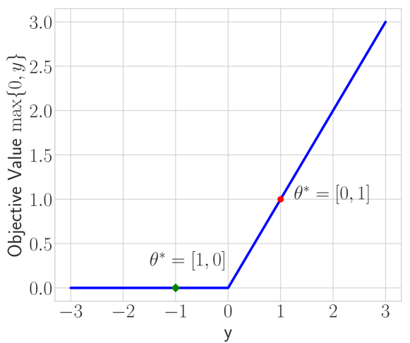
Figure 1: An example of objective in problem (B) with $f(y)=0$, $g(y)=0$ and $\bar{g}(y)=y$. The red point corresponds to $y=1$ and the green point corresponds to $y=-1$.

We will formulate the above optimization problem in equation (B) as a two player min-max game where one player seeks to minimize the following objective in $y\in Y$ and the other player maximizes the objective in $\theta=[\theta_{1},\theta_{2}]^{T}\in\Delta_{2}$ where $\Delta_{2}$ denotes the $2$-dimensional simplex:

$$\min_{y\in Y}f(y)+\max_{\theta\in\Delta_{2}}(\theta_{1}g_{1}(y)+\theta_{2}g_{2}(y))$$ (2)

Observe that the inner maximization objective in problem 2 is linear in $\theta\in\Delta_{2}$. Hence for any $y\in Y$ if both $g_{1}(y)$ and $g_{2}(y)$ are not zero, the optimal $\theta^{*}$ will lie on the boundary of the simplex [13], specifically one of $\theta_{1},\theta_{2}$ should be $1$ and the other $0$. In the case where both $g_{1}(y)=0$ and $g_{2}(y)=0$, problem (B) and problem 2 are trivially equivalent. Substituting $\theta^{*}$ in the objective in problem 2 it reduces to $f(y)+\max(g_{1}(y),g_{2}(y))$, the objective in problem (B). Thus, any solution of problem 2 is also a solution of the problem (B).

However, this equivalence is not useful since the term $\max_{\theta\in\Delta_{2}}(\theta_{1}g_{1}(y)+\theta_{2}g_{2}(y))$ could be highly non-smooth in $y$, which results in $\theta^{*}$ varying drastically with changing $y$. An example of such behavior is shown in Figure 1, where if $y$ is changed between any two values across $y=0$ then $\theta^{*}$ oscillates between $[0,1]$ and $[1,0]$. Borrowing insights from online convex optimization [14], we stabilize it by adding a regularization term that penalizes deviations from the previous estimate for $\theta$. More precisely, if we solve problem 2 iteratively and at any iteration $k$, we have an estimate $\theta^{k-1}$ then we seek to optimize the following objective for the $k$-th iteration

$$\min_{y\in Y}f(y)+\max_{\theta\in\Delta_{2}}(\theta_{1}g_{1}(y)+\theta_{2}g_{2}(y)-\eta^{k}\mathtt{KL}(\theta||\theta^{k}))$$ (3)

where $\eta^{k}\geq 0$ is the penalty coefficient at iteration $k$ and $\mathtt{KL}(\theta||\theta^{k})$ is the KL-divergence regularization term that penalizes deviation of $\theta$ from the previous estimate $\theta^{k}$ given by

$$\mathtt{KL}(\theta||\theta^{k})=\theta_{1}\log\frac{\theta_{1}}{\theta^{k}_{1}}+\theta_{2}\log\frac{\theta_{2}}{\theta^{k}_{2}}$$ (4)

for any $\theta,\theta^{k}\in\Delta_{2}$.

Note that the objective in problem 3 is an approximation of the objective in problem 2 (and hence, problem (B)) and is exact when $\eta^{k}=0$. To rectify this, we will solve the approximate objective iteratively for a decreasing sequence $\{\eta^{k}\}$ where $\eta^{k}\rightarrow 0$ as $k\rightarrow\infty$. Thus, in the limit the solution to the approximate objective is the same as the original objective.

It is important to note that the inner maximization w.r.t $\theta$ in problem 3 can be solved in closed form. Writing the Lagrangian and solving the KKT conditions [16], we get the following iterative update for $\theta$ at any iteration $k$,

$$\theta^{k}=\frac{\theta^{k-1}\exp({\frac{g(y)}{\eta^{k}}})}{\sum_{i=1}^{2}\theta^{k-1}_{i}\exp({\frac{g_{i}(y)}{\eta^{k}}})}$$ (5)

where we denote $g(y)=[g_{1}(y),g_{2}(y)]^{T}\in\mathbb{R}^{2}$, and $\theta^{k}=[\theta_{1}^{k},\theta_{2}^{k}]^{T}\in\Delta_{2}$. We can obtain $y^{k}$ by substituting update 5 into the objective in problem 3 resulting in the following optimization problem at any iteration $k$,

$$\min_{y\in Y}f(y)+\eta^{k}\log(\theta_{1}^{k-1}\exp({\frac{g_{1}(y)}{\eta^{k}}})+\theta_{2}^{k-1}\exp({\frac{g_{2}(y)}{\eta^{k}}}))$$ (6)

This results in an implicit update for $y$ that accounts for the $\theta$ update. This is reminiscent of implicit online learning [17], which typically has faster convergence and is robust in adversarial settings. The solution $y^{k}$ obtained from solving problem 6 can then be substituted into the update in problem 5 to get $\theta^{k}$. Let us denote the objective in equation 6 as $\mathcal{L}_{\eta^{k}}(y,\theta^{k-1})$. It is useful to observe that the objective $\mathcal{L}_{\eta^{k}}$ is smooth and twice-differentiable in $y$. Thus for each iteration $k$, we obtain a smoothed approximation of the objective in problem (B) and as $\eta^{k}\rightarrow 0$ we get a tighter approximation. We would like to emphasize that the proposed solver Tron exploits the structure of problem (B) by restricting $\theta$ to be in the simplex, and by using KL-divergence as the regularization. This trick has connections to exponentiated gradient descent [16], which also uses KL-divergence as regularization to perform efficient optimization on a simplex. As we will see in the experiments, this enables Tron to quickly solve problem (B). Tron is also related to proximal methods [18] and augmented lagrangian methods [12]. The proposed iterative solver is summarized in Algorithm 1.

Algorithm 1 Tron for general structured non-smooth objectives

1:  Input: Number of iterations $K$, sequence $\{\eta^{k}\}$ such that $0\leq\eta^{k+1}\leq\eta^{k}$ and $\eta^{k}\rightarrow 0$, sequence $\{\epsilon^{k}\}$ such that $\epsilon^{k}\geq 0$ and $\epsilon^{k}\rightarrow 0$

2:  Initialize $\theta^{0}\in\Delta_{2}$, $y^{0}\in Y$

3:  for $k=1$ to $K$ do

4:     Solve problem 6 (warm-starting from $y^{k-1}$) to obtain $y^{k}$ such that $\|\nabla_{y}\mathcal{L}_{\eta^{k}}(y^{k},\theta^{k-1})\|\leq\epsilon^{k}$

5:     Obtain $\theta^{k}$ using update 5 with $y=y^{k}$

6:  end for

7:  Return: Solution $y^{K}$

IV Convergence Analysis

In this section, we present convergence analysis for Tron described in Algorithm 1. We would like to show that as $k\rightarrow\infty$, every limit point of the sequence of solutions $\{y^{k}\}$ is a stationary point of the original problem (B). The following theorem states this guarantee:

Theorem 1 (Convergence under Inexact Minimization)

Assume $Y=\mathbb{R}^{n}$, and $f,g$ are continuously differentiable. For $k=1,\cdots$ let $y^{k}$ satisfy

$$\|\nabla_{y}\mathcal{L}_{\eta^{k}}(y^{k},\theta^{k-1})\|\leq\epsilon^{k}$$

where $\{\theta^{k}\}$ is bounded, and $\{\epsilon^{j}\}$ and $\{\eta^{k}\}$ satisfy

$$0\leq\eta^{k+1}\leq\eta^{k},\eta^{k}\rightarrow 0$$

$$0\leq\epsilon^{k},\epsilon^{k}\rightarrow 0$$

Then every limit point $y^{*}$ of the sequence $\{y^{k}\}$ is a stationary point of problem (B), i.e. $0\in\partial(f(y)+\max(g_{1}(y),g_{2}(y)))$ or $\nabla_{y}f(y^{*})+\lambda\nabla_{y}g_{1}(y^{*})+(1-\lambda)\nabla_{y}g_{2}(y^{*})=0$ for some $\lambda\in[0,1]$.

Proof:

Proof given in Appendix -A. ∎

Theorem 1 guarantees that Tron converges to a stationary point of problem (B). In Section V, we will show that this implies convergence to the global minimum of the trajectory optimization problem (A) when the dynamics are linear, and convergence to a stationary point when the dynamics are nonlinear.

V Application to Trajectory Optimization

In Section III we presented Tron, an iterative solver that can be used to efficiently solve problem (B). We will now show how Tron can be used to solve trajectory optimization problem (A) when the cost functions are non-smooth with smooth components. Let us rewrite problem (A) to accommodate the structure from equation 1 in the cost function as follows (using $M=1$ for ease of notation):

$$\min_{x_{0:T},u_{0:T}} \sum_{t=0}^{T}f_{t}(x_{t},u_{t})+\max\{g_{t}(x_{t},u_{t}),\bar{g}_{t}(x_{t},u_{t})\}$$ (7)

subject to $$x_{t+1}=\kappa(x_{t},u_{t})$$

where $f_{T}(x,u)=f_{T}(x)$, $g_{T}(x,u)=g_{T}(x)$, and $\bar{g}_{T}(x,u)=\bar{g}_{T}(x)$. Observe that the above objective is of the same form as the objective in problem (B). Hence, we can use Tron to optimize the above problem. Formulating the above problem as a min-max game as in Section III, we get the following objective in the state-control inputs at iteration $k$,

$$\min_{x_{0:T},u_{0:T}} \quad\sum_{t=0}^{T}f_{t}(x_{t},u_{t})+\eta^{k}\log(\theta_{t}^{k-1}\exp({\frac{g_{t}(x_{t},u_{t})}{\eta^{k}}})$$ (8)

$$~{}~{}~{}~{}~{}~{}~{}~{}~{}~{}~{}~{}~{}~{}~{}~{}~{}~{}~{}~{}~{}~{}~{}~{}~{}~{}~{}~{}~{}+\bar{\theta}^{k-1}_{t}\exp({\frac{\bar{g}_{t}(x_{t},u_{t})}{\eta^{k}}}))$$

subject to $$\quad x_{t+1}=\kappa(x_{t},u_{t})$$

Notice that unlike problem 6, we have a dynamics constraint $x_{t+1}=\kappa(x_{t},u_{t})$. We account for this by using Ilqr [10] to optimize the objective in problem 8, thereby implicitly enforcing the dynamics constraint in our solver. We use the control trajectory from the previous iteration to warm-start Ilqr at the current iteration to ensure it remains fast. The entire procedure to solve the trajectory optimization problem 7 using Tron is described in Algorithm 2.

Algorithm 2 Trajectory Optimization with Structured Non-smooth Cost Functions using Tron

1:  Input: Initial state $x_{0}$, initial control sequence $u^{0}_{0:T-1}$, sequence $\{\eta^{k}\}$, Number of iterations $K$

2:  Initialize $[\theta_{t}^{0},\bar{\theta}_{t}^{0}]^{T}\in\Delta_{2}$ for $t=0,\cdots,T$

3:  Compute $x_{0:T}^{0}\leftarrow$ Rollout dynamics $\kappa$ from $x_{0}$ using $u_{0:T-1}$

4:  for $k=1$ to $K$ do

5:     $x^{k}_{0:T},u^{k}_{0:T-1}\leftarrow$ Solution of Ilqr problem 8

6:     Obtain $[\theta_{t}^{k},\bar{\theta}_{t}^{k}]^{T}\in\Delta_{2}$ for $t=0,\cdots,T$ using update 5

7:  end for

8:  Return: $x_{0:T}^{K},u_{0:T-1}^{K-1}$

We can use Theorem 1 to analyze the convergence properties of Algorithm 2. Observe that when the dynamics $\kappa$ are linear, problem 7 is convex. Using the fact that any stationary point of a convex problem is a global minimum in conjunction with Theorem 1, we can guarantee that Tron converges to the global minimum of problem 7 when dynamics $\kappa$ are linear. However, when the dynamics $\kappa$ are arbitrarily nonlinear, then we lose convexity of problem 7 and Tron is only guaranteed to converge to a stationary point.

VI Experiments

In this section, we will evaluate the empirical performance of Tron against baselines on four tasks: lasso problem with synthetic data(VI-A), collision-free motion planning for a mobile robot(VI-B), sparse optimal control for a surgical steerable needle(VI-C), and a satellite rendezvous problem(VI-D). Tron and other baselines are implemented in Python on a $3.1$GHz Intel Core i5 machine, and the code is released at https://github.com/vvanirudh/TRON.

VI-A Lasso Problem with Synthetic Data

In this experiment, we will solve a $2$D lasso problem given as follows:

$$\min_{w}\frac{1}{N}\|Xw-y\|_{2}^{2}+\rho\|w\|_{1}$$ (9)

where $N=1000,X\in\mathbb{R}^{1000\times 2}$, $y\in\mathbb{R}^{1000}$ and $\rho\in\mathbb{R}^{+}$ are synthetically generated. We use $\rho=0.05$ for this experiment. We implemented Tron with Newton’s method to solve sub-problems 6, and compare it with Newton’s method on the non-smooth problem 9 and subgradient method. For the subgradient method, initial learning rate is chosen carefully and is decayed at $\mathcal{O}(\frac{1}{\sqrt{k}})$ where $k$ is the iteration number. We implement Newton’s method using a backtracking line search to compute the newton direction. For Tron, we use $\eta^{0}=1$ and update $\eta^{k+1}=0.9\eta^{k}$ for each iteration $k$.

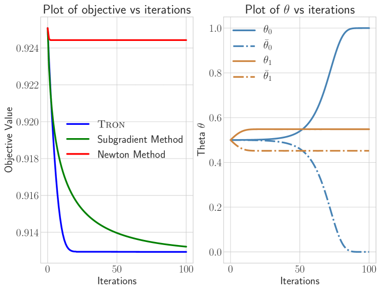
Figure 2: Performance of Tron, subgradient method and Newton’s method on the $2$D lasso problem. On the left, we plot the objective value vs iterations of each method. On the right, we plot how the dual variables $\theta$ vary across iterations.

The results are shown in Figure 2. As the objective in problem 9 is not differentiable, once we approach close to the minimum Newton’s method gets stuck as line search returns extremely small steps. This results in Newton’s method having extremely slow convergence as shown in Figure 2 (left). Subgradient method, on the other hand, does not rely on line search and with the help of decaying learning rate makes steady but slow progress towards the minimum. Tron, using Newton’s method to optimize the adaptively smoothed objective, quickly converges to the global minimum of the problem. In Figure 2 (right), we plot the dual variables $\theta$ as they vary across iterations. We start with initial values of $0.5$ for all the dual variables. The converged value of $w$ for Tron is $[-0.0005,0]$, and as expected the corresponding dual variables for each dimension converge to $1,0$ for the non-zero component and to values in $[0,1]$ for the zero component. See the proof of Theorem 1 in Appendix -A for theoretical insights on the final converged value of the dual variables.

VI-B Collision-Free Motion Planning for a Mobile Robot

Our second experiment involves a simulated differential drive mobile robot. The state is defined by vector ${x}=[p_{x},p_{y},\theta]^{T}\in\mathbb{R}^{3}$ where $(p_{x},p_{y})$ describes the robot’s two-dimensional position, $\theta$ is its orientation, and the control input is defined by the vector ${u}=[v_{l},v_{r}]^{T}\in\mathbb{R}^{2}$ where $v_{l},v_{r}$ describes the left and right wheel speeds (m/s) respectively. The dynamics of the robot are given by the following equations, $\dot{p_{x}}=\frac{1}{2}(v_{l}+v_{r})\cos\theta$, $\dot{p_{y}}=\frac{1}{2}(v_{l}+v_{r})\sin\theta$, and $\dot{\theta}=(v_{r}-v_{l})/w$, where $w$ is the distance between the wheels of the robot. This setup is very similar to the experimental setup used in [19]. We discretize the dynamics using a third-order Runge Kutta integrator.

The circular robot is moving in an environment with $O=11$ obstacles (see Figure 3 left) and needs to move from a specified start state to a goal state while avoiding collision with obstacles. We use the following cost functions in problem (A) to achieve this objective,

$$\ell_{0}({x}_{0},{u}_{0})=({x}_{0}-{s})^{T}Q({x}_{0}-{s})+({u}_{0}-{\bar{u}})^{T}R({u}_{0}-{\bar{u}})$$

$$\ell_{t}({x}_{t},{u}_{t})=({u}_{t}-{\bar{u}})^{T}R({u}_{t}-{\bar{u}})+\rho\sum_{i=1}^{O}\max\{0,-\nu d_{i}({x}_{t})\}$$

$$\ell_{T}({x}_{t})=({x}_{t}-{g})^{T}Q({x}_{t}-{g})$$

where ${g}$ is the goal state, ${s}$ is the start state, $T$ is the horizon, and ${\bar{u}}$ is the nominal control input. $\rho,\nu$ are positive scalar factors, and the function $d_{i}({x})$ gives the signed distance between the robot at state ${x}$ and the $i$-th obstacle of the environment. Note that we penalize a trajectory if it results in the robot penetrating an obstacle (thus, $d_{i}({x})$ is negative for any $i$), and zero cost if the robot does not collide with any of the obstacles. Note that this cost function is non-smooth and convex.

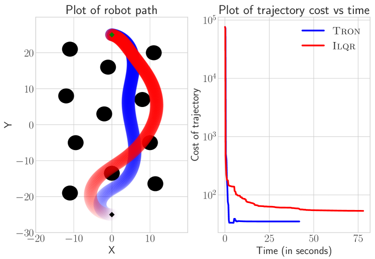
Figure 3: Performance of Tron and Ilqr for trajectory optimization of a differential drive robot. On the left, the resulting trajectory from both Tron (blue) and Ilqr (red) are shown (lighter the color, earlier the time step). The start position is depicted using black diamond, and the goal position is depicted using green diamond. On the right, we plot the cost vs time (in seconds) for both methods. Both methods are run for $200$ iterations.

We compare Tron (with a fixed $\eta^{k}=1$ for all iterations) with a baseline that uses Ilqr on the non-smooth objective. The results are shown in Figure 3. Ilqr exhibits extremely slow convergence and does not converge to a collision-free path as shown in Figure 3 (left). On the other hand, Tron quickly converges to a collision-free path with a significantly lower cost compared to Ilqr. Note that the y-axis in Figure 3 (right) is in log-scale. It is also interesting to observe the path Tron converges to. Since the cost function $\ell_{t}$ only penalizes if the robot collides with the obstacle and zero penalty otherwise, we see that the resulting path narrowly avoids collision with obstacles, and leads the robot directly to the goal between the obstacles on a low-cost trajectory.

VI-C Sparse Optimal Control for a Surgical Steerable Needle

Our third experiment involves a simulated bevel-tip surgical steerable needle that is highly underactuated and non-holonomic [20]. Planning the motion of the needle is a challenging problem as it can only be controlled from its base through insertion and twisting. We use the motion model proposed in [21] where the state of the needle $x=[p_{x},p_{y},p_{z},\alpha,\beta,\gamma]^{T}\in\mathbb{R}^{6}$ is represented by a transformation matrix $X\in SE(3)$:

$$X=\begin{bmatrix}R&p\\ 0&1\end{bmatrix}$$

where $R\in SO(3)$ is a $3\times 3$ rotation matrix describing needle’s orientation constructed from $[\alpha,\beta,\gamma]^{T}$ which is the euler angle representation, and $p=[p_{x},p_{y},p_{z}]^{T}\in\mathbb{R}^{3}$ describes its position. The control input $u=[v,w,\delta]^{T}\in\mathbb{R}^{3}$ is represented as:

$$U=\begin{bmatrix}W&V\\ 0&1\end{bmatrix},~{}~{}~{}~{}~{}W=\begin{bmatrix}0&-w&0\\ w&0&-v\delta\\ 0&v\delta&0\end{bmatrix}$$

where $V=[0,0,v]^{T}$, $v$ is the linear velocity of the needle tip (m/s), $w$ is the angular speed of the needle base (rad/s), and $\delta$ is the desired curvature of the needle. The kinematics of the needle are given by $\dot{X}=XU$. This setup is very similar to the experimental setup used in [22].

The task is to plan a path for the needle from a fixed start state to a goal state ensuring kinematic feasibility. In addition, we would also like sparsity in the angular speed $w$ control as rotation of the needle inside a body increases trauma to patient tissues. We use very similar objectives as in Section VI-B except the following:

$$\ell_{t}(x_{t},u_{t})=(u_{t}-\bar{u})^{T}R(u_{t}-\bar{u})+\rho|w|$$

where $u=[v,w,\delta]^{T}$ and $\rho$ is a positive scalar. Thus, we penalize the absolute value (or L1-norm) of the angular speed $w$ to enforce sparsity in the resulting trajectory for that control input. This cost function is convex but non-smooth.

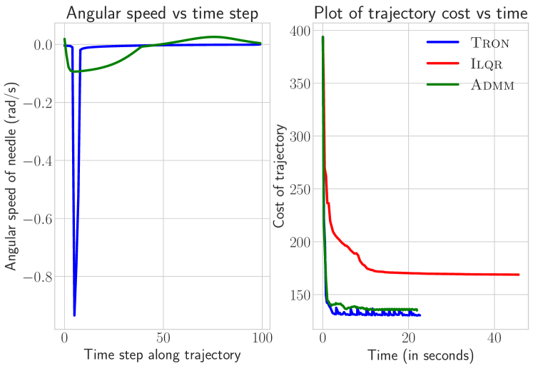
Figure 4: Performance of Tron, Admm, and Ilqr on the surgical needle task. On the right, we plot the cost of the trajectory vs time (in seconds) for all the methods. On the left, we show the angular speed control sequence for the final converged trajectory for Tron and Admm methods. We do not show Ilqr as it does not exhibit any sparse behavior. All approaches are run for $100$ iterations.

We compare Tron (with a fixed $\eta^{k}=0.3$ for all iterations) with a baseline that uses Ilqr on the non-smooth objective. In addition, we also implement the Admm approach proposed by Le Cleac’h and Manchester [8] which accounts for the L1-norm penalty. The results are shown in Figure 4. As expected on non-smooth objectives, Ilqr exhibits slow convergence and we have noticed that it does not result in a trajectory that has sparse angular speed control. Admm, on the other hand, accounts for the L1-norm penalty and shows fast convergence behavior. As shown in Figure 4 (right), it converges to a trajectory that has significantly lower cost compared to Ilqr. Tron also exhibits fast convergence behavior similar to Admm and as shown in Figure 4 (left), it does a much better job at enforcing sparsity in angular speed of the needle in the final trajectory, (in fact, Admm does not achieve any sparsity in its final trajectory) and achieves lower final trajectory cost.

VI-D Satellite Rendezvous Problem

Our last experiment involves a simulated satellite rendezvous problem. These satellites rely on reaction control system thrusters for control which can only operate inside a limited range, and are suitable for a bang-off-bang control strategy. Thus, enforcing sparsity in control is desirable to achieve this strategy. The objective of this task is to control a chaser satellite so that it approaches and docks onto a target satellite. We borrow the linearized version of this problem from [8] in which the state vector $x=[p_{1},p_{2},p_{3},\dot{p}_{1},\dot{p}_{2},\dot{p}_{3}]\in\mathbb{R}^{6}$, where $[p_{1},p_{2},p_{3}]^{T}$ is the position and $[\dot{p}_{1},\dot{p}_{2},\dot{p}_{3}]^{T}$ is the velocity, both expressed in a frame centered on the target satellite. The control input $u$ is the force applied on the satellite, and the model is given as follows:

$$\dot{x}=\begin{bmatrix}\dot{p}_{1}\\ \dot{p}_{2}\\ \dot{p}_{3}\\ 3n^{2}p_{1}+2np_{2}+u_{1}/m\\ -2n\dot{p}_{1}+u_{2}/m\\ -n^{2}p_{3}+u_{3}/m\end{bmatrix}$$

where $n$ is the mean motion of the target satellite’s orbit and $m$ is the satellite’s mass. This setup is similar to the setup used in [8] with small modifications.

The objective of the task is for the chaser satellite to reach the state $[0,0,0,0,0,0]^{T}$ (which is the target satellite’s position and zero velocity) by the end of the trajectory horizon. We use the following cost functions in problem (A) to achieve this objective,

$$\ell_{t}(x_{t},u_{t}) =\alpha\|u_{t}\|_{1}+u_{t}^{T}Ru_{t}$$

$$\ell_{T}(x_{T}) =x_{T}^{T}Qx_{T}$$

for $0\leq t\leq T-1$. Thus, the objective function enforces that the chaser satellite reaches the target and uses sparse controls to achieve it.

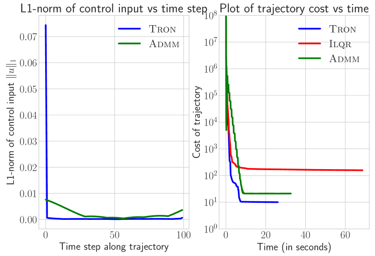
Figure 5: Performance of Tron, Admm, and Ilqr on the satellite rendezvous problem. On the right, we plot the cost of trajectory vs time (in seconds) for all the methods. On the left, we show L1-norm of the control input sequence in the final trajectory for Admm and Tron. We do not show Ilqr as it does not exhibit any sparse behavior. All approaches are run for $300$ iterations.

We compare Tron (with a fixed $\eta^{k}=0.1$ for all iterations) with Ilqr and Admm. The results are shown in Figure 5. Interestingly, Ilqr exhibits fast convergence initially until it reaches close to the minimum where the non-smoothness of the objective results in extremely small updates and slow convergence (See Figure 5 right). Admm also has extremely fast convergence at the start and then increases the cost for a few iterations before converging to a lower cost compared to ilqr. However, Tron exhibits the fastest convergence among all and quickly reaches a significantly lower cost. In Figure 5 (left), we plot the L1-norm of the control sequence for the final trajectory in the case of Admm and Tron. We refrain from plotting the L1-norm for Ilqr as its final trajectory does not exhibit any sparse behavior and thus, is very undesirable for RCS control. As shown in the plot, Tron converges to a final trajectory that uses the thrusters at the beginning and then simply coasts for the rest of the trajectory without using the thrusters. This behavior is ideal for RCS thrusters. Admm, on the other hand, converges to a trajectory that exhibits significantly less sparsity and thus, has higher cost.

VII Extensions and Conclusion

The proposed solver Tron can be extended in several ways. Firstly, we can account for arbitrary non-linear constraints $\alpha,\beta$ in problem (A) by using augmented lagrangian techniques such as the ones used in Plancher et. al. [23]. Secondly, Tron is easily extensible to cost functions where there are more than two functions involved in the $\max$ operator. In such a case, the dual variables would lie in a higher dimensional simplex but we still achieve fast convergence since we are exploiting the structure. Finally, Tron can be made numerically more robust by employing techniques proposed in Howell et. al. [24] such as using square-root backward pass in Ilqr.

In conclusion, this work has proposed a fast solver Tron that can be used as a general purpose tool in trajectory optimization where the cost functions are non-differentiable with differentiable components. Tron exhibits fast convergence behavior because it exploits the structure of the cost function to construct a sequence of adaptively smoothed objectives that can each be optimized efficiently. Tron is provably guaranteed to converge to the global optimum in the case of convex costs and linear dynamics, and to a stationary point in the case of non-linear dynamics. Empirically, we show that Tron outperforms other trajectory optimization approaches in simulated planning and control tasks.

-A Proof of Theorem 1

Consider the quantity $\nabla_{y}\mathcal{L}_{\eta^{k}}(y^{k},\theta^{k-1})$ for any iteration $k\geq 1$. Using equation 6 we have,

$$\nabla_{y}\mathcal{L}_{\eta^{k}}(y^{k},\theta^{k-1})=\nabla_{y}f(y^{k})+$$

$$\frac{\theta_{1}^{k-1}\exp(\frac{g_{1}(y^{k})}{\eta^{k}})\nabla_{y}g_{1}(y^{k})+\theta_{2}^{k-1}\exp(\frac{g_{2}(y^{k})}{\eta^{k}})\nabla_{y}g_{2}(y^{k})}{\theta_{1}^{k-1}\exp(\frac{g_{1}(y^{k})}{\eta^{k}})+\theta_{2}^{k-1}\exp(\frac{g_{2}(y^{k})}{\eta^{k}})}$$

$$=\nabla_{y}f(y^{k})+$$

$$\frac{\theta_{1}^{k-1}\exp(\frac{g_{1}(y^{k})}{\eta^{k}})}{\theta_{1}^{k-1}\exp(\frac{g_{1}(y^{k})}{\eta^{k}})+\theta_{2}^{k-1}\exp(\frac{g_{2}(y^{k})}{\eta^{k}})}\nabla_{y}g_{1}(y^{k})+$$

$$\frac{\theta_{2}^{k-1}\exp(\frac{g_{2}(y^{k})}{\eta^{k}})}{\theta_{1}^{k-1}\exp(\frac{g_{1}(y^{k})}{\eta^{k}})+\theta_{2}^{k-1}\exp(\frac{g_{2}(y^{k})}{\eta^{k}})}\nabla_{y}g_{2}(y^{k})$$

Let us denote $\lambda_{k}=\frac{\theta_{1}^{k-1}\exp(\frac{g_{1}(y^{k})}{\eta^{k}})}{\theta_{1}^{k-1}\exp(\frac{g_{1}(y^{k})}{\eta^{k}})+\theta_{2}^{k-1}\exp(\frac{g_{2}(y^{k})}{\eta^{k}})}$, then it is easy to see that $1-\lambda_{k}=\frac{\theta_{2}^{k-1}\exp(\frac{g_{2}(y^{k})}{\eta^{k}})}{\theta_{1}^{k-1}\exp(\frac{g_{1}(y^{k})}{\eta^{k}})+\theta_{2}^{k-1}\exp(\frac{g_{2}(y^{k})}{\eta^{k}})}$. Then we can rewrite, the above equation as,

$$\nabla_{y}\mathcal{L}_{\eta^{k}}(y^{k},\theta^{k-1})=\nabla_{y}f(y^{k}) +\lambda_{k}\nabla_{y}g_{1}(y^{k})+$$

$$(1-\lambda_{k})\nabla_{y}g_{2}(y^{k})$$ (10)

Take the limit of the above equation as $k\rightarrow\infty$,

$$\lim_{k\rightarrow\infty}\nabla_{y}\mathcal{L}_{\eta^{k}}(y^{k},\theta^{k-1})=\nabla_{y}f(y^{*}) +\lim_{k\rightarrow\infty}\lambda_{k}\nabla_{y}g_{1}(y^{*})+$$

$$(1-\lim_{k\rightarrow\infty}\lambda_{k})\nabla_{y}g_{2}(y^{*})$$ (11)

The hypothesis implies that $\lim_{k\rightarrow\infty}\nabla_{y}\mathcal{L}_{\eta^{k}}(y^{k},\theta^{k-1})\rightarrow 0$. Thus all that remains to show is that $\lim_{k\rightarrow\infty}\lambda_{k}$ is finite. This is easy to prove. Note that for the limit point $y^{*}$ there are one of three possibilities: $g_{1}(y^{*})>g_{2}(y^{*})$, $g_{1}(y^{*})<g_{2}(y^{*})$, or $g_{1}(y^{*})=g_{2}(y^{*})$. We will show the argument for one of these possibilities and the other two are very similar. Assume $g_{1}(y^{*})>g_{2}(y^{*})$ then we have that

$$\lim_{k\rightarrow\infty}\lambda_{k} =\lim_{k\rightarrow\infty}\frac{\theta_{1}^{k-1}\exp(\frac{g_{1}(y^{k})}{\eta^{k}})}{\theta_{1}^{k-1}\exp(\frac{g_{1}(y^{k})}{\eta^{k}})+\theta_{2}^{k-1}\exp(\frac{g_{2}(y^{k})}{\eta^{k}})}$$

$$=\lim_{k\rightarrow\infty}\frac{1}{1+\frac{\theta^{k-1}_{2}}{\theta_{1}^{k-1}}\exp(\frac{g_{2}(y^{k})-g_{1}(y^{k})}{\eta^{k}})}$$

$$=\frac{1}{1+\lim_{k\rightarrow\infty}\frac{\theta_{2}^{k-1}}{\theta_{1}^{k-1}}\exp(\frac{g_{2}(y^{*})-g_{1}(y^{*})}{\lim_{k\rightarrow\infty}\eta^{k}})}$$

$$=1$$

The last equality is obtained using the fact that $g_{1}(y^{*})>g_{2}(y^{*})$ and $\eta^{k}\rightarrow 0$. Similarly, we can prove that $\lim_{k\rightarrow\infty}\lambda_{k}=0$ when $g_{1}(y^{*})<g_{2}(y^{*})$, and $\lim_{k\rightarrow\infty}\lambda_{k}=\lim_{k\rightarrow\infty}\frac{\theta_{1}^{k-1}}{\theta^{k-1}_{1}+\theta_{2}^{k-1}}=\theta_{1}^{k-1}$ when $g_{1}(y^{*})=g_{2}(y^{*})$. Note that the sequence $\{\theta^{k}\}$ is bounded as they all lie in a simplex $\Delta_{2}$, thus $\lim_{k\rightarrow\infty}\theta_{1}^{k-1}$ is finite and lies in $[0,1]$. Hence, we have that there exists some $\lambda\in[0,1]$ such that for every limit point $y^{*}$ of the sequence $\{y^{k}\}$ satisfying the assumptions in the theorem,

$$\nabla_{y}f(y^{*})+\lambda\nabla_{y}g_{1}(y^{*})+(1-\lambda)\nabla_{y}g_{2}(y^{*})=0$$ (12)

$\blacksquare$

References

- [1] J. T. Betts, “Survey of numerical methods for trajectory optimization,” Journal of Guidance, Control, and Dynamics, vol. 21, no. 2, pp. 193–207, 1998. [Online]. Available: https://doi.org/10.2514/2.4231
- [2] M. Zucker, N. D. Ratliff, A. D. Dragan, M. Pivtoraiko, M. Klingensmith, C. M. Dellin, J. A. Bagnell, and S. S. Srinivasa, “CHOMP: covariant hamiltonian optimization for motion planning,” I. J. Robotics Res., vol. 32, no. 9-10, pp. 1164–1193, 2013. [Online]. Available: https://doi.org/10.1177/0278364913488805
- [3] R. Tibshirani, “Regression shrinkage and selection via the lasso,” Journal of the Royal Statistical Society: Series B (Methodological), vol. 58, no. 1, pp. 267–288, 1996. [Online]. Available: https://rss.onlinelibrary.wiley.com/doi/abs/10.1111/j.2517-6161.1996.tb02080.x
- [4] I. Ross, How to Find Minimum-Fuel Controllers. [Online]. Available: https://arc.aiaa.org/doi/abs/10.2514/6.2004-5346
- [5] L. Bako, D. Chen, and S. Lecoeuche, “A numerical solution to the minimum-time control problem for linear discrete-time systems,” CoRR, vol. abs/1109.3772, 2011. [Online]. Available: http://arxiv.org/abs/1109.3772
- [6] G. Vossen and H. Maurer, “On l1-minimization in optimal control and applications to robotics,” Optimal Control Applications and Methods, vol. 27, no. 6, pp. 301–321, 2006. [Online]. Available: https://onlinelibrary.wiley.com/doi/abs/10.1002/oca.781
- [7] J. van den Berg, “Iterated LQR smoothing for locally-optimal feedback control of systems with non-linear dynamics and non-quadratic cost,” in American Control Conference, ACC, 2014, pp. 1912–1918. [Online]. Available: https://doi.org/10.1109/ACC.2014.6859404
- [8] S. Le Cleac’h and Z. Manchester, “Fast solution of optimal control problems with l1 cost,” 2019. [Online]. Available: https://rexlab.stanford.edu/papers/l1-cost-optimizer.pdf
- [9] S. P. Boyd, N. Parikh, E. Chu, B. Peleato, and J. Eckstein, “Distributed optimization and statistical learning via the alternating direction method of multipliers,” Foundations and Trends in Machine Learning, vol. 3, no. 1, pp. 1–122, 2011. [Online]. Available: https://doi.org/10.1561/2200000016
- [10] W. Li and E. Todorov, “Iterative linear quadratic regulator design for nonlinear biological movement systems,” in Proceedings of the First International Conference on Informatics in Control, Automation and Robotics, 2004, pp. 222–229. [Online]. Available: https://homes.cs.washington.edu/~todorov/papers/LiICINCO04.pdf
- [11] D. Mayne, “A second-order gradient method for determining optimal trajectories of non-linear discrete-time systems,” International Journal of Control, vol. 3, no. 1, pp. 85–95, 1966. [Online]. Available: https://doi.org/10.1080/00207176608921369
- [12] M. R. Hestenes, “Multiplier and gradient methods,” Journal of optimization theory and applications, vol. 4, no. 5, pp. 303–320, 1969. [Online]. Available: https://doi.org/10.1007/BF00927673
- [13] D. Bertsimas and J. Tsitsiklis, Introduction to Linear Optimization, 1st ed. Athena Scientific, 1997. [Online]. Available: https://dl.acm.org/doi/book/10.5555/548834
- [14] E. Hazan, “Introduction to online convex optimization,” CoRR, vol. abs/1909.05207, 2019. [Online]. Available: http://arxiv.org/abs/1909.05207
- [15] W. Karush, “Minima of functions of several variables with inequalities as side conditions,” Master’s thesis, Department of Mathematics, University of Chicago, Chicago, IL, USA, 1939.
- [16] J. Kivinen and M. K. Warmuth, “Exponentiated gradient versus gradient descent for linear predictors,” Inf. Comput., vol. 132, no. 1, pp. 1–63, 1997. [Online]. Available: https://doi.org/10.1006/inco.1996.2612
- [17] B. Kulis and P. L. Bartlett, “Implicit online learning,” in Proceedings of the 27th International Conference on Machine Learning (ICML-10), June 21-24, 2010, Haifa, Israel, 2010, pp. 575–582. [Online]. Available: https://icml.cc/Conferences/2010/papers/429.pdf
- [18] N. Parikh and S. P. Boyd, “Proximal algorithms,” Foundations and Trends in Optimization, vol. 1, no. 3, pp. 127–239, 2014. [Online]. Available: https://doi.org/10.1561/2400000003
- [19] J. van den Berg, “Extended LQR: locally-optimal feedback control for systems with non-linear dynamics and non-quadratic cost,” in The 16th International Symposium on Robotics Research ISRR, 2013, pp. 39–56. [Online]. Available: https://doi.org/10.1007/978-3-319-28872-7_3
- [20] V. Duindam, R. Alterovitz, S. Sastry, and K. Y. Goldberg, “Screw-based motion planning for bevel-tip flexible needles in 3d environments with obstacles,” in International Conference on Robotics and Automation, ICRA, 2008, pp. 2483–2488. [Online]. Available: https://doi.org/10.1109/ROBOT.2008.4543586
- [21] R. J. W. III, J. S. Kim, N. J. Cowan, G. S. Chirikjian, and A. M. Okamura, “Nonholonomic modeling of needle steering,” I. J. Robotics Res., vol. 25, no. 5-6, pp. 509–525, 2006. [Online]. Available: https://doi.org/10.1177/0278364906065388
- [22] J. van den Berg, S. Patil, R. Alterovitz, P. Abbeel, and K. Y. Goldberg, “Lqg-based planning, sensing, and control of steerable needles,” in Algorithmic Foundations of Robotics IX - Selected Contributions of the Ninth International Workshop on the Algorithmic Foundations of Robotics, WAFR, 2010, pp. 373–389. [Online]. Available: https://doi.org/10.1007/978-3-642-17452-0_22
- [23] B. Plancher, Z. Manchester, and S. Kuindersma, “Constrained unscented dynamic programming,” in International Conference on Intelligent Robots and Systems, IROS, 2017, pp. 5674–5680. [Online]. Available: https://doi.org/10.1109/IROS.2017.8206457
- [24] T. A. Howell, B. E. Jackson, and Z. Manchester, “ALTRO: A fast solver for constrained trajectory optimization,” in International Conference on Intelligent Robots and Systems, IROS, 2019, pp. 7674–7679. [Online]. Available: https://doi.org/10.1109/IROS40897.2019.8967788