Iron Line from Neutron Star Accretion Disks in Scalar Tensor Theories

Abstract

The Fe ${\rm K}_{\alpha}$ fluorescent line at $6.4$ keV is a powerful probe of the space-time metric in the vicinity of accreting compact objects. We investigated here how some alternative theories of gravity, namely Scalar tensor Theories, that invoke the presence of a non-minimally coupled scalar field and predict the existence of strongly scalarized neutron stars, change the expected line shape with respect to General Relativity. By taking into account both deviations from the general relativistic orbital dynamics of the accreting disk, where the Fe line originates, and the changes in the light propagation around the neutron star, we computed line shapes for various inclinations of the disk with respect to the observer. We found that both the intensity of the low energy tails and the position of the high energy edge of the line change. Moreover we verified that even if those changes are in general of the order of a few percent, they are potentially observable with the next generation of X-ray satellites.

1 Introduction

Since the pioneering work of Brans & Dicke (1961), Scalar Tensor Theories (STTs) have always attracted large attention from the scientific community as viable gravitational extensions of General Relativity (GR) (Matsuda & Nariai, 1973; Damour & Esposito-Farese, 1993; Fujii & Maeda, 2003; Capozziello & de Laurentis, 2011), in part due to their mathematical simplicity, in part because they seem to avoid many of the pathologies of other extensions (Papantonopoulos, 2015). They key idea of STTs is to replace the gravitational coupling constant $G$, with a dynamical non-minimally coupled scalar field $\Phi$, such that the standard Einstein-Hilbert Lagrangian is modified to:

$$\mathcal{S}_{\rm stt}=\frac{1}{16\pi}\int\sqrt{-\tilde{g}}[\Phi\tilde{R}-\frac{\omega(\Phi)}{\Phi}\tilde{\nabla}_{\mu}\Phi\tilde{\nabla}^{\mu}\Phi-2\tilde{\Lambda}(\Phi)]d^{4}x,$$ (1)

where $\tilde{g}$ is the determinant of the metric tensor $\tilde{g}_{\mu\nu}$, $\tilde{\nabla}_{\mu}$ the related covariant derivative, $\tilde{R}$ the Ricci scalar, $\omega(\Phi)$ describes the field coupling and $\tilde{\Lambda}(\Phi)$ is the scalar field potential. The action of the scalar field $\Phi$ leads to non-linear behaviours that in principle could account for cosmological observations, without the need to invoke dark components (Capozziello & de Laurentis, 2011).

On top of the cosmological phenomenology associated to STTs, these theories make interesting predictions also in the regime of strong gravity, potentially leading to interesting deviations in the structure and properties (e.g. the mass-radius relation) of neutron stars (NSs) (Damour & Esposito-Farese, 1993). While solar-system experiments can set constraints on the scalar field in the weak gravitational regime (Shao et al., 2017), only compact objects can set limits in the strong one. Unfortunately, given that the no-hair theorem forbids black holes (BHs) to have any scalar charge (Hawking, 1972), the most promising environment to test gravity in the strong regime, binary BH mergers, cannot be used to set any constrain on the presence and nature of scalar fields (Berti et al., 2015). Only NSs offer an environment compact enough for the scalar field to emerge. Indeed, some of these theories predict that NSs can have sizeable scalar charges (Damour & Esposito-Farese, 1993), because of a phenomenon known as spontaneous scalarization. The presence of a scalar field leads to new wave modes in binary NSs systems, beyond the standard quadrupole gravitational wave emission. However, the present limits on STTs based on the study of the orbital decay of binary pulsars (Shao et al., 2017; Anderson, Freire & Yunes, 2019) can be easily accommodated introducing screening potentials or assuming massive scalar fields (Yazadjiev, Doneva & Popchev, 2016). On the other hand it is not clear how, and how much a scalar field modifies the final phases of binary NS inspiral before merger to a degree observable with current instruments, and with specific signatures that cannot be attributed to other causes (e.g. the equation of state). Even the measure of the mass radius relation might not prove to be enough, if limited to few objects, given its degeneracy with the equation of state. What we lack at present is a way to probe deviations from GR in the close vicinity of NSs.
One of the most powerful probes of the space time geometry close to compact objects is light propagation. Light bending has been widely used in binary pulsar systems (Demorest et al., 2010; Antoniadis et al., 2013), and more recently in the case of the BH at the center of M87 (Event Horizon Telescope Collaboration et al., 2019). In accreting systems, one can also use emission from the accretion disk, and in particular the shape of the Fe ${\rm K}_{\alpha}$ fluorescent line at $6.4$ keV (Miller, 2007; Dauser, García & Wilms, 2016). This line has been extensively used in acceting BHs to measure their spin (Risaliti et al., 2013; Parker, Miller & Fabian, 2018; Kammoun, Nardini & Risaliti, 2018). Recently its has also been investigated in alternative gravitational theories that predict deviation also for the BH metric (Yang, Ayzenberg & Bambi, 2018; Nampalliwar et al., 2018). Despite the fact that this technique has been used just for BHs, we know of many accreting NSs systems where we observe the presence of this line (Laor, 1991; Matt et al., 1992; Degenaar et al., 2015; Coughenour et al., 2018; Homan et al., 2018). In principle Fe ${\rm K}_{\alpha}$ could be used to constrain the metric properties outside the NS itself. Ghasemi-Nodehi (2018) has shown how to parametrize deviations from analytical solutions in GR, particularly relevant for rapidly rotating NSs where the metric is only known numerically. It has been suggested that the Fe line in accreting NSs could be used to set limit on the NS radius, by modeling the effect on the shape of the line due to the disk occultation by the surface of the NS itself (Cackett et al., 2008; La Placa et al., 2020). However in general these effects are found to be small, of the order of few percents, and thus not measurable with current instruments. They might in principle be within reach of next generation X-ray satellites (Barret et al., 2016). In the line of Sotani (2017), who investigates light propagation from hot spots on the surface of a scalarized NS, here we investigate how the Fe line emission from an accreting disk around a NS is modified by the presence of a scalar field with respect to GR, including the effect of the possible occultation/truncation of the disk by the NS itself. In order to simplify the discussion, this paper is mostly structured as a proof-of principle, and not as a full fledged investigation of the possible parameter space. For these reasons, neither we compute realistic NS models based on physical equation of states, nor we include rotation, and for the same reason we opted for the simplest STT, trying to parametrise the vacuum solution outside, in order to provide a flexible estimate of the expected changes.

This paper is organised as follows. In Sect.2 we briefly review STTs, present the metric expected outside a scalarized NSs, and introduce the ray-tracing. In Sect.3 we present and discuss the results both for unocculted and occulted systems. We conclude in Sect.4.

2 Metric and ray-Tracing in Vacuum STT

Depending on the nature and form of the coupling function $\omega(\Phi)$ or of the scalar field potential $\tilde{\Lambda}(\Phi)$ one can get different STTs, with different phenomenologies. The simplest case is that of a mass-less scalar field $\tilde{\Lambda}(\Phi)=0$. Varying the action with respect to the metric and scalar field leads to a coupled system of equations describing their mutual interplay. It can be easily shown that such system, and in particular the generalisation of Einstein field equations for the metric terms, contains higher order derivatives, that change the mathematical nature of the equations themselves (Santiago & Silbergleit, 2000).
It is possible however to recast the problem in terms of a minimally-coupled scalar field $\mathcal{X}$, by performing a conformal transformation from the original metric $\tilde{g}_{\mu\nu}$ to a new metric $\bar{g}_{\mu\nu}=\Phi\tilde{g}_{\mu\nu}$. Expressed in terms of this new field and new metric the Lagrangian reads:

$$\mathcal{S}_{\rm stt}=\frac{1}{16\pi}\int\sqrt{-\bar{g}}[\bar{R}-2\bar{\nabla}_{\mu}\mathcal{X}\bar{\nabla}^{\mu}\mathcal{X}-2\bar{\Lambda}(\mathcal{X})]d^{4}x,$$ (2)

where the bar indicates quantities relative to the new metric. This form leads to a set of field equations that are analogous to the standard Einstein equations, supplemented with a well behaved momentum-energy tensor for the scalar field. The original frame where the action read as in Eq. 1 is known as the Jordan frame while the one where it reads as in Eq. 2 is known as the Einstein frame. The relation between $\mathcal{X}$ and $\Phi$ is:

$$\sqrt{2}\frac{{\rm d}\mathcal{X}}{{\rm d}\ln{\Phi}}=\sqrt{\omega(\Phi)+3/2}.$$ (3)

In the simplest case of a mass-less scalar field, the field equations in vacuum become:

$$\bar{G}_{\mu\nu}=2\bar{\nabla}_{\mu}\mathcal{X}\bar{\nabla}_{\nu}\mathcal{X}-\bar{g}_{\mu\nu}\bar{\nabla}_{\kappa}\mathcal{X}\bar{\nabla}^{\kappa}\mathcal{X},$$ (4)

and

$$\bar{\nabla}_{\mu}\bar{\nabla}^{\mu}\mathcal{X}=0.$$ (5)

If one assumes steady state, $\partial_{t}=0$, and spherical symmetry (a reasonable approximation for NSs not rotating close to the break-up frequency), then it is possible to show that the line element in the Einstein frame can be written in spherical coordinates $[r,\theta,\phi]$ as (Just, 1959; Doneva et al., 2014):

$$ds^{2}=-f(r)^{a}dt^{2}+f(r)^{-a}dr^{2}+r^{2}f(r)^{1-a}[d\theta^{2}+\sin^{2}{\theta}d\phi^{2}]$$ (6)

where the function $f(r)$ and the exponent $a$ depend on the total mass $M$ and scalar charge $Q$ of the NS according to:

$$f(r)=\left(1-2\sqrt{M^{2}+Q^{2}}/r\right),\quad a=M/\sqrt{M^{2}+Q^{2}},$$ (7)

while the scalar field is:

$$\mathcal{X}=\frac{Q}{2\sqrt{M^{2}+Q^{2}}}\ln\left(1-2\sqrt{M^{2}+Q^{2}}/r\right).$$ (8)

However, in the Einstein frame, contrary to the Jordan frame, the weak equivalence principle does not hold. In order to compute ray-tracing using the standard geodesic equations, one needs to move back to the Jordan frame and, to do so, to know the relation between $\mathcal{X}$ and $\Phi$. One of the simplest possible choices is to take $\Phi={\rm Exp}[-2\alpha_{o}\mathcal{X}-\beta_{o}\mathcal{X}^{2}]$. $\alpha_{o}$ sets how strong deviations from GR are in the weak field regime, and Solar system experiments constrain it to be less than $\approx 10^{-4}$. $\beta_{o}$, on the other hand, sets how strong scalarization effects can be in compact objects, and if smaller than$\simeq-4$, it gives rise to strongly scalarized systems (Will, 2014). The Jordan metric is then fully parametrised by the quantities $M$, $Q$, $\alpha_{o}$, and $\beta_{o}$.

If one makes the further assumption $\alpha_{o}=0$, it is then possible to derive an analytical expression for the Keplerian frequency of matter orbiting the NS, using the effective potential approach (Abramowicz & Kluźniak, 2005; Doneva et al., 2014):

$$\Omega_{\rm k}=\frac{-\left(1-\frac{2M}{ar}\right)^{2a}[\frac{2M^{2}}{a}+\beta_{o}Q^{2}\ln\left(1-\frac{2M}{ar}\right)]}{r^{2}\left(1-\frac{2M}{ar}\right)[\frac{2M^{2}}{a}+\frac{2M^{2}}{a^{2}}-\frac{2Mr}{a}-\beta_{o}Q^{2}\ln\left(1-\frac{2M}{ar}\right)]},$$ (9)

which allows one to compute the radius of the innermost stable circular orbit (ISCO).
Once the metric and the four-velocity of matter orbiting in the disk are known it is possible to reconstruct the shape of the Fe line, as in Psaltis & Johannsen (2012). Given an observer that sees the NS-disk system at an inclination $\psi$ (the angle between the observer direction and the perpendicular to the disk plane) light rays are traced from an image plane at the location of the observer, until they reach the disk (or until the intercept the surface of the NS in those cases, and for those inclinations, for which the NS can occult/truncate the disk). Then one can reconstruct the shape of the line, by integrating over the image plane (with coordinates $[\eta,\zeta]$), the intensity due to the emission of the disk. Ray-tracing maps each point $[\eta,\zeta]$ of the image plane to a point on the equatorial plane where the disk is located. For each point we can compute a transfer function that maps the frequency of the emitted photon $\nu_{o}$ to that of the observed photon $\nu$ according to $\nu/\nu_{o}=(k_{\nu}u_{\rm obs}^{\nu})/(k_{\nu}u_{\rm disk}^{\nu})=F$, where $k_{\nu}$ is the photon wave four-vector (either at the position of the observer or of the emitter in the disk) whose value is provided by the geodesic equations of the ray-tracing, while $u_{\rm obs}^{\nu}$ and $u_{\rm disk}^{\nu}$ are respectively the four velocity of the observer (taken at rest) and of the matter in the disk. The intensity $I_{\rm obs}$ at the observer position can be computed, once the intensity of the radiation emitted in the disk $I_{\rm disk}$ is known, recalling that $I_{\rm obs}/(k_{\nu}u_{\rm obs}^{\nu})^{3}=I_{\rm disk}/(k_{\nu}u_{\rm disk}^{\nu})^{3}$. Then, the spectrum can be derived integrating the intensity over the plane $[\eta,\zeta]$ at the observer location:

$$I(\nu)=\int I_{\rm obs}(\eta,\zeta)\delta(\nu-\nu_{o})F(\eta,\zeta)d\eta d\zeta$$ (10)

In general one assumes that there is no emission coming from regions inside the ISCO, while in the disk the emissivity scales as a power-law of the circumferential radius, $r_{c}^{\gamma}=r^{\gamma}\tilde{g}_{\phi\phi}^{\gamma/2}$, where the equality comes from the definition of the circumferential radius itself. A typical value is $\gamma=-3$, and we use it in the following. The dependence on the radius is then steep enough that one can truncate the disk emission around a few ISCO radii without affecting the shape of the line.

3 Results

Given that we do not want to select a specific equation of state, or scalar field coupling, to keep the discussion as general as possible we treat the NS mass $M$, its radius $R$ and the total scalar charge $Q$ as independent quantities. This is not true, given that those three quantities are strongly related. This relation, however, is non trivial. Moreover, leaving these three quantities free, the result can be easily applied to any STT-NS model. We chose $\alpha_{o}=0$, and $\beta_{o}=-6$. Lowering $\beta_{o}$ to values around the limit for spontaneous scalarization does not substantially modify the results.

Before investigating how STTs, and scalarized NSs, change the shape of the Fe line, we begin by discussing under what conditions one can have a NS that causes occultation of the ISCO. In Fig. 1 we show the minimal coordinate radius, and the minimal circumferential radius (the only invariant quantity that can be physically measured), such that the NS occults the ISCO, for various inclination angles, together with the radius of the ISCO itself. It is evident that occultation/truncation can take place only if the inclination angle of the observer is $\psi>30^{\circ}$. Interestingly this threshold does not depend on the presence of a scalar field. In GR, for systems seen edge on, when the inclination angle of the observer is $\psi=90^{\circ}$, occultation/truncation of the ISCO requires the NS coordinate radius to be $>5M$. In STTs this threshold increases by about 10% for a scalar charge $Q=0.8M$. This difference between GR and STTs holds also for different viewing angles. Instead, in terms of the circumferential radius, we see that the threshold radius for occultation of scalarized NSs is smaller for large inclinations, and marginally larger approaching a viewing angle of $\psi\sim 30^{\circ}$. Given that one of the most relevant effect of a scalar field on the structure of NSs, is that scalarized NSs have larger circumferential radii than their GR counterparts of the same gravitations mass, occultation might be a more common phenomenon in scalarized systems than in GR. In particular, given that there is a mass threshold for spontaneous scalarization, one would expect occultation to be substantially more frequent above this mass.

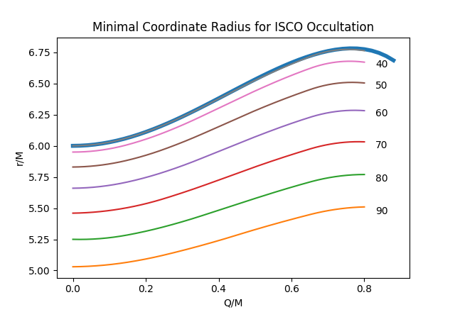
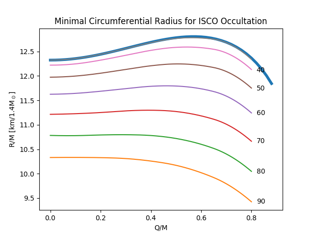
Figure 1: Minimal coordinate radius (upper panel) and circumferential radius (lower panel) for ISCO occultation by a NS as a function of the ratio of total scalar charge over the mass ($Q/M=0$ is GR), for various inclination of the observer with respect to the normal of the disk plane. The thick blue line is the ISCO radius as a function of the scalar charge.

In Fig. 2 we show the shape of the iron line for a viewing angle of $\psi=30^{\circ}$ in the absence of occultation, for various values of $Q/M$. It is intersting to note that the location of the edge at $\simeq 6.74$ keV does not depend on the presence of a scalar charge. On the other hand the effects of the scalar charge are more evident in the shape of the line. In particular, the intensity in the range $[5.9-6.6]$keV is smaller than in GR, from $\sim 2\%$ for $Q=0.3M$, to $\sim 7\%$ at $Q=0.8M$. For $Q>0.5M$ differences with respect to GR emerge also in the low energy tail. In particular we observe the formation of a second horn at $\simeq 5.6$keV, and a tail which is about $2\%$ brighter, and extends down to $3.2$keV, with respect to the low energy limit of $3.7$keV in GR.

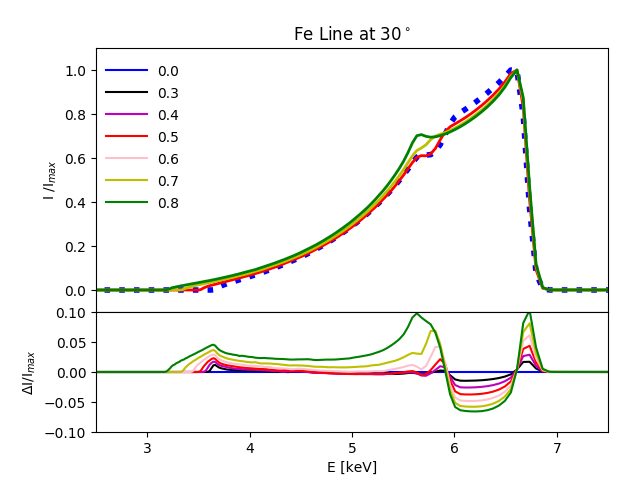
Figure 2: Upper panel: shape of the Fe K_α line, normalised to the maximum, for a viewing angle of $30^{\circ}$, and different values of the ratio of total scalar charge over the mass. The thick dotted blue line is the GR case. Lower panel: percentage deviation of the line shape as a function of the scalar charge with respect to GR.

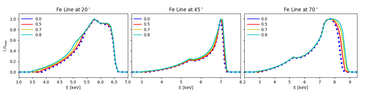
Figure 3: Shape of the Fe K_α line, normalised to the maximum, for various viewing angles ($20^{\circ}$ left, $45^{\circ}$ center, $70^{\circ}$ right), and different values of the ratio of total scalar charge over the mass. The thick dotted blue line is the GR case.

In Fig. 3 we show the shape of the iron line for various viewing angles, and for selected values of the scalar charge. It is evident that the way a scalar field modifies the line shape depends strongly on the viewing geometry. At $\psi=20^{\circ}$, the largest deviations are found in the intensity and shape of the low energy tail, and only partially in the shape of the $[6.0-6.5]$keV part. At $\psi=45^{\circ}$ instead the deviations are much smaller, while at $\psi=70^{\circ}$ they emerge again but now in the position of the high energy edge, which moves from $\simeq 8.2$keV to $\simeq 8.7$ keV, while the rest of the line shape is unaffected. The reason for this change with viewing angle is due to the fact that, for small viewing angles the shape of the line is mostly affected by gravitational redshift, and light bending, whose effects are more prominent in the low energy tails. This is where deviations from GR have the largest impact. On the other hand, when the inclination rises, and the disk is progressively seen more edge on, special relativistic effects due to orbital motion, and the related Doppler boosting, become dominant. The shape of the line now is more a tracer of the location and dynamics of the ISCO, which impacts mostly the high energy part of the line and the location of the edge. In general deviations in the intensity in the body of the line are small, at most few percent.

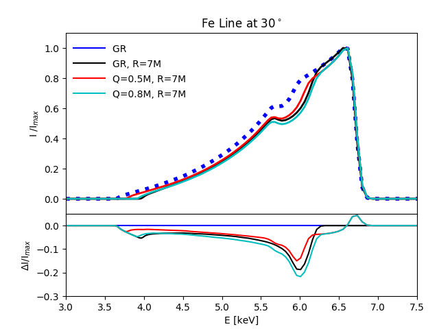
Figure 4: Shape of the Fe K_α line for $30^{\circ}$ viewing angle, and various values of the scalar charge and NS radius normalised to the maximum (thick dotted blue line is unocculted GR). Lower panel percentage deviation of the line shape as a function of the ratio of total scalar charge over the mass, with respect to unocculted GR.

In terms of occultation, for an observer inclination of $\psi=70^{\circ}$, the effect are small (less than few percent) and mostly concentrated in the low energy part of the line. However, when the NSs radius become larger than the ISCO (or in case the disk is truncated at radii larger than the ISCO radius), the high energy edge of the line begins to move to lower energy. For $Q=0.8M$ and $R=7M$ (greater than the ISCO radius for any $Q/M$) the leading edge is located at $\simeq 8.4$keV. For an observer inclination of $\psi=30^{\circ}$, when occultation does not take place, the effect of a NS that truncates the disk at radii larger than the ISCO, is mostly concentrated in the intermediate part of the line. Again the differences between the GR case, and STT are only few percents, as shown in Fig. 4.

4 Conclusions

In this work we have investigated how the space-time deviations produced by a non-minimally coupled scalar field, as hypothesised in some alternative theory of gravity, could be probed using the shape of the Fe K_α line in accreting NS systems. Given that STTs satisfy the Weak Equivalence Principle, standard ray tracing techniques of GR can easily be applied. The presence of a scalar field affects the shape of the line in two ways: on one hand, it changes the space-time, affecting the gravitational redshift and light bending; on the other, it modifies the Keplerian dynamics of matter orbiting in the disk, and the location of the ISCO, which leads to further deviations in the line shape associated to special relativistic Doppler boosting.

We found that such deviations however are at most a few percent, and only for large total scalar charges $Q>0.5M$. However, the typical luminosity of Low Mass X-ray Binaries, where the Fe line has been detected, is usually a sizeable fraction $0.05-0.11$ of the Eddington luminosity, and the intensity of the Fe line is typically 5-10% of the continuum. Given that the largest deviations from GR, in the line shape, extend over typical energy ranges $\sim 0.3-0.5$ keV, as can be seen, for example, from Fig. 2, and requiring the signal associated to these deviations to be well above ($S/N\sim 5$) the Poisson noise from the disk continuum (which, for isolated point-like sources, dominates the noise), in the same energy range, we can estimate the exposure time require to detect them. With the next generation of large collecting area X-ray satellites like ATHENA (whose expected effective area at 6 keV is $\simeq 2500$ cm², Barcons et al. 2017) we predict that deviations in the intensity of the line of the order of few percent could be detected with typical exposure times ranging from $10^{5}$s in the brightest sources like Sco X-1 e Ser X-1 to a few $10^{5}$s for weaker ones like 4U1608-52. More interesting is the fact that for large viewing angles, the high-energy edge can move enough to be revealed even with a low spectral resolution. This, in our opinion, could be the easiest deviation to measure.

There are of course several other issues, that can play a role in the correct modelling of the line shape (Miller, 2007; Dauser, García & Wilms, 2016). It is well known that the choice of the illuminator for example can affect it. The correct modelling of the background plays also a crucial role, as well as the presence of other lines that can blend (Iaria et al., 2009). Not to talk about the assumption of a disk truncated at the ISCO. It is also possible that scalarized NSs, having in general larger radii than in GR (Damour & Esposito-Farese, 1993), could lead to stronger occultation effects. However, even if this could provide an alternative way to measure the radius of the NS, it is not clear how degenerate the information it provides is with respect to the equation of state.

We stress again that this paper was organised as a proof of principle, and we opted for the simplest possible approach to test the viability of this effect. Given however the potential of this kind of measure as a possible independent test of GR and its alternatives, we deem that a more accurate evaluations of the expected results, considering specific STTs, or more realistic EoS, to account for the mutual relation between mass, scalar charge and NS radius, and specifically targeted to known systems, is worth a further analisys.

References

- Abramowicz & Kluźniak (2005) Abramowicz M. A., Kluźniak W., 2005, Ap&SS, 300, 127
- Anderson, Freire & Yunes (2019) Anderson D., Freire P., Yunes N., 2019, Classical and Quantum Gravity, 36, 225009
- Antoniadis et al. (2013) Antoniadis J. et al., 2013, Science, 340, 448
- Barcons et al. (2017) Barcons X. et al., 2017, Astronomische Nachrichten, 338, 153
- Barret et al. (2016) Barret D. et al., 2016, Society of Photo-Optical Instrumentation Engineers (SPIE) Conference Series, Vol. 9905, The Athena X-ray Integral Field Unit (X-IFU), p. 99052F
- Berti et al. (2015) Berti E. et al., 2015, Classical and Quantum Gravity, 32, 243001
- Brans & Dicke (1961) Brans C., Dicke R. H., 1961, Physical Review, 124, 925
- Cackett et al. (2008) Cackett E. M. et al., 2008, ApJ, 674, 415
- Capozziello & de Laurentis (2011) Capozziello S., de Laurentis M., 2011, Phys. Rep., 509, 167
- Coughenour et al. (2018) Coughenour B. M., Cackett E. M., Miller J. M., Ludlam R. M., 2018, ApJ, 867, 64
- Damour & Esposito-Farese (1993) Damour T., Esposito-Farese G., 1993, Phys. Rev. Lett., 70, 2220
- Dauser, García & Wilms (2016) Dauser T., García J., Wilms J., 2016, Astronomische Nachrichten, 337, 362
- Degenaar et al. (2015) Degenaar N., Miller J. M., Chakrabarty D., Harrison F. A., Kara E., Fabian A. C., 2015, MNRAS, 451, L85
- Demorest et al. (2010) Demorest P. B., Pennucci T., Ransom S. M., Roberts M. S. E., Hessels J. W. T., 2010, Nature, 467, 1081
- Doneva et al. (2014) Doneva D. D., Yazadjiev S. S., Stergioulas N., Kokkotas K. D., Athanasiadis T. M., 2014, Phys. Rev. D, 90, 044004
- Event Horizon Telescope Collaboration et al. (2019) Event Horizon Telescope Collaboration et al., 2019, ApJLett, 875, L1
- Fujii & Maeda (2003) Fujii Y., Maeda K.-I., 2003, The Scalar-Tensor Theory of Gravitation
- Ghasemi-Nodehi (2018) Ghasemi-Nodehi M., 2018, Phys. Rev. D, 97, 024043
- Hawking (1972) Hawking S. W., 1972, Communications in Mathematical Physics, 25, 167
- Homan et al. (2018) Homan J., Steiner J. F., Lin D., Fridriksson J. K., Remillard R. A., Miller J. M., Ludlam R. M., 2018, ApJ, 853, 157
- Iaria et al. (2009) Iaria R., D’Aí A., di Salvo T., Robba N. R., Riggio A., Papitto A., Burderi L., 2009, A&A, 505, 1143
- Just (1959) Just K., 1959, Zeitschrift Naturforschung Teil A, 14, 751
- Kammoun, Nardini & Risaliti (2018) Kammoun E. S., Nardini E., Risaliti G., 2018, A&A, 614, A44
- La Placa et al. (2020) La Placa R., Stella L., Papitto A., Bakala P., Di Salvo T., Falanga M., De Falco V., De Rosa A., 2020, arXiv e-prints, arXiv:2003.07659
- Laor (1991) Laor A., 1991, ApJ, 376, 90
- Matsuda & Nariai (1973) Matsuda T., Nariai H., 1973, Progress of Theoretical Physics, 49, 1195
- Matt et al. (1992) Matt G., Perola G. C., Piro L., Stella L., 1992, A&A, 257, 63
- Miller (2007) Miller J. M., 2007, ARA&A, 45, 441
- Nampalliwar et al. (2018) Nampalliwar S., Bambi C., Kokkotas K. D., Konoplya R. A., 2018, Physics Letters B, 781, 626
- Papantonopoulos (2015) Papantonopoulos E., 2015, Modifications of Einstein’s Theory of Gravity at Large Distances, Vol. 892
- Parker, Miller & Fabian (2018) Parker M. L., Miller J. M., Fabian A. C., 2018, MNRAS, 474, 1538
- Psaltis & Johannsen (2012) Psaltis D., Johannsen T., 2012, ApJ, 745, 1
- Risaliti et al. (2013) Risaliti G. et al., 2013, Nature, 494, 449
- Santiago & Silbergleit (2000) Santiago D. I., Silbergleit A. S., 2000, General Relativity and Gravitation, 32, 565
- Shao et al. (2017) Shao L., Sennett N., Buonanno A., Kramer M., Wex N., 2017, Physical Review X, 7, 041025
- Sotani (2017) Sotani H., 2017, Phys. Rev. D, 96, 104010
- Will (2014) Will C. M., 2014, Living Reviews in Relativity, 17, 4
- Yang, Ayzenberg & Bambi (2018) Yang J., Ayzenberg D., Bambi C., 2018, Phys. Rev. D, 98, 044024
- Yazadjiev, Doneva & Popchev (2016) Yazadjiev S. S., Doneva D. D., Popchev D., 2016, Phys. Rev. D, 93, 084038