Majorana molecules and their spectral fingerprints

Abstract

We introduce the concept of a Majorana molecule, a topological bound state appearing in the geometry of a double quantum dot (QD) structure flanking a topological superconducting nanowire. We demonstrate that, if the Majorana bound states (MBSs) at opposite edges are probed nonlocally in a two probe experiment, the spectral density of the system reveals the so-called half-bowtie profiles, while Andreev bound states (ABSs) become resolved into bonding and antibonding molecular configurations. We reveal that this effect is due to the Fano interference between pseudospin superconducting pairing channels and propose that it can be catched by a pseudospin resolved Scanning Tunneling Microscope (STM)-tip.

I Introduction

The recent decade witnessed the increasing interest of the condensed matter community in Majorana physics. In particular, the concept of Majorana bound states (MBSs) as promising building blocks for topologically protected and fault-tolerant quantum computing received special attention RAguado ; DasSarma ; JAlicea ; MFranz ; Chamon ; BTrauzettel . MBSs are zero-modes appearing at topological boundaries of condensed matter systems with spinless p-wave superconductivity, as it was first predicted by A. Y. Kitaev in his seminal work Kitaev . They manifest themselves via zero-bias peak (ZBP) signature in local conductance measurements Kouwenhoven1 . As candidates for hosting nonlocal MBSs, such material platforms as ferromagnetic atomic chains Beenaker ; Yazdani ; DLoss ; PSimon ; MFranz2 ; FVonOppen ; Yazdani2 ; Meyer ; Yazdani3 ; Franke ; Nitta and semiconductor hybrid nanowires Kouwenhoven1 ; Kouwenhoven2 ; CMarcus1 ; CMarcus2 ; CMarcus3 were proposed. Isolated MBSs are also supposed to be attached to cores of superconducting vortices Gao ; FuKane .

Interestingly enough, the Majorana quasiparticle detection can be done by determining transport quantities through a single quantum dot (QD) Baranger ; Vernek ; PabloSaoJose ; STMLDOS1 ; Noise0 ; Noise1 ; Noise2 ; Noise3 ; Thermo1 ; Thermo2 ; Thermo3 . As examples of such, we highlight the electrical shot-noise Noise0 ; Noise1 ; Noise2 ; Noise3 and the thermoelectric properties Thermo1 ; Thermo2 ; Thermo3 . Although the former cannot fully trace the QD density of states (DOS), it is specially helpful in introducing a full counting statistics of charge tunneling events, which is unique for Majorana systems Noise0 . Further, the shot-noise allows in distinguishing a nontopological ZBP from the corresponding topological Noise1 . It also reveals that the fractional value of the effective charge, by means of current fluctuations, thus depends on the system bias-voltage Noise2 . Additionally, the differential quantum noise shows that the photon absorbed spectra by a MBS shows a universal behavior, being frequency and bias-voltage independent Noise3 . Similarly, the zero-bias limit of the thermoelectric properties present striking features. The thermopower enhancement Thermo1 ; Thermo2 and according to some of us, the possibility of a tuner of heat and charge assisted by MBSs Thermo3 , are just few examples of such.

Astonishingly, upon attaching an extra QD, the control of the MBS leakage Vernek into QDs becomes feasible LeakingTwoDots1 ; LeakingTwoDots2 . According to Jesus D. Cifuentes et al. LeakingTwoDots1 , in several geometric arrangements of QDs, known as “parallel”, “in-series” and “T-shaped”, the spatial manipulation of a MBS is allowed. On the grounds of the pseudospin, this switching is revealed as the cornerstone for the Majorana fermion qubit cryptography, as proposed in Ref. LeakingTwoDots2 by some of us. This cryptography arises from the delicate interplay between Fano interference Fano ; ReviewFano and topological superconductivity.

Noteworthy, the pseudospin has been guided the interpretation of the transport through spinless two-level QD and double-QD systems Pseudo1 ; Pseudo2 ; Pseudo3 . Specially in the latter, the Kondo effect is induced by an interdot Coulomb correlation Pseudo3 . It is worth mentioning that, the pseudospin consists of mapping the system orbital degrees of freedom into those equivalent to the $z$-components of its spin $\frac{1}{2}$ counterpart, i.e., by projecting them along the quantization of the pseudospin axis Pseudo1 . We highlight that these peculiar degrees of freedom are experimentally detectable by the pseudospin resolved transport spectroscopy Pseudo4 .

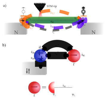
Figure 1: (Color online) (a) The sketch of the considered system with pseudospin resolved STM-tip acting as a probe of the one-dimensional topological superconductor (1D-TSC) and nonlocal Majorana bound states (MBSs) $\Psi_{j}=\Psi_{j}^{\dagger}$ ($j=1,2$) at the edges and flanked by a pair of QDs, with energies $\tilde{\varepsilon}_{L}$ and $\tilde{\varepsilon}_{R}$ coupled to metallic leads, via the hybridization $\mathcal{V}.$ The nonlocal MBSs couple to the QDs via the amplitudes $\lambda_{\alpha j}$ ($\alpha=L,R$) and to each other by the overlap term $\varepsilon_{M}.$ The system is characterized by spinless and p-wave superconductivity, due to the large Zeeman splitting. (b) Mapping of the original system into equivalent geometry with a single QD with pseudospin degrees of freedom. The amplitudes $\mathcal{V}_{\sigma}^{+}$ refer to the pseudospin pairing channels of the formation of Cooper pairs spatially split into the orbitals $(d_{\sigma}f)$ with energies $\varepsilon_{d\sigma}$ and $\varepsilon_{M}.$ The terms $\mathcal{V}_{\sigma}^{-}$ stand for pseudospin ballistic transport processes through such orbitals. The nonlocal orbital $f$ is formed by a pair of the MBSs.

Concerning the Fano interference in the presence of MBSs and QDs with a plethora of intriguing characteristics Recher ; Yokoyama ; Zhang ; Zheng ; Front ; Xiong ; Domanski ; Gong ; Orellana ; Seridonio1 , special attention should be paid to the findings of Ref. Zhang by J.-J. Xia et al.. Their results reveal that the conductance through two QDs obeys in an elegant manner, and within the low bias-voltage limit, a Fano-like expression Fano ; ReviewFano . Surprisingly, this expression is dressed by the QD-wire couplings and a Fano parameter of interference, which is dependent upon the MBSs overlapping. Therefore, such an analysis offers an attractive experimental strategy, clearly supported by the Fano effect, in recognizing MBSs far apart in superconducting wires, as well as in estimating how topological these MBSs are.

In this work, distinct from Refs. LeakingTwoDots1 ; LeakingTwoDots2 ; Zhang , by including the nonlocality degree of MBSs PabloSaoJose , we propose the concept of a Majorana molecule within the pseudospin framework Pseudo1 ; Pseudo2 ; Pseudo3 . It is worth citing that, such a nonlocality feature is a key ingredient for reproducing experimental results CMarcus3 ; PabloSaoJose . Then, this molecule appears in the configuration similar to those considered in the end of Ref. CMarcus3 , but with spectral fingerprints probed by a pseudospin resolved Scanning Tunneling Microscope (STM)-tip, similarly to Ref. STMLDOS1 and schematically shown in Fig.1(a) of the current paper. It consists of a one-dimensional (1D) topological superconductor (TSC) hosting MBSs at the edges, which hybridize with normal fermionic states of a pair of QDs flanking the TSC wire, placed in the strong longitudinal magnetic field. If the latter is strong enough, so that Zeeman splitting becomes much larger than all other characteristic energies of the system, the spinless condition is fulfilled. In this case, the tuning of the parameters of the system leads to a crossover between the well-known regime of individual Andreev bound states (ABSs) CMarcus3 (The Majorana molecule turned-off), and the regime in which one witnesses the splitting of the ABS into bonding and antibonding molecular configurations (The Majorana molecule turned-on). The formation of these states can be described in terms of the so-called pseudospins $(\uparrow,\downarrow)$, which determine the structure of the QDs orbitals by means of superconducting parings in these channels. Note that, contrary to the single QD geometry considered before CMarcus3 ; PabloSaoJose , in our setup the QDs act as a nonlocal two-probe detector which catches the Fano interference effects between various tunneling paths, including those involving the MBSs.

We demonstrate that, similar to what happens in the system of a pair of QDs placed within a semiconductor UsualMolecule or a Dirac-Weyl semimetal host Seridonio2 ; Seridonio3 , the Fano effect in the considered system defines the novel type of molecular binding of QD orbitals, and leads to the formation of a Majorana molecule, characterized by the so-called half-bowtie profiles in the spectral density of states.

II The Model

The geometry we consider is shown in the Fig.1(a). The system under study consists of an STM-tip perturbatively coupled to the 1D-TSC nanowire with nonlocal MBSs formed at its edges and flanked by a pair of QDs, where the latter are attached to metallic leads. We suggest that the external magnetic field applied along the direction of the wire is large enough, so that only spin up states lie below the Fermi energy, and spin down states can be just totally excluded from the consideration Thermo3 ; Baranger ; Vernek . We account for the possible coupling between MBSs localized at the opposite edges of the TSC wire, which can change their nonlocality degree and lead to the crossover between highly nonlocal MBSs and more local ABSs.

The Hamiltonian of the system reads:

$$\mathcal{H} = \sum_{\alpha\mathbf{k}}\varepsilon_{\alpha\mathbf{k}}\tilde{c}_{\alpha\mathbf{k}}^{\dagger}\tilde{c}_{\alpha\mathbf{k}}+\sum_{\alpha}\tilde{\varepsilon}_{\alpha}\tilde{d}_{\alpha}^{\dagger}\tilde{d}_{\alpha}+t_{\text{{c}}}(\tilde{d}_{L}^{\dagger}\tilde{d}_{R}+\text{{H.c.}})$$ (1)

$$+ \mathcal{V}\sum_{\alpha\mathbf{k}}(\tilde{c}_{\alpha\mathbf{k}}^{\dagger}\tilde{d}_{\alpha}+\text{{H.c.}})+\lambda_{L1}(\tilde{d}_{L}-\tilde{d}_{L}^{\dagger})\Psi_{1}$$

$$+ i\lambda_{L2}(\tilde{d}_{L}+\tilde{d}_{L}^{\dagger})\Psi_{2}+i\lambda_{R1}(\tilde{d}_{R}+\tilde{d}_{R}^{\dagger})\Psi_{2}$$

$$+ \lambda_{R2}(\tilde{d}_{R}-\tilde{d}_{R}^{\dagger})\Psi_{1}+i\varepsilon_{M}\Psi_{1}\Psi_{2},$$

where the operators $\tilde{c}_{\alpha\mathbf{k}}^{\dagger},\tilde{c}_{\alpha\mathbf{k}}$ correspond to electrons in the right and left metallic leads $\alpha=L,R$ having momentum $\mathbf{k}$ and energy $\varepsilon_{\alpha\mathbf{k}}=\varepsilon_{\mathbf{k}}-\mu_{\alpha},$ with $\mu_{\alpha}$ the corresponding chemical potential. The operators $\tilde{d}_{\alpha}^{\dagger},\tilde{d}_{\alpha}$ describe the localized orbitals in the right and left QDs with energies $\tilde{\varepsilon}_{\alpha}$, $t_{\text{{c}}}$ is the hopping term corresponding to the normal direct tunneling between the QDs, which can lead to the formation of usual molecular orbitals UsualMolecule and $\mathcal{V}$ describes the strength of the coupling between the QDs and the leads (we take it equal for right and left QDs). At the edges of the TSC wire, the nonlocal MBSs described by the operators $\Psi_{j}=\Psi_{j}^{\dagger}$, couple to the QDs with the amplitudes $\lambda_{\alpha j}$ with $j=1,2$ (the ratio $\eta_{\alpha}=|\lambda_{\alpha 1}/\lambda_{\alpha 2}|$ defines the nonlocality degree) and to each other via the overlap term $\varepsilon_{M}.$

Linear combination of the Majorana operators

$$f=\frac{1}{\sqrt{2}}(\Psi_{1}+i\Psi_{2})$$ (2)

forms a regular fermionic state.

Performing the rotation in the pseudospin space $\sigma=\pm 1$ $(\uparrow,\downarrow),$ with the two leads at the same chemical potential $\mu_{L}=\mu_{R}=0$ Pseudo3 , corresponding to R and L states, $\tilde{d}_{L}=\cos\theta d_{\uparrow}-\sin\theta d_{\downarrow}$, $\tilde{d}_{R}=\sin\theta d_{\uparrow}+\cos\theta d_{\downarrow}$, $\tilde{c}_{\mathbf{k}L}=\cos\theta c_{\mathbf{k}\uparrow}-\sin\theta c_{\mathbf{k}\downarrow}$, $\tilde{c}_{\mathbf{k}R}=\sin\theta c_{\mathbf{k}\uparrow}+\cos\theta c_{\mathbf{k}\downarrow}$ with

$$\theta=\frac{\pi}{4}+\frac{1}{2}\arcsin\frac{\triangle\varepsilon}{\sqrt{4(t_{\text{{c}}})^{2}+(\triangle\varepsilon)^{2}}}$$ (3)

and $\triangle\varepsilon=\tilde{\varepsilon}_{L}-\tilde{\varepsilon}_{R},$ the Hamiltonian of the system can be rewritten as:

$$\mathcal{H} = \sum_{\mathbf{k}\sigma}\varepsilon_{\mathbf{k}}c_{\mathbf{k}\sigma}^{\dagger}c_{\mathbf{k}\sigma}+\sum_{\sigma}\varepsilon_{d\sigma}d_{\sigma}^{\dagger}d_{\sigma}+\mathcal{V}\sum_{\mathbf{k}\sigma}(c_{\mathbf{k}\sigma}^{\dagger}d_{\sigma}+\text{{H.c.}})$$ (4)

$$+ \varepsilon_{M}(f^{\dagger}f-\frac{1}{2})+\sum_{\sigma}(\mathcal{V}_{\sigma}^{-}d_{\sigma}f^{\dagger}+\mathcal{V}_{\sigma}^{+}d_{\sigma}f+\text{{H.c.}}),$$

where $\varepsilon_{d\sigma}=\frac{(\tilde{\varepsilon}_{L}+\tilde{\varepsilon}_{R})}{2}-\frac{\sigma}{2}\sqrt{4(t_{\text{{c}}})^{2}+(\triangle\varepsilon)^{2}},$ $\mathcal{V}_{\uparrow}^{\mp}=\frac{1}{\sqrt{2}}[(\lambda_{R2}\mp\lambda_{R1})\sin\text{$\theta$}+(\lambda_{L1}\mp\lambda_{L2})\cos\theta]$ and $\mathcal{V}_{\downarrow}^{\mp}=\frac{1}{\sqrt{2}}[(\lambda_{R2}\mp\lambda_{R1})\cos\text{$\theta$}-(\lambda_{L1}\mp\lambda_{L2})\sin\theta].$

The Hamiltonian given by Eq. (4) corresponds to the mapping of the original problem to one equivalent to a single spinor QD coupled to fermionic state $f$ and characterized by the following mixture of states: the amplitudes $\mathcal{V}_{\uparrow(\downarrow)}^{+}$ correspond to the formation of delocalized Cooper pairs $(d_{\sigma}f)$, while the terms $\mathcal{V}_{\uparrow(\downarrow)}^{-}$ give the normal couplings between the effective QD and $f$ ($d_{\sigma}f^{\dagger}$).

By making explicit the pseudospin basis, we recognize the symmetric $d_{\uparrow}=\sin\theta\tilde{d}_{R}+\cos\theta\tilde{d}_{L}$ and antisymmetric $d_{\downarrow}=\cos\theta\tilde{d}_{R}-\sin\theta\tilde{d}_{L}$ superpositions as the bonding and antibonding molecular states, respectively, due to the linear combination of atomic orbitals (LCAO) between $\tilde{d}_{L}$ and $\tilde{d}_{R}.$ Strictly for $t_{c}=0,$ note that from Eq.(3), $\theta=\frac{\pi}{2}$($\theta=0$) when $\Delta\varepsilon\rightarrow 0^{+}$($\Delta\varepsilon\rightarrow 0^{-}$) leading to the breaking down of the LCAO. As we are interested in the pairing dominated by the MBSs, in the following discussion, we will consider then the case of identical QDs weakly coupled. It corresponds to $\tilde{\varepsilon}_{L}=\tilde{\varepsilon}_{R}=\varepsilon_{d}$ and $t_{c}\rightarrow 0$, but finite as in Ref.Hoppingtc , thus giving rise to $\theta=\frac{\pi}{4}$ as shown in Fig.2(a) of Sec. III, where we present the profile of Eq.(3) as a function of $\Delta\varepsilon$ for several $t_{c}$ values.

The QD states corresponding to the opposite pseudospins are now simply symmetric and antisymmetric combinations between the orbitals of right and left QDs:

$$d_{\uparrow}=\frac{\tilde{d}_{R}+\tilde{d}_{L}}{\sqrt{2}}\,\,\,\text{and}\,\,\,d_{\downarrow}=\frac{\tilde{d}_{R}-\tilde{d}_{L}}{\sqrt{2}},$$ (5)

which represent the bonding and antibonding molecular states with the energies $\varepsilon_{d\sigma}=\varepsilon_{d}-\sigma t_{c}$, respectively. Moreover,

$$\mathcal{V}_{\uparrow}^{\mp}=\frac{\lambda_{R2}+\lambda_{L1}\mp(\lambda_{R1}+\lambda_{L2})}{2}$$ (6)

and

$$\mathcal{V}_{\downarrow}^{\mp}=\frac{\lambda_{R2}-\lambda_{L1}\mp(\lambda_{R1}-\lambda_{L2})}{2}.$$ (7)

As we will see, the communication between the QDs lead to the splitting of the ABSs into ABS-$\uparrow$ and ABS-$\downarrow$, and formation of a Majorana molecule.

We characterize the QDs by their normalized spectral densities

$$\tau{}_{jl}\left(\omega\right)=-\Gamma\text{{Im}}(\langle\langle d_{j};d_{l}^{\dagger}\rangle\rangle),$$ (8)

where $j,l=L,R$, $\langle\langle d_{j};d_{l}^{\dagger}\rangle\rangle$ are retarded Green’s functions (GFs) in the frequency domain and $\Gamma=\pi\mathcal{V}^{2}\sum_{\mathbf{k}}\delta(\varepsilon-\varepsilon_{\mathbf{k}})$ Anderson . We highlight that Eq.(8) is temperature independent, once in the system Hamiltonian of Eq.(1) the Coulomb correlation $U\tilde{d}_{L}^{\dagger}\tilde{d}_{L}\tilde{d}_{R}^{\dagger}\tilde{d}_{R},$ which corresponds to $Ud_{\uparrow}^{\dagger}d_{\uparrow}d_{\downarrow}^{\dagger}d_{\downarrow}$ in Eq.(4), is suppressed by the superconducting wire between the QDs, as discussed in Ref. Hoppingtc . Otherwise, the interdot correlation would induce the Kondo effect Pseudo3 . Performing the pseudospin rotation given by Eq. (5), we get

$$\tau_{LL(RR)}\left(\omega\right)=\frac{1}{2}\{(\tau_{\uparrow\uparrow}+\tau_{\downarrow\downarrow})\mp(\tau_{\uparrow\downarrow}+\tau_{\downarrow\uparrow})\}$$ (9)

and

$$\tau_{RL(LR)}\left(\omega\right)=\frac{1}{2}\{(\tau_{\uparrow\uparrow}-\tau_{\downarrow\downarrow})\mp(\tau_{\uparrow\downarrow}-\tau_{\downarrow\uparrow})\}$$ (10)

for the local and nonlocal QDs densities, respectively. The presence of the terms $\tau_{\uparrow\downarrow}(\tau_{\downarrow\uparrow})$ accounts for the Fano interference in the pseudospin channels. Conversely, the QDs $\tilde{d}_{L}$ and $\tilde{d}_{R}$ interfere to each other, thus forming $\tau_{\uparrow\uparrow}\left(\omega\right)$ (bonding) and $\tau_{\downarrow\downarrow}\left(\omega\right)$ (antibonding) orbitals

$$\tau_{\uparrow\uparrow(\downarrow\downarrow)}\left(\omega\right)=\frac{1}{2}\{(\tau_{LL}+\tau_{RR})\pm(\tau_{RL}+\tau_{LR})\}$$ (11)

and

$$\tau_{\uparrow\downarrow(\downarrow\uparrow)}\left(\omega\right)=\frac{1}{2}\{(\tau_{RR}-\tau_{LL})\pm(\tau_{LR}-\tau_{RL})\}.$$ (12)

As the left and right metallic leads should have the same chemical potentials ($\mu_{L}=\mu_{R}=0$ Pseudo3 ) for the emergence of the pseudospin scenario of Eq.(4), the differential conductance $\mathcal{G}$ at a finite bias-voltage $eV$ cannot be measured through these leads. Thus, the experimental detection of the spectral densities given by Eqs.(9) and (11) needs an extra electron reservoir. To that end, the transport can be observed by employing an STM-tip perturbatively coupled to the 1D-TSC and QDs, as proposed in Fig.1(a) and Ref.STMLDOS1 . In such an apparatus, by considering the temperature $T\rightarrow 0\text{{K}}$ ($k_{\text{{B}}}T\ll\Gamma$, where $k_{\text{{B}}}$ is the Boltzmann constant and $\Gamma=40\mu eV$ Vernek as the system energy scale) and low bias-voltage $eV\rightarrow 0$ ($eV\ll\Gamma$), $\mathcal{G}\propto\int d\omega\text{{LDOS}}(\omega)\left\{-\frac{\partial}{\partial\varepsilon}n_{F}(\omega-eV)\right\}\approx\text{{LDOS}}(eV),$ with $n_{F}$ as the Fermi-Dirac distribution and $\left\{-\frac{\partial}{\partial\varepsilon}n_{F}(\omega-eV)\right\}\approx\delta(\omega-eV).$ This means that the conductance becomes ruled by the Local Density of States (LDOS) evaluated at the tip chemical potential $\mu_{\text{{tip}}}=eV=\omega.$ For the STM-tip placed over the left (right) QD, the LDOS behavior will be determined by $\tau_{LL}\left(\omega\right)$ ($\tau_{RR}\left(\omega\right)$), but upon varying the tip position over the wire, the LDOS is expected to catch traces of the interfering processes through the QDs, such as those present in $\tau_{\uparrow\uparrow}\left(\omega\right)$ Seridonio2 ; Seridonio3 . By this manner, the STM-tip becomes naturally pseudospin resolved. Noteworthy, we clarify that the quantitative evaluation of the LDOS spatial dependence along the 1D-TSC is not the focus of the current work, once it requires to adopt the Kitaev chain explicitly in the approach.

To evaluate $\langle\langle d_{\sigma};d_{\sigma^{\prime}}^{\dagger}\rangle\rangle,$ we apply the equation-of-motion method FlensbergBook to Eq.(4), which gives:

$$(\omega+i0^{+})\langle\langle d_{\sigma};d_{\sigma^{\prime}}^{\dagger}\rangle\rangle=\delta_{\sigma\sigma^{\prime}}+\langle\langle\left[d_{\sigma},\mathcal{\mathcal{H}}\right];d_{\sigma^{\prime}}^{\dagger}\rangle\rangle.$$ (13)

The last term in the Eq.(13) will generate the anomalous Green functions $\langle\langle d_{\sigma}^{\dagger};d_{\sigma^{\prime}}^{\dagger}\rangle\rangle$. As the Hamiltonian is quadratic, the system of equations can be closed and written in the matrix form as $\bm{A}^{\sigma}\left(\omega\right)(\begin{array}[]{cccc}\langle\langle d_{\sigma};d_{\sigma}^{\dagger}\rangle\rangle&\langle\langle d_{\bar{\sigma}};d_{\sigma}^{\dagger}\rangle\rangle&\langle\langle d_{\sigma}^{\dagger};d_{\sigma}^{\dagger}\rangle\rangle&\langle\langle d_{\bar{\sigma}}^{\dagger};d_{\sigma}^{\dagger}\rangle\rangle)^{T}\end{array}=\begin{array}[]{cccc}(1&0&0&0\end{array})^{T},$ with

$$\bm{A}^{\sigma}\left(\omega\right)=\left[\begin{array}[]{cccc}a_{\sigma}\left(\omega\right)&-k_{2-}^{\sigma\bar{\sigma}}\left(\omega\right)&k_{1-}^{\sigma\sigma}\left(\omega\right)&k_{1-}^{\sigma\bar{\sigma}}\left(\omega\right)\\ -k_{2-}^{\bar{\sigma}\sigma}\left(\omega\right)&a_{\bar{\sigma}}\left(\omega\right)&k_{1-}^{\bar{\sigma}\sigma}\left(\omega\right)&k_{1-}^{\bar{\sigma}\bar{\sigma}}\left(\omega\right)\\ k_{1+}^{\sigma\sigma}\left(\omega\right)&k_{1+}^{\sigma\bar{\sigma}}\left(\omega\right)&b_{\sigma}\left(\omega\right)&-k_{2+}^{\sigma\bar{\sigma}}\left(\omega\right)\\ k_{1+}^{\bar{\sigma}\sigma}\left(\omega\right)&k_{1+}^{\bar{\sigma}\bar{\sigma}}\left(\omega\right)&-k_{2+}^{\bar{\sigma}\sigma}\left(\omega\right)&b_{\bar{\sigma}}\left(\omega\right)\end{array}\right],$$ (18)

where $\bar{\sigma}=-\sigma$,$k_{1\mp}^{\sigma\sigma^{\prime}}\left(\omega\right)=\mathcal{V}_{\sigma}^{-}\mathcal{V}_{\sigma^{\prime}}^{+}(\omega\mp\varepsilon_{M})^{-1}+\mathcal{V}_{\sigma^{\prime}}^{-}\mathcal{V}_{\sigma}^{+}(\omega\pm\varepsilon_{M})^{-1},$$k_{2\mp}^{\sigma\sigma^{\prime}}\left(\omega\right)=\mathcal{V}_{\sigma}^{-}\mathcal{V}_{\sigma^{\prime}}^{-}(\omega\mp\varepsilon_{M})^{-1}+\mathcal{V}_{\sigma}^{+}\mathcal{V}_{\sigma^{\prime}}^{+}(\omega\pm\varepsilon_{M})^{-1},$ $a_{\sigma}\left(\omega\right)=\omega-\varepsilon_{d\sigma}-k_{2-}^{\sigma\sigma}+i\Gamma$ and $b_{\sigma}\left(\omega\right)=\omega+\varepsilon_{d\sigma}-k_{2+}^{\sigma\sigma}+i\Gamma.$

III Results and Discussion

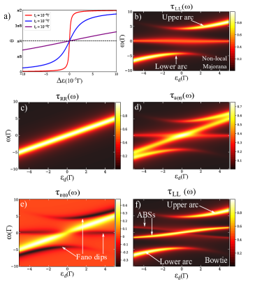
Figure 2: (Color online) The Majorana molecule turned-off scenario. Color maps of the spectral density of the QDs spanned by $\omega$ and $\varepsilon_{d}=\tilde{\varepsilon}_{L}=\tilde{\varepsilon}_{R}$. Panel (a) shows Eq.(3) for $\theta$ as function of $\triangle\varepsilon,$ which points out that for two identical weakly coupled QDs ($t_{c}\rightarrow 0,$ but finite as in Ref.Hoppingtc ), Eq.(4) should be evaluated at $\theta=\frac{\pi}{4}.$ Panels (b)-(e) correspond to the case of a right QD weakly coupled to the MBSs, $\lambda_{L1}=3\Gamma$ and $t_{c}=\lambda_{L2}=\lambda_{R1}=\lambda_{R2}=\varepsilon_{M}=10^{-5}\Gamma$. In panel (b) the density plot of $\tau_{LL}(\omega)$ demonstrates clearly visible horizontal bright line, corresponding to the ZBP due to the coupling with the MBS $\Psi_{1},$ which is robust against changes in $\varepsilon_{d}$ Vernek . In panel (c) the spectral density $\tau_{RR}\left(\omega\right)$ reveals solely the resonant level of the right QD, weakly coupled to the MBSs at $\omega=\varepsilon_{d}$. In this regime, Fano interference between the QDs is absent and $\tau_{RL}\left(\omega\right)=\tau_{LR}\left(\omega\right)=0.$ Panels (d) and (e) show $\tau_{\uparrow\uparrow}\left(\omega\right)=\tau_{\downarrow\downarrow}\left(\omega\right)$, and $\tau_{\uparrow\downarrow}\left(\omega\right)=\tau_{\downarrow\uparrow}\left(\omega\right)$ respectively, which reveal clear signatures of constructive and destructive Fano interference. Panel (f) accounts for the coupling of the left QD to the overlapping MBSs ($\lambda_{L1}=3\Gamma,$ $\lambda_{L2}=0.001\Gamma,$ $t_{c}=\lambda_{R1}=\lambda_{R2}=10^{-5}\Gamma$ and $\varepsilon_{M}=2\Gamma$). In this case the density plot for $\tau_{LL}$ reveals the transformation of the horizontal bright line, corresponding to the ZBP, into a bowtie profile, characteristic for split ABSs CMarcus3 .

We assume $\Gamma=40\mu eV$ Vernek as the energy scale of the model parameters of the system. In Fig.2(a) we present Eq.(3) as a function of $\triangle\varepsilon,$ which shows that the pseudospin mapping is applied to $\theta=\frac{\pi}{4},$ when $t_{c}\rightarrow 0$, but finite for the experimental condition $\triangle\varepsilon=0.$ This point defines the scenario adopted in this work for the evaluation of the spectral analysis.

Our aim is to investigate the spectral function of the considered system defined by the Eq. (8). To better understand the situation qualitatively, we start from the geometry wherein only the left QD is strongly coupled to MBSs, i.e, from the Majorana molecule turned-off scenario. We present the results for both the case of highly nonlocal MBS Vernek (Fig.2(b)) and the case of overlapping MBSs (Fig.2(f)). For both cases we present the 2D plots of the spectral functions in the $\omega$ and $\varepsilon_{d}$ axes.

Fig.2(b) shows the spectral function corresponding to the left QD, $\tau_{LL}\left(\omega\right)$ in the situation, when it is strongly coupled only to the closest MBS ($\lambda_{L1}=3\Gamma$ and $t_{c}=\lambda_{R1}=\lambda_{R2}=\lambda_{L2}=\varepsilon_{M}=10^{-5}\Gamma$). In perfect agreement with the Ref.Vernek , one can see the bright plateau at $\omega=0$, corresponding to the ZBP in the conductance, which is robust against the $\varepsilon_{d}$ perturbations and is provided by the presence of highly nonlocal MBSs. The upper and lower arcs correspond to the QD states split by the coupling to the MBS $\Psi_{1}.$ Naturally, as the right QD is weakly coupled to both MBSs, its spectral function $\tau_{RR}\left(\omega\right)$, shown in the Fig.2(c) is trivial and consists of a single peak corresponding to $\omega=\varepsilon_{d}.$ As the QDs do not communicate through the 1D-TSC, $\tau_{RL}\left(\omega\right)=\tau_{LR}\left(\omega\right)=0$.

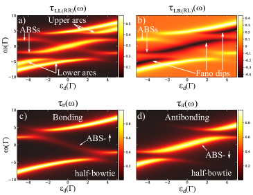
Figure 3: (Color online) The Majorana molecule turned-on scenario. Color maps of the spectral density of the QDs spanned by $\omega$ and $\varepsilon_{d}=\tilde{\varepsilon}_{L}=\tilde{\varepsilon}_{R}$. The parameters of the system are $t_{c}=10^{-5}\Gamma,$ $\lambda_{L1}=\lambda_{R1}=3\Gamma,$ $\lambda_{L2}=\lambda_{R2}=1.5\Gamma$ and $\varepsilon_{M}=0.05\Gamma$. Panel (a) shows the profiles of $\tau_{LL}(\omega)=\tau_{RR}(\omega)$, and reveals the splitting of the upper and lower arcs due to the formation of the bonding (ABS-$\uparrow$) and antibonding (ABS-$\downarrow$) Andreev molecular states. The pseudospin lifting in $\tau_{\uparrow\uparrow(\downarrow\downarrow)}\left(\omega\right)$ is attributed to the Fano interference between $\tau_{LL(RR)}\left(\omega\right)$ and $\tau_{LR(RL)}\left(\omega\right)$, which appears in panel (b). Formation of the aforementioned molecular states is even more clearly visible in the panels (c) and (d), corresponding to $\tau_{\uparrow\uparrow}\left(\omega\right)$ and $\tau_{\downarrow\downarrow}\left(\omega\right)$, where at the novel half-bowtie-like structures are formed. In this regime $\tau_{\uparrow\downarrow}\left(\omega\right)=\tau_{\downarrow\uparrow}\left(\omega\right)=0$, and Majorana molecular states are resolved in the pseudospin basis.

In the pseudospin basis, the latter condition, according to the Eqs.(6,7,11,12), imposes the pseudospin degeneracy, so that $\tau_{\uparrow\uparrow}\left(\omega\right)=\tau_{\downarrow\downarrow}\left(\omega\right)$ (shown in the Fig.2(d)), and $\tau_{\downarrow\uparrow}\left(\omega\right)=\tau_{\uparrow\downarrow}\left(\omega\right)$ (Fig.2(e)), $|\mathcal{V}_{\uparrow}^{-}|=|\mathcal{V}_{\downarrow}^{-}|$ and $|\mathcal{V}_{\uparrow}^{+}|=|\mathcal{V}_{\downarrow}^{+}|$, and, besides, $|\mathcal{V}_{\sigma}^{-}|=|\mathcal{V}_{\sigma}^{+}|$. Pseudospin degeneracy, in particular, means that, both Cooper pairings in the pseudospin channels given by $d_{\uparrow}f$ and $d_{\downarrow}f$ contribute to the Hamiltonian on the equal footing. The fact, that $\tau_{\downarrow\uparrow(\uparrow\downarrow)}\left(\omega\right)\neq 0$ means, that two pseudospin channels, corresponding to bonding and antibonding states, are non-orthogonal, and thus Majorana molecule is not formed. Spectral functions in the pseudospin basis are presented in the Figs.2(d)-(e), and reveal clear signatures of the Fano interference peaks and dips.

If one accounts for the coupling of the left QD to the MBS $\Psi_{2}$ ($\lambda_{L2}=0.001\Gamma$), with finite overlap between the states $\Psi_{1}$ and $\Psi_{2}$ ($\varepsilon_{M}=2\Gamma$), but keeps right QD weakly coupled ($t_{c}=\lambda_{R1}=\lambda_{R2}=10^{-5}\Gamma$), the spectral function $\tau_{LL}\left(\omega\right)$ reveals characteristic bowtie profile CMarcus3 ; PabloSaoJose (also referred as double fork Thermo3 ) instead of a robust ZBP. This corresponds to the presence in the system of a pair of trivial ABSs, as it is shown in the Fig.2(f). Other spectral functions remain qualitatively the same. The condition of pseudospin degeneracy still holds and a Majorana molecule is not formed.

Now, we can consider the symmetric case sketched in Fig.1(a) with $t_{c}=10^{-5}\Gamma,$ $\lambda_{L1}=\lambda_{R1}=3\Gamma,$ $\lambda_{L2}=\lambda_{R2}=1.5\Gamma$ and $\varepsilon_{M}=0.05\Gamma,$ corresponding to The Majorana molecule turned-on scenario: both QDs are coupled to both MBSs, and thus interfere with each other through the 1D-TSC. In this situation, a bowtie-like signature emerges in the spectral density $\tau_{LL(RR)}\left(\omega\right)$, as it can be seen from Fig. 3(a). Moreover, the features characteristic to usual molecular binding can be seen, as upper and lower arcs provided by the coupling of the QD states, visible in Fig. 2(f), become split in Fig. 3(a) due to the TSC-mediated overlap of the states of right and left QDs. Naturally, this leads to $\tau_{RL}\left(\omega\right)=\tau_{LR}\left(\omega\right)\neq 0$ (see Fig. 3(b)), which, according to the Eqs. (11) and (12) means that $\tau_{\uparrow\uparrow}\left(\omega\right)\neq\tau_{\downarrow\downarrow}$ and $\tau_{\downarrow\uparrow(\uparrow\downarrow)}\left(\omega\right)=0$.

Physically, this means that spin up and spin down channels become decoupled in the pseudospin basis and a Majorana molecule, which is a bonding or antibonding superposition of ABSs is formed. The latter manifest themselves in the spectral profiles of $\tau_{\uparrow\uparrow}(\omega)$ and $\tau_{\downarrow\downarrow}(\omega)$ shown in Figs.3(c) and (d), respectively as half-bowtie signatures. They are consequences of the Fano interference between $\tau_{LR}(\omega)$ and $\tau_{RL}(\omega)$, shown in Fig.3(b). Note that the latter contains both peaks and pronounced Fano dips, which interfere constructively or destructively depending on the sign in the Eqs. (11) and (12), with the peaks in the spectral densities of $\tau_{LL}(\omega)$ and $\tau_{RR}(\omega)$, which gives in the end the mentioned half-bowtie profiles.

In terms of the effective Hamiltonian [Eq. (4)], the considered regime corresponds to the case when $|\mathcal{V}_{\downarrow}^{-}|\neq 0,$ $|\mathcal{V}_{\uparrow}^{-}|=0$, $|\mathcal{V}_{\downarrow}^{+}|=0$ and $|\mathcal{V}_{\uparrow}^{+}|\neq 0$. This means that only the pseudospin Cooper pairing $d_{\uparrow}f$ and normal electron tunneling $d_{\downarrow}f^{\dagger}$ contribute to the transport assisted by the formation of Majorana molecules.

IV Conclusions

In summary, we have proposed the concept of a Majorana molecule, a bonding or antibonding state appearing in the system of a pair of QDs flanking a 1D-TSC nanowire. The coupling between QDs is achieved via the channel provided by the presence of MBSs. It is demonstrated that these states manifest themselves via half-bowtie spectral fingerprints in the spectral density of states, which are qualitatively different from full bowtie profiles, characteristic to the case of a single QD. Such features can be measured by an STM-tip, which becomes naturally pseudospin resolved, once the QDs behave as a nonlocal two-probe detector of the Fano interference assisted by the MBSs.

V Acknowledgments

We thank the Brazilian funding agencies CNPq (Grants No. 305668/2018-8 and No. 302498/2017-6), the São Paulo Research Foundation (FAPESP; Grant No. 2015/23539-8) and Coordenação de Aperfeiçoamento de Pessoal de Nível Superior – Brasil (CAPES) – Finance Code 001. Y.M. and I.A.S. acknowledge support from the Government of the Russian Federation through the Megagrant 14.Y26.31.0015, and ITMO 5-100 Program.

References

- (1) R. Aguado, Riv. Nuovo Cimento 40, 523 (2017).
- (2) C. Nayak, S. H. Simon, A. Stern, M. Freedman, and S. Das Sarma, Rev. Mod. Phys. 80, 1083 (2008).
- (3) J. Alicea, Rep. Prog. Phys. 75, 076501 (2012).
- (4) S. R. Elliott and M. Franz, Rev. Mod. Phys. 87, 137 (2015).
- (5) G. Goldstein and C. Chamon, Phys. Rev. B 84, 205109 (2011).
- (6) J. C. Budich, S. Walter, and B. Trauzettel, Phys. Rev. B 85, 121405(R) (2012).
- (7) A. Y. Kitaev, Phys. Usp. 44, 131 (2001).
- (8) H. Zhang, C.-X. Liu, S. Gazibegovic, D. Xu, J. A. Logan, G. Wang, N. van Loo, J. D. S. Bommer, M. W. A. de Moor, D. Car, R. L. M. Op het Veld, P. J. van Veldhoven, S. Koelling, M. A. Verheijen, M. Pendharkar, D. J. Pennachio, B. Shojaei, J. S. Lee, C. J. Palmstrom, E. P. A. M. Bakkers, S. D. Sarma, and L. P. Kouwenhoven, Nature (London) 556, 74 (2018).
- (9) T.-P. Choy, J.M. Edge, A.R. Akhmerov, C.W.J. Beenakker, Phys. Rev. B 84, 195442 (2011).
- (10) S. Nadj-Perge, I.K. Drozdov, B.A. Bernevig, A. Yazdani, Phys. Rev. B 88, 020407 (2013).
- (11) J. Klinovaja, P. Stano, A. Yazdani, D. Loss, Phys. Rev. Lett. 111, 186805 (2013).
- (12) B. Braunecker, P. Simon, Phys. Rev. Lett. 111, 147202 (2013).
- (13) M.M. Vazifeh, M. Franz, Phys. Rev. Lett. 111, 206802 (2013).
- (14) F. Pientka, L.I. Glazman, F. von Oppen, Phys. Rev. B 88, 155420 (2013).
- (15) S. Nadj-Perge, I.K. Drozdov, J. Li, H. Chen, S. Jeon, J. Seo, A.H. MacDonald, B.A. Bernevig, A. Yazdani, Science 346, 602 (2014).
- (16) R. Pawlak, M. Kisiel, J. Klinovaja, T. Meier, S. Kawai, T. Glatzel, D. Loss, E. Meyer, Quantum Inf. 2, 16035 (2016).
- (17) S. Jeon, Y. Xie, J. Li, Z. Wang, B.A. Bernevig, A. Yazdani, Science 358, 772 (2017).
- (18) M. Ruby, B.W. Heinrich, Y. Peng, F. von Oppen, K.J. Franke, Nano Lett. 17, 4473 (2017).
- (19) P. Marra, M. Nitta, Phys. Rev. B 100, 220502 (2019).
- (20) V. Mourik, K. Zuo, S. M. Frolov, S. R. Plissard, E. P. A. M. Bakkers, and L. P. , Science 336, 1003 (2012).
- (21) S. M. Albrecht, A. Higginbotham, M. Madsen, F. Kuemmeth, T. S. Jespersen, J. Nygard, P. Krogstrup, and C. Marcus, Nature (London) 531, 206 (2016).
- (22) M.-T. Deng, S. Vaitiekėnas, E. B. Hansen, J. Danon, M. Leijnse, K. Flensberg, J. Nygard, P. Krogstrup, and C. M. Marcus, Science 354, 1557 (2016).
- (23) M.-T. Deng, S. Vaitiekėnas, E. Prada, P. San-Jose, J. Nygard, P. Krogstrup, R. Aguado, and C. M. Marcus, Phys. Rev. B 98, 085125 (2018).
- (24) L. Fu and C. L. Kane, Phys. Rev. Lett. 100, 096407 (2008).
- (25) S. Zhu, L. Kong, L. Cao, H. Chen, M. Papaj, S. Du, Y. Xing, W. Liu, D. Wang, C. Shen, F. Yang, J. Schneeloch, R. Zhong, G. Gu, L. Fu, Y.-Y. Zhang, H. Ding, and H.-J. Gao, Science 367, 189 (2020).
- (26) D. E. Liu and H. U. Baranger, Phys. Rev. B 84, 201308 (2011).
- (27) E. Vernek, P. H. Penteado, A. C. Seridonio, and J. C. Egues, Phys. Rev. B 89, 165314 (2014).
- (28) E. Prada, R. Aguado, and P. S-Jose, Phys. Rev. B 96, 085418 (2017).
- (29) A. Ptok, A. Kobialka, and T. Domanski, Phys. Rev. B 96, 195430 (2017).
- (30) D. E. Liu, A. Levchenko, and R. M. Lutchyn, Phys. Rev. B 92, 205422 (2015).
- (31) D. E. Liu, M. Cheng, and R. M. Lutchyn, Phys. Rev. B 91, 081405(R) (2015).
- (32) S. Smirnov, New J. Phys. 19, 063020 (2017).
- (33) S. Smirnov, Phys. Rev. B 99, 165427 (2019).
- (34) L. Hong, F. Chi, Z.-G. Fu, Y.-F. Hou, Z. Wang, K.-M. Li, J. Liu, H. Yao, and P. Zhang, Appl. Phys. 127, 124302 (2020).
- (35) F. Chi, Z-G. Fu, J. Liu, K.-M. Li, Z. Wang, and P. Zhang, Nanoscale Res. Lett. 15, 79 (2020).
- (36) L. S. Ricco, F. A. Dessotti, I. A. Shelykh, M. S. Figueira, and A. C. Seridonio, Scientific Reports 8, 2790 (2018).
- (37) Jesus D. Cifuentes and Luis G. G. V. Dias da Silva, Phys. Rev. B 100, 085429 (2019).
- (38) L. H. Guessi, F. A. Dessotti, Y. Marques, L. S. Ricco, G. M. Pereira, P. Menegasso, M. de Souza, and A. C. Seridonio, Phys. Rev. B 96, 041114(R) (2017).
- (39) U. Fano, Phys. Rev. 124, 1866 (1961).
- (40) A. E. Miroshnichenko, S. Flach, and Y. S. Kivshar, Rev. Mod. Phys. 82, 2257 (2010).
- (41) H.-W. Lee and S. Kim, Phys. Rev. Lett. 98, 186805 (2007).
- (42) V. Kashcheyevs, A. Schiller, A. Aharony, and O. E.-Wohlman, Phys. Rev. B 75, 115313 (2007).
- (43) Q.-f. Sun and H. Guo, Phys. Rev. B 66, 155308 (2002).
- (44) S. Amasha, A. J. Keller, I. G. Rau, A. Carmi, J. A. Katine, Hadas Shtrikman, Y. Oreg, and D. Goldhaber-Gordon, Phys. Rev. Lett. 110, 046604 (2013).
- (45) A. Schuray, L. Weithofer, and P. Recher, Phys. Rev. B 96, 085417 (2017).
- (46) A. Ueda, T. Yokoyama, Phys. Rev. B 90, 081405 (2014).
- (47) J.-J. Xia, S.-Q. Duan, W. Zhang, Nanoscale Res. Lett. 10, 223 (2015).
- (48) C. Jiang, Y.-S. Zheng, Solid State Commun. 212, 14 (2015).
- (49) Q.-B. Zeng, S. Chen, L. You, R. Lu, Front. Phys. 12, 127302 (2016).
- (50) Y. Xiong, Chin. Phys. Lett. 33, 057402 (2016).
- (51) J. Baranski, A. Kobialka, T. Domanski, J. Phys. Condens. Matter 29, 075603 (2016).
- (52) X.-Q. Wang, S.-F. Zhang, C. Jiang, G.-Y. Yi, W.-J. Gong, Physica E 104, 1 (2018).
- (53) J. P. R.-Andrade, D. Zambrano, and P. A. Orellana, Analen Der Physic, 531, 1800498 (2019).
- (54) L.S. Ricco, V.L. Campo, I.A. Shelykh, and A.C. Seridonio, Phys. Rev. B 98, 075142 (2018).
- (55) H.Lu, R. Lu, and B.-f. Zhu, Phys. Rev. B 71, 235320 (2005).
- (56) Y. Marques, W. N. Mizobata, R. S. Oliveira, M. de Souza, M. S. Figueira, I. A. Shelykh, and A. C. Seridonio, Scientific Reports 9, 8452 (2019).
- (57) Y. Marques, A. E. Obispo, L. S. Ricco, M. de Souza, I. A. Shelykh, and A. C. Seridonio, Phys. Rev. B 96, 041112(R) (2017).
- (58) M. Leijnse and K. Flensberg, Phys. Rev. B 86, 134528 (2012).
- (59) P. W. Anderson, Phys. Rev. 124, 41 (1961).
- (60) H. Bruus and K. Flensberg, Many-Body Quantum Theory in Condensed Matter Physics, An Introduction (Oxford University Press, 2012).