Secondary $\gamma$-ray decays from the partial-wave T matrix with an R-matrix application to ${}^{15}{\rm N}(p,\alpha_{1}\gamma){}^{12}{\rm C}$

Abstract

The secondary $\gamma$ rays emitted following a nuclear reaction are often relatively straightforward to detect experimentally. Despite the large volume of such data, a practical formalism for describing these $\gamma$ rays in terms of partial-wave $T$-matrix elements has never been given. The partial-wave formalism is applicable when $R$-matrix methods are used to describe the reaction in question. This paper supplies the needed framework, and it is demonstrated by the application to the ${}^{15}{\rm N}(p,\alpha_{1}\gamma){}^{12}{\rm C}$ reaction.

I Introduction

We consider here a nuclear reaction sequence

$$A(a,b)B\quad\mbox{followed by}\quad B\rightarrow C+\gamma,$$

where there are two nuclei in the initial (a and A) and final (b and B) states and the residual nucleus $B$ is left in an excited state. Subsequent to the reaction, we have $B\rightarrow C$ by the emission of a single photon, which we refer to as a secondary $\gamma$ ray. Note also that $B$ and $C$ correspond to different states in the same nucleus. The purpose of this paper is to describe how the emission of secondary $\gamma$ rays is correlated with the incident beam direction and/or the direction of the particle $b$. We are particularly interested in situations where the transition matrix for the reaction process is available in partial wave form.

The $R$-matrix theory of nuclear reactions Lane and Thomas (1958) can in principle provide a phenomenological description of any reaction process that only involves two-body channels. It provides the energy dependence of the partial-wave transition matrix in terms of resonance parameters. The use of $R$-matrix methods as a phenomenological tool for analyzing nuclear reaction data for nuclear astrophysics and other nuclear applications has become routine Descouvemont and Baye (2010); Azuma et al. (2010). Despite the large volume of data involving secondary $\gamma$ rays, a practical formalism for calculating secondary $\gamma$-ray emission has never been given and no currently available $R$-matrix code is capable of directly analyzing such data. This paper provides the necessary formalism to make this type of analysis possible.

From an experimental point of view, the detection of secondary $\gamma$ rays offers many advantages compared to detection of the outgoing nuclei. For the detection of these $\gamma$ rays, the experimental energy resolution is only degraded by Doppler broadening and the intrinsic resolution of the detector. Outgoing nuclei are subject to many more types of kinematic broadening, such as energy loss effects in the case of charged particles, variation of the kinematics over the acceptance of the detector, and time-resolution effects in the case of neutron time-of-flight experiments. A secondary $\gamma$-ray measurement can use a thick target and detectors which subtend large solid angles without compromising resolution, leading to very efficient measurements. Examples where these experimental techniques have been applied include ${}^{12}{\rm C}(n,n_{1}\gamma){}^{12}{\rm C}$ Nelson and Wender (1994), ${}^{16}{\rm O}(n,x\gamma)$ Nelson et al. (2001), and ${}^{15}{\rm N}(p,\alpha_{1}\gamma){}^{12}{\rm C}$ Bray et al. (1977).

However, we do not limit our consideration to cases where the outgoing nuclei are not detected, as the outgoing nuclei can provide considerable additional information. One experimental approach of this type is one in which information about the direction of the outgoing nuclei is inferred from the observed Doppler shift of the $\gamma$ ray. These measurement are very feasible in light nuclei where the $\gamma$ rays can be detected with $\sim 2$ keV resolution and the range of the Doppler spread is $\sim 100$ keV. The exact amount of Doppler spread depends on the kinematics of the particular reaction and the analysis requires that slowing down effects of the residual nucleus before it decays are negligible. When the $\gamma$ rays are detected at $0^{\circ}$ with respect to the incident beam direction, this analysis is particularly straightforward. Examples of experiments of this type are given in Refs. Cloud and Ophel (1969); Stark et al. (1970); Tryti et al. (1973, 1975); Bray et al. (1977); Kiptily et al. (1999).

This paper is organized as follows. First, the general formalism for particle-$\gamma$ correlations is presented. It is then specialized to the case when the transition matrix is available in partial wave form. We then further specialize the results to two common experimental scenarios: the differential cross section for the $\gamma$ ray when the outgoing nuclei are not detected and the angular distribution of the reaction products when the $\gamma$ ray is detected at $0^{\circ}$ relative to the incident beam direction. Finally, we discuss the implementation of secondary $\gamma$-ray angular distributions in AZURE2 Azuma et al. (2010) and show an example application to the ${}^{15}{\rm N}(p,\alpha_{1}\gamma){}^{12}{\rm C}$ reaction.

II General formalism

The angular distribution of the $\gamma$-ray radiation resulting from the decay $B\rightarrow C$ is dependent upon the magnetic substate population, or polarization, of the nucleus $B$ before it decays. It is thus natural to analyze this information to learn about the mechanism(s) of such decays. Important early contributions to the analysis of angular correlations are provided by Satchler (1954) and Devons and Goldfarb (1957). The formalism used for the calculation of polarization observables Wolfenstein (1956); Welton (1963); Heiss (1972); Simonius (1974); Schieck (2012) is also closely related to this topic.

II.1 Angular correlation function

A significant paper documenting the understanding of particle-$\gamma$ angular correlations is the review of angular correlations in inelastic neutron scattering by Sheldon (1963). This work is generalized by Rybicki et al. (1970) to the case of arbitrary $b$-$\gamma$ correlations, where the now standard formalism of Rose and Brink (1967) for describing the $\gamma$ ray is also utilized. The general approach to angular correlations is summarized by Satchler (1983, Sec. 10.7) and provides the starting point for our work. The double differential cross section for detecting $b$ and the $\gamma$ is given by (Satchler, 1983, Eq. (10.126))

$$\frac{{\rm d}^{2}\sigma}{{\rm d}\Omega_{b}{\rm d}\Omega_{\gamma}}=\frac{{\rm d}\sigma}{{\rm d}\Omega_{b}}\frac{W}{4\pi}.$$ (1)

Here, we assume the state $B$ decays via $\gamma$-ray emission 100% of the time to state $C$. If this is not the case, the above expression must be multiplied by the appropriate branching-ratio factor.

This factorization assumes that the process is sequential, with the $A(a,b)B$ followed by photon emission. The situation would be much more complicated if photon emission from the alternative order of emission, i.e., $A(a,\gamma)[C+b]^{*}$, was significant. Such mechanisms could create continuum backgrounds and may also interfere quantum mechanically with the secondary $\gamma$ ray from $A(a,b)B$. However, due to the relative weakness of photon emission, such scenarios are highly unlikely. More quantitatively, photon emission is typically four or more orders magnitude less likely than nuclear emissions and the photons would be spread over the energy range allowed phase space. Such effects could become important in a fine-tuned situation involving resonances where nuclear emissions are suppressed by isospin or Coulomb / angular-momentum barrier considerations and the initial-state photon decay energy matches that of the secondary photon decay. These order-of-emission effects are not an issue for any of the reactions mentioned in this paper.

The angular correlation function $W$ is given by (Satchler, 1983, Eqs. (10.127), (10.130), and (10.131))

$$W=\sum_{kq}t_{kq}(I_{B})\,R_{k}\,\left[\frac{4\pi}{2k+1}\right]^{1/2}Y_{kq}^{*},$$ (2)

where $t_{kq}(I_{B})$ is the polarization tensor of the nucleus $B$, $R_{k}$ are the radiation parameters, and the $Y_{kq}$ are spherical harmonics. The notation $I_{X}$ denotes the intrinsic spin of nuclear state $X$. The $z$ axis is taken to be along the direction of the incident beam. The polarization tensor $t_{kq}(I_{B})$ is a function of the spherical coordinates $\Omega_{b}=(\theta_{b},\phi_{b})$ defined in the center of mass of $b+B$. The spherical harmonic $Y_{kq}$ is a function of the spherical coordinates $\Omega_{\gamma}=(\theta_{\gamma},\phi_{\gamma})$ defined in the center of mass of nucleus $B$.

II.2 Radiation parameters

The $\gamma$ radiation parameters depend upon the intrinsic spins of nuclear states $B$ and $C$ and the multipolarities present, and are given in general by (Satchler, 1983, Eqs. (10.153) and (10.154))

$$R_{k}=\sum_{LL^{\prime}}g_{L}\,g_{L^{\prime}}\,R_{k}(LL^{\prime}I_{B}I_{C}),$$ (3)

where

$$\begin{split}R_{k}(LL^{\prime}&I_{B}I_{C})=(2I_{B}+1)^{1/2}(2L+1)^{1/2}\\ &\times(2L^{\prime}+1)^{1/2}\times(-1)^{I_{B}-I_{C}+L-L^{\prime}+k+1}\\ &\times(L^{\prime}L1-1|k0)\,W(LL^{\prime}I_{B}I_{B};kI_{C}).\end{split}$$ (4)

Here, $L$ and $L^{\prime}$ take on values of the multipolarities of the possible $\gamma$-ray transitions, $(LL^{\prime}1-1|k0)$ is a Clebsch-Gordan coefficient, and $W(LL^{\prime}I_{B}I_{B};kI_{C})$ is a Racah coefficient. The relative multipole amplitudes $g_{L}$ may be taken to be real and are normalized such that

$$\sum_{L}g_{L}^{2}=1,$$ (5)

which together with $R_{0}(LL^{\prime}I_{B}I_{C})=\delta_{LL^{\prime}}$ implies $R_{0}=1$. Parity considerations require that $k$ only take on even values, but note Eq. (4) is not necessarily zero for $k$ odd (Satchler, 1983, footnote 16, p. 389). Additional properties of the $R_{k}(LL^{\prime}I_{B}I_{C})$ are discussed by Rose and Brink (1967).

It is often the case that only one multipole is present, or that this assumption is a good approximation. In this situation, there is only a single $L$ value and

$$\begin{split}R_{k}=&\,(2I_{B}+1)^{1/2}(2L+1)(-1)^{I_{B}-I_{C}+k+1}\\ &\times(LL1-1|k0)\,W(LLI_{B}I_{B};kI_{C}).\end{split}$$ (6)

If two multipoles, $L_{1}$ and $L_{2}$, are present, then one may define the mixing ratio $\delta=g_{L_{2}}/g_{L_{1}}$ and (Rybicki et al., 1970, Eq. (15))

$$\begin{split}R_{k}=&\left[R_{k}(L_{1}L_{1}I_{B}I_{C})+2\delta R_{k}(L_{1}L_{2}I_{B}I_{C})\right.\\ &\left.+\,\delta^{2}R_{k}(L_{2}L_{2}I_{B}I_{C})\right]/(1+\delta^{2}).\end{split}$$ (7)

II.3 Polarization tensors

The polarization tensors $t_{kq}(I_{B})$ describe the polarization of the final nucleus $B$; the precise definition is given in terms of expectation values of tensor operators $\tau_{kq}(I_{B})$ in Ref. (Satchler, 1983, Secs. 10.3.2 and 10.3.3). Specifically, we have (Satchler, 1983, Eq. 10.32)

$$t_{kq}(I_{B})=\frac{\operatorname{Tr}[{\bm{T}}{\bm{T}}^{\dagger}\tau_{kq}(I_{B})]}{\operatorname{Tr}[{\bm{T}}{\bm{T}}^{\dagger}]},$$ (8)

where ${\bm{T}}$ is the transition matrix for $A(a,b)B$ and the trace implies a sum over all spin projections of the incoming and outgoing nuclei. To make this more explicit, we note (Satchler, 1983, Eq. (10.25b))

$$\begin{split}\langle I_{B}m_{B}|\tau_{kq}(I_{B})|&I_{B}{m_{B}}^{\prime}\rangle\\ &=(2k+1)^{1/2}(I_{B}km_{B}q|I_{B}{m_{B}}^{\prime})\end{split}$$ (9)

and take ${\bm{T}}$ in the individual particle spin basis to be ${\mathcal{M}}_{m_{b}m_{B}:m_{a}m_{A}}(\Omega_{b})$, which is also known as the scattering amplitude. We now have

$$\begin{split}t_{kq}&(I_{B})=(2k+1)^{1/2}\\ &\times\Biggl{[}\,\,\sum_{m_{b}m_{B}{m_{B}}^{\prime}m_{a}m_{A}}(I_{B}km_{B}q|I_{B}{m_{B}}^{\prime})\\ &\quad\quad\times{\mathcal{M}}_{m_{b}{m_{B}}^{\prime}:m_{a}m_{A}}(\Omega_{b}){\mathcal{M}}_{m_{b}m_{B}:m_{a}m_{A}}^{*}(\Omega_{b})\Biggr{]}\\ &\,/\displaystyle\sum_{m_{b}m_{B}m_{a}m_{A}}|{\mathcal{M}}_{m_{b}m_{B}:m_{a}m_{A}}(\Omega_{b})|^{2},\end{split}$$ (10)

where $m_{B}^{\prime}=m_{B}+q$ is required for the Clebsch-Gordan coefficient to be non-zero. Also note that $t_{00}=1$ and that the differential cross section for particle $b$ is given by

$$\begin{split}\frac{{\rm d}\sigma}{{\rm d}\Omega_{b}}=&\,\frac{1}{(2I_{A}+1)(2I_{a}+1)}\\ &\times\sum_{m_{b}m_{B}m_{a}m_{A}}|{\mathcal{M}}_{m_{b}m_{B}:m_{a}m_{A}}(\Omega_{b})|^{2}.\end{split}$$ (11)

The $\phi_{b}$ dependence of the scattering amplitude $\mathcal{M}$ is very simple and allows another scattering amplitude $f_{m_{b}m_{B}:m_{a}m_{A}}$ that only depends upon $\theta_{b}$ to be defined:

$$\begin{split}{\mathcal{M}}_{m_{b}m_{B}:m_{a}m_{A}}(\Omega_{b})=&\,e^{i(m_{b}+m_{B}-m_{a}-m_{A})\phi_{b}}\\ &\times f_{m_{b}m_{B}:m_{a}m_{A}}(\theta_{b}).\end{split}$$ (12)

This is the form of the scattering amplitude calculated by the computer code fresco Thompson (1988). It is also easy to show that

$$t_{kq}(\Omega_{b})=e^{iq\phi_{b}}t_{kq}(\theta_{b},0),$$ (13)

as expected for the tensor operator $t_{kq}$.

This form of the scattering amplitude may be sufficient for some calculations, e.g., if the scattering amplitudes from the aforementioned fresco code are available. For example, Eq. (1) may be integrated over $\Omega_{b}$ to yield the differential cross section for $\gamma$-ray emission:

$$\frac{d\sigma}{d\Omega_{\gamma}} =\sum_{k}R_{k}P_{k}(\cos\theta_{\gamma})\int_{-1}^{1}\frac{d\cos\theta_{b}}{2}\frac{d\sigma}{d\Omega_{b}}t_{k0}(I_{B})$$ (14)

$$\begin{split}&=\,\frac{1}{(2I_{A}+1)(2I_{a}+1)}\sum_{k}R_{k}P_{k}(\cos\theta_{\gamma})\\ &\quad\times\frac{(2k+1)^{1/2}}{2}\int_{-1}^{1}d\cos\theta_{b}\\ &\quad\times\sum_{m_{b}m_{B}m_{a}m_{A}}|f_{m_{b}m_{B}:m_{a}m_{A}}(\theta_{b})|^{2}\\ &\quad\times(I_{B}km_{B}0|I_{B}m_{B}),\end{split}$$ (15)

where $P_{k}$ are the Legendre polynomials.

III Partial-wave T matrix

The $T$ matrix can then in principle be used to calculate any experimental observable, with the calculation being independent of the model used to determine the $T$ matrix. In this section, the $T$ matrix is converted to partial wave form and specific $\gamma$-ray observables are calculated. The material in Secs. III.2, III.3, and III.4 represents the main results of this work. Note that in an $R$-matrix approach, the partial-wave $T$ matrix is calculated from the $R$-matrix or level matrix.

The scattering amplitudes may be constructed from the partial-wave $T$ matrix as follows. According to Lane and Thomas (1958, Eq. VIII.2.3, p. 292), the scattering amplitudes connecting nonelastic channels are given in the channel spin basis by

$$\begin{split}&A_{bBs^{\prime}\nu^{\prime}:aAs\nu}=i\frac{\pi^{1/2}}{k_{aA}}\sum_{JM\ell\ell^{\prime}m^{\prime}}(2\ell+1)^{1/2}\\ &\quad\times(s\ell\nu 0|JM)(s^{\prime}\ell^{\prime}\nu^{\prime}m^{\prime}|JM)\\ &\quad\times Y_{\ell^{\prime}m^{\prime}}(\Omega_{b})T^{J}_{bBs^{\prime}\ell^{\prime}:aAs\ell},\end{split}$$ (16)

where $k_{aA}$ is the center-of-mass wave number in the $a+A$ system and $T^{J}_{bBs^{\prime}\ell^{\prime}:aAs\ell}$ is the partial-wave $T$ matrix. In the individual particle spin basis, the scattering amplitudes become

$$\begin{split}&\mathcal{M}_{m_{b}m_{B}:m_{a}m_{A}}(\Omega_{b})=i\frac{\pi^{1/2}}{k_{aA}}\\ &\quad\times\sum_{JM\ell\ell^{\prime}m^{\prime}s\nu s^{\prime}\nu^{\prime}}(2\ell+1)^{1/2}(s\ell\nu 0|JM)\\ &\quad\times(s^{\prime}\ell^{\prime}\nu^{\prime}m^{\prime}|JM)(I_{a}I_{A}m_{a}m_{A}|s\nu)\\ &\quad\times(I_{b}I_{B}m_{b}m_{B}|s^{\prime}\nu^{\prime})Y_{\ell^{\prime}m^{\prime}}(\Omega_{b})T^{J}_{bBs^{\prime}\ell^{\prime}:aAs\ell},\end{split}$$ (17)

which is suitable for calculating the general particle-$\gamma$ correlation function.

III.1 Differential cross section for particle $b$

The differential cross section for particle $b$ can then in principle be calculated from $\mathcal{M}_{m_{b}m_{B}:m_{a}m_{A}}(\Omega_{b})$ using Eq. (11). This result can, in a certain sense, be simplified by introducing two sets of summing indices (one for each occurrence of $\mathcal{M}$), expressing the products of spherical harmonics as sums of single spherical harmonics, and contracting the sums over magnetic substates. The result is

$$\frac{{\rm d}\sigma}{{\rm d}\Omega_{b}}=\frac{1}{(2I_{A}+1)(2I_{a}+1)}\,\frac{\pi}{k_{aA}^{2}}\sum_{\mathcal{K}}G_{\mathcal{K}}(\theta_{b}),$$ (18)

where

$$\begin{split}&G_{\mathcal{K}}(\theta_{b})=\sum_{J_{1}J_{2}\ell_{1}\ell_{2}\ell_{1}^{\prime}\ell_{2}^{\prime}ss^{\prime}}(-1)^{s-s^{\prime}}(2J_{1}+1)(2J_{2}+1)\\ &\quad\times[(2\ell_{1}+1)(2\ell_{2}+1)(2\ell_{1}^{\prime}+1)(2\ell_{2}^{\prime}+1)]^{1/2}\\ &\quad\times(\ell_{1}\ell_{2}00|\mathcal{K}0)\,(\ell_{1}^{\prime}\ell_{2}^{\prime}00|\mathcal{K}0)\,W(l_{1}J_{1}l_{2}J_{2};s\mathcal{K})\\ &\quad\times W(l_{1}^{\prime}J_{1}l_{2}^{\prime}J_{2};s^{\prime}\mathcal{K})\,\frac{P_{\mathcal{K}}(\cos\theta_{b})}{4\pi}\\ &\quad\times T^{J_{1}*}_{bBs^{\prime}\ell_{1}^{\prime}:aAs\ell_{1}}T^{J_{2}}_{bBs^{\prime}\ell_{2}^{\prime}:aAs\ell_{2}},\end{split}$$ (19)

which agrees with Eq. VII.2.6 of Lane and Thomas (1958, p. 292).

III.2 Differential cross section for $\gamma$-ray emission

The differential cross section for $\gamma$-ray emission may be found by integrating Eq. (1) over $\Omega_{b}$:

$$\begin{split}\frac{d\sigma}{d\Omega_{\gamma}}=&\,\frac{1}{(2I_{A}+1)(2I_{a}+1)}\frac{\pi}{k_{aA}^{2}}\sum_{k}(2k+1)^{1/2}\\ &\times R_{k}\,\frac{P_{k}(\cos\theta_{\gamma})}{4\pi}\,H_{k},\end{split}$$ (20)

where

$$\begin{split}&H_{k}=\frac{k_{aA}^{2}}{\pi}\int_{4\pi}d\Omega_{b}\\ &\quad\times\sum_{m_{b}m_{B}m_{a}m_{A}}|\mathcal{M}_{m_{b}m_{B}:m_{a}m_{A}}(\Omega_{b})|^{2}\\ &\quad\times(I_{B}km_{B}0|I_{B}m_{B}).\end{split}$$ (21)

This equation may be “simplified” in a similar manner, except that the integration over $\Omega_{b}$ is carried out using the orthogonality of the spherical harmonics. This procedure results in

$$\begin{split}&H_{k}=\sum_{J_{1}J_{2}\ell_{1}\ell_{2}\ell^{\prime}ss_{1}^{\prime}s_{2}^{\prime}}(-1)^{k+s_{2}^{\prime}-s_{1}^{\prime}}(2J_{1}+1)(2J_{2}+1)\\ &\quad\times[(2\ell_{1}+1)(2I_{B}+1)(2s_{1}^{\prime}+1)(2s_{2}^{\prime}+1)]^{1/2}\\ &\quad\times(k\ell_{1}00|\ell_{2}0)\,W(kI_{B}s_{2}^{\prime}I_{b};I_{B}s_{1}^{\prime})\\ &\quad\times W(ks_{1}^{\prime}J_{2}\ell^{\prime};s_{2}^{\prime}J_{1})W(kJ_{1}\ell_{2}s;J_{2}\ell_{1})\\ &\quad\times T^{J_{1}*}_{bBs_{1}^{\prime}\ell^{\prime}:aAs\ell_{1}}T^{J_{2}}_{bBs_{2}^{\prime}\ell^{\prime}:aAs\ell_{2}}.\end{split}$$ (22)

Note that the factor of $(-1)^{k}$ in this expression does not actually come into play since $k$ is required to be even. An equivalent expression with the arguments of the angular momentum coupling functions arranged in a more symmetrical and standard manner is

$$\begin{split}&H_{k}=\sum_{J_{1}J_{2}\ell_{1}\ell_{2}\ell^{\prime}ss_{1}^{\prime}s_{2}^{\prime}}(-1)^{\ell^{\prime}+s-2s_{1}^{\prime}-I_{B}+I_{b}-J_{1}-J_{2}}\\ &\quad\times(2J_{1}+1)(2J_{2}+1)(2\ell_{1}+1)^{1/2}\\ &\quad\times\left[\frac{(2\ell_{2}+1)(2I_{B}+1)(2s_{1}^{\prime}+1)(2s_{2}^{\prime}+1)}{2k+1}\right]^{1/2}\\ &\quad\times(\ell_{1}\ell_{2}00|k0)\,W(I_{B}s_{1}^{\prime}I_{B}s_{2}^{\prime};I_{b}k)\\ &\quad\times W(s_{1}^{\prime}J_{1}s_{2}^{\prime}J_{2};\ell^{\prime}k)W(\ell_{1}J_{1}\ell_{2}J_{2};sk)\\ &\quad\times T^{J_{1}*}_{bBs_{1}^{\prime}\ell^{\prime}:aAs\ell_{1}}T^{J_{2}}_{bBs_{2}^{\prime}\ell^{\prime}:aAs\ell_{2}}.\end{split}$$ (23)

III.3 General correlation function

The general correlation function corresponding to Eq. (1) can be written

$$\begin{split}&\frac{{\rm d}^{2}\sigma}{{\rm d}\Omega_{b}{\rm d}\Omega_{\gamma}}=\frac{1}{(2I_{A}+1)(2I_{a}+1)}\frac{\pi}{k_{aA}^{2}}\\ &\quad\times\sum_{kq}R_{k}\,\frac{Y_{kq}^{*}(\Omega_{\gamma})}{(4\pi)^{1/2}}\,F_{kq}(\Omega_{b}),\end{split}$$ (24)

where

$$\begin{split}&F_{kq}(\Omega_{b})=\frac{k_{aA}^{2}}{\pi}\sum_{m_{b}m_{B}{m_{B}}^{\prime}m_{a}m_{A}}(I_{B}km_{B}q|I_{B}{m_{B}}^{\prime})\\ &\quad\times\mathcal{M}_{m_{b}m_{B}:m_{a}m_{A}}^{*}(\Omega_{b})\mathcal{M}_{m_{b}{m_{B}}^{\prime}:m_{a}m_{A}}(\Omega_{b}).\end{split}$$ (25)

The contraction of the magnetic substate quantum numbers is similar to that described above. This calculation is also closely related to the results derived in Refs. Welton (1963); Heiss (1972), but we do not rotate the $t_{kq}$ to make the $z$ axis along the direction of the scattered particle. We find

$$\begin{split}F_{kq}&(\Omega_{b})=\sum_{J_{1}J_{2}\ell_{1}\ell_{2}\ell_{1}^{\prime}\ell_{2}^{\prime}ss_{1}^{\prime}s_{2}^{\prime}\mathcal{K}\mathcal{L}}(-1)^{\ell_{2}^{\prime}+s+s_{2}^{\prime}-I_{B}+I_{b}+J_{2}}\\ &\times(2J_{1}+1)(2J_{2}+1)\\ &\times\left[\frac{(2\ell_{1}+1)(2\ell_{2}+1)(2I_{B}+1)(2\mathcal{K}+1)}{2\mathcal{L}+1}\right]^{1/2}\\ &\times\left[(2\ell_{1}^{\prime}+1)(2\ell_{2}^{\prime}+1)(2s_{1}^{\prime}+1)(2s_{2}^{\prime}+1)\right]^{1/2}\\ &\times(\ell_{1}\ell_{2}00|\mathcal{K}0)\,(\ell_{1}^{\prime}\ell_{2}^{\prime}00|\mathcal{L}0)\,(\mathcal{K}k0q|\mathcal{L}q)\\ &\times W(I_{B}s_{1}^{\prime}I_{B}s_{2}^{\prime};I_{b}k)\,W(\ell_{1}J_{1}\ell_{2}J_{2};s\mathcal{K})\\ &\times\left\{\begin{array}[]{ccc}\ell_{1}^{\prime}&s_{1}^{\prime}&J_{1}\\ \mathcal{L}&k&\mathcal{K}\\ \ell_{2}^{\prime}&s_{2}^{\prime}&J_{2}\end{array}\right\}\,\frac{Y_{\mathcal{L}q}^{*}(\Omega_{b})}{(4\pi)^{1/2}}\\ &\times T^{J_{1}*}_{bBs_{1}^{\prime}\ell_{1}^{\prime}:aAs\ell_{1}}T^{J_{2}}_{bBs_{2}^{\prime}\ell_{2}^{\prime}:aAs\ell_{2}},\end{split}$$ (26)

where $\{\}$ denotes the 9-$J$ symbol. The previous results can be expressed as specializations of this formula:

$$\sum_{\mathcal{K}}G_{\mathcal{K}}(\theta_{b})=F_{00}(\Omega_{b})$$ (27)

and

$$H_{k}=\int_{4\pi}d\Omega_{b}F_{k0}(\Omega_{b}).$$ (28)

III.4 Correlation function for $\theta_{\gamma}=0$

When the $\gamma$ rays are detected at $0^{\circ}$ with respect to the incident beam direction, their Doppler shift only depends on the angle $\theta_{b}$ of the ejectile. In this situation, it is straightforward to analyze the $\gamma$-ray energy spectrum to deduce the experimental correlation function Cloud and Ophel (1969); Stark et al. (1970); Tryti et al. (1973, 1975); Bray et al. (1977); Kiptily et al. (1999). When $\theta_{\gamma}=0$, Eq. (24) becomes

$$\begin{split}&\frac{{\rm d}^{2}\sigma}{{\rm d}\Omega_{b}{\rm d}\Omega_{\gamma}}(\theta_{\gamma}=0)=\frac{1}{(2I_{A}+1)(2I_{a}+1)}\frac{\pi}{k_{aA}^{2}}\\ &\quad\times\sum_{kq}R_{k}\,\left(\frac{2k+1}{4\pi}\right)^{1//2}\,F_{k0}(\theta_{b}).\end{split}$$ (29)

The quantity $F_{k0}(\theta_{b})$ is calculated using Eq. (26) with $q=0$, where there is little simplification, except for the replacement

$$\frac{Y_{\mathcal{L}q}^{*}(\Omega_{b})}{(4\pi)^{1/2}}\rightarrow\frac{(2\mathcal{L}+1)^{1/2}}{4\pi}P_{\mathcal{L}}(\cos\theta_{b}).$$ (30)

IV Implementation in AZURE2

The capability of fitting the differential cross section for $\gamma$-ray emission has been implemented in the computer code AZURE2 Azuma et al. (2010). This observable is calculated from the partial-wave $T$ matrix using Eqs. (20) and (22). This calculation is very similar in structure to the calculation of the differential cross section for the emission of particle $b$ given by Eq. (18), an observable that is already calculated in AZURE2. This modification thus proved to be a relatively simple addition to the computer code. An example is presented in the following section.

V Application to ${}^{15}{\rm N}(p,\alpha_{1}\gamma){}^{12}{\rm C}^{*}$

Measurements of the ${}^{15}{\rm N}(p,\alpha_{1}\gamma){}^{12}{\rm C}^{*}$ reaction in the vicinity of 1-MeV proton energy have been performed by Bray et al. (1977). Data for the total cross section and $\gamma$-ray angular distribution coefficients are given in Fig. 2 and Table 1 of their work. These coefficients are defined by

$$\frac{d\sigma}{d\Omega_{\gamma}}=\frac{\sigma_{\rm tot}}{4\pi}\sum_{k}b_{k}P_{k}(\cos\theta_{\gamma}),$$ (31)

where $\sigma_{\rm tot}$ is the total cross section for populating the first excited state of ${}^{12}{\rm C}$ and $b_{0}\equiv 1$. The $\gamma$-ray transition from the first excited state to the ground state of ${}^{12}{\rm C}$ is $2^{+}\rightarrow 0^{+}$ and is a pure $E2$ transition. Equations (20) and (31) thus only receive contributions from $k=0$, 2, and 4. The total cross section and coefficients $b_{2}$ and $b_{4}$ measured by Bray et al. (1977) are shown by the points in Fig. 1.

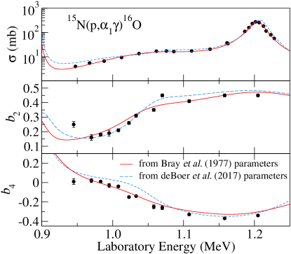
Figure 1: (Color online) The total cross section and $\gamma$-ray angular distribution coefficients for the ${}^{15}{\rm N}(p,\alpha_{1}\gamma){}^{12}{\rm C}^{*}$ reaction. The experimental results of Bray et al. (1977) are shown as points. Calculations using the Bray et al. (1977) and deBoer et al. (2017) $R$-matrix parameters are shown as the solid red and dashed blue curves, respectively.

Bray et al. (1977) also performed an $R$-matrix fit to their ${}^{15}{\rm N}(p,\alpha_{1}\gamma){}^{12}{\rm C}^{*}$ measurements and other ${}^{15}{\rm N}+p$ reaction data. They included the $b_{k}$ coefficients in their fit, but unfortunately no formulas or other descriptions of their procedures were given. They do , however, provide in Tables 2 and 3 their best fit $R$-matrix parameters, in the Lane and Thomas formalism Lane and Thomas (1958). Using these parameters in AZURE2, we have calculated $\sigma_{\rm tot}$, $b_{2}$, and $b_{4}$, with the results being very close to the calculations given by Bray et al. (1977) in Fig. 2 of their paper. Our calculations are also shown as the solid curve in our Fig. 1, where they are seen to be very close to the experimental results of Bray et al. (1977).

A comprehensive $R$-matrix analysis of the ${}^{16}{\rm O}$ compound nucleus was recently published by deBoer et al. (2017). The angular distribution coefficients $b_{2}$ and $b_{4}$ defined above were not included in the fit or otherwise considered in the analysis. However, the $R$-matrix parameters given by Ref. deBoer et al. (2017) provide an excellent description of these coefficients. In this case, the $R$-matrix parameters are given in the alternative $R$-matrix formalism Brune (2002). The $\sigma_{\rm tot}$, $b_{2}$, and $b_{4}$ resulting from using these parameters in an AZURE2 calculation are shown as the dashed curves in Fig. 1. These calculations are seen to be very close to both the Bray et al. (1977) data and the calculations using their parameters. This example demonstrates that the $R$-matrix formalism can be used to predict the $\gamma$-ray angular distributions, provided the parameters can be suitably constrained using other reaction data.

Bray et al. (1977) also presented $\gamma$-ray energy spectra measured at $\theta_{\gamma}=0$ that were also well described by their $R$-matrix fit. Again, no formulas or other descriptions of their procedures were given. Their data are shown in their Fig. 3, and unfortunately are not presented in a manner that facilitates a simple comparison with other calculations of the correlation function for $\theta_{\gamma}=0$.

VI Conclusions

The general formalism for calculating the correlation of secondary $\gamma$ rays with the beam direction and reaction products has been reviewed. The general results have been adapted to the partial-wave $T$-matrix formalism and specializations to common special cases have been presented. These specializations are well suited for calculations when the the reaction of interest is described by $R$-matrix theory. The case of the $\gamma$-ray angular distribution, with the other reaction products undetected, has been implemented in the $R$-matrix code AZURE2. This capability has been demonstrated with the example of the ${}^{15}{\rm N}(p,\alpha_{1}\gamma){}^{12}{\rm C}^{*}$ reaction. We anticipate the application of this type of analysis to several other cases. Additional measurements have already been performed at the University of Notre Dame of the ${}^{15}{\rm N}(p,\alpha_{1}\gamma){}^{12}{\rm C}^{*}$ reaction, extending the range of study to higher energies deBoer et al. .

At last two extensions to this work can be envisioned. One additional possibility is the situation where the initial reaction is a radiative capture reaction. Another is the case of $\gamma$-ray cascades following a reaction. This scenario can be addressed using the formalism given by Rose and Brink (1967).

References

• Lane and Thomas (1958) A. M. Lane and R. G. Thomas, “R-matrix theory of nuclear reactions,” Rev. Mod. Phys. 30, 257–353 (1958).
• Descouvemont and Baye (2010) P. Descouvemont and D. Baye, “The R-matrix theory,” Reports on Progress in Physics 73, 036301 (2010).
• Azuma et al. (2010) R. E. Azuma, E. Uberseder, E. C. Simpson, C. R. Brune, H. Costantini, R. J. de Boer, J. Görres, M. Heil, P. J. LeBlanc, C. Ugalde,  and M. Wiescher, “azure: An R-matrix code for nuclear astrophysics,” Phys. Rev. C 81, 045805 (2010).
• Nelson and Wender (1994) R. O. Nelson and S. A. Wender, “Neutron-induced gamma-ray production from carbon and nitrogen,” Los Alamos Report No. LA-UR-94-1767  (1994).
• Nelson et al. (2001) R. O. Nelson, M. B. Chadwick, A. Michaudon,  and P. G. Young, “High-resolution measurements and calculations of photon-production cross sections for ${{}^{16}{\rm O}(n,x\gamma)}$ reactions induced by neutrons with energies between 4 and 200 MeV,” Nuclear Science and Engineering 138, 105–144 (2001).
• Bray et al. (1977) K. H. Bray, A. D. Frawley, T. R. Ophel,  and F. C. Barker, “Levels of ${{}^{16}{\rm O}}$ near 13 MeV excitation from ${{}^{15}{\rm N}+{\rm p}}$ reactions,” Nuclear Physics A 288, 334–350 (1977).
• Cloud and Ophel (1969) S. D. Cloud and T. R. Ophel, “The 1080 keV resonance of the ${{}^{15}{\rm N}(p,\alpha\gamma)}$ reaction,” Nuclear Physics A 136, 592–598 (1969).
• Stark et al. (1970) W. J. Stark, P. M. Cockburn,  and R. W. Krone, “Spin assignments of states in ${{\mathrm{Mg}}^{24}}$ from an analysis of Doppler-broadened gamma rays,” Phys. Rev. C 1, 1752–1756 (1970).
• Tryti et al. (1973) S. Tryti, T. Holtebekk,  and J. Rekstad, “Angular distributions of protons near resonance for the reaction ${{}^{12}{\rm C}(d,p\gamma){}^{13}{\rm C}}$ obtained by shape studies of $\gamma$-ray lines,” Nuclear Physics A 201, 135–144 (1973).
• Tryti et al. (1975) S. Tryti, T. Holtebekk,  and F. Ugletveit, “Angular distributions of protons from the reaction ${{}^{12}{\rm C}(d,p\gamma){}^{13}{\rm C}}$ obtained by shape studies of $\gamma$-ray lines,” Nuclear Physics A 251, 206–224 (1975).
• Kiptily et al. (1999) V. G. Kiptily, D. N. Doinikov, V. O. Naidenov, I. A. Polunovsky, I. N. Chugunov, A. E. Shevelev, S. N. Abramovich, V. A. Agureev,  and S. V. Trusillo, “Doppler contour of $\gamma$ lines and angular distribution of $\gamma$ quanta and protons in the ${{}^{10}{\rm B}(\alpha,p\gamma){}^{13}{\rm C}}$ reaction,” Bulletin of the Russian Academ of Sciences: Physics 63, 716–723 (1999).
• Satchler (1954) G. R. Satchler, “The angular correlation of three nuclear radiations,” Phys. Rev. 94, 1304–1306 (1954).
• Devons and Goldfarb (1957) S. Devons and L. J. B. Goldfarb, “Angular correlations,” in Kernreaktionen III / Nuclear Reactions III (Springer, Berlin, 1957) pp. 362–554.
• Wolfenstein (1956) L. Wolfenstein, “Polarization of fast nucleons,” Annual Review of Nuclear Science 6, 43–76 (1956).
• Welton (1963) T. A. Welton, “The theory of polarization in reactions and scattering,” in Fast Neutron Physics, Part II: Experiments and Theory, edited by J. B. Marion and J. L. Fowler (Interscience, New York, 1963) pp. 1317–1377.
• Heiss (1972) P. Heiss, “On the theory of polarization in nuclear reactions and scattering,” Zeitschrift für Physik A 251, 159–167 (1972).
• Simonius (1974) M. Simonius, “Theory of polarization measurements: Observables, amplitudes and symmetries,” in Polarization Nuclear Physics, edited by D. Fick (Springer, Berlin, 1974) pp. 38–87.
• Schieck (2012) Hans Paetz gen. Schieck, Nuclear Physics with Polarized Particles (Springer, Berlin, 2012).
• Sheldon (1963) Eric Sheldon, “Angular correlation in inelastic nucleon scattering,” Rev. Mod. Phys. 35, 795–852 (1963).
• Rybicki et al. (1970) F. Rybicki, T. Tamura,  and G. R. Satchler, “Particle-gamma angular correlations following nuclear reactions,” Nuclear Physics A 146, 659–676 (1970).
• Rose and Brink (1967) H. J. Rose and D. M. Brink, “Angular distributions of gamma rays in terms of phase-defined reduced matrix elements,” Rev. Mod. Phys. 39, 306–347 (1967).
• Satchler (1983) G. R. Satchler, Direct Nuclear Reactions (Clarendon, Oxford, 1983).
• Thompson (1988) Ian J. Thompson, “Coupled reaction channels calculations in nuclear physics,” Computer Physics Reports 7, 167–212 (1988).
• deBoer et al. (2017) R. J. deBoer, J. Görres, M. Wiescher, R. E. Azuma, A. Best, C. R. Brune, C. E. Fields, S. Jones, M. Pignatari, D. Sayre, K. Smith, F. X. Timmes,  and E. Uberseder, “The ${{}^{12}{\rm C}(\alpha,\gamma)^{16}{\rm O}}$ reaction and its implications for stellar helium burning,” Rev. Mod. Phys. 89, 035007 (2017).
• Brune (2002) C. R. Brune, “Alternative parametrization of R-matrix theory,” Phys. Rev. C 66, 044611 (2002).
• (26) R. J. deBoer, C. R. Brune, A. Boeltzig, K. T. Macon, S. Aguilar, S. P. Burcher, O. Gomez, B. Frentz, G. Gilardy, S. Henderson, G. Imbriani, K.L. Jones, R. Kelmar, J. M. Kovoor, S. Mosby, M. Renaud, K. Smith, B. Vande Kolk,  and M. Wiescher, “Investigation of secondary gamma-ray angular distributions using the ${{}^{15}{\rm N}(p,\alpha_{1}\gamma){}^{12}{\rm C}}$ reaction,” Phys. Rev. C (submitted) .