Electromagnetic surface waves at exceptional points

Abstract

Guided by the planar interface of two dissimilar linear, homogeneous mediums, a Voigt surface wave arises due to an exceptional point of either of the two matrixes necessary to describe the spatial characteristics in the direction normal to the planar interface. There is no requirement for either or both partnering mediums to be dissipative, unlike a Voigt plane wave which can propagate only in a dissipative medium.

1 Introduction

Exceptional points [1] have gained considerable currency this century in the literature on electromagnetics wave propagation in a passive linear homogeneous medium. The planewave solution of the time-harmonic Maxwell postulates in this medium is given by

$${\bf{E}}({\bf{r}},\omega)={\bf{U}}_{1}\exp\left(ik_{1}\hat{{\bf{a}}}\mbox{ \tiny{${}^{\bullet}$} }{\bf{r}}\right)+{\bf{U}}_{2}\exp\left(ik_{2}\hat{{\bf{a}}}\mbox{ \tiny{${}^{\bullet}$} }{\bf{r}}\right)\,,$$ (1)

where ${\bf{E}}\in\mathbb{C}^{3}$ is the electric field phasor, ${\bf{r}}\in\mathbb{R}^{3}$ is the position vector, ${\bf{U}}_{1}\in\mathbb{C}^{3}$ and ${\bf{U}}_{2}\in\mathbb{C}^{3}$ are amplitude vectors, $i=\sqrt{-1}$, $k_{1}\in\mathbb{C}$ and $k_{2}\in\mathbb{C}$ are wavenumbers with non-negative imaginary parts, the unit vector $\hat{{\bf{a}}}\in\mathbb{R}^{3}$ delineates the direction of propagation, and an $\exp(-i\omega t)$ dependence on time $t$ is implicit with $\omega$ as the angular frequency.

However, Eq. (1) is not always applicable. Circumstances may arise when $k_{2}=k_{1}$ and ${\bf{U}}_{1}\parallel{\bf{U}}_{2}$ [2, 3], as was experimentally shown by Voigt [4] in 1902 with biaxial absorbing dielectric mediums. There may be four isolated values of $\hat{{\bf{a}}}$ for which Eq. (1) has to be replaced by [5, 6]

$${\bf{E}}({\bf{r}})=\left[{\bf{V}}_{1}+i(\hat{{\bf{a}}}\mbox{ \tiny{${}^{\bullet}$} }{\bf{r}}){\bf{V}}_{2}\right]\exp\left(ik_{1}\hat{{\bf{a}}}\mbox{ \tiny{${}^{\bullet}$} }{\bf{r}}\right)\,,$$ (2)

where ${\bf{V}}_{1}\in\mathbb{C}^{3}$ and ${\bf{V}}_{2}\in\mathbb{C}^{3}$. The linear dependence on the distance $\hat{{\bf{a}}}\mbox{ \tiny{${}^{\bullet}$} }{\bf{r}}$ along the direction of propagation in Eq. (2), in addition to the usual exponential dependence common to both Eqs. (1) and (2), is the hallmark of the Voigt plane wave [7, 8, 9]. Voigt plane waves cannot propagate in isotropic and uniaxial dielectric mediums, whether dissipative or not; neither can Voigt plane waves propagate in nondissipative biaxial dielectric mediums.

The specific directions of propagation of a Voigt plane wave in a particular medium are called the singular axes [4] of that medium. These axes appear in band diagrams as exceptional points [8, 10]. Exceptional points are readily appreciated through matrix algebra. Let the unit vector $\hat{{\bf{b}}}\in\mathbb{R}^{3}$ be orthogonal to $\hat{{\bf{a}}}$. Then, the unit vector $\hat{{\bf{c}}}=\hat{{\bf{a}}}\times\hat{{\bf{b}}}$ is orthogonal to both $\hat{{\bf{a}}}$ and $\hat{{\bf{b}}}$ and the triad $\left\{\hat{{\bf{a}}},\hat{{\bf{b}}},\hat{{\bf{c}}}\right\}$ forms a right-handed Cartesian coordinate system. The Maxwell divergence postulates then yield $\hat{{\bf{a}}}\mbox{ \tiny{${}^{\bullet}$} }{\bf{B}}({\bf{r}},\omega)\equiv 0$ and $\hat{{\bf{a}}}\mbox{ \tiny{${}^{\bullet}$} }{\bf{D}}({\bf{r}},\omega)\equiv 0$, where ${\bf{B}}({\bf{r}},\omega)\in\mathbb{C}^{3}$ is the magnetic flux density phasor and ${\bf{D}}({\bf{r}},\omega)\in\mathbb{C}^{3}$ is the electric displacement phasor. Planewave propagation can then be investigated by forming the matrix ordinary differential equation

$$\frac{d}{d(\hat{{\bf{a}}}\mbox{ \tiny{${}^{\bullet}$} }{\bf{r}})}\left[\begin{matrix}\hat{{\bf{b}}}\mbox{ \tiny{${}^{\bullet}$} }{\bf{D}}\\ \hat{{\bf{c}}}\mbox{ \tiny{${}^{\bullet}$} }{\bf{D}}\\ \hat{{\bf{b}}}\mbox{ \tiny{${}^{\bullet}$} }{\bf{B}}\\ \hat{{\bf{c}}}\mbox{ \tiny{${}^{\bullet}$} }{\bf{B}}\end{matrix}\right]=\left[\underline{\underline{W}}\right]\mbox{ \tiny{${}^{\bullet}$} }\left[\begin{matrix}\hat{{\bf{b}}}\mbox{ \tiny{${}^{\bullet}$} }{\bf{D}}\\ \hat{{\bf{c}}}\mbox{ \tiny{${}^{\bullet}$} }{\bf{D}}\\ \hat{{\bf{b}}}\mbox{ \tiny{${}^{\bullet}$} }{\bf{B}}\\ \hat{{\bf{c}}}\mbox{ \tiny{${}^{\bullet}$} }{\bf{B}}\end{matrix}\right]\,,$$ (3)

where the 4$\times$4 matrix $\left[\underline{\underline{W}}\right]$ is independent of ${\bf{r}}$. Ordinarily but not always, $\left[\underline{\underline{W}}\right]$ will have four eigenvalues, each of algebraic multiplicity $1$ and geometric multiplicity $1$. The occurrence of an exceptional point is unambiguously indicated by an eigenvalue of algebraic multiplicity $2$ and geometric multiplicity $1$.

Whereas previous research on exceptional points in electromagnetics has been largely confined to planewave propagation in dissipative mediums, exceptional points are also relevant to surface-wave propagation, as we have illustrated in the following sections of this Letter. The propagation of an electromagnetic surface wave is guided by the planar interface of two mediums ${\cal A}$ and ${\cal B}$ whose constitutive parameters are invariant in any direction wholly contained in the interface plane [11, 12]. Exceptional points can show up when at least one of the two mediums is homogeneous. Salient features of the underlying theory of Voigt surface waves are presented in Sec. 2, with both mediums passive, linear, homogeneous, and bianisotropic [13]. Three examples are provided in Sec. 3.

The following notation is adopted: The permittivity and permeability of free space are denoted by $\varepsilon_{\scriptscriptstyle 0}$ and $\mu_{\scriptscriptstyle 0}$, respectively. The free-space wavenumber is written as $k_{\scriptscriptstyle 0}=\omega\sqrt{\varepsilon_{\scriptscriptstyle 0}\mu_{\scriptscriptstyle 0}}$. Vectors are in boldface, $\left\{\hat{{\bf{u}}}_{1},\hat{{\bf{u}}}_{2},\hat{{\bf{u}}}_{3}\right\}$ is the triad of unit vectors aligned with the Cartesian axes, and the position vector ${\bf{r}}=x_{1}\hat{{\bf{u}}}_{1}+x_{2}\hat{{\bf{u}}}_{2}+x_{3}\hat{{\bf{u}}}_{3}$. Dyadics are double underlined [14]. Square brackets enclose matrixes and column vectors. The superscript ^T denotes the transpose. The real and imaginary parts of complex quantities are delivered by the operators $\mbox{Re}\left\{\cdot\right\}$ and $\mbox{Im}\left\{\cdot\right\}$, respectively.

2 Theory

In the canonical boundary-value problem for surface-wave propagation [12], medium ${\cal A}$ occupies the half-space $x_{3}>0$ and medium ${\cal B}$ the half-space $x_{3}<0$, their interface being the plane $x_{3}=0$.

Medium ${\cal A}$ is taken to have the constitutive relations

$$\left.\begin{array}[]{l}{\bf{D}}({\bf{r}},\omega)=\varepsilon_{\scriptscriptstyle 0}\underline{\underline{\varepsilon}}_{\cal A}(\omega)\mbox{ \tiny{${}^{\bullet}$} }{\bf{E}}({\bf{r}},\omega)+\underline{\underline{\xi}}_{\cal A}(\omega)\mbox{ \tiny{${}^{\bullet}$} }{\bf{H}}({\bf{r}},\omega)\\[5.0pt] {\bf{B}}({\bf{r}},\omega)=\underline{\underline{\zeta}}_{\cal A}(\omega)\mbox{ \tiny{${}^{\bullet}$} }{\bf{E}}({\bf{r}},\omega)+\mu_{\scriptscriptstyle 0}\underline{\underline{\mu}}_{\cal A}(\omega)\mbox{ \tiny{${}^{\bullet}$} }{\bf{H}}({\bf{r}},\omega)\end{array}\right\}\,,\quad x_{3}>0\,,$$ (4)

where $\underline{\underline{\varepsilon}}_{\cal A}$ is the relative permittivity dyadic, $\underline{\underline{\mu}}_{\cal A}$ is the relative permeability dyadic, and $\underline{\underline{\xi}}_{\cal A}$ as well as $\underline{\underline{\zeta}}_{\cal A}$ are the magnetoelectric dyadics. Medium ${\cal B}$ has the analogous constitutive relations

$$\left.\begin{array}[]{l}{\bf{D}}({\bf{r}},\omega)=\varepsilon_{\scriptscriptstyle 0}\underline{\underline{\varepsilon}}_{\cal B}(\omega)\mbox{ \tiny{${}^{\bullet}$} }{\bf{E}}({\bf{r}},\omega)+\underline{\underline{\xi}}_{\cal B}(\omega)\mbox{ \tiny{${}^{\bullet}$} }{\bf{H}}({\bf{r}},\omega)\\[5.0pt] {\bf{B}}({\bf{r}},\omega)=\underline{\underline{\zeta}}_{\cal B}(\omega)\mbox{ \tiny{${}^{\bullet}$} }{\bf{E}}({\bf{r}},\omega)+\mu_{\scriptscriptstyle 0}\underline{\underline{\mu}}_{\cal B}(\omega)\mbox{ \tiny{${}^{\bullet}$} }{\bf{H}}({\bf{r}},\omega)\end{array}\right\}\,,\quad x_{3}<0\,.$$ (5)

Henceforth, the dependences of various quantities on $\omega$ are not explicitly identified.

The electromagnetic field phasors for surface-wave propagation are expressed everywhere as [12]

$$\left.\begin{array}[]{l}{\bf{E}}({\bf{r}})=\left[e_{1}(x_{3})\hat{{\bf{u}}}_{1}+e_{2}(x_{3})\hat{{\bf{u}}}_{2}+e_{3}(x_{3})\hat{{\bf{u}}}_{3}\right]\,\exp\left[iq\left(x_{1}\cos\psi+x_{2}\sin\psi\right)\right]\\[4.0pt] {\bf{H}}({\bf{r}})=\left[h_{1}(x_{3})\hat{{\bf{u}}}_{1}+h_{2}(x_{3})\hat{{\bf{u}}}_{2}+h_{3}(x_{3})\hat{{\bf{u}}}_{3}\right]\,\exp\left[iq\left(x_{1}\cos\psi+x_{2}\sin\psi\right)\right]\end{array}\right\}\,,\qquad x_{3}\in(-\infty,\infty)\,,$$ (6)

where ${q}\in\mathbb{C}$ is the surface wavenumber. The angle $\psi\in\left[0,2\pi\right)$ specifies the direction of propagation in the $x_{1}$-$x_{2}$ plane, relative to the $x_{1}$ axis. The phasor representations (6), when combined with the source-free Faraday and Ampére–Maxwell equations, deliver the 4$\times$4 matrix ordinary differential equations [15, 16]

$$\frac{d}{dx_{3}}\left[{\bf{f}}(x_{3})\right]=\left\{\begin{array}[]{ll}i[\underline{\underline{P}}_{\cal A}]\mbox{ \tiny{${}^{\bullet}$} }\left[{\bf{f}}(x_{3})\right]\,,&x_{3}>0\,,\vspace{8pt}\\ i[\underline{\underline{P}}_{\cal B}]\mbox{ \tiny{${}^{\bullet}$} }\left[{\bf{f}}(x_{3})\right]\,,&x_{3}<0\,,\end{array}\right.$$ (7)

wherein the column 4-vector

$$\left[{\bf{f}}(x_{3})\right]=\left[\begin{array}[]{c}e_{1}(x_{3}),\quad e_{2}(x_{3}),\quad h_{1}(x_{3}),\quad h_{2}(x_{3})\end{array}\right]^{T}$$ (8)

depends on $x_{3}$, but the 4$\times$4 matrixes $[\underline{\underline{P}}_{\cal A}]$ and $[\underline{\underline{P}}_{\cal B}]$ are independent of $x_{3}$. Explicit expressions for $[\underline{\underline{P}}_{\cal A}]$ and $[\underline{\underline{P}}_{\cal B}]$ are available elsewhere [12, Sec. 3.3.1], but are too cumbersome for repetition here. The $x_{1}$-directed and $x_{2}$-directed components of the phasors are algebraically connected to their $x_{3}$-directed components [13].

2.1 Half-space $x_{3}>0$

2.1.1 Ordinary surface waves

Let us first consider the ordinary surface waves for which $[\underline{\underline{P}}_{\cal A}]$ has four eigenvalues, each with algebraic multiplicity $1$ and geometric multiplicity $1$. Eigenvalues with negative imaginary parts are irrelevant for surface-wave propagation. Denoted by $\alpha_{{\cal A}1}$ and $\alpha_{{\cal A}2}$, the two eigenvalues appropriate for surface-wave analysis are such that $\mbox{Im}\left\{\alpha_{{\cal A}1}\right\}>0$ and $\mbox{Im}\left\{\alpha_{{\cal A}2}\right\}>0$. Explicit expressions for the corresponding eigenvectors $\left[{\bf{v}}_{{\cal A}1}\right]$ and $\left[{\bf{v}}_{{\cal A}2}\right]$ can be derived by solving the equations

$$\left([\underline{\underline{P}}_{\cal A}]-\alpha_{{\cal A}n}\left[\underline{\underline{I}}\right]\right)\mbox{ \tiny{${}^{\bullet}$} }\left[{\bf{v}}_{{\cal A}n}\right]=\left[{\bf{0}}\right]\,,\qquad n\in\left\{1,2\right\}\,,$$ (9)

where $\left[\underline{\underline{I}}\right]$ is the 4$\times$4 identity matrix and $\left[{\bf{0}}\right]$ is the null column 4-vector. The two remaining eigenvalues, $\alpha_{{\cal A}3}$ and $\alpha_{{\cal A}4}$, of $[\underline{\underline{P}}_{\cal A}]$ are irrelevant because $\mbox{Im}\left\{\alpha_{{\cal A}3}\right\}<0$ and $\mbox{Im}\left\{\alpha_{{\cal A}4}\right\}<0$.

Thus the general solution of Eq. (7)₁ applicable to ordinary surface waves that decay as $x_{3}\to+\infty$ is given as

$$\left[{\bf{f}}(x_{3})\right]=C_{{\cal A}1}\left[{\bf{v}}_{{\cal A}1}\right]\exp\left(i\alpha_{{\cal A}1}x_{3}\right)+C_{{\cal A}2}\left[{\bf{v}}_{{\cal A}2}\right]\exp\left(i\alpha_{{\cal A}2}x_{3}\right)\,,\quad x_{3}>0\,.$$ (10)

The complex-valued constants $C_{{\cal A}1}$ and $C_{{\cal A}2}$ herein are fixed by applying boundary conditions at $x_{3}=0$. These boundary conditions involve

$$\left[{\bf{f}}(0^{+})\right]=C_{{\cal A}1}\left[{\bf{v}}_{{\cal A}1}\right]+C_{{\cal A}2}\left[{\bf{v}}_{{\cal A}2}\right]\,.$$ (11)

2.1.2 Surface wave at an exceptional point

Both eigenvalues with positive imaginary parts must be equal at an exceptional point, i.e., $\alpha_{{\cal A}1}=\alpha_{{\cal A}2}=\alpha_{\cal A}$, and the value of $q$ can be ascertained thereby. The corresponding eigenvector $\left[{\bf{v}}_{\cal A}\right]$ has to be determined first by solving

$$\left(\left[\underline{\underline{P}}_{\cal A}\right]-\alpha_{{\cal A}}\left[\underline{\underline{I}}\right]\right)\mbox{ \tiny{${}^{\bullet}$} }\left[{\bf{v}}_{{\cal A}}\right]=\left[{\bf{0}}\right]\,,$$ (12)

and a corresponding generalized eigenvector $\left[{\bf{w}}_{\cal A}\right]$ has to be then determined by solving [5]

$$\left(\left[\underline{\underline{P}}_{\cal A}\right]-\alpha_{{\cal A}}\left[\underline{\underline{I}}\right]\right)\mbox{ \tiny{${}^{\bullet}$} }\left[{\bf{w}}_{{\cal A}}\right]=\left[{\bf{v}}_{{\cal A}}\right]\,.$$ (13)

Thus, the general solution of Eq. (7)₁ representing a surface wave that decays as $x_{3}\to+\infty$ and holds at an exceptional point can be stated as

$$\left[{\bf{f}}(x_{3})\right]=\Big{(}C_{{\cal A}1}\left[{\bf{v}}_{{\cal A}}\right]+C_{{\cal A}2}\left\{ix_{3}\,\left[{\bf{v}}_{{\cal A}}\right]+\left[{\bf{w}}_{{\cal A}}\right]\right\}\Big{)}\exp\left(i\alpha_{{\cal A}}x_{3}\right)\,,\quad x_{3}>0\,.$$ (14)

The complex-valued constants $C_{{\cal A}1}$ and $C_{{\cal A}2}$ herein are fixed by applying boundary conditions at $x_{3}=0$. These boundary conditions involve

$$\left[{\bf{f}}(0^{+})\right]=C_{{\cal A}1}\left[{\bf{v}}_{{\cal A}}\right]+C_{{\cal A}2}\left[{\bf{w}}_{{\cal A}}\right]\,.$$ (15)

2.2 Half-space $x_{3}<0$

Equation (7)₂ has to be solved in the same way as Eq. (7)₁. The matrix $[\underline{\underline{P}}_{\cal B}]$ has $\alpha_{{\cal B}n}$ and $[{\bf{v}}_{{\cal B}n}]$, $n\in\left[1,4\right]$, as its $n$th eigenvalue and eigenvector, respectively. Without loss of generality, we assume that each of the four eigenvalues of $[\underline{\underline{P}}_{\cal B}]$ has algebraic multiplicity $1$ and geometric multiplicity $1$. After labeling the eigenvalues such that $\mbox{Im}\left\{{\alpha_{{\cal B}3}}\right\}<0$ and $\mbox{Im}\left\{{\alpha_{{\cal B}4}}\right\}<0$, we set

$$[{\bf{f}}(0^{-})]=C_{{\cal B}3}\left[{\bf{v}}_{{\cal B}3}\right]+C_{{\cal B}4}\left[{\bf{v}}_{{\cal B}4}\right]$$ (16)

for surface-wave propagation, where the complex-valued constants $C_{{\cal B}3}$ and $C_{{\cal B}4}$ are fixed by applying boundary conditions at $x_{3}=0$. The other two eigenvalues of $[\underline{\underline{P}}_{\cal B}]$ pertain to waves that amplify as $x_{3}\to-\infty$ and cannot therefore contribute to the surface wave.

2.3 Dispersion equation

The continuity of the tangential components of the electric and magnetic field phasors across the interface plane $x_{3}=0$ imposes four boundary conditions that are represented compactly as

$$\left[{\bf{f}}(0^{+})\right]=\left[{\bf{f}}(0^{-})\right]\,.$$ (17)

Accordingly,

$$\left[\underline{\underline{Y}}\right]\mbox{ \tiny{${}^{\bullet}$} }\left[\>C_{{\cal A}1},\quad C_{{\cal A}2},\quad C_{{\cal B}3},\quad C_{{\cal B}4}\>\right]^{T}=\left[{\bf{0}}\right]\,,$$ (18)

wherein the 4$\times$4 characteristic matrix $\left[\underline{\underline{Y}}\right]$ must be singular for surface-wave propagation [12]. The dispersion equation

$$\left|\left[\underline{\underline{Y}}\right]\right|=0,$$ (19)

can be numerically solved for $q$ for a fixed value of $\psi$, by the Newton–Raphson method [17] for example.

3 Illustrative Examples

Examples of electromagnetic surface waves corresponding to the exceptional points of $[\underline{\underline{P}}_{\cal A}]$ have recently become available [18, 19, 20], though the exceptional nature of those surface waves has not been demonstrated yet. In order to highlight the exceptional nature of the occurrence of a Voigt surface wave, we now present three examples. For all these examples, we have set $\underline{\underline{\xi}}_{{\cal A}}=\underline{\underline{\xi}}_{{\cal B}}=\underline{\underline{0}}$, $\underline{\underline{\zeta}}_{{\cal A}}=\underline{\underline{\zeta}}_{{\cal B}}=\underline{\underline{0}}$, and $\underline{\underline{\mu}}_{{\cal A}}=\underline{\underline{\mu}}_{{\cal B}}=\underline{\underline{I}}$, where $\underline{\underline{0}}$ is the null dyadic and $\underline{\underline{I}}=\hat{{\bf{u}}}_{1}\hat{{\bf{u}}}_{1}+\hat{{\bf{u}}}_{2}\hat{{\bf{u}}}_{2}+\hat{{\bf{u}}}_{3}\hat{{\bf{u}}}_{3}$ is the identity dyadic.

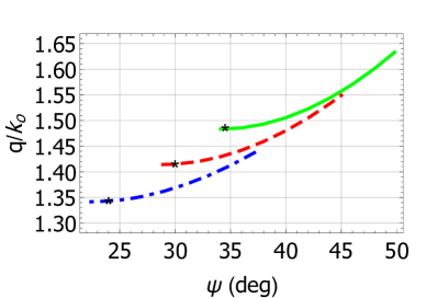
(a)

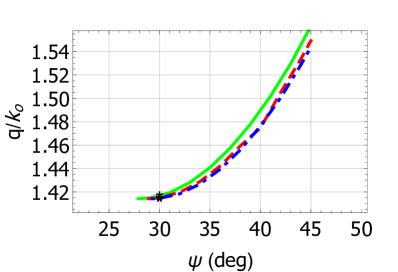
(b)

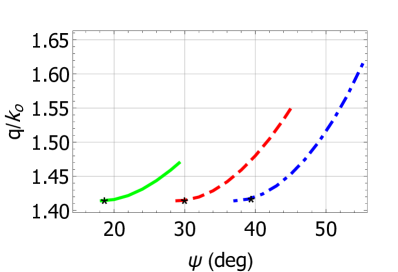
(c)

Figure 1: Plots of $q/k_{\scriptscriptstyle 0}$ versus $\psi$ for Dyakonov surface waves guided by the planar interface of a non-dissipative uniaxial dielectric medium and a non-dissipative isotropic dielectric medium described by Eqs. (20). (a) $\varepsilon^{s}_{\cal A}=1.5,\varepsilon^{t}_{\cal A}=6$, and $\varepsilon_{\cal B}=1.8$ (blue broken-dashed curve), $2$ (red dashed curve), $2.2$ (green solid curve); (b) $\varepsilon^{s}_{\cal A}=1.5,\varepsilon_{\cal B}=2$, and $\varepsilon^{t}_{\cal B}=5.5$ (blue broken-dashed curve), $6$ (red dashed curve), $6.5$ (green solid curve); and (c) $\varepsilon^{t}_{\cal A}=6,\varepsilon_{\cal B}=2$, and $\varepsilon^{s}_{\cal A}=1.2$ (blue broken-dashed curve), $1.5$ (red dashed curve), $1.8$ (green solid curve). A Dyakonov–Voigt surface wave corresponding to an exceptional point of $\left[{\underline{\underline{P}}}_{\cal A}\right]$ is identified by a black star in each curve.

We chose the relative permittivity dyadic of medium ${\cal A}$ to be uniaxial with its preferred axis parallel to $\hat{{\bf{u}}}_{1}$, and the relative permittivity dyadic of medium ${\cal B}$ to represent a scalar medium [18] for all three examples; hence,

$$\left.\begin{array}[]{l}\underline{\underline{\varepsilon}}_{\mathcal{A}}=\varepsilon_{\mathcal{A}}^{\rm s}\underline{\underline{I}}+\left(\varepsilon_{\mathcal{A}}^{\rm t}-\varepsilon_{\mathcal{A}}^{\rm s}\right)\,\hat{{\bf{u}}}_{1}\hat{{\bf{u}}}_{1}\\[6.0pt] \underline{\underline{\varepsilon}}_{\mathcal{B}}=\varepsilon_{\mathcal{B}}\underline{\underline{I}}\end{array}\right\}\,.$$ (20)

For these constitutive relations, if a surface wave exists for angle $\psi=\psi^{\star}$, then surface-wave propagation is also possible for $\psi=-\psi^{\star}$ and $\psi=\pi\pm\psi^{\star}$.

3.1 Example No. 1

For the first example, we chose $\varepsilon_{\mathcal{A}}^{\rm s}\in\mathbb{R}$, $\varepsilon_{\mathcal{A}}^{\rm t}\in\mathbb{R}$, and $\varepsilon_{\mathcal{B}}\in\mathbb{R}$. Furthermore, we chose all three constitutive parameters to be positive. Ordinary surface waves guided by the planar interface of the chosen mediums are classified as Dyakonov surface waves [21, 22, 23].

Figure 1 presents plots of the normalized wavenumber $q/k_{\scriptscriptstyle 0}$ versus $\psi$ found for the quadrant $0\leq\psi\leq\pi/2$ when all three constitutive parameters $\varepsilon_{\mathcal{A}}^{\rm s}$, $\varepsilon_{\mathcal{A}}^{\rm t}$, and $\varepsilon_{\mathcal{B}}$ are real and positive. Despite both partnering mediums ${\cal A}$ and ${\cal B}$ being non-dissipative, a solitary point on each curve in Fig. 1 is the manifestation of an exceptional point of $[\underline{\underline{P}}_{\cal A}]$. The surface wave corresponding to this exceptional point is classified as a Dyakonov–Voigt surface wave [18].

The values of $\varepsilon_{\mathcal{B}}$, $\varepsilon_{\mathcal{A}}^{\rm t}$, and $\varepsilon_{\mathcal{A}}^{\rm s}$ were varied for Figs. 1(a), (b), and (c), respectively. While the angle of propagation $\psi$ for the Dyakonov–Voigt surface wave is highly sensitive to the values of $\varepsilon_{\mathcal{A}}^{\rm s}$ and $\varepsilon_{\mathcal{B}}$ as we see in Figs. 1(a) and (c), the same is not true of $\varepsilon_{\mathcal{A}}^{\rm t}$ as can be observed in Fig. 1(b). Also, while the surface wavenumber $q$ for the Dyakonov–Voigt surface wave is highly sensitive to the values of $\varepsilon_{\mathcal{B}}$ as we see in Fig. 1(a), the same is not true of $\varepsilon_{\mathcal{A}}^{\rm s}$ and $\varepsilon_{\mathcal{A}}^{\rm t}$ as we note from Figs. 1(b) and (c).

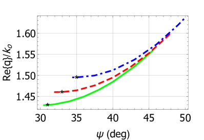
(a)

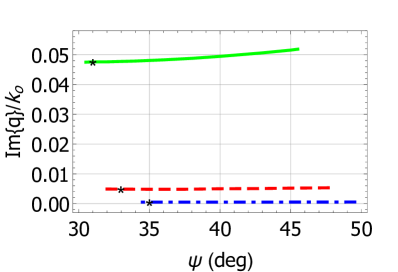
(b)

Figure 2: Plots of (a) ${\rm Re}\left\{{q}\right\}/k_{\scriptscriptstyle 0}$ and (b) ${\rm Im}\left\{{q}\right\}/k_{\scriptscriptstyle 0}$ versus $\psi$ for Dyakonov surface waves guided by the planar interface of a dissipative uniaxial dielectric medium and a dissipative isotropic dielectric medium described by Eqs. (20). $\varepsilon^{s}_{\cal A}=1.5+\delta i$ and $\varepsilon^{t}_{\cal A}=6+4\delta i$ with $\delta=0.1$, $\varepsilon_{\cal B}=2.0398+0.1360i$ (green solid curves); $\delta=0.01$, $\varepsilon_{\cal B}=2.1320+0.0142i$ (red dashed curves); and $\delta=0.001$, $\varepsilon_{\cal B}=2.2354+0.0015i$ (blue broken-dashed curves). On each curve, a Dyakonov–Voigt surface wave corresponding to an exceptional point of $\left[{\underline{\underline{P}}}_{\cal A}\right]$ is identified by a black star.

3.2 Example No. 2

Whereas both partnering mediums were chosen to be non-dissipative for Fig. 1, both were chosen to be dissipative for the second example, i.e., $\varepsilon_{\mathcal{A}}^{\rm s}\in\mathbb{C}$, $\varepsilon_{\mathcal{A}}^{\rm t}\in\mathbb{C}$, and $\varepsilon_{\mathcal{B}}\in\mathbb{C}$. Also, both the real and the imaginary parts of every one of these three constitutive parameters were chosen to be positive.

Plots of ${\rm Re}\left\{{q}\right\}/k_{\scriptscriptstyle 0}$ and ${\rm Im}\left\{{q}\right\}/k_{\scriptscriptstyle 0}$ versus $\psi$ found for the quadrant $0\leq\psi\leq\pi/2$ are shown in Fig. 2. Each curve in this figure has a solitary solution that is identified by a black star. Every star represents a Dyakonov–Voigt surface wave engendered by an exceptional point of $[\underline{\underline{P}}_{\cal A}]$ [19].

The degrees of dissipation of the partnering materials, as well as $\mbox{Re}\left\{\varepsilon_{\cal B}\right\}$, were varied for Fig. 2. The angle of propagation $\psi$ and the real and imaginary parts of the surface wavenumber $q$ for the Dyakonov–Voigt surface waves represented in Fig. 2 are highly sensitive to the degrees of dissipation of the partnering materials and $\mbox{Re}\left\{\varepsilon_{\cal B}\right\}$.

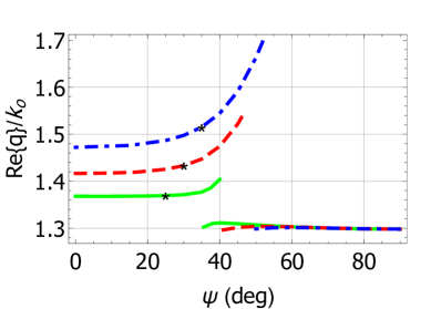
(a)

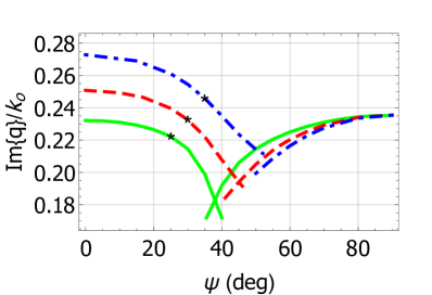
(b)

Figure 3: Plots of ${\rm Re}\left\{{q}\right\}/k_{\scriptscriptstyle 0}$ and ${\rm Im}\left\{{q}\right\}/k_{\scriptscriptstyle 0}$ versus $\psi$ for surface-plasmon-polariton waves guided by the planar interface of a dissipative uniaxial dielectric medium and an isotropic plasmonic medium described by Eqs. (20). $\varepsilon_{\cal B}=-16.07+0.44i$ and $\varepsilon^{s}_{\cal A}=1.5+0.5i$ with $\varepsilon^{t}_{\cal A}=3.1559+0.0459i$ (green solid curves), $4.4516+0.2285i$ (red dashed curves), $5.9760+0.4572i$ (blue broken-dashed curves). A surface-plasmon-polariton wave corresponding to an exceptional point of $\left[{\underline{\underline{P}}}_{\cal A}\right]$ is identified by a black star.

3.3 Example No. 3

For the third and final example, we again chose $\varepsilon_{\mathcal{A}}^{\rm s}\in\mathbb{C}$, $\varepsilon_{\mathcal{A}}^{\rm t}\in\mathbb{C}$, and $\varepsilon_{\mathcal{B}}\in\mathbb{C}$. With ${\rm Re}\left\{\varepsilon^{s}_{\cal A}\right\}>0$, ${\rm Im}\left\{\varepsilon^{s}_{\cal A}\right\}>0$, ${\rm Re}\left\{\varepsilon^{t}_{\cal A}\right\}>0$, and ${\rm Im}\left\{\varepsilon^{t}_{\cal A}\right\}>0$, medium ${\cal A}$ is dissipative dielectric; however, with ${\rm Re}\left\{\varepsilon_{\cal B}\right\}<0$ and ${\rm Im}\left\{\varepsilon_{\cal B}\right\}>0$, medium ${\cal B}$ is plasmonic. Ordinary surface waves guided by the planar interface of these two mediums are called surface-plasmon-polariton waves [24, 25].

Plots of ${\rm Re}\left\{{q}\right\}/k_{\scriptscriptstyle 0}$ and ${\rm Im}\left\{{q}\right\}/k_{\scriptscriptstyle 0}$ versus $\psi$ found for the quadrant $0\leq\psi\leq\pi/2$ are shown in Fig. 3. Surface-plasmon-polariton waves exist for all $\psi\in\left[0,\pi/2\right]$, unlike the Dyakonov surface waves represented in Figs. 1 and 2 which have smaller angular existence domains. For each set of values of $\left\{\varepsilon^{s}_{\cal A},\varepsilon^{t}_{\cal A},\varepsilon_{\cal B}\right\}$, a pair of surface-plasmon-polariton solution curves exist. For each pair of curves, there is an interval of midrange $\psi$ values for which the curves overlap. Thus, for propagation directions specified by midrange values of $\psi$, two surface-plasmon-polariton waves exist for fixed values of $\left\{\varepsilon^{s}_{\cal A},\varepsilon^{t}_{\cal A},\varepsilon_{\cal B}\right\}$ [20]. For each pair of solution curves corresponding to a fixed set of values of $\left\{\varepsilon^{s}_{\cal A},\varepsilon^{t}_{\cal A},\varepsilon_{\cal B}\right\}$, there is a solitary solution, identified by a black star. Every star represents a surface-plasmon-polariton-Voigt wave engendered by an exceptional point of $[\underline{\underline{P}}_{\cal A}]$ [20].

4 Concluding Remarks

Exceptional points have been generally associated in electromagnetics with plane waves propagating in a linear, homogeneous, dissipative, biaxial dielectric medium that fills up a certain region. Here, we have extended the scope of exceptional points to affect surface-wave propagation guided by the planar interface of two different linear, homogeneous, bianisotropic mediums.

Section 3 demonstrates that there is no reason for either or both partnering mediums to be dissipative, for a surface wave to be engendered by an exceptional point of either of the two matrixes necessary to describe the spatial characteristics in the direction normal to the planar interface. This attribute of a Voigt surface wave is in marked contrast to that of a Voigt plane wave, which can propagate only in a dissipative medium (or an active medium [26]). What seems essential for a Voigt wave, whether a plane wave or a surface wave, is that it must decay in some direction. And, in the direction of decay, it must have a spatial variation that is the product of a linear function and an exponential function.

Acknowledgments. This work was supported in part by US NSF (grant number DMS-1619901) and EPSRC (grant number EP/S00033X/1). AL thanks the Charles Godfrey Binder Endowment at the Pennsylvania State University for partial support of his research endeavors.

References

- [1] W.D. Heiss, The physics of exceptional points, J. Phys. A: Math. Theor. 45 (2012) 444016
- [2] S. Pancharatnam, Light propagation in absorbing crystals possessing optical activity — Electromagnetic theory, Proc. Ind. Acad. Sci. A 48 (1958) 227–244.
- [3] J. Gerardin, A. Lakhtakia, Conditions for Voigt wave propagation in linear, homogeneous, dielectric mediums, Optik 112 (2001) 493–495.
- [4] W. Voigt, On the behaviour of pleochroitic crystals along directions in the neighbourhood of an optic axis, Phil. Mag. 4 (1902) 90–97.
- [5] W.E. Boyce, R.C. DiPrima, Elementary Differential Equations and Boundary Value Problems, 9th Edition, Wiley, Hoboken, NJ, USA, 2010; p. 426.
- [6] G.N. Borzdov, Waves with linear, quadratic and cubic coordinate dependence of amplitude in crystals, Pramana–J. Phys. 46 (1996) 245–257.
- [7] S. Pancharatnam, The propagation of light in absorbing biaxial crystals — I. Theoretical, Proc. Ind. Acad. Sci. A 42 (1955) 86–109.
- [8] M. Grundmann, C. Sturm, C. Kranert, S. Richter, R. Schmidt-Grund, C. Deparis, J. Zúiga-Pérez, Optically anisotropic media: New approaches to the dielectric function, singular axes, microcavity modes and Raman scattering intensities, Phys. Stat. Sol. RRL 11 (2017) 1600295.
- [9] A. Brenier, Lasing with conical diffraction feature in the KGd(WO4)2:Nd biaxial crystal, Appl. Phys. B 122 (2016) 237.
- [10] S. Richter, H-G. Zirnstein, J. Zúñiga-Pérez, E. Krüger, C. Deparis, L. Trefflich, C. Sturm, B. Rosenow, M. Grundmann, R. Schmidt-Grund, Voigt exceptional points in an anisotropic ZnO-based planar microcavity: square-root topology, polarization vortices, and circularity, Phys. Rev. Lett. 123 (2019) 227401.
- [11] A.D. Boardman (editor), Electromagnetic Surface Modes, Wiley, Chicester, UK, 1982.
- [12] J.A. Polo Jr., T.G. Mackay, A. Lakhtakia, Electromagnetic Surface Waves: A Modern Perspective, Elsevier, Waltham, MA, USA, 2013.
- [13] T.G. Mackay, A. Lakhtakia, Electromagnetic Anisotropy and Bianisotropy: A Field Guide, 2nd Edition, World Scientific, Singapore, 2019.
- [14] H.C. Chen, Theory of Electromagnetic Waves, McGraw–Hill, New York, NY, USA, 1983.
- [15] J. Billard, Contribution a l’Etude de la Propagation des Ondes Electromagnetiques Planes dans Certains Milieux Materiels (2ème these), PhD Dissertation (Université de Paris 6, France), pp. 175–178, 1966.
- [16] D.W. Berreman, Optics in stratified and anisotropic media: 44-matrix formulation, J. Opt. Soc. Am. 62 (1972) 502–510.
- [17] Y. Jaluria, Computer Methods for Engineering, Taylor & Francis, Washington DC, USA, 1996.
- [18] T.G. Mackay, C. Zhou, A. Lakhtakia, Dyakonov–Voigt surface waves, Proc. R. Soc. A 475 (2019) 20190317.
- [19] C. Zhou, T.G. Mackay, A. Lakhtakia, On Dyakonov–Voigt surface waves guided by the planar interface of dissipative materials, J. Opt. Soc. Am. B 36 (2019) 3218–3225.
- [20] C. Zhou, T.G. Mackay, A. Lakhtakia, Surface-plasmon-polariton wave propagation supported by anisotropic materials: multiple modes and mixed exponential and linear localization characteristics, Phys. Rev. A 100 (2019) 033809.
- [21] F.N. Marchevskiĭ, V.L. Strizhevskiĭ, S.V. Strizhevskiĭ, Singular electromagnetic waves in bounded anisotropic media, Sov. Phys. Solid State 26 (1984) 911–912.
- [22] M.I. D’yakonov, New type of electromagnetic wave propagating at an interface, Sov. Phys. JETP 67 (1988) 714–716.
- [23] O. Takayama, L. Crasovan, D. Artigas, L. Torner, Observation of Dyakonov surface waves, Phys. Rev. Lett. 102 (2009) 043903.
- [24] G.J. Sprokel, The reflectivity of a liquid crystal cell in a surface plasmon experiment, Mol. Cryst. Liq. Cryst. 68 (1981) 39–45.
- [25] R.A. Depine, M.L. Gigli, Resonant excitation of surface modes at a single flat uniaxial-metal interface, J. Opt. Soc. Am. A 14 (1997) 510–519.
- [26] T.G. Mackay, A. Lakhtakia, On the propagation of Voigt waves in energetically active materials, Eur. J. Phys. 37 (2016) 064002.