Solving quantum trajectories for systems with linear Heisenberg-picture dynamics and Gaussian measurement noise

Abstract

We study solutions to the quantum trajectory evolution of $N$-mode open quantum systems possessing a time-independent Hamiltonian, linear Heisenberg-picture dynamics, and Gaussian measurement noise. In terms of the mode annihilation and creation operators, a system will have linear Heisenberg-picture dynamics under two conditions. First, the Hamiltonian must be quadratic. Second, the Lindblad operators describing the coupling to the environment (including those corresponding to the measurement) must be linear. In cases where we can solve the $2N$-degree polynomials that arise in our calculations, we provide an analytical solution for initial states that are arbitrary (i.e. they are not required to have Gaussian Wigner functions). The solution takes the form of an evolution operator, with the measurement-result dependence captured in $2N$ stochastic integrals over these classical random signals. The solutions also allow the POVM, which generates the probabilities of obtaining measurement outcomes, to be determined. To illustrate our results, we solve some single-mode example systems, with the POVMs being of practical relevance to the inference of an initial state, via quantum state tomography. Our key tool is the representation of mixed states of quantum mechanical oscillators as state vectors rather than state matrices (albeit in a larger Hilbert space). Together with methods from Lie algebra, this allows a more straightforward manipulation of the exponential operators comprising the system evolution than is possible in the original Hilbert space.

I Introduction

The state of an open quantum system that is undergoing continuous measurement follows a quantum trajectory and is governed by a stochastic master equation (SME). Due to their importance to emerging quantum technologies, such systems have been studied extensively, both from a theoretical Belavkin (1999); Belavkin and Staszewski (1989); Carmichael (1600); Wiseman and Milburn (2014); Wiseman (1996); Herkommer et al. (1996); Jacobs and Steck (2006a); Brun (2002); Caves and Milburn (1987); Diósi (1988); Dalibard et al. (1992); Daley (2014); Sarlette and Rouchon (2017) and, increasingly, experimental perspective Aspect et al. (1988); Brune et al. (1996); Peil and Gabrielse (1999); Lu et al. (2003); Elzerman et al. (2004); Nagourney et al. (1986); Sauter et al. (1986); Bergquist et al. (1986); Gleyzes et al. (2007); Neumann et al. (2010); Sayrin et al. (2011); Sun et al. (2014); Minev et al. (2019); Campagne-Ibarcq et al. (2016); Vijay et al. (2011); Murch et al. (2013); De Lange et al. (2014). In this paper we focus on a particular class of Markovian open quantum systems: those with linear Heisenberg-picture (HP) dynamics and Gaussian measurement noise, which are of wide practical importance, as well as being amenable to analytic techniques Huang and Sarovar (2018); Zhang and Mølmer (2017); Braunstein and Van Loock (2005); Weedbrook et al. (2012); Wiseman and Doherty (2005); Zhang et al. (2012); Wieczorek et al. (2015); Ockeloen-Korppi et al. (2018); Kohler et al. (2018); Wade et al. (2015); Laverick et al. (2019); Petersen (2010); James et al. (2008). Physical systems that can be modeled in such a way include multimodal light fields, optical and optomechanical systems (including squeezing), microwave resonators and Bose-Einstein condensates. Further motivation for their study arises due to recent interest in the control of such bosonic systems, potentially using feedback Ockeloen-Korppi et al. (2018); Mirrahimi et al. (2014); Gough et al. (2010); Wiseman and Milburn (2014); Combes et al. (2017). Our specific research goal is to find an evolution operator that can be applied to arbitrary (not necessarily Gaussian) initial states; in other words, to solve this class of SMEs.

In our paper, we refer to a ‘linear quantum system’ as being one for which there exists a closed set of linear HP equations for a finite set of observables, in terms of which any system operator may be expressed. A necessary requirement for this to be true is that the observables have the real line as their spectra and, consequently, describe bosonic modes. A complete set of observables is provided by a canonically conjugate pair of position and momentum observables, one pair for each bosonic mode. Equivalently, an annihilation and creation operator for each mode could be used instead.

In the absence of monitoring (or by ignoring the measurement results) the dynamics of the system configuration will be linear given two restrictions. Firstly, the Hamiltonian evolution must be at most quadratic in the bosonic annihilation and creation operators. Although not necessary for the preservation of linearity, in our work we will take the quadratic terms as being time-independent (or made to be so by transformation to a new frame), so that analytic results are possible. Secondly, the Lindblad operators describing the irreversible evolution must be linear in the annihilation and creation operators.

When measurement of the environment is included, further restrictions must be placed to retain the linearity of the evolution when conditioning upon the measurement results. Specifically, the monitoring must be ‘diffusive’, by which we mean that the measurement noise is Gaussian in nature, in contrast to jump-like trajectories. The jump class of trajectories arise when the measurement record is a point processes in which a detector ‘click’ is accompanied by a finite change in the conditioned state matrix. The diffusive class, by contrast, is one in which the stochasticity of the measurement results is described by a Wiener increment and the conditioned state evolves continuously (though non-differentiably) in time.

The diffusive class of quantum trajectories is sufficient to describe all systems undergoing Markovian non-jumplike quantum evolution. The main examples of the diffusive class of unravellings, whether in the optical or microwave setting, are homodyne and heterodyne detection. For example, in the optical regime, homodyne detection can be realized by coherently combining the light leaking out of an optical cavity with a very strong local oscillator before detection. As almost all detection events are due to the local oscillator, the effect of each one on the system state becomes infinitesimal and a continuous description arises. This can be understood from the perspective of continuous state evolution occurring in the limit that the number of detection events is very large in a time period that is small compared to the system time scale. In this limit, the Poissonian distributed photocount can be replaced by a Gaussian photocurrent Wiseman and Milburn (2014, 1993). In this paper we will model the most general form of such dyne (diffusive) unravelings Wiseman and Diósi (2001).

Given the restriction to diffusively monitored linear quantum systems with time-independent Hamiltonian, we will achieve our goal of solving the SME if certain polynomials of degree $2N$ can be solved, where $N$ is the number of physical modes. In the case where the polynomials cannot be solved, our method of solution still provides a form amenable to efficient numerical simulation. Our theory applies to systems that include such features as squeezing, thermal or squeezed reservoirs and, very importantly, general forms of continuous (diffusive) measurement.

When dealing with linear systems subject to diffusive monitorings it is common to assume that the initial system state is Gaussian. This is not assumed in our work. We treat completely arbitrary initial states. For initial Gaussian states, the system solution is well known, being governed by a Kalman filter. Therefore, the extension our work provides is that of a more general solution to linear quantum systems undergoing diffusive measurement-induced evolution, being applicable to such initial non-Gaussian states as ‘cat’ or Fock states.

The solution to a SME naturally involves classical random variables, as it represents the description of a particular quantum trajectory. This is distinct from master equation (ME) solutions which are deterministic and provide a description that is inherently averaged over all possible trajectories. By ‘analytical solution’ of a SME, we therefore aim to find an expression for the system state at time $t$ in terms of a stochastic evolution operator that contains a finite number of stochastic integrals; this evolution operator will be independent of the initial state. That is, rather than defining the evolved system state in terms of the infinity of numbers constituting the entire continuous measurement record, we will show that the final state is only dependent upon $2N$ complex-valued stochastic integrals.

The solution of the SME, given as a function of a finite number of stochastic integrals, has a number of uses, as we now discuss.

A SME solution allows calculation of expectation values conditional upon the measurement results which are, in general, distinct from the values obtained from the average system behavior (described by the master equation). Thus, a SME solution will be essential in state-based feedback control Doherty and Jacobs (1999), by which knowledge of the system state is used for its accurate future control.

Possessing the SME solution also means that we can analyze what types of states are generated under measurement-induced evolution. Notably, it will be found that the presence of measurement causes more than just phase-space displacements of the state. The SME solution will facilitate the engineering of desired dissipative dynamics and, in particular, conditional dynamics Verstraete et al. (2009); Toth et al. (2017). As an example, it could be investigated whether a desired Gaussian operation upon the state could be conditionally achieved Moore et al. (2017).

Another benefit of the SME solution is that it allows a characterization of the measurement, by defining the relevant POVM. The POVM and related theoretical constructs, such as Bayesian inference, are of use in many contexts. For example, they allow the optimal inference of the input system state via state tomography Six et al. (2016); Chantasri et al. (2019); Warszawski et al. (2019). The motivation for solving the SME in Warszawski et al. (2019) was to know the POVMs relating to optomechanical position measurement with parametric amplification. The method used there can be turned into a general method of solving SMEs, which is detailed in this paper. To make the link more explicit to the previous work Warszawski et al. (2019), and to provide more detail regarding those calculations, we here consider the relevant optomechanical system as a specific single-mode example.

A related use of the POVM is that it allows a calculation of the probability density of obtaining a measurement sequence. In combination with the system solution, we therefore have knowledge of the type of states obtainable under measurement and the probability distribution of such states. This is extremely powerful: to simulate the system state at some specific future time one needs only to sample the state distribution, rather than integrating the SME. We stress that this applies to non-Gaussian initial states that cannot be fully tracked by their first and second-order moments. Potential specific applications include facilitating the investigation of the rate of decoherence of quantum superpositions Myatt et al. (2000) or entanglement dynamics Paz and Roncaglia (2008).

Before closing this introduction, we briefly discuss the methods that we use to obtain SME solutions. In order to make a solution tractable we use a linear SME Goetsch and Graham (1994); Wiseman (1996); Jacobs and Knight (1998), in which some of the information concerning the probability of a measurement sequence occurring is contained in the norm (trace) of the density matrix. It is important to note that the SME for the normalized quantum state is nonlinear, even when the system belongs to the class of diffusively monitored linear quantum systems which, by definition, possess linear quantum Langevin equations for the system configuration. The use of a linear SME removes the measurement-induced nonlinearity and provides us with a pathway to calculate the POVM. Our work in many regards generalizes that of Wiseman Wiseman (1996), and of Jacobs and co-workers Jacobs and Knight (1998); Jacobs and Steck (2006b), which provided a general method of calculating the evolution operator for the stochastic Schrödinger equation (SSE). We extend the class of solutions to include arbitrary dyne measurements in systems requiring a mixed state description (that is, a SME rather than a SSE).

Also influential is the application of group theory methods developed by such practitioners as Gilmore and Yuan Gilmore and Yuan (1989, 1987); Mufti et al. (1993); Ban (1993). Wilson and co-workers have obtained analytic solutions to master equations using Lie methods Galitski (2011); Wilson et al. (2012). Much of the problem of obtaining a practicable SME solution is contained in operator disentangling dis and re-ordering tasks, which are both a function of the operator commutation relations. Indeed, the ability to perform these tasks is what separates a bosonic system that is fully soluble (i.e. a linear quantum system with $N\leq 2$) using our methods from one that is not (a nonlinear, or $N>2$, system). As we will see, the dynamics of the SME imposes a structure upon the Lie group. For the systems that we consider, this structure dictates the formation of subgroups that contain either deterministic or stochastic elements respectively.

A necessary, but not sufficient, requirement for SME solvability is that the algebra defining the evolution closes under commutation, to form a finite dimensional Lie algebra. As an example, for the linear quantum systems that we consider, the algebra will always close. However, when we form a finite dimensional matrix representation of the operators, it will become crucial to solve polynomials of degree $2N$ in order to proceed with our method of solution. Thus algebra closure, for $N>2$, does not imply that we can find an SME solution. There is a considerable literature devoted to these topics, for example Gilmore and Yuan (1989, 1987); Scholz et al. (2010); Fan and Hu (2009a, b); Vargas-Martínez et al. (2006); Fernández (1989); Wünsche (2001); Wilcox (1967); DasGupta (1996); Twamley (1993).

The final method that will be mentioned here is that of the thermo-entangled state representation (sometimes called non-equilibrium thermo-field dynamics). This key technique transforms the superoperators of the standard formulation of the SME into operators acting in a larger Hilbert space Zhou et al. (2011); Hu and Fan (2009); Fan and Lu (2007); Kosov (2016); Fan and Fan (1998); Arimitsu and Umezawa (1985); Umezawa et al. (1982); Fan and Hu (2008). We can then utilize powerful group theoretic tools to re-organize the infinite string of time slice evolutions.

It is well known Corney and Drummond (2003); Prosen and Seligman (2010); Bazrafkan et al. (2014); Zhou et al. (2011) that in the absence of measurement the solution of linear quantum systems is possible via phase space methods, but there has been considerable interest in providing new methods of solution to the deterministic Gaussian master equation Fan and Hu (2008); Ban (2009); Bazrafkan et al. (2014); Prosen and Seligman (2010), so we note that our method of solution of the SME naturally subsumes non-stochastic systems and does so at the very general level described above.

Our paper is organized as follows. We begin by specifying, mathematically, the system of interest. Next, in Sec. III, we sketch the steps that will be followed in order to solve the linear SME. These steps are then carried out in Sec. IV. In Sec. V, the POVM pertaining to the compiled measurement of finite duration is obtained. The adjoint equation approach to finding the POVM is also discussed. In Sec. VI, our calculational methods are condensed into a summary, for those wishing to apply them to their own systems. In Sec. VII, we analyze some example single mode system to further illustrate our methods. The paper concludes with a discussion in Sec. VIII. Many mathematical details are deferred to appendices, in order to improve the readability of the main text.

II System specification

An $N$-mode bosonic system undergoing linear Heisenberg-picture (HP) dynamics is subjected to an arbitrary number, $L$, of completely general dyne measurements Wiseman and Diósi (2001). For illustrative purposes, we note that homodyne and heterodyne type measurements are two, experimentally prevalent, examples of ‘dyne’ measurement. We also reiterate that linear HP dynamics is a completely distinct notion from that of the linearity, or otherwise, of the SME. Linear HP dynamics will occur under two conditions. Firstly, that the Hamiltonian be at most a quadratic function of the bosonic annihilation and creation operators. Secondly, the $L$ Lindblad operators, which we write in column vector form as $\hat{\bm{c}}\equiv\left(\hat{c}_{1},\hat{c}_{2},...,\hat{c}_{L}\right)^{\rm T}$, are likewise limited to being arbitrary linear combinations of those operators.

The nonlinear SME, describing the conditional evolution of the system density matrix in units where $\hbar=1$, is given by Chia and Wiseman (2011)

$$d\rho_{{\rm c}}(t) = -i\left[\hat{H},\rho(t)\right]dt+{\cal D}\left[\hat{{\bm{c}}}\right]\rho(t)dt$$ (1)

$$+d{\bm{w}}^{{\rm T}}(t){\cal H}\left[{\bm{M}}^{{\dagger}}\hat{{\bm{c}}}\right]\rho(t),$$

where the superoperators are defined by

$${\cal D}\left[\hat{{\bm{c}}}\right]\equiv\sum_{k=1}^{L}{\cal D}\left[\hat{c}_{k}\right],\quad{\cal D}\left[\hat{c}\right]\rho\equiv\hat{c}\rho\hat{c}^{{\dagger}}-{\textstyle\frac{1}{2}}\hat{c}^{{\dagger}}\hat{c}\rho-{\textstyle\frac{1}{2}}\rho\hat{c}^{{\dagger}}\hat{c}$$ (2)

and

$${\cal H}\left[\hat{{\bm{c}}}\right]\rho\equiv\hat{{\bm{c}}}\rho+\rho\hat{{\bm{c}}}^{\ddagger}-\operatorname{Tr}\left[\hat{{\bm{c}}}\rho+\rho\hat{{\bm{c}}}^{\ddagger}\right]\rho,$$ (3)

with $\hat{{\bm{c}}}^{\ddagger}\equiv\left(\hat{{\bm{c}}}^{{\rm T}}\right)^{{\dagger}}$ and $\hat{{\bm{c}}}^{\dagger}=\left(\hat{c}^{{\dagger}}_{1},\hat{c}^{{\dagger}}_{2},...,\hat{c}^{{\dagger}}_{L}\right)$. The subscript ‘c’ of $d\rho_{{\rm c}}(t)$ is used to indicate conditioning on the set of measurement results at times up to and including $t$. Of course, if measurement is ongoing then the density matrix on the RHS will also be a conditioned density matrix, but we omit a subscript there for simplicity of display. The SME presented in Eq. (1) is nonlinear (due to the action of the superoperator ${\cal H}$), despite it describing linear HP dynamics. This is necessary in order for $\rho_{{\rm c}}$ to remain normalized.

The nonlinear SME is written in terms of the measurement noise, $d{\bm{w}}^{{\rm T}}(t)$, which is related to the $2L\times 1$ column vector of measurement results as

$${\bm{y}}(t)dt=\langle{\bm{M}}^{{\dagger}}\hat{{\bm{c}}}+{\bm{M}}^{{\rm T}}\hat{{\bm{c}}}^{\ddagger}\rangle dt+d{\bm{w}}(t),$$ (4)

where $\langle\cdots\rangle$ indicates a quantum expectation value. The length of ${\bm{y}}(t)$ is $2L$ because we allow for heterodyne-style measurement currents that can be decomposed into two real-valued components (we will often refer to ${\bm{y}}(t)$ as a measurement ‘current’).

The measurement noise, $d{\bm{w}}(t)$, is a vector of independent Wiener increments having statistics

$${\rm E}\left[d{\bm{w}}(t)\right] = {\bm{0}},$$ (5)

$${\rm E}\left[d{\bm{w}}(t)d{\bm{w}}^{{\rm T}}(t)\right] = d{\bm{w}}(t)d{\bm{w}}^{{\rm T}}(t)={\bm{1}}_{2L}dt,$$ (6)

where ${\rm E}[\cdots]$ indicates a classical expectation value. Note that Itô’s rule allows the removal of the averaging in Eq. (6)Gardiner (1985). From Eq. (6), it can be seen that $d{\bm{w}}(t)$ is typically of order $\sqrt{dt}$.

The statistics of the $L$ dyne measurement currents are also Gaussian, as follows from Eq. (4) and Eqs. (5)–(6):

$${\rm E}\left[{\bm{y}}(t)\right] = \langle{\bm{M}}^{{\dagger}}\hat{{\bm{c}}}+{\bm{M}}^{{\rm T}}\hat{{\bm{c}}}^{\ddagger}\rangle,$$ (7)

$$dt{\rm E}\left[{\bm{y}}(t){\bm{y}}^{{\rm T}}(t)\right] = dt{\bm{y}}(t){\bm{y}}^{{\rm T}}(t)={\bm{1}}_{2L},$$ (8)

Note that ${\bm{y}}(t)dt$ is also typically of order $\sqrt{dt}$.

The complex, time-independent, matrix ${\bm{M}}$, of size $L\times 2L$, parameterizes the unraveling and defines the type of measurements being conducted. It could be referred to as the measurement ‘setting’. One should not confuse the measurement setting, ${\bm{M}}$, with the measurement results themselves, ${\bm{y}}(t)$. The set of allowed ${\bm{M}}$ is identified by the constraint ${\bm{M}}{\bm{M}}^{{\dagger}}\in{\mathfrak{H}}$ where ${\mathfrak{H}}$ is

$${\mathfrak{H}}=\left\{{\bm{H}}={\rm diag}({\bm{\eta}})|\,\forall k,\,\eta_{k}\in[0,1]\right\}.$$ (9)

Note that ${\bm{H}}$ (capital $\eta$) is a diagonal matrix of detector efficiencies (not to be mistaken with the system Hamiltonian operator, $\hat{H}$). The reader will observe that the matrix ${\bm{M}}$ generalizes the scalar detector efficiency factor $\sqrt{\eta}$ that would appear in a standard single channel homodyne nonlinear SME. Eq. (1) is known as the $M$-representation of the nonlinear SME Chia and Wiseman (2011).

As previously stated, the Hamiltonian, $\hat{H}$, is quadratic at most (in the bosonic annihilation and creation operators), whilst the Lindblad operators, $\hat{{\bm{c}}}$, are linear. It is standard procedure to write these operators in terms of pairs of canonically conjugate quadrature operators, with a single pair for each mode, $\hat{q}_{n},\hat{p}_{n}$, having commutation relation $\left[\hat{q}_{n},\hat{p}_{n}\right]=i$. Thus, $\hat{q}_{n},\hat{p}_{n}$ are related to the annihilation and creation operator, $\hat{a}_{n},\hat{a}^{{\dagger}}_{n}$, of each mode via

$$\begin{pmatrix}\hat{q}_{n}\\ \hat{p}_{n}\\ \end{pmatrix} = \frac{1}{\sqrt{2}}\begin{pmatrix}1&1\\ -i&i\\ \end{pmatrix}\begin{pmatrix}\hat{a}\\ \hat{a}_{n}^{{\dagger}}\\ \end{pmatrix},$$ (10)

with $\left[\hat{a}_{m},\hat{a}^{{\dagger}}_{n}\right]=\delta_{mn}$. A vector of operators

$$\hat{{\bm{x}}}=\left(\hat{q}_{1},\hat{p}_{1},...,\hat{q}_{N},\hat{p}_{N}\right)^{{\rm T}}$$ (11)

is defined, so that $\left[\hat{x}_{m},\hat{x}_{n}\right]=i{\bm{\Sigma}}_{mn}$, where the $2N\times 2N$ symplectic matrix is given by

$${\bm{\Sigma}}=\bigoplus^{N}_{n=1}\begin{pmatrix}0&1\\ -1&0\\ \end{pmatrix}.$$ (12)

For later use, we also define the column vector of annihilation operators,

$$\hat{{\bm{a}}}=\left(\hat{a}_{1},\hat{a}_{2},...,\hat{a}_{N}\right)^{{\rm T}},$$ (13)

from which follows the definition of $\hat{{\bm{a}}}^{\dagger}$. Having laid the notational groundwork, we can then state the quadratic Hamiltonian as

$$\hat{H}=\frac{1}{2}\hat{{\bm{x}}}^{{\rm T}}{\bm{G}}\hat{{\bm{x}}}-\hat{{\bm{x}}}^{{\rm T}}{\bm{\Sigma}}{\bm{B}}{\bm{u}},$$ (14)

with the $2N\times 2N$ matrix ${\bm{G}}$ real and symmetric, ${\bm{u}}$ a classical drive, and a matrix, ${\bm{B}}$, that is also real. To allow a formal analytic solution to be derived later, we have here assumed a time-independent Hamiltonian. By making a canonical transformation, and then considering a shifted vacuum state, it is possible to remove the linear Hamiltonian term and also any constants in the Lindblad operators Prosen and Seligman (2010). Consequently, without further loss of generality, the Hamiltonian is taken to be

$$\hat{H}=\frac{1}{2}\hat{{\bm{x}}}^{{\rm T}}{\bm{G}}\hat{{\bm{x}}}$$ (15)

and the vector of Lindblad operators is

$$\hat{{\bm{c}}}={\bm{C}}\hat{{\bm{x}}},$$ (16)

for the $L\times 2N$ matrix ${\bm{C}}$.

The evolution described by Eq. (1), with the specification of a quadratic Hamiltonian and linear Lindblad operators, is special in that it admits a Gaussian state as its solution. That is, given an initial state possessing a Gaussian Wigner function, the system Wigner function will remain Gaussian at all future times. The evolution of the Gaussian state can be tracked just with the first and second order moments of the quadrature operators. The equations governing these moments are jointly known as the generalized Kalman filter; the equation for the covariance matrix is of the form of a Riccati differential equation. It is important to realize that in our work we go beyond this and treat arbitrary (that is, possibly non-Gaussian) initial states.

III Solution Sketch

In this section, we describe the method used to solve for the evolution of the quantum system. We focus upon the conceptual steps involved, with more technical details deferred, where appropriate, until later sections. For further clarity, Fig. 1 schematically illustrates the process.

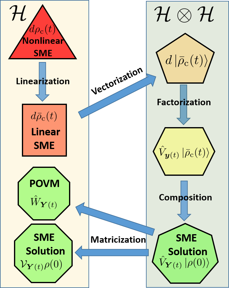
Figure 1: The sequence of steps involved in solving the SME and finding the POVM is schematically shown. Within the smaller polygons, the mathematical object that most closely matches the outcome of the process arrow labels is shown. Increasing side number of the polygon (together with shape color progression) represents sequential process steps, starting with the nonlinear SME and moving towards the twin goals of SME solution and obtaining the POVM. The two larger, enveloping, rectangles indicate whether the contained objects reside in the original Hilbert space, ${\cal H}$, or the enlarged Hilbert space, ${\cal H}\otimes{\cal H}.$

Given the task of solving the SME, one might initially begin by hoping to obtain the dynamical mapping, in the form of an evolution superoperator ${\cal N}_{{\bm{Y}}(t)}$, that evolves the initial state of the system, $\rho(0)$, to the final state, $\rho(t)$. The use of the subscript ${\bm{Y}}(t)$ is to indicate the set of measurement results obtained over the finite interval $[0,t]$, rather than the instantaneous results obtained at time $t$ (denoted by ${\bm{y}}(t)$). That is, we want to find

$${\cal N}_{{\bm{Y}}(t)}:\rho_{{\rm c}}(t)={\cal N}_{{\bm{Y}}(t)}\rho(0).$$ (17)

The mapping ${\cal N}_{{\bm{Y}}(t)}$ will be stochastic, due to its dependence upon the measurement results. In order for $\rho_{{\rm c}}(t)$ to be a normalized density matrix, the mapping ${\cal N}_{{\bm{Y}}(t)}$ is, in general, nonlinear. This makes the task of directly finding it intractable.

To avoid the nonlinearity imposed by Eq. (1), it is necessary to consider the linear SME Goetsch and Graham (1994); Wiseman (1996); Jacobs and Knight (1998). A linear formulation being possible is a general feature of quantum measurement theory, thus extending the linearity of the unconditioned ME. The ‘cost’ of formulating measurement dynamics in this manner is that the system state becomes unnormalised. The state norm has meaning, as will be specified later in this section. We term moving from the nonlinear to linear equation as ‘linearization’ of the SME, and associate with it the traceful incremental evolution $d\bar{\rho}_{{\rm c}}(t)$. To be clear, linearization is not an approximation in any sense; the linearized SME is as accurate as the nonlinear SME. The normalised density matrix is, of course, found from $\rho_{{\rm c}}(t)=\bar{\rho}_{{\rm c}}(t)/\operatorname{Tr}\left[\bar{\rho}_{{\rm c}}(t)\right]$. The overbar indicates an unnormalized state.

In order to deal with ordinary operators, rather than superoperators, step two of our solution method is to transform the linear SME for the unnormalized density matrix, $\bar{\rho}(t)$, into a linear equation for a state vector, $\left|\bar{\rho}(t)\right\rangle$ in a larger Hilbert space. This ‘vectorized’ equation in the larger Hilbert space would consist of left-only matrix multiplication of the state vector. For a finite dimensional basis, this can be achieved simply by column stacking the elements of $\rho$ to form a vector. That it can be achieved for infinite dimensional bosonic modes, via the thermo-entangled state representation Fan and Fan (1998); Arimitsu and Umezawa (1985); Umezawa et al. (1982) in a larger Hilbert space ${\cal H}\otimes{\cal H}$, will be discussed when the detailed solution method is provided in the next section. For the moment, we note that it is possible to recast the evolution $d\bar{\rho}_{{\rm c}}(t)$, via what we term ‘vectorization’, into $d\left|\bar{\rho}_{{\rm c}}(t)\right\rangle$.

Our goal is to obtain the mapping from $\left|\rho(0)\right\rangle$ to $\left|\bar{\rho}_{{\rm c}}(t)\right\rangle$. To achieve this, we first need to obtain the mapping corresponding to an infinitesimal time slice, $dt$,

$$\left|\bar{\rho}_{{\rm c}}(t+dt)\right\rangle = d\left|\bar{\rho}_{{\rm c}}(t)\right\rangle+\left|\bar{\rho}(t)\right\rangle$$ (18)

$$= \hat{V}_{{\bm{y}}(t)}\left|\bar{\rho}(t)\right\rangle,$$ (19)

where $\hat{V}_{{\bm{y}}(t)}$ represents nonunitary evolution. That $\hat{V}_{{\bm{y}}(t)}$ can be obtained from Eq. (18) is clear, given the linear form of the SME. However, it is also useful to put $\hat{V}_{{\bm{y}}(t)}$ in an exponential form,

$$\hat{V}_{{\bm{y}}(t)}=e^{\hat{v}_{{\bm{y}}(t)}},$$ (20)

for some operator $\hat{v}_{{\bm{y}}(t)}$, as this allows contact with techniques from Lie algebra. We refer to finding $\hat{V}_{{\bm{y}}(t)}$, and obtaining its desired form, as a process of ‘factorization’ (see Fig. 1).

The next step in obtaining the evolution operator for a finite time interval begins with the division of $t$ into a very large number, $J$, of time slices of length $dt$. The finite evolution is given by

$$\left|\bar{\rho}_{{\rm c}}(t)\right\rangle = \hat{V}_{{\bm{y}}(Jdt)}\cdots\hat{V}_{{\bm{y}}(2dt)}\hat{V}_{{\bm{y}}(dt)}\left|\rho(0)\right\rangle$$ (21)

$$\equiv \hat{V}_{{\bm{Y}}(t)}\left|\rho(0)\right\rangle.$$ (22)

By finding the nonunitary evolution operator, $\hat{V}_{{\bm{Y}}(t)}$, which depends on the set, ${\bm{Y}}(t)$, of all measurement results over the interval $[0,t]$, the evolution is solved. In the limit $dt\rightarrow 0$, $\hat{V}_{{\bm{Y}}(t)}$ will contain integrals over the measurement record. The process of finding $\hat{V}_{{\bm{Y}}(t)}$, from the string of operators representing infinitesimal evolution, is termed ‘composition’.

If desired, the vectorization to form $\left|\bar{\rho}_{{\rm c}}(t)\right\rangle$ can be unwound to write the solution in terms of $\bar{\rho}_{{\rm c}}(t)$. We refer to this unwinding as ‘matricization’ as we are moving from the state vector, in the larger Hilbert space, back to the state matrix, in the original Hilbert space. The density matrix SME solution, as opposed to the state vector, is written in terms of a evolution superoperator, ${\cal V}_{{\bm{Y}}(t)}$, analogous to the evolution operator:

$$\bar{\rho}_{{\rm c}}(t)={\cal V}_{{\bm{Y}}(t)}\rho(0).$$ (23)

Having sketched how to solve the SME, we now extend a little further and indicate how the POVM is subsequently obtained. The POVM, which characterizes a quantum measurement, is defined as the set of positive operators, $\{\hat{W}_{{\bm{Y}}(t)}:{\bm{Y}}(t)\}$, such that for all (normalized) $\rho(0)$

$$\wp_{{\bm{Y}}(t)}=\operatorname{Tr}[\hat{W}_{{\bm{Y}}(t)}\rho(0)],$$ (24)

where $\wp_{{\bm{Y}}(t)}$ is the probability density for the measurement record ${\bm{Y}}(t)$ and $\hat{W}_{{\bm{Y}}(t)}$ is known as the ‘effect’ operator.

As mentioned earlier, the norm of the system state vector, $\left\|\left|\bar{\rho}_{{\rm c}}(t)\right\rangle\right\|$, has meaning when an initially normalized state is evolved using the linear SME. Specifically, the norm is related to the probability of the measurement sequence, upon which the state is conditioned, as per

$$\wp_{{\bm{Y}}(t)}=\left\|\left|\bar{\rho}_{{\rm c}}(t)\right\rangle\right\|\wp_{{\rm ost}}({\bm{Y}}(t)).$$ (25)

There is some flexibility in the linear SME, relating to the choice of normalization. However, $\wp_{{\bm{Y}}(t)}$ is a fixed quantity, so variations in $\left\|\left|\bar{\rho}_{{\rm c}}(t)\right\rangle\right\|$ must be compensated by the form of the ‘ostensible distribution’, $\wp_{{\rm ost}}({\bm{Y}}(t))$ Wiseman and Milburn (2014). In this solution sketch, the specification of the particular form of the linear SME and ostensible distribution is not crucial, apart from noting that an analytic form can be found for both, and is left until later sections. The reader is invited to read Appendix A for a more detailed discussion of the ostensible distribution.

The form of $\hat{W}_{{\bm{Y}}(t)}$ is fixed by ensuring that the two expressions for $\wp_{{\bm{Y}}(t)}$, given in Eq. (24) and Eq. (25), are equal. The effect operator is an operator in the original sized Hilbert space, so it is necessary to revert from the larger Hilbert space, via ‘matricization’, when determining $\hat{W}_{{\bm{Y}}(t)}$. As indicated by Eq. (25), and shown in Fig. 1, we will find the POVM from $\left|\bar{\rho}_{{\rm c}}(t)\right\rangle$, the state vector form of the SME solution. However, this is a matter of convenience; the POVM can, of course, be found from the SME density matrix solution. The class of systems that we consider (those with linear HP dynamics and Gaussian measurement noise) will be found to have Gaussian effect operators. A Gaussian operator is one which has a Gaussian Wigner function.

IV Solving the stochastic master equation

IV.1 Linearization

In Sec. III, a sequence of steps, that leads to the solution of a SME, was identified. We now carry out these steps, beginning with the linearizing of the nonlinear SME. The nonlinear SME, for the system class of interest, has already been provided in Eq. (1). As explained in Appendix A, the nonlinearity of the SME only affects the normalization of the density matrix so that one can faithfully propagate an unnormalized system state, $\bar{\rho}(t)$ using only linear terms, with what is known as a linear SME Chia and Wiseman (2011):

$$d\bar{\rho}(t) = -i\left[\hat{H},\bar{\rho}(t)\right]dt+{\cal D}\left[\hat{{\bm{c}}}\right]\bar{\rho}(t)dt$$ (26)

$$+{\bm{y}}^{{\rm T}}(t)dt\bar{{\cal H}}\left[{\bm{M}}^{{\dagger}}\hat{{\bm{c}}}\right]\bar{\rho}(t),$$

where a linear form of the superoperator, ${\cal H}$, has been used

$$\bar{{\cal H}}\left[\hat{{\bm{c}}}\right]\rho\equiv\hat{{\bm{c}}}\rho+\rho\hat{{\bm{c}}}^{\ddagger}.$$ (27)

The bar on $d\bar{\rho}(t)$ is used to indicate a measurement-conditioned, unnormalized state, with the subscript ‘c’ dropped for simplicity. Note that the linear SME is written directly in terms of the measurement results ${\bm{y}}(t)$, which have the Gaussian statistics indicated by Eqs. (7)–(8).

IV.2 Vectorization

The next step in the solution process is comprised of transforming the linear SME for the unnormalized density matrix into a vector form, in a larger Hilbert space. The thermo-entangled state representation is now briefly reviewed, before being applied to the linear SME.

IV.2.1 A brief introduction to the thermo-entangled state representation

To work in the thermo-entangled state representation, for a system consisting of $N$ physical modes described by a Hilbert space, ${\cal H}$, an ancillary Hilbert space of equal dimension is introduced, $\tilde{{\cal H}}$, which houses unphysical modes. This representation is based on prior work by Takahashi and Umezawa, relating to thermo field dynamics Arimitsu and Umezawa (1985); Umezawa et al. (1982), in which a fictitious field is introduced in order to convert ensemble average calculations into equivalent pure state expressions. Here, we focus on just the results that we require, and the interested reader is referred to the available literature for more detail Zhou et al. (2011); Hu and Fan (2009); Fan and Lu (2007); Kosov (2016); Fan and Fan (1998); Arimitsu and Umezawa (1985); Umezawa et al. (1982); Fan and Hu (2008); Ban (2009).

For an arbitrary operator $\hat{A}$ acting on vectors of the Hilbert space ${\cal H}$, there is a ‘tilde conjugate’ operator $\tilde{A}$ that acts identically on vectors of the Hilbert space $\tilde{{\cal H}}$. Without loss of generality, we can define the relationship between tilde and non-tilde operators as Kosov (2016)

$$\hat{A}=A(\hat{{\bm{a}}},\hat{{\bm{a}}}^{\dagger}),\quad\tilde{A}=A^{*}\left(\tilde{{\bm{a}}},\tilde{{\bm{a}}}^{\dagger}\right).$$ (28)

Note that $\tilde{{\bm{a}}}=\left(\tilde{a}_{1},\tilde{a}_{2},...,\tilde{a}_{N}\right)^{\rm T\color[rgb]{0,0,0}}$ has been introduced, and that taking the tilde conjugate of a matrix does not alter its dimensions. This generalizes to the case where the object to be tilde-conjugated is itself a matrix of operators, $\hat{{\bm{A}}}={\bm{A}}(\hat{{\bm{a}}},\hat{{\bm{a}}}^{\dagger})$, and the the matrix dimensions are left unaltered:

$$\tilde{{\bm{A}}}={\bm{A}}{}^{*}(\tilde{{\bm{a}}},\tilde{{\bm{a}}}^{\dagger}).$$ (29)

The tilde and non-tilde annihilation and creation operators obey standard bosonic commutation relations:

$$\left[\hat{a}_{m},\hat{a}_{n}\right] = \left[\tilde{a}_{m},\tilde{a}_{n}\right]=0,$$ (30)

$$\left[\hat{a}_{m},\hat{a}_{n}^{{}^{\dagger}}\right] = \left[\tilde{a}_{m},\tilde{a}_{n}^{{}^{\dagger}}\right]=\delta_{mn},$$ (31)

$$\left[\hat{a}_{m},\tilde{a}_{n}\right] = \left[\hat{a}_{m},\tilde{a}_{n}^{{}^{\dagger}}\right]=0,$$ (32)

for $m,n\in\{1,\ldots,N\}$.

From Eq. (28), and the requirement that $(\tilde{A})^{\widetilde{}}=\hat{A}$, the following ‘tilde-conjugation’ rules may be inferred

$$\left(z_{1}\hat{A}_{1}+z_{2}\hat{A}_{2}\right)^{\widetilde{}}=z_{1}^{*}\tilde{A}_{1}+z_{2}^{*}\tilde{A}_{2},$$ (33)

$$\left(\hat{A}_{1}\hat{A}_{2}\right)^{\widetilde{}}=\tilde{A_{1}}\tilde{A_{2}},$$

$$(\hat{A}^{\dagger})^{\widetilde{}}=(\tilde{A})^{\dagger},$$

for complex numbers $z_{1},z_{2}$.

Similarly to multimode coherent states, the ‘mixed’-mode operator

$$\hat{{\bm{\beta}}}=\hat{{\bm{a}}}-\tilde{{\bm{a}}}^{\ddagger}$$ (34)

(recall our previous definition, applying equally to tilde operators, that $\hat{{\bm{a}}}^{\ddagger}\equiv\left(\hat{{\bm{a}}}^{{\rm T}}\right)^{{\dagger}}$) may be defined, which has eigenstates:

$$\hat{{\bm{\beta}}}\left|{\bm{\beta}}\right\rangle={\bm{\beta}}\left|{\bm{\beta}}\right\rangle,\quad\hat{{\bm{\beta}}}^{\dagger}\left|{\bm{\beta}}\right\rangle={\bm{\beta}}^{{\dagger}}\left|{\bm{\beta}}\right\rangle,\quad{\bm{\beta}}\in\mathbb{C}^{N}.$$ (35)

Note the use of the non-operator expression ${\bm{\beta}}^{{\dagger}}=\left({\bm{\beta}}^{*}\right)^{{\rm T}}$, where ${\bm{\beta}}$ is a vector of complex numbers. Like position or momentum eigenstates, the states $\left|{\bm{\beta}}\right\rangle$ are not normalizable. From Eq. (35) we deduce that

$$\hat{{\bm{a}}}\left|{\bm{\beta}}={\bm{0}}\right\rangle=\tilde{{\bm{a}}}^{\ddagger}\left|{\bm{\beta}}={\bm{0}}\right\rangle,\quad\hat{{\bm{a}}}^{\ddagger}\left|{\bm{\beta}}={\bm{0}}\right\rangle=\tilde{{\bm{a}}}\left|{\bm{\beta}}={\bm{0}}\right\rangle.$$ (36)

Going forward, the cumbersome notation of $\left|{\bm{\beta}}={\bm{0}}\right\rangle$, indicating the zero eigenvector of $\hat{{\bm{\beta}}}$, will be dropped and merely written as $\left|{\bm{0}}\right\rangle\equiv\left|{\bm{\beta}}={\bm{0}}\right\rangle$. To distinguish this zero-valued eigenvector of $\hat{{\bm{\beta}}}$ — which we will often refer to as the thermo-entangled state vacuum — from the $2N$-mode vacuum state of the Hilbert space ${\cal H}\otimes\tilde{{\cal H}}$, we will denote the latter by $\left|\mathbf{VAC}\right\rangle$.

A useful consequence of Eq. (36) is that for the arbitrary, non-tilde, operator $\hat{{\bm{A}}}={\bm{A}}(\hat{{\bm{a}}},\hat{{\bm{a}}}^{\dagger})$ (which acts as the identity on tilde modes),

$$\hat{{\bm{A}}}\left|{\bm{0}}\right\rangle=\tilde{{\bm{A}}}^{\ddagger}\left|{\bm{0}}\right\rangle.$$ (37)

For the special case in which $\hat{{\bm{A}}}$ is Hermitian, this relation simplifies further, to

$$\hat{{\bm{A}}}\left|{\bm{0}}\right\rangle=\tilde{{\bm{A}}}\left|{\bm{0}}\right\rangle.$$ (38)

It is shown in Fan and Fan (1998) that the thermo-entangled states are given by:

$$\left|{\bm{\beta}}\right\rangle=\exp\left(-\frac{\left|{\bm{\beta}}\right|^{2}}{2}+\hat{{\bm{a}}}^{\dagger}{\bm{\beta}}-{\bm{\beta}}^{{\dagger}}\tilde{{\bm{a}}}^{\ddagger}+\hat{{\bm{a}}}^{\dagger}\tilde{{\bm{a}}}^{\ddagger}\right)\left|\mathbf{VAC}\right\rangle.$$ (39)

For later use, we note that the thermo-entangled state vacuum is given in terms of the Hilbert space vacuum by

$$\left|{\bm{0}}\right\rangle\equiv\left|{\bm{\beta}}={\bm{0}}\right\rangle=\exp\left(\hat{{\bm{a}}}^{\dagger}\tilde{{\bm{a}}}^{\ddagger}\right)\left|\mathbf{VAC}\right\rangle,$$ (40)

which follows directly from Eq. (39). As an aside, the thermo-entangled states are precisely the common eigenstates of the relative co-ordinate and total momentum of two particles, which are central to the original Einstein, Podolsky and Rosen (EPR) scheme Hong-yi and Klauder (1994); Einstein et al. (1935).

The thermo-entangled states allow us to represent an $N$-mode system density matrix, $\rho$, by a vector, $\left|\rho\right\rangle$, in the larger $2N$-mode Hilbert-space, via

$$\left|\rho\right\rangle\equiv\rho\otimes\hat{{\bm{1}}}\left|{\bm{0}}\right\rangle,$$ (41)

where the $N$-mode identity is acting on the unphysical modes.

IV.2.2 Application of the thermo-entangled state representation

As previously indicated, we will work in the thermo-entangled state representation, whereby the state matrix is vectorized according to $\left|\bar{\rho}\right\rangle\equiv\bar{\rho}\otimes\hat{{\bm{1}}}\left|{\bm{0}}\right\rangle$. That is, Eq. (26) is simply right multiplied by $\left|{\bm{0}}\right\rangle$ and then the relations of Eqs. (28)–(29) and Eqs. (36)–(38) are used. It is found that

$$d\left|\bar{\rho}(t)\right\rangle = \bigg{[}\hat{S}\left[-i\hat{H}\right]dt+\hat{D}\left[\hat{{\bm{c}}}\right]dt$$ (42)

$$\quad+{\bm{y}}^{{\rm T}}(t)dt\hat{S}\left[{\bm{M}}^{{\dagger}}\hat{{\bm{c}}}\right]\bigg{]}\left|\bar{\rho}(t)\right\rangle.$$

The operator $\hat{D}\left[\hat{{\bm{c}}}\right]$ is defined to represent the unconditional decoherence terms

$$\hat{D}\left[\hat{{\bm{c}}}\right]=\tilde{{\bm{c}}}^{{\rm T}}\hat{{\bm{c}}}-{\textstyle\frac{1}{2}}\hat{{\bm{c}}}^{{\dagger}}\hat{{\bm{c}}}-{\textstyle\frac{1}{2}}\left(\hat{{\bm{c}}}^{{\dagger}}\hat{{\bm{c}}}\right)^{\sim},$$ (43)

and we have also introduced notation for the sum of an operator and its tilde conjugate:

$$\hat{S}\left[{\bm{M}}^{{\dagger}}\hat{{\bm{c}}}\right]={\bm{M}}^{{\dagger}}\hat{{\bm{c}}}+\left({\bm{M}}^{{\dagger}}\hat{{\bm{c}}}\right)^{\sim}.$$ (44)

The RHS of Eq. (42)’s being invariant under tilde conjugation ensures that the hermiticity of the density matrix is preserved. The vectorization step of the SME solution is now complete.

IV.3 Factorization

The next step is to factorize the evolution. From Eq. (42), an expression for $\hat{V}_{{\bm{y}}(t)}$, such that

$$\left|\bar{\rho}(t+dt)\right\rangle=\hat{V}_{{\bm{y}}(t)}\left|\bar{\rho}(t)\right\rangle,$$ (45)

is trivially given by

$$\hat{V}_{{\bm{y}}(t)}=\hat{{\bm{1}}}+\hat{S}\left[-i\hat{H}\right]dt+\hat{D}\left[\hat{{\bm{c}}}\right]dt+{\bm{y}}^{{\rm T}}(t)dt\hat{S}\left[{\bm{M}}^{{\dagger}}\hat{{\bm{c}}}\right],$$ (46)

with the $2N$-mode identity operator acting on all modes of the doubled Hilbert space.

In order to calculate an evolution operator using the techniques of Lie algebra, an exponential operator form, $\hat{V}_{{\bm{y}}(t)}=\exp(\hat{v}_{{\bm{y}}(t)})$, is required. An expression for $\hat{v}_{{\bm{y}}(t)}$, that provides a $\hat{V}_{{\bm{y}}(t)}$ accurate to $\mathcal{O}(dt)$, is formally achieved with

$$\hat{v}_{{\bm{y}}(t)} = \hat{S}\left[-i\hat{H}\right]dt+\hat{D}\left[\hat{{\bm{c}}}\right]dt-\frac{1}{2}\left({\bm{y}}^{{\rm T}}(t)dt\hat{S}\left[{\bm{M}}^{{\dagger}}\hat{{\bm{c}}}\right]\right)^{2}$$ (47)

$$+{\bm{y}}^{{\rm T}}(t)dt\hat{S}\left[{\bm{M}}^{{\dagger}}\hat{{\bm{c}}}\right].$$

To verify Eq. (47), the exponential form of $\hat{V}_{{\bm{y}}(t)}$ should be expanded to first order in $dt$ and compared with Eq. (46). This requires the inclusion of the second order contribution from ${\bm{y}}^{{\rm T}}(t)dt\hat{S}\left[{\bm{M}}^{{\dagger}}\hat{{\bm{c}}}\right]$, as it is of order $\sqrt{dt}$ due to Itô’s rule (see Eq. (8)). The same reasoning implies that $\left({\bm{y}}^{{\rm T}}(t)dt\hat{S}\left[{\bm{M}}^{{\dagger}}\hat{{\bm{c}}}\right]\right)^{2}$ is actually deterministic and equal to $\left(dt\hat{S}\left[{\bm{M}}^{{\dagger}}\hat{{\bm{c}}}\right]^{{\rm T}}\hat{S}\left[{\bm{M}}^{{\dagger}}\hat{{\bm{c}}}\right]\right)$, to first order in $dt$. Despite being deterministic, this term results from the presence of measurement.

The first three terms of $\hat{v}_{{\bm{y}}(t)}$, written on the first line of Eq. (47), are deterministic, as well as being quadratic in the annihilation and creation operators. The final term of Eq. (47) is stochastic. It is linear in the measurement results, and linear in the annihilation and creation operators. This motivates the simplifying expression

$$\hat{v}_{{\bm{y}}(t)}=\hat{Q}dt+d\hat{L}(t),$$ (48)

where $\hat{Q}$ contains terms that are time independent and quadratic, while $d\hat{L}$ contains stochastic, linear terms. In summary, the dynamical map of Eq. (45) is achieved by the nonunitary evolution operator

$$\hat{V}_{{\bm{y}}(t)}=\exp\left[\hat{Q}dt+d\hat{L}(t)\right],$$ (49)

with

$$\hat{Q} = \hat{S}\left[-i\hat{H}\right]+\hat{D}\left[\hat{{\bm{c}}}\right]-{\textstyle\frac{1}{2}}\hat{S}\left[{\bm{M}}^{{\dagger}}\hat{{\bm{c}}}\right]^{{\rm T}}\hat{S}\left[{\bm{M}}^{{\dagger}}\hat{{\bm{c}}}\right],$$ (50)

$$d\hat{L}(t) = {\bm{y}}^{{\rm T}}(t)dt\hat{S}\left[{\bm{M}}^{{\dagger}}\hat{{\bm{c}}}\right].$$ (51)

IV.4 Composition

Given the evolution operator, $\hat{V}_{{\bm{y}}(t)}$, which evolves the state vector forward a single time slice, the next task is to consider a sequence of them that evolves the initial state forward a finite duration:

$$\left|\bar{\rho}(t)\right\rangle = \hat{V}_{{\bm{y}}(Jdt)}\cdots\hat{V}_{{\bm{y}}(2dt)}\hat{V}_{{\bm{y}}(dt)}\left|\rho(0)\right\rangle,$$ (52)

$$= \prod\limits_{j=1}^{J}\exp\left[\hat{Q}dt+d\hat{L}(jdt)\right]\left|\rho(0)\right\rangle$$ (53)

$$= \hat{V}_{{\bm{Y}}(t)}\left|\rho(0)\right\rangle.$$ (54)

In the second expression, Eq. (53), in which the form of Eq. (48) has been used, $Jdt=t$ and the product is enumerated with $j$ increasing from right to left. Note that a normalized initial state has been assumed. The goal of the ‘composition’ step is to find the finite evolution operator, $\hat{V}_{{\bm{Y}}(t)}$. This expression for the state matrix (albeit in vectorized form) is analogous to that for the state vector obtained in Jacobs and Knight (1998), thus allowing a similar fundamental approach (but requiring different techniques).

To derive a practicable expression for $\hat{V}_{{\bm{Y}}(t)}$, the long sequence of $J$ exponential operators must be re-ordered and composed (which will involve integration for $dt\rightarrow 0$) so as to form a small number of terms. This is a task in bosonic algebra and methods of Lie groups are used.

IV.4.1 Lie algebra

To make contact with Lie algebra, note that $\hat{v}_{{\bm{y}}(t)}$ is comprised of terms that are at most quadratic in the $2N$-mode annihilation and creation operators. This is ensured by the assumption of linear HP dynamics (see Sec. II). Here is a list of all $(4N+1)(2N+1)$ such operators:

$$\{ \hat{1},\hat{a}_{m},\hat{a}^{\dagger}_{m},\tilde{a}_{m},\tilde{a}_{m}^{{}^{\dagger}},$$ (55)

$$\hat{a}_{m}\hat{a}_{n},\tilde{a}_{m}\tilde{a}_{n},\hat{a}_{m}^{\dagger}\hat{a}_{n}^{\dagger},\tilde{a}_{m}^{\dagger}\tilde{a}_{n}^{\dagger},$$

$$\hat{a}_{m}\tilde{a}_{n},\hat{a}_{m}^{\dagger}\tilde{a}_{n}^{\dagger},\hat{a}_{m}\tilde{a}_{n}^{\dagger},\hat{a}_{m}^{\dagger}\tilde{a}_{n},$$

$$\hat{a}_{m}^{\dagger}\hat{a}_{n}+{\textstyle\frac{1}{2}}\delta_{mn},\tilde{a}_{m}^{\dagger}\tilde{a}_{n}+{\textstyle\frac{1}{2}}\delta_{mn}\},$$

for $m,n\in\{1,\ldots,N\}$. It is important to emphasize that unphysical tilde modes (represented by operators $\tilde{{\bm{a}}},\tilde{{\bm{a}}}^{{\dagger}}$) are on the same footing as physical modes (represented by operators $\hat{{\bm{a}}},\hat{{\bm{a}}}^{{\dagger}}$) in terms of bosonic algebra calculations.

The span over $\mathbb{C}$ of the operators is a subalgebra of the symplectic algebra $\mathfrak{sp}(4N+2)$ Gilmore and Yuan (1989); Zhang et al. (1990). The operator commutator is the Lie bracket for the Lie algebra. The Lie algebra, $\mathfrak{g}$, has an associated Lie group, $G$, that is formed by taking the exponential map of $\mathfrak{g}$,

$$g=\exp(X),$$ (56)

for $X\in\mathfrak{g}$ and $g\in G$. It can be seen that $\hat{v}_{{\bm{y}}(t)}\in\mathfrak{g}$ and it will become clear that $\hat{V}_{{\bm{Y}}(t)}\in G$. It is important to be clear that $\mathfrak{g}$ consists of arbitrary linear combinations of the operators listed in Eq. (55).

Of central importance to us is that there are group-theoretic calculations that are: (1) only dependent upon the algebra’s commutation relations, and (2) are independent of the representation that the calculations are carried out in, provided that the representation respects the algebra’s commutation relations Gilmore and Yuan (1987). In particular, this holds for multiplication within the group, and the related tasks of exponential operator disentanglement and reordering. As $\hat{V}_{{\bm{Y}}(t)}$ is formed through group multiplication, it follows that $\hat{V}_{{\bm{Y}}(t)}\in G$.

In the context of a Lie group, disentanglement refers to the splitting of an exponential operator, whose exponent consists of multiple terms, into a product of exponential operators. That is, for $Z\in\mathfrak{g}$ we disentangle the exponential operator into a product of $n$ terms as per

$$e^{Z}=e^{X_{1}}\ldots e^{X_{n}},$$ (57)

for $X_{1},\ldots,X_{n}\in\mathfrak{g}$. To give an illustrative example, a simple, but well-known, disentanglement is the normal-ordering of the single-mode displacement operator

$$e^{\alpha\hat{a}^{{\dagger}}-\alpha^{*}\hat{a}}=e^{\alpha\hat{a}^{{\dagger}}}e^{-\alpha^{*}\hat{a}}e^{-\frac{1}{2}\left|{\alpha}\right|^{2}},$$ (58)

for $Z=\alpha\hat{a}^{{\dagger}}-\alpha^{*}\hat{a}$. This disentanglement follows directly from the Zassenhaus formula Wilcox (1967)

$$e^{X+Y}=e^{X}e^{Y}e^{-{\textstyle\frac{1}{2}}[X,Y]}\cdots,$$ (59)

with further terms in the product containing higher order commutators, for example $[Y,[X,Y]]$. In the case of the displacement operator, the higher order commutators evaluate to zero. It is important to note that algebra described by Eq. (55) is significantly more complicated than that of the subalgebra, $\{\hat{1},\hat{a},\hat{a}^{{\dagger}}\}$, relevant to the displacement operator, and we will not in general use the Zassenhaus formula to evaluate disentanglements. Despite this, the Zassenhaus formula highlights that disentanglement is only dependent upon the commutation relations of the algebra.

The second group-theoretic calculation of importance to us is exponential operator reordering. Given the operator $e^{X}e^{Y}$, we may wish to write an equivalent expression in which the $e^{Y}$ term appears to the left. That is,

$$e^{X}e^{Y}=e^{Y}e^{Z},$$ (60)

for known $X,Y\in\mathfrak{g}$ and a to-be-determined $Z=e^{-Y}e^{X}e^{Y}\in\mathfrak{g}$. It is possible to give an expression for $Z$ Hall (2015),

$$Z=X-[Y,X]+\frac{1}{2!}[Y,[Y,X]]+\ldots,$$ (61)

which makes it clear that operator reordering is a function of the group commutation relations only.

Having established the central role that the commutator plays in operator reordering and disentanglement, we are motivated to look at the commutator structure of the Lie algebra, $\mathfrak{g}$. To do so we define a number of partially overlapping subalgebras. We define the subalgebra $\mathfrak{q}$ as containing all the quadratic (in annihilation and creation operators) elements of $\mathfrak{g}$, together with the identity operator. Similarly, the subalgebra $\mathfrak{l}$ is defined as containing all linear elements of $\mathfrak{g}$, together with the identity. Finally, we define $\mathfrak{i}$ as the subalgebra consisting only of the identity operator. Then, we note the following useful facts:

$$[\mathfrak{q},\mathfrak{q}]\in\mathfrak{q},$$ (62)

$$[\mathfrak{l},\mathfrak{g}]\in\mathfrak{l},$$ (63)

$$[\mathfrak{l},\mathfrak{l}]\in\mathfrak{i},$$ (64)

$$[\mathfrak{l},[\mathfrak{l},\mathfrak{l}]]=0.$$ (65)

That is, $\mathfrak{q}$ forms a subalgebra of $\mathfrak{g}$, and $\mathfrak{l}$ is an ideal of $\mathfrak{g}$. Eq. (65) follows from Eq. (64) as the identity commutes with every algebra element (it is the center of the algebra), but we state it explicitly for the reader due to its frequent application.

The consequences of the algebraic facts of Eqs. (62)–(63) at the group level are the following. Given Eq. (57) for $Z\in\mathfrak{q}$, it is true that $X_{1},\ldots,X_{n}\in\mathfrak{q}$. That is, the disentanglement of the exponential of a quadratic operator is given by a product of exponentials that do not involve any linear exponents. Additionally, given Eq. (60) for $X\in\mathfrak{q}$ and $Y\in\mathfrak{l}$, then $Z\in\mathfrak{l}$. That is, when an exponential operator with quadratic exponent is moved through an exponential with linear exponent, the quadratic exponential is unchanged. The exponential with linear exponent retains a linear exponent only, but one that is changed according to Eq. (61).

As mentioned, we will not use the Zassenhaus formula, or Eq. (61), to calculate operator disentanglements and reordering for general elements $g\in G$. The algebra of $\mathfrak{g}$ is, in general, too complicated to make this feasible. Instead, we use the fact that a representation of the algebra that upholds the algebra’s commutation relations can be employed to perform group calculations, with the results then abstracted back to the level of the algebra. To make the representation-independent calculations, it is beneficial to choose as simple as possible a representation that faithfully respects the algebra $\mathfrak{g}$. The bosonic operators of $\mathfrak{g}$ are typically represented in the infinite dimensional Fock basis, but this is an unnecessary complication as far as group calculation is concerned. It is a convenient fact that there exist faithful finite dimensional matrix representations of $\mathfrak{g}$. All such faithful finite dimensional matrix representations are known, with the smallest using matrices of dimension $(4N+2)\times(4N+2)$ in order to represent the $2N$-mode algebra, $\mathfrak{g}$, of Eq. (55) Gilmore (2012, 2012); Gilmore and Yuan (1989). As a reminder, this $2N$-mode algebra corresponds to $N$ physical modes as well as $N$ unphysical modes that were introduced to facilitate the vectorization of the SME.

Let us now assume, as will be true in practice, that we have chosen the minimally sized $(4N+2)$ matrices to represent the algebra $\mathfrak{g}$. This leads to the disentanglement and operator reordering equations, Eqs. (57)–(60), being represented as matrix equations. In other words, to find the parameters which describe the disentanglement and reordering, a finite set of algebraic equations needs solving. To construct these equations requires the exponentiation of symbolic matrices; for our systems this involves solving polynomials of degree $2N$. As no known general solution exists for polynomials of degree higher than quartic, this approach has some intrinsic limitations for greater than two physical modes. Despite this, the Lie algebra facts detailed in this section will provide useful information regarding the form of the solution of the SME for arbitrary $N$, as well as more explicit results for $N\leq 2$. Finite dimensional matrix representations, and how they can be utilized in our calculations, are discussed further in Appendix B. We prefer to defer explicit finite dimensional matrix calculations to appendices in order to improve the readability of the main text.

Having described the essential techniques of Lie algebra, we can now return to the composition of the nonunitary evolution operator, $\hat{V}_{{\bm{Y}}(t)}$.

IV.4.2 Evolution operator form

In the remainder of this section, we will be heuristic in our calculations. The reason for this is that the details will likely not add significantly to the conceptual understanding gained by the reader. Despite this, the practical implementation of our SME solutions is obviously important, so we provide a recipe for their use in Sec. VI, as well as examples in Sec. VII. The reader will also be referred to appendices as appropriate. In this subsection, we obtain the form of the evolution operator $\hat{V}_{{\bm{Y}}(t)}$.

Before reordering the product of exponential terms in Eq. (53), we perform the simple disentanglement of splitting the quadratic and linear terms that belong to each time slice. That is,

$$\hat{V}_{{\bm{y}}(t)} = \exp\left[\hat{Q}dt+d\hat{L}(t)\right]$$ (66)

$$= \exp\left[d\hat{L}(t)\right]\exp\left[\hat{Q}dt\right],$$ (67)

which is correct up to order $dt$. This can be seen from Eq. (59), as the corrections involve commutators of the infinitesimal operators. For example, $[\hat{Q}dt,d\hat{L}(t)]={\cal O}(dt^{3/2})$.

The general strategy to find $\hat{V}_{{\bm{Y}}(t)}$ begins with moving the rightmost quadratic exponential through the linear exponential to its left not . After this is done, it is in contact with a second quadratic exponential, with which it can be combined,

$$\exp\left[\hat{Q}dt\right]\exp\left[\hat{Q}dt\right]=\exp\left[2\hat{Q}dt\right],$$ (68)

as the exponents obviously commute for our time-independent $\hat{Q}$. This combined quadratic exponential is then moved through the next linear exponential to the left and combined with a third quadratic exponential. After this has been repeated $j-1$ times, the task of reordering the combined quadratic exponential with the next linear exponential is given by

$$e^{d\hat{L}(jdt)}\prod\limits_{k=1}^{j}\exp\left[\hat{Q}dt\right] = e^{d\hat{L}(\tau)}e^{\hat{Q}\tau}$$ (69)

$$= e^{\hat{Q}\tau}e^{d\hat{L}^{\prime}(\tau)},$$ (70)

with the interim time $jdt$ labeled as $\tau$. The reordering, performed in Eq. (70), is an example of the reordering shown in Eq. (60) for $Y\in\mathfrak{q}$ and $X\in\mathfrak{l}$. As described in the previous subsection, the quadratic exponential is left unchanged while the linear exponential remains linear but is modified. The use of the prime in Eq. (70), for the linear exponential, is to indicate this modification. Following the movement of the quadratic exponentials through all the linear exponentials, we are left with

$$\hat{V}_{{\bm{Y}}(t)}=e^{\hat{Q}t}\prod\limits_{j=1}^{J}\exp\left[d\hat{L}^{\prime}(jdt)\right].$$ (71)

Next, we wish to combine all the linear exponentials. We note that $d\hat{L}^{\prime}(jdt)\in\mathfrak{l}$. Thus, according to Eq. (59) and Eqs. (64)–(65), we can write

$$\prod\limits_{j=1}^{J}\exp\left[d\hat{L}^{\prime}(jdt)\right]=\exp\left[\delta_{{\bm{Y}}(t)}\hat{1}+\sum_{j=1}^{J}d\hat{L}^{\prime}(jdt)\right],$$ (72)

with $\delta_{{\bm{Y}}(t)}$ being a scalar that is a function of the stochastic measurement record. From this point onward, the identity operator is not explicitly written, due to its trivial action. For convenience, we combine the linear term and that proportional to the identity into a single operator as per

$$\hat{L}^{\prime}(t)=\delta_{{\bm{Y}}(t)}+\sum_{j=1}{J}d\hat{L}^{\prime}(jdt),$$ (73)

where $\hat{L}^{\prime}(t)$ is finite and will convert into a stochastic Itô integral in the limit $dt\rightarrow 0$. The $\delta_{{\bm{Y}}(t)}$ term does not affect the system state, but is relevant to the probability of obtaining the measurement record (see Eq. (25)).

We can now give the form of $\hat{V}_{{\bm{Y}}(t)}$ as

$$\hat{V}_{{\bm{Y}}(t)}=e^{\hat{Q}t}e^{\hat{L}^{\prime}(t)}.$$ (74)

As desired, the evolution operator has been composed into a product of a finite number of exponentials (in this case, two). The first is deterministic and contains quadratic operator terms. The second is linear and is a function of the measurement record. When $\hat{V}_{{\bm{Y}}(t)}$ is used in Eq. (54), the solution of the SME,

$$\left|\bar{\rho}(t)\right\rangle=e^{\hat{Q}t}e^{\hat{L}^{\prime}(t)}\left|\rho(0)\right\rangle,$$ (75)

is obtained. Note that the invariance of $\hat{V}_{{\bm{Y}}(t)}$ under tilde conjugation, $\hat{V}_{{\bm{Y}}(t)}=\tilde{V}_{{\bm{Y}}(t)}$, ensures that $\bar{\rho}(t)$ is Hermitian. In the next two subsections we will provide more detail concerning $\hat{L}^{\prime}(t)$ and find a more convenient expression for $e^{\hat{Q}t}$.

IV.4.3 Investigating $e^{\hat{L}^{\prime}(t)}$

In this subsection, we give expressions for $e^{\hat{L}^{\prime}(t)}$ that will be of later use, with calculational details deferred to appendices. For notational convenience, and to emphasize that unphysical tilde modes are on the same footing as physical modes in terms of bosonic algebra calculations, the $\hat{{\bm{a}}}$ and $\tilde{{\bm{a}}}$ column vectors are placed into a single column vector of length $2N$:

$$\hat{{\bm{b}}}=\left(\hat{{\bm{a}}};\tilde{{\bm{a}}}\right)=\left(\hat{a}_{1},...,\hat{a}_{N},\tilde{a}_{1},...,\tilde{a}_{N}\right)^{T}.$$ (76)

We can now write $\hat{Q}$ and $d\hat{L}(t)$ in terms of the bosonic vector $\hat{{\bm{b}}}$:

$$\hat{Q}t= \hat{{\bm{b}}}^{{\dagger}}{\bm{R}}\hat{{\bm{b}}}^{\ddagger}+\hat{{\bm{b}}}^{{\dagger}}{\bm{D}}\hat{{\bm{b}}}+\hat{{\bm{b}}}^{{\rm T}}{\bm{L}}\hat{{\bm{b}}}$$ (77)

$$d\hat{L}(t)= \hat{{\bm{b}}}^{{\dagger}}d{\bm{r}}+d{\bm{l}}\hat{{\bm{b}}},$$ (78)

with the $2N\times 2N$ matrices ${\bm{R}},{\bm{D}},{\bm{L}}$, the $2N\times 1$ column vector, $d{\bm{r}}$, and the $1\times 2N$ row vector, $d{\bm{l}}$, all constrained by Hermiticity preservation of the evolved state matrix. Rather than use $\left\{{\bm{r}},{\bm{l}}\right\}$ we have introduced $\left\{d{\bm{r}},d{\bm{l}}\right\}$, in the linear evolution containing the measurement noise, to emphasize that they are infinitesimal and are of $\mathcal{O}(\sqrt{dt})$. The relationship between the system description in Eq. (26), that is given in terms of $\{{\bm{G}},{\bm{C}},{\bm{M}}\}$, and the parameterization of $\{{\bm{R}},{\bm{D}},{\bm{L}},d{\bm{l}},d{\bm{r}}\}$ of Eqs. (77)–(78) is provided in Appendix C. Note that $d\hat{L}^{\prime}(t)$ is defined analogously to Eq. (78), in terms of $\{d{\bm{r}}^{\prime},d{\bm{l}}^{\prime}\}$ (see Eq. (265)).

The explicit expression for $\hat{L}^{\prime}(t)$ is not difficult to derive using a finite dimensional representation of the algebra $\mathfrak{sp}(4N+2)$ (see Appendix B for details of this calculation, in particular Appendix B.3.1 and Appendix B.3.2). In this section we state it as

$$e^{\hat{L}^{\prime}(t)}=e^{h}e^{\hat{{\bm{b}}}^{{\dagger}}{\bm{r}}^{\prime}}e^{{\bm{l}}^{\prime}\hat{{\bm{b}}}},$$ (79)

with $h$ being a scalar non-Gaussian complex-valued stochastic integral and

$${\bm{r}}^{\prime}(\tau) = \int\limits_{0}^{\tau}d{\bm{r}}^{\prime}(s),$$ (80)

with equivalent notation for ${\bm{l}}^{\prime}(\tau)$. The explicit time dependence of $\{{h,\bm{l}}^{\prime},{\bm{r}}^{\prime}\}$ in Eq. (79) has been suppressed for display purposes. The relevance (or lack thereof) of the presence of the non-Gaussian random variable, $h$, will be discussed in detail in relation to the POVM, in Sec. V. For the moment we note that $h$ has no effect upon the system state, as the non-operator multiplicative factor, $e^{h}$, will be removed when the state is normalized. In other words, rather than storing the entire measurement record, ${\bm{Y}}(t)$, it is sufficient to track only $\{{\bm{l}}^{\prime},{\bm{r}}^{\prime}\}$ in order to follow the system state. In closing this subsection, we remind the reader that $e^{\hat{L}^{\prime}(t)}$ is the only term in our SME solution impacted explicitly by the measurement record.

IV.4.4 Disentangling $e^{\hat{Q}t}$

In order to facilitate calculations, such as expectation values, it is often convenient to use a disentangled exponential operator, with an ordering chosen to suit the calculation. In this subsection, we give the disentangled form of $e^{\hat{Q}t}$. This should be understood in the context of Eq. (57) for $Z,X_{1},\ldots,X_{n}\in\mathfrak{q}$. That is, we split $e^{\hat{Q}t}$ into a product of exponentials with quadratic (and no linear) exponents. Once again, only the heuristic form is provided in this section as the explicit results are obtained from the finite dimensional representation of $\mathfrak{sp}(4N+2)$ (see Appendix B, together with Sec. VI for details and examples). Using the form of $\hat{Q}$ given in Eq. (77) we state

$$e^{\hat{Q}t}= \exp\left[\hat{{\bm{b}}}^{{\dagger}}{\bm{R}}\hat{{\bm{b}}}^{\ddagger}+\hat{{\bm{b}}}^{{\dagger}}{\bm{D}}\hat{{\bm{b}}}+\hat{{\bm{b}}}^{{\rm T}}{\bm{L}}\hat{{\bm{b}}}\right]$$ (81)

$$= e^{\delta^{\prime}}\exp\left[\hat{{\bm{b}}}^{{\dagger}}{\bm{R}}^{\prime}\hat{{\bm{b}}}^{\ddagger}\right]\exp\left[\hat{{\bm{b}}}^{{\dagger}}\underline{{\bm{D}}}\hat{{\bm{b}}}\right]\exp\left[\hat{{\bm{b}}}^{{\rm T}}{\bm{L}}^{\prime}\hat{{\bm{b}}}\right]$$ (82)

$$= e^{\delta^{\prime}}\exp\left[\hat{{\bm{b}}}^{{\dagger}}{\bm{R}}^{\prime}\hat{{\bm{b}}}^{\ddagger}\right]\left(:\exp\left[\hat{{\bm{b}}}^{{\dagger}}{\bm{D}}^{\prime}\hat{{\bm{b}}}\right]:\right)\exp\left[\hat{{\bm{b}}}^{{\rm T}}{\bm{L}}^{\prime}\hat{{\bm{b}}}\right],$$ (83)

with the primes and underline indicating different functions of system parameters. Also, ${\bm{D}}^{\prime}=e^{\underline{\bm{D}}}-{\bm{1}}_{2N}$ by a standard operator identity for normal ordering H-Y (1989). Note the appearance of the scalar $\delta^{\prime}$, due to the disentanglement involving the commutation of quadratic terms.

We have now solved the linear SME in the enlarged Hilbert space, ${\cal H}\otimes\tilde{{\cal H}}$. The solution is comprised of Eq. (75), Eq. (79) and Eq. (82), together with the explicit expressions for primed variables contained in Appendix B. Some readers will object to the presence of the unphysical tilde modes, but we note that there are advantages in the thermo-entangled state representation of the solution. For example, to find expectation values of a system operator $A(\hat{{\bm{a}}},\hat{{\bm{a}}}^{\dagger})$ we use Fan and Lu (2007)

$$\operatorname{Tr}[A(\hat{{\bm{a}}},\hat{{\bm{a}}}^{\dagger})\bar{\rho}(t)]=\left\langle{\bm{0}}\left|A(\hat{{\bm{a}}},\hat{{\bm{a}}}^{\dagger})\right|\bar{\rho}(t)\right\rangle.$$ (84)

As the system state is mixed in general (that is, impure) we cannot separately factorize the exponentials of physical and unphysical mode operators. The conversion of the state vector, $\left|\bar{\rho}(t)\right\rangle$, to the state matrix, $\bar{\rho}(t)$, will necessitate the use of superoperators instead of operators or, alternatively, the power series expansion of exponentials. Indeed, when finding the POVM representing the composite measurement, we find it more simple to use the $\left|\bar{\rho}(t)\right\rangle$ solution. However, it is of clear relevance to show that we can find $\bar{\rho}(t)$, so this is performed in the next subsection.

For completeness, we perform one final operator reordering, being that of normal ordering the full evolution operator. That is

$$\hat{V}_{{\bm{Y}}(t)} = e^{\hat{Q}t}e^{\hat{L}^{\prime}(t)}$$ (85)

$$= e^{h+\delta^{\prime}}e^{\hat{{\bm{b}}}^{{\dagger}}\underline{{\bm{r}}}+\hat{{\bm{b}}}^{{\dagger}}{\bm{R}}^{\prime}\hat{{\bm{b}}}^{\ddagger}}\left(:e^{\hat{{\bm{b}}}^{{\dagger}}{\bm{D}}^{\prime}\hat{{\bm{b}}}}:\right)e^{\hat{{\bm{b}}}^{{\rm T}}{\bm{L}}^{\prime}\hat{{\bm{b}}}+\underline{{\bm{l}}}\hat{{\bm{b}}}},$$ (86)

where the reordering has lead to modification of the linear terms from $\{{\bm{l}}^{\prime},{\bm{r}}^{\prime}\}$ to $\{\underline{{\bm{l}}},\underline{{\bm{r}}}\}$, as detailed in Appendix B.3.3.

IV.5 Matricization

The solution $\left|\bar{\rho}(t)\right\rangle$ is a vector in ${\cal H}\otimes\tilde{{\cal H}}$ and contains the unphysical mode operators $\tilde{{\bm{a}}}$ and $\tilde{{\bm{a}}}^{\dagger}$ (within the mixed mode operators $\hat{{\bm{b}}}$ and $\hat{{\bm{b}}}^{{\dagger}}$). These can be removed in the following way. Recall that $\left|\rho(0)\right\rangle\equiv\rho(0)\otimes\hat{{\bm{1}}}\left|\bm{0}\right\rangle$, where $\rho(0)$ is the physical mode density matrix. All tilde mode operators commute through $\rho(0)$ to act on $\left|\bm{0}\right\rangle$, with the conversion to physical mode operators as per Eq. (36).

To identify the tilde mode operators, the compactifying notation of the the $\hat{{\bm{b}}}$ operators is unwound. As should be evident already, there are an endless number of operator orderings that can be chosen, each with a parameterization. To avoid having to repeat the definition, we note that for all $\{{\bm{R}},{\bm{L}},{\bm{D}},{\bm{r}},{\bm{l}}\}$ matrices (including $\{\underline{\bm{R}},\underline{\bm{L}},\underline{\bm{D}},\underline{\bm{r}},\underline{\bm{l}}\}$ and $\{{\bm{R}}^{\prime},{\bm{L}}^{\prime},{\bm{D}}^{\prime},{\bm{r}}^{\prime},{\bm{l}}^{\prime}\}$ or any other disentanglement parameters), the following block form will hold

$${\bm{L}} = \left[\begin{array}[]{cc}{\bf L}&\breve{{\bf L}}\\ \breve{{\bf L}}&{\bf L}^{*}\end{array}\right]$$ (89)

$${\bm{R}} = \left[\begin{array}[]{cc}{\bf R}&\breve{{\bf R}}\\ \breve{{\bf R}}&{\bf R}^{*}\end{array}\right],$$ (92)

$${\bm{D}} = \left[\begin{array}[]{cc}{\bf D}&\breve{{\bf D}}\\ \breve{{\bf D}}^{*}&{\bf D}^{*}\end{array}\right],$$ (95)

with $\breve{{\bf R}}=\breve{{\bf R}}^{{}^{\dagger}}=\breve{{\bf R}}^{{\rm T}}$ and ${\bf R}={\bf R}^{{\rm T}}$. The same respective properties hold for $\{{\bf L},\breve{{\bf L}}\}$, but not necessarily for the block matrices of ${\bm{D}}$. The vectors $\{{\bm{l}},{\bm{r}}\}$ (and operator reordered variations) all have the block form

$${\bm{l}} = \left[\begin{array}[]{cc}{{\bf l}}&{{\bf l}}^{*}\end{array}\right],$$ (97)

$${\bm{r}} = \left[\begin{array}[]{c}{{\bf r}}\\ {{\bf r}}^{*}\end{array}\right].$$ (100)

The requirement that evolution preserves state matrix hermiticity has been enforced for all parameters. Note that Roman font has been used to distinguish the $N\times N$ block matrices from the full matrix (which is $2N\times 2N$), and similarly for the block vectors of length $N$ rather than $2N$. To give an example to illustrate our notation, we have implied that the block form of $\{{\bm{R}}^{\prime},{\bm{D}}^{\prime}\}$ is

$${\bm{R}}^{\prime} = \left[\begin{array}[]{cc}{\bf R}^{\prime}&\breve{{\bf R}}^{\prime}\\ \breve{{\bf R}}^{\prime}&{\bf R}^{\prime*}\end{array}\right],$$ (103)

$${\bm{D}}^{\prime} = \left[\begin{array}[]{cc}{\bf D}^{\prime}&\breve{{\bf D}}^{\prime}\\ \breve{{\bf D}}^{\prime*}&{\bf D}^{\prime*}\end{array}\right],$$ (106)

with $\breve{{\bf R}^{\prime}}=\breve{{\bf R}}^{\prime^{\dagger}}=\breve{{\bf R}}^{\prime{\rm T}}$ and ${\bf R}^{\prime}={\bf R}^{\prime{\rm T}}$.

By substituting the block form of Eqs. (89)–(100) into Eq. (86), one can obtain an expression for $\hat{V}_{{\bm{Y}}(t)}$ in terms of $\{\hat{{\bm{a}}},\hat{{\bm{a}}}^{{}^{\dagger}},\tilde{{\bm{a}}}^{{\dagger}},\tilde{{\bm{a}}}^{{\dagger}}\}$, rather than $\{\hat{{\bm{b}}},\hat{{\bm{b}}}^{{\dagger}}\}$. This gives a lengthy, but useful, aid for moving to the state matrix solution of the linear SME:

$$\hat{V}_{{\bm{Y}}(t)}=$$

$$\exp\left[\hat{{\bm{a}}}^{{}^{\dagger}}\underline{\bf r}+\tilde{{\bm{a}}}^{{}^{\dagger}}\underline{\bf r}^{*}+\hat{{\bm{a}}}^{{}^{\dagger}}{\bf R}^{\prime}\hat{{\bm{a}}}^{\ddagger}+\tilde{{\bm{a}}}^{{}^{\dagger}}{\bf R}^{\prime*}\tilde{{\bm{a}}}^{\ddagger}+2\hat{{\bm{a}}}^{{}^{\dagger}}\breve{{\bf R}}^{\prime}\tilde{{\bm{a}}}^{\ddagger}\right]$$

$$\times e^{\hat{{\bm{a}}}^{{}^{\dagger}}\underline{\breve{{\bf D}}}\tilde{{\bm{a}}}+\tilde{{\bm{a}}}^{{}^{\dagger}}\underline{\breve{{\bf D}}}^{*}\hat{{\bm{a}}}}e^{\hat{{\bm{a}}}^{{}^{\dagger}}\underline{\bf D}\hat{{\bm{a}}}}e^{\tilde{{\bm{a}}}^{{}^{\dagger}}\underline{\bf D}^{*}\tilde{{\bm{a}}}}\times$$

$$\exp\left[\hat{{\bm{a}}}^{{\rm T}}{\bf L}^{\prime}\hat{{\bm{a}}}+\tilde{{\bm{a}}}^{{\rm T}}{\bf L}^{\prime*}\tilde{{\bm{a}}}+2\hat{{\bm{a}}}^{{\rm T}}\breve{{\bf L}}^{\prime}\tilde{{\bm{a}}}+\underline{\bf l}\hat{{\bm{a}}}+\underline{\bf l}^{*}\tilde{{\bm{a}}}\right],$$ (107)

which manifestly preserves state matrix Hermiticity. Note that we choose to use the underlined operator ordering $e^{\hat{{\bm{b}}}^{{\dagger}}\underline{\bm{D}}\hat{{\bm{b}}}}$ rather than the primed normal odering $:e^{\hat{{\bm{b}}}^{{\dagger}}{\bm{D}}^{\prime}\hat{{\bm{b}}}}:$ for this purpose. After the tilde operators are moved through $\rho(0)$ to act on $\left|\bm{0}\right\rangle$, they become right-multiplying operators onto $\rho(0)$.

Our first option for representing the state matrix solution, $\bar{\rho}(t)$, is to place it in superoperator form

$$\bar{\rho}(t)={\cal V}_{{\bm{Y}}(t)}\rho(0).$$ (108)

We find it necessary to introduce new superoperators, as well as clarifying how superoperator matrix-multiplication functions. Our new superoperators, for an arbitrary vector of operators, $\hat{{\bm{c}}}$, and square matrix ${\bm{M}}$ (of the same length as $\hat{{\bm{c}}}$), are

$${\cal J}[\hat{{\bm{c}}}^{{\rm T}}]{\bm{M}}\rho = \hat{{\bm{c}}}_{i}^{{\rm T}}{\bm{M}}_{ij}\rho\hat{{\bm{c}}}_{j}^{{}^{\dagger}}$$ (109)

$${\cal K}[\hat{{\bm{c}}}^{{\rm T}}]{\bm{M}}\rho = \hat{{\bm{c}}}_{i}^{{\rm T}}{\bm{M}}_{ij}\rho\hat{{\bm{c}}}_{j}.$$ (110)

Thus, although ${\cal J}[\hat{{\bm{c}}}^{{\rm T}}]{\bm{M}}$ appears to be a row-vector, when acted upon an operator we define it so that it produces a scalar operator. This convention is used for all superoperators and shows how the right-multiplying operator indices are summed with the left-multiplying portion. We also use the superoperator $\bar{\cal H}$ from Eq. (27). We can then write

$${\cal V}_{{\bm{Y}}(t)} = \exp\left[\bar{{\cal H}}\left[\hat{{\bm{a}}}^{{}^{\dagger}}\underline{\bf r}+\hat{{\bm{a}}}^{{}^{\dagger}}{\bf R}^{\prime}\hat{{\bm{a}}}^{\ddagger}\right]+2{\cal J}\left[\hat{{\bm{a}}}^{{}^{\dagger}}\right]\breve{{\bf R}}^{\prime}\right]\times$$ (111)

$$\exp\left[{\cal K}\left[\hat{{\bm{a}}}^{{}^{\dagger}}\right]\underline{\breve{{\bf D}}}+{\cal K}\left[\hat{{\bm{a}}}^{{\rm T}}\right]\underline{\breve{{\bf D}}}^{{}^{\dagger}}\right]\exp\left[\bar{\cal H}\left[\hat{{\bm{a}}}^{{}^{\dagger}}\underline{{\bf D}}\hat{{\bm{a}}}\right]\right]\times$$

$$\exp\left[\bar{\cal H}\left[\underline{\bf l}\hat{{\bm{a}}}+\hat{{\bm{a}}}^{{\rm T}}{\bf L}^{\prime}\hat{{\bm{a}}}\right]+2{\cal J}\left[\hat{{\bm{a}}}^{{\rm T}}\right]\breve{{\bf L}}^{\prime}\right].$$

Our second option, for writing $\bar{\rho}(t)$, is to use power series expansions of the exponentials instead of superoperators. The notation to represent the general multi-mode case in this way is extremely cumbersome as one must link left-multiplying and right-multipling factors with summations that are associated with matrix multiplication. To avoid providing an expression which is too complicated to be of value, we limit ourselves to the single mode case, for which the vector notation is not needed (no bold font required). Using the explicitly normal ordered form of Eq. (83), we obtain

$$\bar{\rho}(t) = \sum_{jkmn=0}^{\infty}\frac{(2\breve{{\rm L}})^{\prime j}{\breve{{\rm D}}}^{\prime*k}{\breve{{\rm D}}}^{\prime m}(2\breve{{\rm R}}^{\prime})^{n}}{j!k!m!n!}\hat{a}^{{}^{\dagger}n+k}e^{\underline{\rm r}\hat{a}^{{}^{\dagger}}+{\rm R}^{\prime}\hat{a}^{{}^{\dagger}2}}\times$$ (112)

$$\left(:e^{{{\rm D}}^{\prime}\hat{a}^{{}^{\dagger}}\hat{a}}:\right)\hat{a}^{j+m}e^{{\rm L}^{\prime}\hat{a}^{2}+\underline{\rm l}\hat{a}}\rho(0)e^{\underline{\rm l}^{*}\hat{a}^{{}^{\dagger}}+{\rm L}^{\prime*}\hat{a}^{{}^{\dagger}2}}\hat{a}^{{}^{\dagger}j+k}$$

$$\times\left(:e^{{{\rm D}}^{\prime*}\hat{a}^{{}^{\dagger}}\hat{a}}:\right)e^{{\rm R}^{\prime*}\hat{a}^{2}+\underline{\rm r}^{*}\hat{a}}\hat{a}^{n+m},$$

which is also fully normally ordered. The lack of explicit Hermiticity is superficial; this can seen by writing $\bar{\rho}(t)$ with the dummy indices $k\leftrightarrow m$ reversed and then halving the sum of both expressions.

As a reminder, the feasibility of our method of solution method depends upon being able to find the disentanglement and reordering parameters, $\{{\bf R},{\bf L},{\bf D},\breve{{\bf R}},\breve{{\bf L}},\breve{{\bf D}},{\bf r},{\bf l}\}$. To do so, $2N\times 2N$ matrices must be characterized and manipulated, as explained further in Appendix B which, for our systems, turns out to involve solving polynomials of degree $2N$. This becomes insurmountable, in general, beyond $N=2$. Later, in Sec. VII, we will solve some example single-mode systems.

The SME solution, found in either Eq. (86), Eq. (111) or Eq. (112) (as well as the differently operator ordered forms) represents an important result of our paper. We now compliment it by finding the probability density associated with the measurement sequence upon which the system is conditioned. That is, we find the POVM.

V Finding the POVM

Given a normalized initial state, $\left|\rho(0)\right\rangle$ (that can be non-Gaussian), we have shown how to find $\left|\bar{\rho}(t)\right\rangle$. It has been seen that there is a deterministic factor, $e^{\hat{Q}t}$, and, in addition, terms involving the stochastic integrals $\{h,{\bm{l}}^{\prime},{\bm{r}}^{\prime}\}$. Given recorded measurement currents, the experimentalist can therefore follow the system state, which, when normalized, will be independent of $h$. However, it is of interest to perform calculations as to the expected characteristics of the system evolution; for this, one requires the probability density of the state at time $t$, given by $\wp(h,{\bm{l}}^{\prime},{\bm{r}}^{\prime})$. For an arbitrary normalized initial state, a POVM, $\{\hat{W}_{h,{\bm{l}}^{\prime},{\bm{r}}^{\prime}}:h,{\bm{l}}^{\prime},{\bm{r}}^{\prime}\}$, achieves this via

$$\wp(h,{\bm{l}}^{\prime},{\bm{r}}^{\prime}|\rho(0)) = \operatorname{Tr}\left[\hat{W}_{h,{\bm{l}}^{\prime},{\bm{r}}^{\prime}}\rho(0)\right]$$ (115)

$$= \left\langle{\bm{0}}\right|e^{\hat{Q}t}e^{\hat{L}^{\prime}(t)}\left|\rho(0)\right\rangle$$

$$\times\wp_{{\rm ost}}(h,{\bm{l}}^{\prime},{\bm{r}}^{\prime}),$$

$$= \left\langle{\bm{0}}\right|e^{\hat{Q}t}e^{\hat{{\bm{b}}}^{\dagger}{\bm{r}}^{\prime}}e^{{\bm{l}}^{\prime}\hat{{\bm{b}}}}\left|\rho(0)\right\rangle e^{h}$$

$$\times\wp_{{\rm ost}}(h,{\bm{l}}^{\prime},{\bm{r}}^{\prime}),$$

where Eq. (84) has been used, with $A(\hat{{\bm{a}}},\hat{{\bm{a}}}^{\dagger})=\hat{1}$, and also Eq. (25) and Eq. (79). For clarity, we remind the reader that the thermo-entangled state vacuum, $\left|{\bm{0}}\right\rangle$, is the zero-valued eigenvector of $\hat{{\bm{\beta}}}$ (see Eq. (34)), which differs from the multimode ground state, $\left|\mathbf{VAC}\right\rangle$. It is important to note that the POVM, $\{\hat{W}_{h,{\bm{l}}^{\prime},{\bm{r}}^{\prime}}:h,{\bm{l}}^{\prime},{\bm{r}}^{\prime}\}$, represents the compiled measurement up until a time $t$. The reason for working with the thermo-entangled state representation of the SME solution when finding the POVM is that it allows us to use the powerful Lie algebra methods described in Sec. IV.4.1. In contrast, Eq. (112) involves non-exponentiated operators that are not elements of the Lie group $G$.

The reader will note that in writing Eq. (115) we have moved from considering the entire measurement record, ${\bm{Y}}(t)$, in Eq. (25), to only the relevant stochastic integrals, $\{h,{\bm{l}}^{\prime},{\bm{r}}^{\prime}\}$, in Eq. (115). That is, the information obtained relating to the system at the initial time, $t=0$, can be fully summarized in terms of a finite number of integrals over the continuous measurement record. Commensurate with this observation, a change of variables has been performed from ${\bm{Y}}(t)$ to $\{h,{\bm{l}}^{\prime},{\bm{r}}^{\prime}\}$. However, despite $\wp_{{\rm ost}}({\bm{Y}}(t))$ having a known analytic form, being that of Gaussian white noise Wiseman and Milburn (2014) (see Appendix A), the calculation of $\wp_{{\rm ost}}(h,{\bm{l}}^{\prime},{\bm{r}}^{\prime})$ is made difficult due to $h$ being a non-Gaussian random variable. This is addressed in the next subsection, where it will be shown that the POVM can be made independent of $h$, without loss of predictive (or retrodictive) power with regards to measurement outcomes. Detailed comments relating to an alternative method of calculating the POVM independent of $h$, via the adjoint equation Gammelmark et al. (2013), will also be given later.

For now, we proceed with the direct calculation of the POVM, $\{\hat{W}_{h,{\bm{l}}^{\prime},{\bm{r}}^{\prime}}:h,{\bm{l}}^{\prime},{\bm{r}}^{\prime}\}$, in the thermo-entangled state representation (which has been used elsewhere with regards to retrodiction of the quantum state, see Ban (2007)). To obtain the POVM from Eqs. (115)–(115), the operator $e^{\hat{Q}t}e^{\hat{L}^{\prime}(t)}$ needs to be converted into one that only contains physical mode operators. This can achieved by acting the tilde mode operators backwards onto $\left\langle{\bm{0}}\right|$, via Eq. (36): $\left\langle{\bm{0}}\right|\tilde{{\bm{a}}}=\left\langle{\bm{0}}\right|\hat{{\bm{a}}}^{\ddagger}$ and $\left\langle{\bm{0}}\right|\tilde{{\bm{a}}}^{\ddagger}=\left\langle{\bm{0}}\right|\hat{{\bm{a}}}$. However, it is a nontrivial task to move all the tilde operators into direct contact with $\left\langle{\bm{0}}\right|$, due to the non-commutativity of the terms containing tilde mode operators. Additionally, once all the tilde mode operators are converted we will re-order the POVM towards normal order. These two processes can lead to apparently very complex expressions for the disentangling parameters that can be difficult to simplify.

To proceed with greater simplicity and elegance to the POVM, we use the following calculational trick. Instead of disentangling $e^{\hat{Q}t}$ as per Eq. (82), we note that $\left\langle{\bm{0}}\right|e^{\hat{Q}t}$ is required for the POVM. As per Eq. (40), the thermo-vacuum can be expanded in terms of the standard coherent vacuum (for which $\hat{{\bm{a}}}\left|\mathbf{VAC}\right\rangle=\tilde{{\bm{a}}}^{{\rm T}}\left|\mathbf{VAC}\right\rangle={\bm{\bm{0}}}$) giving Fan and Fan (1998)

$$\left\langle{\bm{0}}\right|e^{\hat{Q}t}=\left\langle\mathbf{VAC}\right|e^{\tilde{{\bm{a}}}^{{\rm T}}\hat{{\bm{a}}}}e^{\hat{Q}t}.$$ (116)

It is then clear that the disentanglement required is of $e^{\tilde{{\bm{a}}}^{{\rm T}}\hat{{\bm{a}}}}e^{\hat{Q}t}$, which we choose to be ordered as

$$e^{\tilde{{\bm{a}}}^{{\rm T}}\hat{{\bm{a}}}}e^{\hat{Q}t} = \exp\left[\hat{{\bm{b}}}^{{\dagger}}{\bm{R}}^{\prime\prime}\hat{{\bm{b}}}^{\ddagger}\right]\exp\left[\hat{{\bm{b}}}^{{\dagger}}{\bm{D}}^{\prime\prime}\hat{{\bm{b}}}+\delta^{\prime\prime}\right]$$ (117)

$$\times\exp\left[\tilde{{\bm{a}}}^{{\rm T}}\hat{{\bm{a}}}\right]\exp\left[\hat{{\bm{b}}}^{{\rm T}}{\bm{L}}^{\prime\prime}\hat{{\bm{b}}}\right],$$

Double primes indicate that a different form (from the single prime matrices of Eq. (82)) is expected due to the inclusion and embedding of $e^{\tilde{{\bm{a}}}^{{\rm T}}\hat{{\bm{a}}}}$ (appearing as the second last exponential). As a reminder, the vector $\hat{{\bm{b}}}$ contains both tilde and non-tilde operators, whilst $\hat{{\bm{a}}}$ and $\tilde{{\bm{a}}}$ are individually ‘unmixed’. The expression, on the RHS of Eq. (117), achieves a simultaneous disentangling and re-ordering of the product of the two exponentials on the LHS of Eq. (117). The explicit form of it is once again found by using the finite dimensional representation of $\mathfrak{sp}(4N+2)$ (see Appendix B.3.4). The advantage of this particular disentanglement is that most of the terms annihilate against the multimode coherent vacuum that appears in Eq. (116). This simplifies the disentanglement procedure, as we only need to solve for one of the parameters (${\bm{L}}^{\prime\prime}$). It also removes the need for the tedious and complexifying re-ordering of exponentials when finding the POVM. Up to a constant factor we are thus left with

$$\left\langle\mathbf{VAC}\right|\exp\left[\tilde{{\bm{a}}}^{{\rm T}}\hat{{\bm{a}}}\right]\exp\left[\hat{{\bm{b}}}^{{\rm T}}{\bm{L}}^{\prime\prime}\hat{{\bm{b}}}\right]=\left\langle{\bm{0}}\right|\exp\left[\hat{{\bm{b}}}^{{\rm T}}{\bm{L}}^{\prime\prime}\hat{{\bm{b}}}\right],$$ (118)

where the thermo-entangled vacuum has been reconstituted on the RHS.

In order to facilitate the POVM being written in terms of physical mode operators only, ${\bm{L}}^{\prime\prime}$ is now written in block form, separating the physical and unphysical modes, as per the convention of Eq. (89). This allows us to write

$$\hat{{\bm{b}}}^{{\rm T}}{\bm{L}}^{\prime\prime}\hat{{\bm{b}}}=\hat{{\bm{a}}}^{{\rm T}}{\mathbf{L}}^{\prime\prime}\hat{{\bm{a}}}+2\tilde{{\bm{a}}}^{{\rm T}}\breve{{\bf L}}^{\prime\prime}\hat{{\bm{a}}}+\tilde{{\bm{a}}}^{{\rm T}}{\mathbf{L}}^{\prime\prime*}\tilde{{\bm{a}}},$$ (119)

so that we can act the tilde exponentials onto $\left\langle{\bm{0}}\right|$ and convert them to physical mode operators. The ordering of the (commuting) exponential terms is chosen so that the disentanglement parameter matrices $\{{\bf L}^{\prime\prime},\breve{{\bf L}}^{\prime\prime}\}$ are altered as little as possible when then conversion takes place:

$$\left\langle{\bm{0}}\right|e^{2\tilde{{\bm{a}}}^{{\rm T}}\breve{{\bf L}}^{\prime\prime}\hat{{\bm{a}}}}e^{\hat{{\bm{a}}}^{{\rm T}}{\mathbf{L}}^{\prime\prime}\hat{{\bm{a}}}}e^{\tilde{{\bm{a}}}^{{\rm T}}{\mathbf{L}}^{\prime\prime*}\tilde{{\bm{a}}}}$$

$$=\left\langle{\bm{0}}\right|e^{\hat{{\bm{a}}}^{{\dagger}}{\mathbf{L}}^{\prime\prime*}\hat{{\bm{a}}}^{\ddagger}}\left(:e^{2\hat{{\bm{a}}}^{{\dagger}}\breve{{\bf L}}^{\prime\prime}\hat{{\bm{a}}}}:\right)e^{\hat{{\bm{a}}}^{{\rm T}}{\mathbf{L}}^{\prime\prime}\hat{{\bm{a}}}}$$ (120)

$$=\left\langle{\bm{0}}\right|e^{\hat{{\bm{a}}}^{{\dagger}}{\mathbf{L}}^{\prime\prime*}\hat{{\bm{a}}}^{\ddagger}}e^{\hat{{\bm{a}}}^{{\dagger}}\ln\left({\bm{1}}_{N}+2\breve{{\bf L}}^{\prime\prime}\right)\hat{{\bm{a}}}}e^{\hat{{\bm{a}}}^{{\rm T}}{\mathbf{L}}^{\prime\prime}\hat{{\bm{a}}}},$$ (121)

with the last line obtained by application of the operator identity, Eq. (261).

The final task is to consider the linear component, $e^{\hat{L}^{\prime}(t)}$, of the POVM, that is detailed in Eq. (79). First, $\{{\bm{r}}^{\prime},{\bm{l}}^{\prime}\}$ are broken into their non-tilde and tilde components, according to ${\bm{l}}^{\prime}=\left({\mathbf{l}}^{\prime},{\mathbf{l}}^{*\prime}\right)$ and ${\bm{r}}^{\prime}=\left({\mathbf{r}}^{\prime};{\mathbf{r}}^{*\prime}\right)$, which leads to

$$\hat{{\bm{b}}}^{{\dagger}}{\bm{r}}^{\prime} = \hat{{\bm{a}}}^{{\dagger}}{\mathbf{r}}^{\prime}+\tilde{{\bm{a}}}^{\ddagger}{\mathbf{r}}^{\prime*}$$ (122)

$${\bm{l}}^{\prime}\hat{{\bm{b}}} = {\mathbf{l}}^{\prime}\hat{{\bm{a}}}+{\mathbf{l}}^{\prime*}\tilde{{\bm{a}}}.$$ (123)

Then the tilde terms must be brought into contact with $\left\langle{\bm{0}}\right|$ (or $\left|{\bm{0}}\right\rangle$, as they could be moved through the physical mode density operator) and converted. Finally, we perform a normal re-ordering of the linear pieces using the finite dimensional matrix representation.

Finally, we arrive at the Hermitian POVM element:

$$\hat{W}_{h,{\mathbf{l}}^{\prime},{\mathbf{r}}^{\prime}} = e^{\Delta}e^{\hat{{\bm{a}}}^{{\dagger}}{\bf d}+\hat{{\bm{a}}}^{{\dagger}}{\mathbf{L}}^{\prime\prime^{\dagger}}\hat{{\bm{a}}}^{\ddagger}}e^{\hat{{\bm{a}}}^{{\dagger}}\ln\left({\bm{1}}_{N}+2\breve{{\bf L}}^{\prime\prime}\right)\hat{{\bm{a}}}}e^{\hat{{\bm{a}}}^{{\rm T}}{\mathbf{L}}^{\prime\prime}\hat{{\bm{a}}}+{\bf d}^{{\dagger}}\hat{{\bm{a}}}}e^{h}$$ (124)

$$\times\wp_{{\rm ost}}(h,{\mathbf{l}}^{\prime},{\mathbf{r}}^{\prime}),$$

where $e^{\Delta}$ collects all the constant terms (non-stochastic, non-operator) that have been picked up along the path of our derivation. We have also introduced the stochastic vector, ${\bf d}$, defined by

$${\bf d}={\mathbf{l}}^{\prime\dagger}+2{\mathbf{L}}^{\prime\prime{\dagger}}{\mathbf{r}}^{\prime*}+\left({\bm{1}}_{N}+2\breve{{\bf L}}{}^{\prime\prime}\right){\mathbf{r}}^{\prime}.$$ (125)

The form of ${\bf d}$ is found using the finite dimensional matrix representation, which is explained further in Appendix B.3.4. Examples of explicit POVMs will be given in Sec. VII.

There are two significant issues with the expression for the POVM in Eq. (124). Firstly, the joint ostensible distribution for $\wp_{{\rm ost}}(h,{\mathbf{l}}^{\prime},{\mathbf{r}}^{\prime})$ will be difficult to determine analytically due to the non-Gaussian nature of $h$. Secondly, all calculations should actually be independent of $h$ as it does not affect the system state. As an example, the system state is retrodicted via the application of Bayes’ rule,

$$\wp(\rho(0)|h,{\mathbf{l}}^{\prime},{\mathbf{r}}^{\prime})=\frac{\wp(h,{\mathbf{l}}^{\prime},{\mathbf{r}}^{\prime}|\rho(0))\wp(\rho(0))}{\wp(h,{\mathbf{l}}^{\prime},{\mathbf{r}}^{\prime})},$$ (126)

by which the scalar factor $e^{h}$ cancels from numerator and denominator, so that the RHS in independent of $h$. In fact, we see that the dependence of the RHS upon $\{{\mathbf{l}}^{\prime},{\mathbf{r}}^{\prime}\}$ is contained in the single stochastic integral, ${\bf d}$. In Jacobs and Knight (1998), the authors suggest resorting to numeric calculation of the ostensible statistics of $h$. Rather than take that approach, we now try to analytically determine the effect operator averaged over $h$, which represents a minimalistic POVM that, nonetheless, contains all relevant statistics.

V.1 A simplified POVM, $\hat{W}_{{\bf d}}$

The POVM with $h$ absent is straightforward to formally write:

$$\hat{W}_{{\bf d}} = \int\hat{W}_{h,{\bf d}}d^{2}h$$ (128)

$$= e^{\Delta}e^{\hat{{\bm{a}}}^{{\dagger}}{\bf d}+\hat{{\bm{a}}}^{{\dagger}}{\mathbf{L}}^{\prime\prime*}\hat{{\bm{a}}}^{\ddagger}}e^{\hat{{\bm{a}}}^{{\dagger}}\ln\left({\bm{1}}_{N}+2\breve{{\bf L}}^{\prime\prime}\right)\hat{{\bm{a}}}}e^{\hat{{\bm{a}}}^{{\rm T}}{\mathbf{L}}^{\prime\prime}\hat{{\bm{a}}}+{\bf d}^{{\dagger}}\hat{{\bm{a}}}}$$

$$\times\int e^{h}\wp_{{\rm ost}}(h,{\bf d})d^{2}h,$$

however, the non-Gaussianity of $h$ makes this difficult to evaluate. (Note that in writing Eq. (128) in terms of ${\bf d}$ rather than $\{{\mathbf{l}}^{\prime},{\mathbf{r}}^{\prime}\}$ we have performed another change of variables.) It is also far from obvious that the above POVM, when viewed only in a mathematical sense, is capable of giving Gaussian statistics for ${\bf d}$. Despite this, given an initial Gaussian state, it would be highly surprising if $\wp({\bf d}|\rho(0))$ was not Gaussian, as the SME maps Gaussian states to Gaussian states. To explain further, ${\bf d}$ is a linear integral of the measurement currents, as is clear from Eq. (125). In turn, the statistics of the measurement currents are given by Eqs. (7)–(8), which have white noise added to linear functions of the first order moments. It is a well-known property of the Kalman filter that these currents will have Gaussian statistics for initial Gaussian states. Given conviction from physical arguments, in Appendix D we show mathematically how $\int e^{h}\wp_{{\rm ost}}(h,{\bf d})d^{2}h$ does, in fact, provide Gaussian statistics. The essence of the argument is that when the integrals that define $h$ are discretized, it can be seen that $h$ is a linear combination of chi-squared random variables. The integral in Eq. (128) then reduces to Gaussian integrals, which of course provide a Gaussian outcome. In what follows, an explicit expression for the POVM will be found, without having to calculate the integral over $h$ directly.

In order to determine $\hat{W}_{{\bf d}}$, we will find its $Q$-function, $\left\langle{\bm{\alpha}}\right|\hat{W}_{{\bf d}}\left|{\bm{\alpha}}\right\rangle=\wp({\bf d}|{\bm{\alpha}})$. Here, $\left|{\bm{\alpha}}\right\rangle$ is the $N$-mode coherent state of amplitude ${\bm{\alpha}}$ (not to be confused with a $2N$-mode thermo-entangled state). As the $Q$-function of an Hermitian operator is unique, finding it will be sufficient to specify $\hat{W}_{{\bf d}}$. From Eq. (128), the ${\bm{\alpha}}$-dependent factors of $\left\langle{\bm{\alpha}}\right|\hat{W}_{{\bf d}}\left|{\bm{\alpha}}\right\rangle$ are simple to to find. However, there is ${\bf d}$-dependence arising from the integral over $h$, and this prevents us immediately inferring the precise Gaussian form of $\left\langle{\bm{\alpha}}\right|\hat{W}_{{\bf d}}\left|{\bm{\alpha}}\right\rangle$. Instead, we will use the fact that the ${\bm{\alpha}}$-dependent factors are known in order to first find $\wp({\bm{\alpha}}|{\bf d})$. In turn, this will fix $\wp({\bf d}|{\bm{\alpha}})$ via an application of Bayes’ theorem,

$$\wp({\bf d}|{\bm{\alpha}})=\frac{\wp({\bm{\alpha}}|{\bf d})\wp({\bf d})}{\wp({\bm{\alpha}})}.$$ (129)

To be clear, in this section we are not ultimately interested in performing retrodiction. The utilization of Bayes’ theorem is as a mathematical tool to step from a quantity that we can more easily to determine, to the quantity that is desired.

To infer $\wp({\bm{\alpha}}|{\bf d})$, a normalized Gaussian distribution for ${\bm{\alpha}}$, all that is needed is the mean, $\langle{\bm{\alpha}}\rangle$, covariance, ${\bm{\Gamma}}$, and pseudo-covariance, ${\bm{\Upsilon}}$. These can be determined by equating the ${\bm{\alpha}}$-dependent pieces of $\left\langle{\bm{\alpha}}\right|\hat{W}_{{\bf d}}\left|{\bm{\alpha}}\right\rangle$ with the general form of a multidimensional complex normal distribution Picinbono (1996)

$$\wp({\bm{\alpha}}|{\bf d}) = {\cal N}_{1}\exp\left[-({\bm{\alpha}}-\langle{\bm{\alpha}}\rangle_{{\bf d}})^{{\dagger}}({\bm{P}}^{-1})^{*}({\bm{\alpha}}-\langle{\bm{\alpha}}\rangle_{{\bf d}})\right.$$

$$+\left.{\rm Re}\left(({\bm{\alpha}}-\langle{\bm{\alpha}}\rangle_{{\bf d}})^{{\rm T}}{\bm{Q}}^{{\rm T}}({\bm{P}}^{-1})^{*}({\bm{\alpha}}-\langle{\bm{\alpha}}\rangle_{{\bf d}})\right)\right],$$

with ${\bm{Q}}={\bm{\Upsilon}}{\bm{\Gamma}}^{-1}$, ${\bm{P}}={\bm{\Gamma}}^{*}-{\bm{Q}}{\bm{\Upsilon}}$ and $\langle{\bm{\alpha}}\rangle_{{\bf d}}$ being a function of ${\bf d}$. ${\cal N}_{1}$ is a normalization that depends only on ${\bm{Q}},{\bm{\Upsilon}}$.

The ${\bm{\alpha}}$-dependent pieces of $\left\langle{\bm{\alpha}}\right|\hat{W}_{{\bf d}}\left|{\bm{\alpha}}\right\rangle$ are easily determined, given that a normally ordered form is given in Eq. (128). Comparing Eq. (LABEL:genPDF) with $Q$-function of the POVM in Eq. (128), we find the relations for the distribution parameters

$${\textstyle\frac{1}{2}}({\bm{P}}^{-1})^{*} = \breve{{\bf L}}^{\prime\prime}$$ (131)

$${\textstyle\frac{1}{2}}{\bm{Q}}^{{\rm T}}({\bm{P}}^{-1})^{*} = {\mathbf{L}}^{\prime\prime}$$ (132)

$$2\breve{{\bf L}}^{\prime\prime}\langle{\bm{\alpha}}\rangle_{{\bf d}}-\left({\mathbf{L}}^{\prime\prime{\dagger}}+{\mathbf{L}}^{\prime\prime}\right)\langle{\bm{\alpha}}\rangle_{{\bf d}}^{*} = {\bf d}$$ (133)

and

$${\cal N}_{1}=(2/\pi)^{N}\sqrt{{\rm det}\left(\breve{{\bf L}}^{\prime\prime}-\breve{{\bf L}}^{\prime\prime-1}{\mathbf{L}}^{\prime\prime{\dagger}}{\mathbf{L}}^{\prime\prime}\right){\rm det}\left(\breve{{\bf L}}^{\prime\prime}\right)},$$ (134)

where Eqs. (133)–(134) have been simplified with the use Eqs. (131)–(132). As per the comments below Eq. (84), the feasibility of obtaining explicit analytic expressions depends on the ability of characterizing matrices; in this case it is necessary to invert matrices to find $\langle{\bm{\alpha}}\rangle_{{\bf d}}$ from Eq. (133). If $\langle{\bm{\alpha}}\rangle_{{\bf d}}$ can be found, an analytic expression for $\wp({\bm{\alpha}}|{\bf d})$ results. For a single mode, the matrices $\{{\bf L}^{\prime\prime},\breve{{\bf L}}^{\prime\prime}\}$ are, of course, just scalars.

Having found $\wp({\bm{\alpha}}|{\bf d})$, we now consider the two remaining factors in Eq. (129) that are required to fix $\wp({\bf d}|{\bm{\alpha}})$: $\wp({\bm{\alpha}})$ and $\wp({\bf d})$.

For simplicity, we assume no knowledge of ${\bm{\alpha}}$ exists before measurement begins; the prior distribution for ${\bm{\alpha}}$ is flat and can be represented by a (multi-dimensional) Gaussian of infinite variance. In Eq. (129), $\wp({\bm{\alpha}})$ can consequently be treated as a constant factor independent of ${\bm{\alpha}}$.

The expression for $\wp({\bf d})$ (the final factor on the RHS of Eq. (129) yet to be determined) is given by

$$\wp({\bf d})=\int\wp({\bf d}|{\bm{\alpha}})\wp({\bm{\alpha}})d^{2}{\bm{\alpha}},$$ (135)

where both $\wp({\bf d}|{\bm{\alpha}})$ and $\wp({\bm{\alpha}})$ are Gaussian distributions, as we have argued. As such, the integral over the $N$-dimensional complex plane can be carried out analytically. The only aspect of it that we need is that the resulting Gaussian, for $\wp({\bf d})$, will have an infinite variance. This follows because if the mean of ${\bf d}$ is linearly dependent upon ${\bm{\alpha}}$, and ${\bm{\alpha}}$ has a flat distribution, then ${\bf d}$ itself will also have a flat distribution. This linear relationship is inferred from Eq. (133). Consequently, $\wp({\bf d})$ can be treated as a constant factor independent of ${\bf d}$.

Using Eq. (129), we can draw together our knowledge of $\wp({\bm{\alpha}}|{\bf d})$, $\wp({\bm{\alpha}})$ and $\wp({\bf d})$ to write

$$\wp({\bf d}|{\bm{\alpha}})={\cal N}_{2}\wp({\bm{\alpha}}|{\bf d}),$$ (136)

with $\wp({\bm{\alpha}}|{\bf d})$ given by Eq. (LABEL:genPDF) and $\langle{\bm{\alpha}}\rangle_{{\bf d}}$ expressed as a function of ${\bf d}$ through Eq. (133). ${\cal N}_{2}$ is a new normalization constant independent of $\{{\bm{\alpha}},{\bf d}\}$.

Having determined the $Q$-function, $\left\langle{\bm{\alpha}}\right|\hat{W}_{{\bf d}}\left|{\bm{\alpha}}\right\rangle$, the operator form can be inferred by inspection of Eq. (LABEL:genPDF). To explain further, the operator dependence is determined from the ${\bm{\alpha}}$ terms, while the terms without powers of ${\bm{\alpha}}$ provide the scalar factors. We deduce that

$$\hat{W}_{{\bf d}} = {\cal N}\exp\left[-2\langle{\bm{\alpha}}\rangle_{{\bf d}}^{{\dagger}}\breve{{\bf L}}^{\prime\prime}\langle{\bm{\alpha}}\rangle_{{\bf d}}+\langle{\bm{\alpha}}\rangle_{{\bf d}}^{{\rm T}}{\mathbf{L}}^{\prime\prime}\langle{\bm{\alpha}}\rangle_{{\bf d}}\right.$$ (137)

$$\left.\quad\quad\quad+\langle{\bm{\alpha}}\rangle_{{\bf d}}^{{\dagger}}{\mathbf{L}}^{\prime\prime{\dagger}}\langle{\bm{\alpha}}\rangle_{{\bf d}}^{*}\right]\exp\left[\hat{{\bm{a}}}^{{\dagger}}{\bf d}+\hat{{\bm{a}}}^{{\dagger}}{\mathbf{L}}^{\prime\prime}\hat{{\bm{a}}}^{\ddagger}\right]\times$$

$$\left(:\exp\left[2\hat{{\bm{a}}}^{{\dagger}}\breve{{\bf L}}^{\prime\prime}\hat{{\bm{a}}}\right]:\right)\exp\left[\hat{{\bm{a}}}^{{\rm T}}{\mathbf{L}}^{\prime\prime{\dagger}}\hat{{\bm{a}}}+{\bf d}^{{\dagger}}\hat{{\bm{a}}}\right],$$

with ${\cal N}$ a function of $\{{\mathbf{L}}^{\prime\prime},\breve{{\bf L}}^{\prime\prime}\}$ that is fixed by normalization of $\wp({\bf d}|{\bm{\alpha}})$ with respect to ${\bf d}$. The normal ordering could be removed via Eq. (261). Note the similarity of Eq. (137) to Eq. (124); the operator factors have remained the same. However, more than just the normalization has been found (from the perspective of ${\bf d}$) as there is quadratic dependence upon ${\bf d}$ contained in the exponent of the first exponential. This piece originates from the integral over the non-Gaussian variable, $\int e^{h}\wp_{{\rm ost}}(h,{\mathbf{l}}^{\prime},{\mathbf{r}}^{\prime})d^{2}h$, that we have avoided evaluating directly. If only the operator dependence of $\hat{W}_{{\bf d}}$ had been found, then the correct statistics of ${\bf d}$ would remain unknown.

An interesting aspect of Eq. (137) is that it implies that the probability of obtaining a particular measurement record depends only on the one stochastic integral ${\bf d}$. In contrast, the values of $\{{\mathbf{l}}^{\prime},{\mathbf{r}}^{\prime}\}$, must both be known in order to determine the system state. When examples are provided, we will see that there do exist cases for which one of the two stochastic integrals, $\{{\mathbf{l}}^{\prime},{\mathbf{r}}^{\prime}\}$, is strictly zero. Thus, there is a natural classification of systems subjected to dyne measurement: whether or not ${\bf d}$ and, consequently, the POVM, is sufficient to determine the evolution operator.

We conclude this subsection by noting that the POVM is of a Gaussian form, yielding Gaussian statistics for ${{\bf d}}$. Given that a Gaussian operator can be characterized by a vector of means and a covariance matrix, it is natural to wonder whether the result could have been obtained by a more direct approach. In the next subsection, we describe an existing method to obtain the POVM that proceeds in such a manner.

V.2 Finding the POVM via the adjoint equation

In solving the linear SME, we worked in the Schrödinger picture, whereby the system state evolves in time. An equivalent pathway is to consider the evolution of an arbitrary operator as defined by the adjoint to the stochastic master equation. To explain this approach, let us consider the evolution superoperator that evolves the state forward by $dt$

$${\cal V}_{{\bm{y}}(t)}:\bar{\rho}(t+dt)={\cal V}_{{\bm{y}}(t)}\bar{\rho}(t),$$ (138)

with the mapping, ${\cal V}_{{\bm{y}}(t)}$, determined by the linear SME. As we are interested in obtaining the POVM, we choose to illustrate the adjoint master equation for the effect operator. It is defined by the adjoint mapping, ${\cal V}_{{\bm{y}}(t)}^{{}^{\dagger}}$ such that inf ,

$$\operatorname{Tr}[\hat{W}{\cal V}_{{\bm{y}}(t)}[\bar{\rho}(t)]]=\operatorname{Tr}[{\cal V}_{{\bm{y}}(t)}^{{}^{\dagger}}[\hat{W}]\bar{\rho}(t)].$$ (139)

That is, the adjoint equation to the linear SME evolves the effect operator (or any observable) and represents a quasi-HP. It is not a true HP as the resultant operator equations of motion will not preserve the operator algebra of the system Wiseman and Milburn (2014). So, for example, in general ${\cal V}_{{\bm{y}}(t)}^{{}^{\dagger}}[\hat{W}^{2}]\neq({\cal V}_{{\bm{y}}(t)}^{{}^{\dagger}}[\hat{W}])^{2}$. To calculate functions of an operator, care must be taken to re-integrate the quasi-HP equation for the new operator. Nevertheless, when this quasi-HP equation is integrated we still obtain correct expectation values of that particular operator (by definition, from Eq. (139)). To calculate functions of an operator, care must be taken to re-integrate the quasi-HP equation for the new operator.

The two pictures (Schrödinger and quasi-Heisenberg) represent two different ways to proceed; in particular, we could have solved for the time evolution of the effect operator in the quasi-HP in order to obtain the POVM. In the literature, the quasi-HP approach to the POVM has been partially explored using methods different to those of this paper Zhang and Mølmer (2017); Huang and Sarovar (2018); Lammers (2018); Laverick et al. (2019) and we now compare and contrast it with our current work.

V.2.1 Adjoint equation for the effect operator

A feature of the adjoint equation is that it leads to backwards-in-time evolution of operators — this can be seen by considering two successive updates in Eq. (139) and then using the cyclic properties of the trace operation to obtain the adjoint mapping. Using the backwards increment notation

$$d\hat{W}(t)=\hat{W}(t-dt)-\hat{W}(t),$$ (140)

with $dt$ positive, it is straightforward to derive an adjoint equation to the linear SME for the effect operator Gammelmark et al. (2013)

$$d\hat{W}(t) = i\left[\hat{H},\hat{W}(t)\right]dt+{\cal D}^{{\dagger}}\left[\hat{{\bm{c}}}\right]\hat{W}(t)dt$$ (141)

$$+{\bm{y}}^{{\rm T}}(t-dt)dt{\bar{\cal H}}\left[{\bm{M}}^{{\rm T}}\hat{{\bm{c}}}^{\ddagger}\right]\hat{W}(t).$$

This generalizes the adjoint equation contained in Gammelmark et al. (2013) by allowing for completely general measurement parameterizations, ${\bm{M}}$. To obtain the POVM element applicable to the entire measurement record, the effect operator needs to be integrated from the final (absolute) measurement time backwards to the time at which measurement is physically turned on, $t_{0}$. (To clarify, in our work we take the ‘final condition’ for a backwards-in-time differential equation as referencing the starting point for the integration and, consequently, the latest absolute time). The superoperator ${\cal D}^{{\dagger}}$ is defined by

$${\cal D}^{{\dagger}}\left[\hat{{\bm{c}}}\right]\equiv\sum_{k=1}^{L}{\cal D}^{{\dagger}}\left[\hat{c}_{k}\right],\quad{\cal D}^{{\dagger}}\left[\hat{c}\right]\rho\equiv\hat{c}^{{\dagger}}\rho\hat{c}-{\textstyle\frac{1}{2}}\hat{c}^{{\dagger}}\hat{c}\rho-{\textstyle\frac{1}{2}}\rho\hat{c}^{{\dagger}}\hat{c}.$$ (142)

Note that the adjoint equation for $\hat{W}$, Eq. (141), is a linear equation that preserves Hermiticity. That is, it is of the same general form as the linear SME, Eq. (26). Consequently, the methods we have described in our paper for solving the linear SME could be applied to solve the adjoint equation. Specifically, by using a thermo-entangled state representation and then applying techniques from Lie algebra. However, other authors Zhang and Mølmer (2017); Huang and Sarovar (2018); Lammers (2018); Laverick et al. (2019) have taken a different approach to solving the adjoint equation that is designed to avoid much of the complication that we have considered. Namely, they choose to apply a phase space representation of the effect operator, which is characterized by its first and second order moments. For these moments to be calculated correctly, a normalized effect operator is required. As such, Eq. (141) can be put in an explicitly trace preserving form:

$$d\hat{W}(t) = i\left[\hat{H},\hat{W}(t)\right]dt$$ (143)

$$+\left({\cal D}^{{\dagger}}\left[\hat{{\bm{c}}}\right]\hat{W}(t)+{\rm Tr}\left[\left(\hat{{\bm{c}}}^{{\dagger}}\hat{{\bm{c}}}-\hat{{\bm{c}}}^{{\rm T}}\hat{{\bm{c}}}^{\ddagger}\right)\hat{W}\right]\hat{W}\right)dt$$

$$+d{\bm{w}}^{{\rm T}}(t-dt)dt{\cal H}\left[{\bm{M}}^{{\rm T}}\hat{{\bm{c}}}^{\ddagger}\right]\hat{W}(t),$$

where the nonlinear superoperator ${\cal H}$, from Eq. (3), appears, as does the measurement noise, $d{\bm{w}}$.

Working with a normalized effect operator marks a significant departure from our methods: it disregards the scalar factor that depends on the measurement record. We know this factor exists due to its presence in Eq. (137). In order to retrieve it, the procedure described in Sec. V.1 could be undertaken. If it is not retrieved then the correct statistics are lost. This is not quite as dire as it sounds; because it is only a scalar factor, there is no problem created for retrodiction of the prior quantum state as the scalar norm of the effect operator is removed by renormalization (see the discussion below Eq. (126)).

Tracking the effect operator by only its first and second order moments is possible if the effect operator is Gaussian. The duality between Eq. (143) and the nonlinear SME, means that it does map Gaussian effect operators to Gaussian effect operators Gammelmark et al. (2013). Additionally, given that the adjoint equation is backwards in time, the appropriate final condition for $\hat{W}$ is the identity operator, $\hat{1}$, as no measurement data has yet been used in a mathematical sense. The identity operator can be viewed as a Gaussian operator of infinite variance, meaning that the evolution induced by Eq. (143) can be tracked simply by following the mean, ${\bm{x}}=\operatorname{Tr}\left[\hat{{\bm{x}}}\hat{W}\right]$, and variance, ${\bm{V}}_{ij}={\textstyle\frac{1}{2}}\operatorname{Tr}\left[\left(\hat{{\bm{x}}}_{i}\hat{{\bm{x}}}_{j}+\hat{{\bm{x}}}_{j}\hat{{\bm{x}}}_{i}\right)\hat{W}\right]-\operatorname{Tr}\left[\hat{{\bm{x}}}_{i}\hat{W}\right]\operatorname{Tr}\left[\hat{{\bm{x}}}_{j}\hat{W}\right]$, of $\hat{W}$.

Using Eq. (143), it is straightforward to find dynamical equations for ${\bm{x}}$ and ${\bm{V}}$:

$$d{\bm{x}} \equiv {\bm{x}}(t-dt)-{\bm{x}}(t)$$ (144)

$$= -{\bm{A}}{\bm{x}}dt+\left(2{\bm{V}}{\bm{B}}^{{\rm T}}+{\bm{S}}^{{\rm T}}\right)d{\bm{w}}$$

$$\frac{d{\bm{V}}}{dt} \equiv \frac{{\bm{V}}(t-dt)-{\bm{V}}(t)}{dt}$$ (145)

$$= -{\bm{A}}{\bm{V}}-{\bm{V}}{\bm{A}}^{{\rm T}}+{\bm{E}}$$

$$-\left(2{\bm{V}}{\bm{B}}^{{\rm T}}+{\bm{S}}^{{\rm T}}\right)\left(2{\bm{V}}{\bm{B}}^{{\rm T}}+{\bm{S}}^{{\rm T}}\right)^{{\rm T}},$$

for matrices ${\bm{A}}={\bm{\Sigma}}\left({\bm{G}}+{\rm Im}\left\{{\bm{C}}^{{\dagger}}{\bm{C}}\right\}\right)$, ${\bm{B}}={\rm Re}\left\{{\bm{M}}^{{\dagger}}{\bm{C}}\right\}$, ${\bm{S}}={\rm Im}\left\{{\bm{M}}^{{\dagger}}{\bm{C}}\right\}{\bm{\Sigma}}^{{\rm T}}$ and ${\bm{E}}={\bm{\Sigma}}{\rm Re}\left\{{\bm{C}}^{{\dagger}}{\bm{C}}\right\}{\bm{\Sigma}}^{{\rm T}}$. Eqs. (144)–(145) once again represent a generalization of Gammelmark et al. (2013) to account for arbitrary ‘dyne’ unravelings. Specifically, a diagonal matrix of detector efficiencies has been replaced by the matrix ${\bm{M}}$, the allowable form of which is dictated by Eq. (9). This generalization also appears in Laverick et al. (2019), albeit using the U-representation Chia and Wiseman (2011) of diffusive monitorings. The U-representation is alternative, but equivalent, to the M-representation that is used in this paper (see discussion around Eq. (9)).

Given that we wish to assign a value of infinity to the variance as a starting point for the backwards-in-time integration, it is worth noting that this will lead to infinite ‘kicks’ to the mean. In order to perform the backwards integration accurately Laverick et al. (2019); Huang and Sarovar (2018) it is, therefore, necessary to introduce a new variable, ${\bm{z}}={\bm{\Lambda}}{\bm{x}}$ for ${\bm{\Lambda}}={\bm{V}}^{-1}$. Both ${\bm{z}}$ and ${\bm{\Lambda}}$ have a starting value of zero Fraser and Potter (1969). The backwards-in-time equation for ${\bm{z}}$ is

$$d{\bm{z}} = \left[{\bm{A}}+2{\bm{S}}^{{\rm T}}{\bm{B}}-\left({\bm{E}}-{\bm{S}}^{{\rm T}}{\bm{S}}\right){\bm{\Lambda}}\right]^{{\rm T}}{\bm{z}}dt$$ (146)

$$+\left(2{\bm{B}}^{{\rm T}}+{\bm{\Lambda}}{\bm{S}}^{{\rm T}}\right){\bm{y}}dt.$$

For simplicity, it has been written in terms of ${\bm{y}}dt$ rather than $d{\bm{w}}$. In Sec. VII, Eq. (146) will be used to solve the adjoint equation when investigating a single mode example.

Eqs. (144)–(145) (or more conveniently Eq. (146)) are Kalman filter equations and are amenable to analytic solution provided sufficiently small system dimension or other simplifying features. It is clear that the derivation here is much simpler than that which we used to obtain Eq. (137). Consequently, we now wish to discuss whether we have arrived at exactly the same object (that is, the POVM for the compiled measurement) and, if not, whether it is of the same utility.

Firstly, to reiterate, it lacks the scalar factor that depends on the measurement record in Eq. (137). This could be retrieved, using the same procedure as Sec. V.1, to obtain the complete POVM. Secondly, although the adjoint equation is dual to the linear SME, such that it contains all the information of the linear SME, some of this generality is lost when the final condition of the identity operator is used. That is, even if the scalar stochastic factor dependent upon ${\bf d}$ is regained, it is not, in general, possible to infer the system state. This is due to there not being a one-to-one correspondence between the POVM and the final system state. In contrast to the identity being used as the final condition, the reader is reminded that when we solved the linear SME, nothing was assumed about the initial state.

In summary, finding the POVM via a phase space representation of the adjoint equation provides a simple way to obtain a great deal of information, but it does not complete the state-inclusive analysis of the compiled measurement.

VI A black box approach to solving the SME and finding the POVM

In this section, we provide the reader with a minimalistic description for finding both the SME solution and the POVM, applicable to a compiled measurement up to a time $t$. In prior sections, the methodology was firstly sketched, and then carried out in detail, in order to provide a pedagogic pathway. Here, our purpose is to summarize a ‘black box’ type recipe for arriving at the end result. For example, it is desired that a SME solution could be obtained by the practitioner using straightforward algebraic methods, without knowledge (or at least very little knowledge) of the thermo-entangled state representation or Lie groups.

To define our recipe, we need to clearly state what the input and output from the black box will be, as there is some flexibility to this. Firstly, let us consider the description of the system. The system and dynamics are specified by the nonlinear SME in Eq. (1). To complete this description, the Hamiltonian, $H$, Lindblad operators, $\hat{{\bm{c}}}$ and measurement setting ${\bm{M}}$ must be provided. The matrix ${\bm{G}}$ of Eq. (15) parameterizes the Hamiltonian, the matrix ${\bm{C}}$ of Eq. (16) parameterizes the Lindblad terms, while the matrix ${\bm{M}}$ itself defines the measurement setting. It is common for a SME to be given in terms of $\{\hat{{\bm{a}}},\hat{{\bm{a}}}^{{}^{\dagger}}\}$ instead of $\hat{{\bm{x}}}$. That is,

$$\hat{H}=\frac{1}{2}\left(\hat{a}_{1}^{{}^{\dagger}},\hat{a}_{1},...,\hat{a}_{N}^{{}^{\dagger}},\hat{a}_{N}\right){\bm{F}}\left(\hat{a}_{1},\hat{a}_{1}^{{}^{\dagger}},...,\hat{a}_{N},\hat{a}_{N}^{{}^{\dagger}}\right)^{{\rm T}},$$ (147)

for Hermitian ${\bm{F}}$, and

$$\hat{{\bm{c}}}={\bm{Z}}\left(\hat{a}_{1},\hat{a}_{1}^{{}^{\dagger}},...,\hat{a}_{N},\hat{a}_{N}^{{}^{\dagger}}\right)^{{\rm T}}.$$ (148)

The conversion between the two representations can be simply performed:

$${\bm{G}} = {\bm{X}}{\bm{F}}{\bm{X}}^{{}^{\dagger}}$$ (149)

$${\bm{C}} = {\bm{Z}}{\bm{X}}^{{}^{\dagger}}$$ (150)

for

$${\bm{X}}=\bigoplus^{N}_{n=1}\frac{1}{\sqrt{2}}\left[\begin{array}[]{cc}1&1\\ -i&i\end{array}\right].$$ (151)

In summary, the first step in obtaining an SME solution and POVM is to write the matrices $\{{\bm{G}},{\bm{C}},{\bm{M}}\}$, using Eqs. (149)–(150) if necessary.

Having defined the system input, we now define the product of our recipe. This is a solution to the linear SME, specified either (depending on preference) in the enlarged Hilbert space, ${\cal H}\otimes\tilde{{\cal H}}$, appropriate for the vectorized solution,

$$\left|\bar{\rho}(t)\right\rangle=\hat{V}_{{\bm{Y}}(t)}\left|\rho(0)\right\rangle,$$ (152)

or the original Hilbert space, ${\cal H}$, appropriate for the density matrix solution

$$\bar{\rho}(t)={\cal V}_{{\bm{Y}}(t)}\rho(0),$$ (153)

with ${\bm{Y}}(t)$ representing the set of all measurement results and $\bar{\rho}(t)$ being an unnormalized state. Obviously, the practitioner not interested in the thermo-entangled state representation would use the density matrix solution. Both the evolution operator, $\hat{V}_{{\bm{Y}}(t)}$, defined in Eq. (107) and evolution superoperator, ${\cal V}_{{\bm{Y}}(t)}$, defined in Eq. (111), are parameterized by the $N\times N$ matrices $\{{\bf R}^{\prime},\breve{{\bf R}}^{\prime},{\bf L}^{\prime},\breve{{\bf L}}^{\prime},\underline{\bf D},\underline{\breve{{\bf D}}}\}$ and length $N$ stochastic vectors $\{\underline{\bf r},\underline{\bf l}\}$. Additionally, the POVM describing the composite measurement is found with our methods. It was found, in Sec. V, that the probability of obtainig a sequence of measurement results was only dependent upon the stochastic integral ${\bf d}$. The effect operator for the measurement result ${\bf d}$, $\hat{W}_{{\bf d}}$, was defined in Eq. (137). It is parameterized by $\{{\bf L}^{\prime\prime},\breve{{\bf L}}^{\prime\prime},{\bf d},\langle{\bm{\alpha}}\rangle_{{\bf d}}\}$, where $\langle{\bm{\alpha}}\rangle_{{\bf d}}$ is defined implicitly, in Eq. (133), through the other parameters.

Consequently, our recipe for finding $\{\left|\bar{\rho}(t)\right\rangle,\bar{\rho}(t),\hat{W}_{{\bf d}}\}$ must describe how to obtain the parameters

$$\{{\bf R}^{\prime},\breve{{\bf R}}^{\prime},{\bf L}^{\prime},\breve{{\bf L}}^{\prime},\underline{\bf D},\underline{\breve{{\bf D}}},\underline{\bf r},\underline{\bf l},{\bf L}^{\prime\prime},\breve{{\bf L}}^{\prime\prime},{\bf d}\}$$ (154)

from the inputs $\{{\bm{G}},{\bm{C}},{\bm{M}}\}$ (or $\{{\bm{F}},{\bm{Z}},{\bm{M}}\}$). Rather than give a series of extremely lengthy formulae for the solution parameters in terms of $\{{\bm{G}},{\bm{C}},{\bm{M}}\}$, we break the calculation into a few steps.

Given inputs in the appropriate form, $\{{\bm{G}},{\bm{C}},{\bm{M}}\}$, the first step is to calculate the $\{{\bm{R}},{\bm{D}},{\bm{L}},d{\bm{l}},d{\bm{r}}\}$ parameters. Explicit formulae are given for these parameters in Appendix C.

Next, the now known matrices $\{{\bm{R}},{\bm{D}},{\bm{L}}\}$ are used to calculate the finite dimensional matrix representation of $e^{\hat{Q}t}$. This is done by substituting $\{{\bm{R}},{\bm{D}},{\bm{L}}\}$ into Eq. (77) and then using the representation of $\{\hat{{\bm{b}}}^{{\dagger}},\hat{{\bm{b}}}\}$ provided in Table  1. The symbolic matrix exponentiation will need to be carried out by software, as it results in typically lengthy expressions for the block ${\bm{N}}$ matrices of the LHS of Eq. (254). The expression for $e^{\hat{Q}t}$ can then be equated with a desired disentanglement (for example Eq. (82)) with the parameterized disentanglement also put into the finite dimensional representation in the same manner. The parameters of the disentanglement, $\{{\bm{R}}^{\prime},\underline{{\bm{D}}},{\bm{L}}^{\prime}\}$ are found by solving these algebraic equations, with the obtained expressions shown in Eqs. (256)–(258). From $\{{\bm{R}}^{\prime},\underline{{\bm{D}}},{\bm{L}}^{\prime}\}$, we obtain $\{{\bf R}^{\prime},\breve{{\bf R}}^{\prime},{\bf L}^{\prime},\breve{{\bf L}}^{\prime},\underline{\bf D},\underline{\breve{{\bf D}}}\}$ using the block form of Eqs. (89)–(95).

We now wish to calculate the linear parameters $\{\underline{\bf r},\underline{\bf l}\}$. To do so, the parameters $\{d{\bm{l}}^{\prime},d{\bm{r}}^{\prime}\}$ must first be found from Eq. (264) and then integrated to give $\{{\bm{l}}^{\prime},{\bm{r}}^{\prime}\}$. Using the ${\bm{N}}$ matrices and $\{{\bm{l}}^{\prime},{\bm{r}}^{\prime}\}$ in Eqs. (276)–(277) gives $\{\underline{\bf r},\underline{\bf l}\}$. We have now found all the parameters that define the solution to the SME. They can be substituted into, for example, Eq. (107) in order to determine the evolution operator.

To find the POVM, an expression for ${\bf L}^{\prime\prime}$ is required. After the transformation of Eq. (303) is made to Eq. (258), ${\bm{L}}^{\prime\prime}$ is found directly in terms of already known parameters. Upon using the block form of Eq. (89), one obtains $\{{\bf L}^{\prime\prime},\breve{{\bf L}}^{\prime\prime}\}$. The next POVM parameter, ${\bf d}$, is calculated from Eq. (125). Finally, we solve Eq. (133) for $\langle{\bm{\alpha}}\rangle_{{\bf d}}$. Substituting $\{{\bf L}^{\prime\prime},\breve{{\bf L}}^{\prime\prime},{\bf d},\langle{\bm{\alpha}}\rangle_{{\bf d}}\}$ into Eq. (137) gives the POVM.

VII Single mode examples

In the case of a single mode, much of the notational complexity of our methods is removed, with the solution parameters, of Eq. (154), being scalars. This allows a heightened focus on important conceptual aspects. Additionally, many important examples are single modes. For these reasons, single mode examples will be used to illustrate the techniques of prior sections. The reader is also invited to peruse Appendix B.4, where the single mode case is further discussed.

VII.1 Homodyne detection in the presence of a thermal input bath

A simple, but important, example is a single mode subjected to homodyne detection of the $x$-quadrature, with an input bath in a thermal state and no Hamiltonian evolution. We use the linear SME for this system given in Wiseman and Milburn (2014):

$$d\bar{\rho}(t) = \gamma(K+1){\cal D}[\hat{a}]\bar{\rho}(t)dt+\gamma K{\cal D}[\hat{a}^{{\dagger}}]\bar{\rho}(t)dt$$

$$+y(t)dt\bar{{\cal H}}\left[\frac{\sqrt{\gamma\eta}}{\sqrt{2K+1}}\left((K+1)\hat{a}-K\hat{a}^{\dagger}\right)\right]{\rho}(t),$$

where $\eta$ is the detector efficiency, $\gamma$ is the system decay rate and $K$ describes the temperature of the thermal bath. This can be put in a form consistent with the $M$-representation given in Eq. (26) via a two-component column vector of Lindblad operators

$$\hat{{\bm{c}}}={\bm{C}}\hat{{\bm{x}}}={\bm{Z}}\left[\begin{array}[]{c}\hat{a}\\ \hat{a}^{{\dagger}}\end{array}\right],$$ (156)

with ${\bm{Z}}$ being the $2\times 2$ matrix

$${\bm{Z}}=\sqrt{\frac{\gamma}{2K+1}}\left[\begin{array}[]{cc}K+1&-K\\ \sqrt{K(K+1)}&\sqrt{K(K+1)}\end{array}\right].$$ (157)

From ${\bm{Z}}$, it is straightforward to determine ${\bm{C}}={\bm{Z}}{\bm{X}}^{{}^{\dagger}}$, via Eq. (151). The form of the $2\times 4$ ${\bm{M}}$-matrix also follows from Eq. (LABEL:homeg). We find

$${\bm{M}}=\left[\begin{array}[]{cccc}\sqrt{\eta}&0&0&0\\ 0&0&0&0\end{array}\right].$$ (158)

Note that the measurement current current, of Eq. (26), is given by ${\bm{y}}^{{\rm T}}(t)=\left(y(t),0,0,0\right)$. Also, ${\bm{G}}=0$, as there is no Hamiltonian.

Having defined the input parameters $\{{\bm{G}},{\bm{C}},{\bm{M}}\}$, we have the choice of utilizing a black box approach, in which we are only interested in obtaining the solution parameters of Eq. (154), or we can follow the steps outlined in Sec. III in order to build understanding of the solution method. In this subsection, we take the time to explore some of the conceptual steps involved in solving the SME, in the context of our simple example.

The first step is to vectorize the linear SME. This is done by right multiplying $d\bar{\rho}(t)$ by $\left|0\right\rangle$ and then using the usual identities $\hat{a}\left|0\right\rangle=\tilde{a}^{\dagger}\left|0\right\rangle$, $\hat{a}^{\dagger}\left|0\right\rangle=\tilde{a}\left|0\right\rangle$. This gives

$$d\left|\bar{\rho}(t)\right\rangle = \left(\gamma(K+1)dt\hat{D}[\hat{a}]+\gamma Kdt\hat{D}[\hat{a}^{{}^{\dagger}}]+\right.$$

$$\left.y(t)dt\sqrt{\frac{\gamma\eta}{2K+1}}\hat{S}[(K+1)\hat{a}-K\hat{a}^{\dagger}]\right)\rho(t),$$

where the operator functions $\hat{D}$ and $\hat{S}$ are defined in Eqs. (43)–(44).

The next step, which we called ‘factorization’ is to form the exponential evolution operator, $\hat{V}_{{\bm{y}}(t)}$, for the infinitesimal time slice. This gives the updated density state vector as per $\left|\bar{\rho}(t+dt)\right\rangle=\hat{V}_{{\bm{y}}(t)}\left|\bar{\rho}(t)\right\rangle$. We find

$$\hat{V}_{{\bm{y}}(t)}=\exp\left[\hat{Q}dt+d\hat{L}(t)\right],$$ (160)

with

$$\hat{Q} = \gamma(K+1)\hat{D}[\hat{a}]+\gamma K\hat{D}[\hat{a}^{{}^{\dagger}}]$$ (161)

$$-\frac{\gamma\eta}{2(2K+1)}\hat{S}[(K+1)\hat{a}-K\hat{a}^{\dagger}]^{2}$$

$$d\hat{L}(t) = y(t)dt\sqrt{\frac{\gamma\eta}{2K+1}}\hat{S}\left[(K+1)\hat{a}-K\hat{a}^{\dagger}\right].$$ (162)

By equating the above expressions for $\hat{Q}$ and $d\hat{L}(t)$ with Eqs. (77)–(78) we can determine the matrices $\{{\bm{R}},{\bm{D}},{\bm{L}},d{\bm{l}},d{\bm{r}}\}$, such that we can express $\hat{V}_{{\bm{y}}(t)}$ in a standardized manner. We find

$${\rm R} = -\frac{\gamma\eta K^{2}}{2(2K+1)}$$ (163)

$$\breve{{\rm R}} = \frac{\gamma K}{2(2K+1)}\left(2K+1-\eta K\right)$$ (164)

$${\rm L} = -\frac{\gamma\eta(K+1)^{2}}{2(2K+1)}$$ (165)

$$\breve{{\rm L}} = \frac{\gamma(K+1)}{2(2K+1)}\left(2K+1-\eta(K+1)\right)$$ (166)

$${\rm D} = \frac{\gamma}{2(2K+1)}\left(2\eta K(K+1)-(2K+1)^{2}\right)$$ (167)

$$\breve{{\rm D}} = \frac{\gamma\eta K(K+1)}{2K+1}$$ (168)

$$d{\rm r} = -y(t)dtK\sqrt{\frac{\gamma\eta}{2K+1}}$$ (169)

$$d{\rm l} = y(t)dt(K+1)\sqrt{\frac{\gamma\eta}{2K+1}},$$ (170)

which form $\{{\bm{R}},{\bm{D}},{\bm{L}},d{\bm{l}},d{\bm{r}}\}$ via Eqs. (89)–(100). The parameters $\{{\bm{R}},{\bm{D}},{\bm{L}}\}$ are sufficient to form $e^{\hat{Q}t}$.

To compose the infinite string of infinitesimal evolution operators into a finite evolution operator, as per Eqs. (52)–(54), all the quadratic exponential operators must be moved through the linear exponential terms, as described in Sec. IV.4.3. To find a disentanglement of $e^{\hat{Q}t}$ and the parameters $\{{\rm r}^{\prime},{\rm l}^{\prime}\}$ that form $e^{\hat{L}^{\prime}(t)}$, the finite dimensional representation of $e^{\hat{Q}t}$ is required. Its form is specified by Eq. (290), into which the expressions for $\{{\rm R},\breve{{\rm R}},{\rm L},\breve{{\rm L}},{\rm D},\breve{{\rm D}}\}$, from Eqs. (163)–(168), can be substituted. Calculation of the exponential of the symbolic matrix is best done using software. Using the notation of the RHS of Eq. (290), we obtain

$$q = e^{-\gamma t/2}\frac{1-K(\eta(K+1)-2K-3)}{2K+1}$$ (171)

$$+e^{\gamma t/2}\frac{K(\eta+(\eta-2)K-1)}{2K+1}$$

$$s = \frac{2\eta K(K+1)\sinh\left(\gamma t/2\right)}{2K+1}$$ (172)

$$u = \frac{2K(1-(\eta-2)K)}{2K+1}\sinh\left(\frac{\gamma t}{2}\right)$$ (173)

$$v = -\frac{2\eta K^{2}}{2K+1}\sinh\left(\frac{\gamma t}{2}\right)$$ (174)

$$w = \frac{2(K+1)(\eta+(\eta-2)K-1)}{2K+1}\sinh\left(\frac{\gamma t}{2}\right)$$ (175)

$$x = \frac{2\eta(K+1)^{2}}{2K+1}\sinh\left(\frac{\gamma\tau}{2}\right)$$ (176)

$$y = e^{-\gamma t/2}\frac{K(\eta+(\eta-2)K-1)}{2K+1}$$ (177)

$$-e^{\gamma t/2}\frac{(K+1)((\eta-2)K-1)}{2K+1}$$

$$z = -\frac{2\eta K(K+1)}{2K+1}\sinh\left(\frac{\gamma t}{2}\right).$$ (178)

These parameters are the single mode version of the ${\bm{N}}$ matrices found in Appendix 254. Noting that the representation of $\hat{Q}$ is completely real, we can calculate the disentanglement parameters by substituting $\{q,s,u,v,w,x,y,z\}$ into Eqs. (294)–(299). Given their straightforward calculation, we leave this task to the reader. Similarly, the parameters $\{{\rm r}^{\prime},{\rm l}^{\prime}\}$ are obtained by integrating Eqs. (300)–(301). We note that in the case of a zero-temperature ($K=0$) thermal bath ${\rm r}^{\prime}=0$ and knowledge of the stochastic integral ${\rm l}^{\prime}$, that determines the POVM effect, through $d$, is sufficient to specify the system state at the end of the measurement period (see Eq. (79)).

Of interest are the POVM parameters $\{{\rm L}^{\prime\prime},\breve{{\rm L}}^{\prime\prime},{\rm d}\}$. They are calculated from Eqs. (298)–(299) and Eq. (304), together with the replacements of Eq. (303). We find that

$$\breve{{\rm L}}^{\prime\prime}={\rm L}^{\prime\prime}=-\frac{\left(1-e^{-\gamma t}\right)\eta}{2+4K\left(1-\eta\left(1-e^{-\gamma t}\right)\right)}$$ (179)

$${\rm d}=\frac{\sqrt{\gamma\eta(1+2K)}}{1+2K\left(1-\eta\left(1-e^{-\gamma t}\right)\right)}\int\limits_{0}^{t}e^{-\frac{\gamma\tau}{2}}y(\tau)d\tau,$$ (180)

which are to be substituted into Eq. (305) to obtain the POVM element. We note that Ref. Genoni et al. (2014) provides a general ‘dyne’ POVM for the instantaneous measurement result, but here we form the composite measurement up to a finite time $t$.

The POVM defined by Eqs. (179)–(180) can be compared with the literature Wiseman (1996) in the limit that an initial pure state is kept pure; that is, perfect efficiency detection and a zero temperature bath. In this scenario, a stochastic Schrödinger equation (SSE) rather than SME is sufficient. For $\eta=1$ and $K=0$, the POVM simplifies to

$$\hat{W}_{{\rm pure}} = \exp\left[\sqrt{\gamma}\int\limits_{0}^{t}e^{-\frac{1}{2}\gamma\tau}y(\tau)d\tau\hat{a}^{\dagger}-\frac{1}{2}(1-e^{-\gamma t})\hat{a}^{\dagger 2}\right]$$

$$\times\exp\left[-\gamma\hat{a}^{\dagger}\hat{a}t\right]$$

$$\times\exp\left[-{\textstyle\frac{1}{2}}(1-e^{-\gamma t})\hat{a}^{2}+\sqrt{\gamma}\int\limits_{0}^{t}e^{-{\textstyle\frac{1}{2}}\gamma\tau}y(\tau)d\tau\hat{a}\right]$$

which agrees with the result contained in Wiseman (1996).

We began this section by assuming that the $x$-quadrature was being measured, but it is easy to retrieve an arbitrary quadrature from our results. Initially, a canonical transformation such as

$$\hat{a}\rightarrow\hat{a}e^{i\Phi}\quad{\rm and}\quad\hat{a}^{\dagger}\rightarrow\hat{a}^{\dagger}e^{-i\Phi},$$ (182)

together with the implied tilde conjugate transformation (based on Eq. (33)), could have been made to absorb the quadrature phase. This preserves the commutation relations of $\hat{a},\hat{a}^{\dagger},\tilde{a},\tilde{a}^{{}^{\dagger}}$. As the disentanglement and re-ordering of the group elements is a function only of the commutation relations, this is permissible and is undone at the end of the calculation. Thus, with the replacement $\hat{a}\rightarrow\hat{a}e^{i\Phi}$ and $\hat{a}^{\dagger}\rightarrow\hat{a}^{\dagger}e^{-i\Phi}$ in our POVM results (or SME solutions), measurement of any quadrature can be analysed.

VII.1.1 Adjoint equation

The POVM can also be investigated via the adjoint equation, as per Sec. V.2. We now take this approach for the case of homodyne detection in the presence of a thermal input bath (that is, the linear SME specified in Eq. (LABEL:homeg)). The matrices ${\bm{A}}$, ${\bm{B}}$, ${\bm{S}}$ and ${\bm{E}}$, that are defined below Eq. (145), follow from knowledge of ${\bm{C}},{\bm{M}},{\bm{G}}$. Using these matrices in Eqs. (144)–(145) provides the backwards-in-time equations of motion for the phase space representation of the effect operator:

$$\left[\begin{array}[]{c}dx\\ dp\end{array}\right] = \frac{\gamma}{2}\left[\begin{array}[]{c}x\\ p\end{array}\right]d\tau\color[rgb]{0,0,0}$$ (190)

$$+\sqrt{\frac{\gamma\eta}{2(1+2K)}}\left[\begin{array}[]{c}2V_{xx}+1+2K\\ 2V_{px}\end{array}\right]dw(\tau)\color[rgb]{0,0,0}$$

$$\left[\begin{array}[]{cc}\dot{V}_{xx}&\dot{V}_{xp}\\ \dot{V}_{px}&\dot{V}_{pp}\end{array}\right] = \frac{\gamma(1+2K)}{2}\left[\begin{array}[]{cc}1-\eta&0\\ 0&1\end{array}\right]$$ (202)

$$+\gamma\left[\begin{array}[]{cc}(1-2\eta)V_{xx}&V_{xp}-\eta V_{px}\\ (1-\eta)V_{px}&V_{pp}\end{array}\right]$$

$$-\frac{2\gamma}{1+2K}\left[\begin{array}[]{cc}\eta V_{xx}^{2}&\eta V_{px}V_{xx}\\ \eta V_{px}V_{xx}&\eta V_{px}^{2}\end{array}\right].$$

For clarity, we will use a backwards-in-time integration variable $\tau$, and a measurement completion time $t_{m}$ (so that $\tau\leq t_{m}$). After the backwards-in-time integration has been performed we can set $\tau=0$ and $t_{m}=t$ to obtain the effect operator for a measurement compiled over the same time frame $[0,t]$ as Eq. (180).

From Eq. (LABEL:eomWvar), it can be seen that the equation for $\dot{V}_{xx}$ is decoupled. It can be solved using an infinite variance Gaussian, having no $x$-$p$ correlation, as the final condition (which is a suitable approximation to the identity matrix for the effect operator). We obtain

$$V_{xx}={\textstyle\frac{1}{2}}(1+2K)\left(\frac{1}{\eta\left(1-e^{-\gamma(t_{m}-\tau)\color[rgb]{0,0,0}}\right)}-1\right).$$ (204)

In contrast, $V_{pp}$ does not become finite when it is integrated backwards-in-time, which is consistent with homodyne detection of the $x$-quadrature providing no information about the $p$-quadrature. By inspection, we also observe that the matrix Riccati equation will not evolve the values of $\{V_{xp},V_{px}\}$ away from zero.

The solution of Eq. (LABEL:eomWmean) for $x$ is made problematic due to the divergence of $V_{xx}$ at $\tau=t_{m}$. Consequently, we use Eq. (146) and instead work with $w_{x}=xv_{xx}^{-1}$. We do not need to consider $w_{p}$ as it is decoupled from $w_{x}$, given our final condition together with Eq. (LABEL:eomWvar). Using Eq. (146),

$$dw_{x} = -\frac{\gamma}{2}\left[(1-2\eta)+\Lambda_{xx}(1-\eta)(1+2K)\right]w_{x}d\tau$$ (205)

$$+\sqrt{\frac{2\gamma\eta}{1+2K}}\left(1+\frac{\Lambda_{xx}}{2}\left(1+2K\right)\right)yd\tau,$$

where $\Lambda_{xx}=V_{xx}^{-1}$ and is determined by Eq. (204). After solving Eq. (205), using $w_{x}(t_{m})=0$ Fraser and Potter (1969), we obtain

$$w_{x} = \sqrt{\frac{2\gamma\eta}{1+2K}}\frac{e^{\gamma\tau/2}}{1-\eta+\eta e^{-\gamma(t_{m}-\tau)}}\times$$ (206)

$$\int_{\tau}^{t_{m}}e^{-\gamma\tau^{\prime}/2}y(\tau^{\prime})d\tau^{\prime},$$

which can be verified by inspection. Together with Eq. (204), this determines the $x$-quadrature mean of the POVM via $x=v_{xx}w_{x}$. Before providing the expression for $x$, we extend the integration back to $\tau=0$ and set the measurement turn-off time to $t_{m}=t$, as appropriate for considering the compiled measurement from $[0,t]$. This leads to

$$x=\sqrt{\frac{\gamma(1+2K)}{2\eta}}\frac{1}{1-e^{-\gamma t}}\int_{0}^{t}e^{-\gamma\tau^{\prime}/2}y(\tau^{\prime})d\tau^{\prime}.$$ (207)

The reader is invited to observe how Eq. (205) dramatically simplifies for $\eta\rightarrow 1$. It is therefore perhaps surprising that the only manifestation of non-perfect efficiency detection in the expression for $x$ is in the scalar coefficient.

We can verify the accuracy of Eq. (207) by comparison with the POVM obtained via the thermo-entangled state representation. That is, Eq. (137) is used together with the POVM parameters of Eq. (180). To perform the comparison we note that $\hat{W}_{{\bf d}}$ of Eq. (137) is most easily converted to a Q-phase space function while the adjoint equation method here gives the first and second moments of the Wigner function (resulting from a symmetric ordering of operators). The variances of these distributions are related by the Q-function variance being half a unit of vacuum noise larger than that of the Wigner function. After this adjustment, the variances using the two methods agree. We also find the mean values agree, with $2\sqrt{2}x=-{\rm d}/{\rm L}^{\prime\prime}$.

This approach, of using the adjoint equation, reproduces the mean and variance, but does not directly reproduce the non-operator stochastic dependence of the POVM. This is because a normalized version of the adjoint equation, with a specific final condition, is being treated. However, the non-operator dependence could be obtained via the methods of Sec. V.1, if desired.

VII.2 Optomechanical position measurement with squeezing

In recent work Warszawski et al. (2019), two of the current authors analyzed optomechanical position measurement, with a primary focus on quantum state tomography of the initial state of the mechanical oscillator. The authors worked, for example, in the bad-cavity regime at both zero and blue-detuning Aspelmeyer et al. (2014a), in which it is possible to obtain a SME for the mechanics alone. By incorporating squeezing (parametric amplification) alongside the measurement, it was found that effectively a homodyne limited measurement can be performed on the mechanical oscillator, despite operating in the weak measurement regime. This is in contrast to the heterodyne limited measurement performed in the absence of squeezing, as the weak measurement does not allow localization of the mechanical position on the timescale of its period of motion. The purpose of the current subsection is to use the theory developed in this paper to obtain expressions describing the quality of the optomechanical tomographic measurement in the zero-detuned limit. To do so, we frame the problem in terms of the generic solutions we have provided in this paper and find the POVM. The reader is referred to Ref. Aspelmeyer et al. (2014b) for an optomechanical review, and to Ref. Warszawski et al. (2019) for more specific details relating to the system described here.

We will examine the optomechanical system in the ‘zero-detuned’ regime, which refers to the local oscillator being on resonance with the cavity that it illuminates. The cavity is then coupled via radiation pressure with the mechanical oscillator (see figure 1(a) in Warszawski et al. (2019)). We consider a measurement strength $\mu$, a thermal bath with coupling $\gamma$ and thermal phonon occupation $K_{{\rm th}}$, and parametric amplification of strength $\chi$ inducing squeezing in the quadrature defined by the angle $\theta$. The system Hamiltonian is therefore

$$\hat{H}=\frac{i\chi}{4}\left(e^{-i\theta}\hat{a}^{2}-e^{i\theta}\hat{a}^{\dagger 2}\right),$$ (208)

with $\theta=0$ defining squeezing in the $x$-quadrature. The rationale behind the introduction of squeezing is that it makes the amplified (anti-squeezed) system quadrature more visible. In terms of tomography, measurement in the presence of squeezing gives a better estimate of the anti-squeezed quadrature of the initial state. Our analysis will indicate that by varying the squeezing angle over multiple trials, and using standard tomographic data analysis techniques Lvovsky and Raymer (2009), the full system state can be determined in a more efficient manner than if squeezing was absent.

The linear SME for the mechanical oscillator, after the optical cavity has been adiabatically eliminated, is then Szorkovszky et al. (2011); Doherty et al. (2012)

$$d\bar{\rho}(t) = \frac{\chi}{4}\left[e^{-i\theta}\hat{a}^{2}-e^{i\theta}\hat{a}^{\dagger 2},\bar{\rho}(t)\right]dt$$ (209)

$$+[\gamma(K+1)+\mu^{\prime}]\mathcal{D}[\hat{a}]\bar{\rho}(t)dt$$

$$+(\gamma K+\mu^{\prime})\mathcal{D}[\hat{a}^{\dagger}]\bar{\rho}(t)dt$$

$$+\sqrt{\mu^{\prime}}y_{x}(t)dt\bar{{\cal H}}[\hat{x}]\bar{\rho}(t)$$

$$+\sqrt{\mu^{\prime}}y_{p}(t)dt\bar{{\cal H}}[\hat{y}]\bar{\rho}(t).$$

Here $\mu^{\prime}=\mu\eta$ represents an effective measurement strength, $K=K_{{\rm th}}+\mu(1-\eta)/\gamma$ is an effective bath temperature, $\hat{x}=(\hat{a}+\hat{a}^{{\dagger}})/\sqrt{2},\hat{p}=i(\hat{a}^{{\dagger}}-\hat{a})/\sqrt{2}$ are quadrature operators and $\{y_{x},y_{p}\}$ are real-valued stochastic quadrature measurement results. The parameters $\{\mu^{\prime},K\}$ are introduced in order to simplify resultant expressions.

Before proceeding with solving the SME, we perform the canonical transformation of Eq. (182) with $\hat{a}^{\prime}=e^{-\theta/2}\hat{a}$. This transformation will lead to a purely real representation of $\hat{Q}$ after the linear SME has been vectorized and factorized. The transformed linear SME is (we suppress bosonic operator primes for simplicity of display) is

$$d\bar{\rho}(t) = \frac{\chi}{4}\left[\hat{a}^{2}-\hat{a}^{\dagger 2},\bar{\rho}(t)\right]dt$$ (210)

$$+[\gamma(K+1)+\mu^{\prime}]\mathcal{D}[\hat{a}]\bar{\rho}(t)dt$$

$$+(\gamma K+\mu^{\prime})\mathcal{D}[\hat{a}^{\dagger}]\bar{\rho}(t)dt$$

$$+\sqrt{\mu^{\prime}}y_{x}(t)dt\bar{{\cal H}}[\hat{x}_{\theta}]\bar{\rho}(t)$$

$$+\sqrt{\mu^{\prime}}y_{p}(t)dt\bar{{\cal H}}[\hat{y}_{\theta}]\bar{\rho}(t),$$

with $\hat{x}_{\theta}=\hat{a}e^{i\theta/2}+\hat{a}^{{}^{\dagger}}e^{-i\theta/2}$ and $\hat{y}_{\theta}=-i\hat{a}e^{i\theta/2}+i\hat{a}^{{}^{\dagger}}e^{-i\theta/2}$.

To place Eq. (210) in the $M$-representation, we specify the following 3-component column vector of Lindblad operators

$$\hat{{\bm{c}}} = {\bm{C}}\hat{{\bm{x}}}$$ (214)

$$= \left[\begin{array}[]{cc}\sqrt{\gamma K+\mu^{\prime}}&0\\ 0&\sqrt{\gamma K+\mu^{\prime}}\\ \sqrt{\frac{\gamma}{2}}&i\sqrt{\frac{\gamma}{2}}\end{array}\right]\hat{{\bm{x}}}$$

$$= \sqrt{\gamma K+\mu^{\prime}}\begin{bmatrix}\hat{x}\\ \hat{p}\\ \sqrt{\frac{\gamma}{\gamma K+\mu^{\prime}}}\hat{a}\end{bmatrix}.$$ (215)

We associate with each of the Lindblads a potentially complex valued measurement current. In our case, the current associated with the $\hat{a}$ Lindblad is not measured, and those associated with $\hat{x}$ and $\hat{p}$ are both real. The vector measurement current can, therefore, be written as ${\bm{y}}(t)^{{\rm T}}=(y_{x}(t),y_{p}(t),0,0,0,0)$. The measurement setting, ${\bm{M}}$, associated with the currents is given by

$$\sqrt{\frac{\mu^{\prime}}{\gamma K+\mu^{\prime}}}\left[\begin{array}[]{cccccc}\cos(\theta/2)&\sin(\theta/2)&0&0&0&0\\ -\sin(\theta/2)&\cos(\theta/2)&0&0&0&0\\ 0&0&0&0&0&0\end{array}\right].$$ (219)

The Hamiltonian of Eq. (208) is in the form of Eq. (147), so we convert using Eq. (149) to obtain

$${\bm{G}}=-\frac{\chi}{2}\left[\begin{array}[]{cc}0&1\\ 1&0\end{array}\right].$$ (222)

Given the matrices $\{{\bm{C}},{\bm{M}},{\bm{G}}\}$ it is straightforward to determine the parameterization of $\hat{Q}$ and $d\hat{L}(t)$, either by using the formulae of Appendix C or by direct vectorization and factorization. We obtain,

$${\rm L} = \chi/4,$$ (223)

$$\breve{{\rm L}} = \gamma(K+1)/2,$$ (224)

$${\rm R} = -\chi/4,$$ (225)

$$\breve{{\rm R}} = \gamma K/2,$$ (226)

$${\rm D} = -\gamma(2K+1)/2-2\mu^{\prime},$$ (227)

$$\breve{D} = 0,$$ (228)

$$d{\rm l} = \sqrt{\mu^{\prime}}y^{*}dte^{i\theta/2},$$ (229)

$$d{\rm r} = \sqrt{\mu^{\prime}}ydte^{-i\theta/2},$$ (230)

where we have formed the complex measurement current, $ydt=\left(y_{x}+iy_{y}\right)dt/\sqrt{2}$, for convenience. Note that the parameters describing $\hat{Q}$ are real.

In order to gauge the effectiveness of squeezing, as relates to tomography, we use an initial coherent state as a proxy that allows analytic results to be obtained. That is, we wish to determine the probability distribution, $\wp(\alpha|{\rm d})$ of the initial coherent amplitude, $\alpha$, given a measurement result ${\rm d}$. From Eq. (129), we know that this can be determined via the POVM.

To obtain the POVM, the expressions of Eqs. (223)–(228) are used in the matrix that is exponentiated in Eq. (290), with the result being the matrix elements on the RHS of that equation. As the representation of $\hat{Q}$ is completely real, we can calculate the disentanglement parameters by substituting $\{q,s,u,v,w,x,y,z\}$ into Eqs. (294)–(299). Similarly, the parameters $\{{\rm r}^{\prime},{\rm l}^{\prime}\}$ are obtained from integrating Eqs. (300)–(301). The POVM then follows from Eqs. (298)–(299) and Eq. (304), together with the replacements of Eq. (303).

As the POVM is of direct utility in Warszawski et al. (2019), we provide the POVM parameters

$${\rm L}^{\prime\prime}=2\mu^{\prime}\left(\frac{1}{\gamma+4\mu^{\prime}-\chi+\Gamma_{-}\coth\left[\Gamma_{-}t/2\right]}\right.$$

$$\left.\quad\quad-\frac{1}{\gamma+4\mu^{\prime}+\chi+\Gamma_{+}\coth\left[\Gamma_{+}t/2\right]}\right)$$ (231)

$$\breve{{\rm L}}^{\prime\prime}=2\mu^{\prime}\left(\frac{1}{\gamma+4\mu^{\prime}-\chi+\Gamma_{-}\coth\left[\Gamma_{-}t/2\right]}\right.$$

$$\left.\quad\quad+\frac{1}{\gamma+4\mu^{\prime}+\chi+\Gamma_{+}\coth\left[\Gamma_{+}t/2\right]}\right)$$ (232)

$${\rm d}=$$

$$\frac{\sqrt{\mu^{\prime}}(\gamma-\Gamma_{+}+4\mu^{\prime}-\chi+4\gamma K)}{2\gamma K-\chi}\int^{t}_{0}e^{-\Gamma_{+}\tau/2}y_{x}(\tau)d\tau$$

$$-i\frac{\sqrt{\mu^{\prime}}(\gamma-\Gamma_{-}+4\mu^{\prime}+\chi+4\gamma K)}{2\gamma K+\chi}\int^{t}_{0}e^{-\Gamma_{-}\tau/2}y_{p}(\tau)d\tau,$$

with rates $\Gamma_{\pm}=\sqrt{(\gamma\pm\chi)^{2}+8\mu^{\prime}\gamma(1+2K)+16\mu^{\prime 2}}$. For simplicity, ${\rm d}$ is provided in the large $t$ limit, which represents a measurement carried out until the final state is uncorrelated with the initial state.

From the POVM, the variance in the retrodictive estimates of the $x$ and $p$-quadratures for an initial coherent state, which we denote as $\sigma_{x,p}^{2}$, can be found. Bearing in mind that $\left\{{\rm L}^{\prime\prime},\breve{{\rm L}}^{\prime\prime}\right\}\in{\mathbb{R}}$, it follows from Eq. (LABEL:genPDF) that

$$\sigma_{x}^{2} = \frac{1}{2\left(\breve{{\rm L}}^{\prime\prime}-{\rm L}^{\prime\prime}\right)}=\frac{1}{2}+\frac{\gamma+\chi+\Gamma_{+}\coth(\Gamma_{+}T/2)}{8\mu^{\prime}}$$

$$\sigma_{p}^{2} = \frac{1}{2\left(\breve{{\rm L}}^{\prime\prime}+{\rm L}^{\prime\prime}\right)}=\frac{1}{2}+\frac{\gamma-\chi+\Gamma_{-}\coth(\Gamma_{-}T/2)}{8\mu^{\prime}},$$

which are the results used extensively in Warszawski et al. (2019). The variance $\sigma_{p}^{2}$ is strictly smaller than $\sigma_{x}^{2}$, so the squeezing is having the anticipated effect of making the antisqueezed quadrature more visible.

VIII Discussion and Conclusion

In this paper we have shown how the evolution of continuously monitored quantum systems that possess linear Heisenberg-picture dynamics can be solved (provided they possess a time-independent Hamiltonian and measurement setting, ${\bm{M}}$). The treatment of mixed quantum states represents a non-trivial generalization of the previously existing literature Wiseman (1996); Jacobs and Knight (1998); Jacobs and Steck (2006b), which was limited to solving the stochastic Schrödinger equation. As a corollary to obtaining the stochastic master equation (SME) solution, the deterministic master equation (for linear quantum systems) is also solved, using a non-phase space method. Our method of solution was to use the thermo-entangled state representation together with techniques from Lie algebra. The obtained SME solution is in the form of an evolution superoperator that is dependent upon $2N$ complex-valued measurement-dependent stochastic integrals ($N$ being the number of physical modes).

There are a number of uses for such an analytic solution, some of which we now detail. Firstly, one can calculate the possible states, and their probability distribution, resulting from combined Hamiltonian and measurement dynamics. Likewise, a simple method to numerically simulate Lindbladian evolution is obtained by sampling the distribution, in contrast to integrating the SME in the infinite dimensional Hilbert space (where some form of truncation is required). This should facilitate applications in quantum control, in particular state-based feedback control, as well as dissipative quantum state engineering. Finally, the statistics of the compiled measurement record are captured in a POVM, which is directly utilized in quantum state tomography, by which the initial state is determined via the measurement record. Given that there has been much experimental progress towards manipulating quantum systems, verification of their states is of paramount importance. One of the major techniques to achieve this is homodyne tomography, so our POVM would have direct application. It is worth noting that a SME POVM has been investigated previously in the literature, using the adjoint equation approach; we have shown that the two approaches agree for a simple case, as expected.

The reader may be curious as to why the multimode SME was chosen as the starting point given that its analytic tractability is limited in concert with the solubility of the relevant higher order polynomials (which are found to be of degree $2N$ for $N$ physical modes). Apart from the symmetries of particular higher degree systems leaving the possibility of solution, a reason is that Eq. (53) may provide a very efficient launching pad for numeric investigation of multimode SME bosonic systems. In Gilmore and Yuan (1989) the finite dimensional representation of multimode bosonic operators is given and the benefits of numerical integration within the finite representation of the group are detailed. The context in that work is unitary evolution but there is no barrier preventing the extension to stochastic non-unitary dynamics. The alternative of using a Fock space representation is not feasible since the size of the space grows exponentially with the number of modes, and even then an approximation must be made limiting the evolution to a finite number of basis states (in say, the energy eigenbasis). By contrast, the proposed algebraic approach avoids any energy cut-off and utilizes matrices that grow in size only quadratically in $N$, specifically as $(4N+2)\times(4N+2)$. In this context it is worth noting the work by Galitski Galitski (2011) which explores Lie methods in multi mode systems and emphasizes that a trajectory within a Lie algebra is in some ways more natural than a Hilbert space representation.

Before considering other classes of systems that might be analogously solved, it is important to reiterate why the methods we used were successful in solving the SME for linear quantum systems. The thermo-entangled state representation for fermions has been developed and is only a trivial extension to the bosonic case Dzhioev and Kosov (2011), so this is not the critical ingredient for success. Similarly, any nonlinear SME can be cast into a linear SME form, so the specific system does not impact upon this Wiseman and Milburn (2014). In fact, the only step in our solution method that presents a potential stumbling block is that of ‘composition’, by which exponential operators are reordered and reformed. We now discuss this step in more detail.

For the case of linear quantum systems, the process of composition is facilitated by the fact that the operators contained in the deterministic and stochastic pieces of the infinitesimal evolution operator (see Eq. (48)) coincide with the subalgebras $\mathfrak{q}$ (quadratic bosonic operators) and $\mathfrak{l}$ (linear bosonic operators), respectively. Because $\mathfrak{l}$ is an ideal of the algebra $\mathfrak{q}\cup\mathfrak{l}$ (so that $[\mathfrak{l},\mathfrak{q}]\in\mathfrak{l}$), we were able to reorder the linear and quadratic exponential operators such that those that are strictly quadratic remained deterministic. Additionally, the individual closure of both $\mathfrak{q}$ and $\mathfrak{l}$ allowed the separation of the linear and quadratic evolution pieces to be maintained when the operator disentanglement (or re-entanglement) was performed. From these comments, one sees that it is important to consider the structure of the evolution operator imposed by the SME dynamics as well as the commutation relations of the full algebra. For the systems of this paper, this could be restated as $\mathfrak{q}$ and $\mathfrak{l}$ being of individual relevance in addition to it being important to study the algebra $\mathfrak{q}\cup\mathfrak{l}\subset\mathfrak{sp}(4N+2)$.

As we have seen, the exponential evolution operator for linear quantum systems contains terms that are at most quadratic in the annihilation and creation bosonic mode operators; consequently, the algebra that they form closes. In contrast, cubic operators (and beyond) give an algebra that expands under commutation, ultimately becoming infinite. However, it was only for $N\leq 2$ that we were able to perform composition. Consequently, operators closing under commutation is not sufficient for composition to be possible in the way we have described.

An obvious consideration for future work is whether the same methods could be applied to other classes of single mode SMEs, such as for a spin $\frac{1}{2}$ particle. For example, the Pauli operators provide an obvious representation to work in. One complication is that the time-dependent evolutions (e.g. measurement terms) are now present in a more complex group, $SU(2)$, than the Heisenberg-Weyl algebra. It is interesting to note that there exist some analytic results in the literature for qubits subjected to heterodyne detection Campagne-Ibarcq et al. (2016); Sarlette and Rouchon (2017). Whether these bear any relation to our results could be investigated.

Another generalization that could be considered is photo-detection instead of ‘dyne’ detection. With photo-detection, the evolution between detection events is deterministic so can be solved similarly to a standard master equation. For example, in Kosov (2016) the waiting time distribution is calculated utilizing a thermo-entangled state approach for a particular system. In Prosen and Seligman (2010) general deterministic evolution of a Lindblad form is treated, but the evolution between detections is not of this type. A final, presumably very restricted, generalization to consider would be the possibility of time dependent parameters for the Hamiltonian or measurement setting. The latter would encompass adaptive measurement schemes, which are of great interest Berry and Wiseman (2000); Mahler et al. (2013).

It has been commented that the adjoint equation to the SME provides an alternative path for finding the POVM. It would be of interest to perform a detailed comparison, for higher dimensional systems, of the difficulty of solving the Kalman filter as compared with using the finite dimensional representation to find the POVM parameters. This could be both from an analytic and numeric perspective. Numerically, the Kalman filter has efficient solution algorithms Welch and Bishop (1995), which is perhaps not surprising given that it also reduces the system to a finite number of variables.

When using the adjoint equation, evolution is attributed to the system operators rather than the system state, in analogy to the Heisenberg and Schrödinger pictures. As a final consideration for future work, we query whether the class of soluble SMEs could be expanded (beyond quadratic Hamiltonian with linear measurements) by moving to an interaction picture, for which the evolution is split between operators and the state. The purpose would be to isolate more simple Lie groups that could be independently solved, before recombining the evolution to obtain the system solution.

Appendix A Ostensible distribution

To explain the origin of the ostensible distribution, $\wp_{{\rm ost}}({\bm{Y}}(t))$, let us first introduce some concepts from quantum measurement. A quantum operation, ${\cal O}_{{\bm{y}}(t)}$, is defined as conditioning an a-priori system state, $\rho(t)$, on a measurement result ${\bm{y}}(t)$, to give an a-posteriori system state, $\rho_{{\rm c}}(t+dt)$. The subscript ‘c’ has been used to indicate conditioning upon a measurement result, considtent with the notation of Eq. (1). The superoperator, ${\cal O}_{{\bm{y}}(t)}$, is a completely positive convex linear map that is trace-preserving or trace-decreasing Wiseman and Milburn (2014). Under these constraints, the operation can represent a physical process. To make contact with with the context of our work, we have considered the measurement, ${\bm{y}}(t)$, resulting from a ‘dyne’ measurement in an infinitesimal time slice, $dt$. However, a quantum operation is a general concept is applicable to an arbitrary measurement over a possibly finite time. The operation acts as follows

$$\rho_{{\rm c}}(t+dt)={\cal O}_{{\bm{y}}(t)}\rho(t)=\sum_{j}\hat{\Omega}_{{\bm{y}}(t),j}\rho(t)\hat{\Omega}_{{\bm{y}}(t),j}^{{\dagger}},$$ (235)

for some set of Kraus operators $\{\hat{\Omega}_{y,j}:j\}$, producing an unnormalized density matrix, $\rho_{{\rm c}}(t+dt)$, even if $\rho(t)$ is normalized. The probability of obtaining the measurement result ${\bm{y}}(t)$ is given by

$$\wp_{{\bm{y}}(t)}=\operatorname{Tr}[\rho_{{\rm c}}(t+dt)]=\operatorname{Tr}[{\cal O}_{{\bm{y}}(t)}\rho(t)],$$ (236)

which could be used to give a normalized state, ${\cal O}_{{\bm{y}}(t)}\rho(t)/\operatorname{Tr}[{\cal O}_{{\bm{y}}(t)}\rho(t)]$, if desired.

Importantly, it is possible to formulate quantum measurement theory slightly differently from that indicated by Eq. (235), by introducing an ‘ostensible’ probability, $\wp_{{\rm ost}}({\bm{y}}(t))$, for the result ${\bm{y}}(t)$ Wiseman (1996). This involves the use of a rescaled operation $\bar{{\cal O}}_{{\bm{y}}(t)}\color[rgb]{0,0,0}={\cal O}_{{\bm{y}}(t)}/{\wp_{{\rm ost}}({\bm{y}}(t))}$, so that the probability of obtaining the result ${\bm{y}}(t)$ becomes

$$\wp_{{\bm{y}}(t)}=\operatorname{Tr}[\bar{\rho}_{{\rm c}}(t+dt)]{\wp_{{\rm ost}}({\bm{y}}(t))},$$ (237)

where

$$\bar{\rho}_{{\rm c}}(t+dt)=\bar{{\cal O}}_{{\bm{y}}(t)}\rho(t).$$ (238)

The bar over $\rho_{{\rm c}}$ is meant to alert the reader to the fact that the norm of $\bar{\rho}_{{\rm c}}$ is not to be interpreted in the sense of Eq. (236), due to the introduction of ostensible statistics for ${\bm{y}}(t)$. The utility of such a formulation is that there is freedom of choice regarding the ostensible distribution; this can be exploited so as to make the linear equation for $\bar{\rho}_{{\rm c}}(t+dt)$ as simple as possible.

In Eq. (238), a linear equation for an unnormalized state has been obtained. However, for $\bar{\rho}_{{\rm c}}(t+dt)$ to average to the correct unconditioned state, $\rho(t+dt)$, that is determined by unconditioned ME evolution, the result ${\bm{y}}(t)$ needs to be chosen according to the ‘ostensible’ statistics, defined by ${\wp_{{\rm ost}}({\bm{y}}(t))}$, rather than its actual statistics.

Inspection of the nonlinear SME, in Eq. (1), reveals that that the nonlinear piece (contained in the ${\cal H}\left[{\bm{M}}^{{\dagger}}\hat{{\bm{c}}}\right]\rho(t)$ term, as seen from Eq. (3)) only affects the state normalization. By dropping these linear terms, we can then immediately write a linear evolution equation for the density matrix that, when normalized, produces the correct system state. However, rather than continuing to work with the measurement noise, $d{\bm{w}}^{{\rm T}}(t)$, we use Eq. (4) to write the obtained linear equation in terms of the current ${\bm{y}}(t)$. Unfortunately, this spawns a nonlinear term,

$$-\langle{\bm{M}}^{{\dagger}}\hat{{\bm{c}}}+{\bm{M}}^{{\rm T}}\hat{{\bm{c}}}^{\ddagger}\rangle dt\left({\bm{M}}^{{\dagger}}\hat{{\bm{c}}}\bar{\rho}(t)+\bar{\rho}(t){\bm{M}}^{{\rm T}}\hat{{\bm{c}}}^{\ddagger}\right),$$ (239)

that would appear to do more than affect the state normalization. Despite its appearance, the term in question can be canceled by a pure rescaling of the density matrix

$$\rho(t+dt) \rightarrow$$ (240)

$$\rho(t+dt)\exp\left[d{\bm{w}}^{{\rm T}}(t)\langle{\bm{M}}^{{\dagger}}\hat{{\bm{c}}}+{\bm{M}}^{{\rm T}}\hat{{\bm{c}}}^{\ddagger}\rangle\right].$$

After this transformation, the nonlinear SME has been linearized to become the SME of Eq. (26).

We have seen how to move to the particular linear SME that we work with in our paper, but this has not been a constructive procedure in terms of obtaining ${\wp_{{\rm ost}}({\bm{y}}(t))}$. Rather than derive it, it is sufficient to show that the ostensible distribution

$${\wp_{{\rm ost}}({\bm{y}}(t))}=\left(\frac{dt}{2\pi}\right)^{L}\exp\left[-{\textstyle\frac{1}{2}}dt{\bm{y}}^{{\rm T}}{\bm{y}}\right]$$ (241)

allows reproduction of the deterministic ME and provides the correct statistics for ${\bm{y}}(t))$. The ostensible distribution for each of the $2L$ components of ${\bm{y}}(t))$ is equal to that of a zero-mean Gaussian process with variance equal to $1/dt$.

To show that the ME is reproduced, we need to average the linear SME density matrix increment, $d\bar{\rho}_{{\rm c}}(t)$, over the ostensible distribution. This is particularly straightforward as the measurement term in $d\bar{\rho}_{{\rm c}}(t)$ is linearly dependent upon the current and averages to zero. Removing the measurement term from Eq. (26) leaves the ME, as expected.

The actual statistics for ${\bm{y}}(t))$ are determined by Eq. (237). Assuming that the density matrix is normalized at time $t$, we obtain for the prefactor

$$\operatorname{Tr}[\bar{\rho}_{{\rm c}}(t+dt)]$$ (242)

$$= 1+\operatorname{Tr}[d\bar{\rho}_{{\rm c}}(t)],$$

$$= 1+{\bm{y}}^{{\rm T}}(t)dt\langle{\bm{M}}^{{\dagger}}\hat{{\bm{c}}}+{\bm{M}}^{{\rm T}}\hat{{\bm{c}}}^{\ddagger}\rangle$$ (244)

$$= \exp\left[{\bm{y}}^{{\rm T}}(t)dt\langle{\bm{M}}^{{\dagger}}\hat{{\bm{c}}}+{\bm{M}}^{{\rm T}}\hat{{\bm{c}}}^{\ddagger}\rangle\right.$$

$$\left.-{\textstyle\frac{1}{2}}\langle{\bm{M}}^{{\dagger}}\hat{{\bm{c}}}+{\bm{M}}^{{\rm T}}\hat{{\bm{c}}}^{\ddagger}\rangle^{{\rm T}}\langle{\bm{M}}^{{\dagger}}\hat{{\bm{c}}}+{\bm{M}}^{{\rm T}}\hat{{\bm{c}}}^{\ddagger}\rangle dt\right],$$

where the last expression holds to order $dt$, as can be seen when the Itôrule of Eq. (8) is remembered. The prefactor can be combined with ${\wp_{{\rm ost}}({\bm{y}}(t))}$, as per Eq. (237), to give

$$\wp_{{\bm{y}}(t)} = \left(\frac{dt}{2\pi}\right)^{L}\exp\left[-{\textstyle\frac{1}{2}}dt\left({\bm{y}}-\langle{\bm{M}}^{{\dagger}}\hat{{\bm{c}}}+{\bm{M}}^{{\rm T}}\hat{{\bm{c}}}^{\ddagger}\rangle\right)^{{\rm T}}\times\right.$$ (245)

$$\left.\quad\quad\quad\quad\left({\bm{y}}-\langle{\bm{M}}^{{\dagger}}\hat{{\bm{c}}}+{\bm{M}}^{{\rm T}}\hat{{\bm{c}}}^{\ddagger}\rangle\right)\right].$$

That is, we have shown that the linear SME of Eq. (26) together with the ostensible distribution of the form of Eq. (241), predicts statistics for ${\bm{y}}(t))$ are those of a Gaussian process having mean $\langle{\bm{M}}^{{\dagger}}\hat{{\bm{c}}}+{\bm{M}}^{{\rm T}}\hat{{\bm{c}}}^{\ddagger}\rangle$ and variance $1/dt$. This agrees with the correct actual statistics given in Eqs. (7)–(8). Thus, we have the correct ostensible distribution for our chosen linear SME. The ostensible distribution for the finite time is obtained simply as the product of the ostensible distributions for each of the $J$ time slices,

$$\wp_{{\rm ost}}({\bm{Y}}(t))={\wp_{{\rm ost}}({\bm{y}}(dt))}{\wp_{{\rm ost}}({\bm{y}}(2dt))}\cdots{\wp_{{\rm ost}}({\bm{y}}(Jdt))},$$ (246)

with $Jdt=t$.

Appendix B Finite dimensional representations of Lie algebras

In Sec. IV.4.1, the algebra $\mathfrak{g}$, being a subalgebra of the symplectic algebra $\mathfrak{sp}(4N+2)$ Gilmore and Yuan (1989); Zhang et al. (1990), was identified as being the algebra relevant to the solution of the SME for linear quantum systems. Specifically, the evolution operator, belongs to the Lie group, $\hat{V}_{{\bm{Y}}(t)}\in G$, that is associated with the Lie algebra $\mathfrak{g}$, as per

$$\hat{V}_{{\bm{Y}}(t)} = e^{\hat{Q}t}e^{\hat{L}^{\prime}(t)}$$ (247)

$$= e^{X},$$ (248)

with $\{X,\hat{Q},\hat{L}^{\prime}(t)\}\in\mathfrak{g}$. It was explained that a finite dimensional matrix representation of $\mathfrak{g}$, that respects the algebra’s commutation relations, could be used to perform disentangling and reordering calculations. Results obtained by explicit calculation in the representation can then be lifted to the abstract level. Finite dimensional representations have long been understood as calculational tools in quantum optics Mufti et al. (1993); Schumaker and Caves (1985); Gilmore and Yuan (1989) and we refer the reader to Ref. Zhang et al. (1990) for a particularly authoritative review. In this section we describe the operational details relating to finite dimensional representations in the context of solving SMEs and obtaining the associated POVMs.

From a Lie algebra perspective, the tilde bosonic operators are on the same footing as non-tilde (physical mode) operators. As in Sec. IV.4.3, we emphasize this by writing a combined, ‘mixed-mode’ annihilation operator

$$\hat{{\bm{b}}}=\left(\hat{{\bm{a}}};\tilde{{\bm{a}}}\right)=\left(\hat{a}_{1},...,\hat{a}_{N},\tilde{a}_{1},...,\tilde{a}_{N}\right)^{T}.$$ (249)

We can then write the elements of the algebra $\mathfrak{g}$ as

$$\left\{\hat{1},\hat{{\bm{b}}}_{\mu},\hat{{\bm{b}}}^{\dagger}_{\mu},\hat{{\bm{b}}}_{\mu}\hat{{\bm{b}}}_{\nu},\hat{{\bm{b}}}_{\mu}^{\dagger}\hat{{\bm{b}}}_{\nu}^{\dagger},\hat{{\bm{b}}}_{\mu}^{\dagger}\hat{{\bm{b}}}_{\nu}+{\textstyle\frac{1}{2}}\delta_{\mu,\nu}\right\},$$ (250)

for $\mu,\nu\in 1,...,2N$. The algebra of interest contains further structure: $\left\{\hat{1},\hat{{\bm{b}}}_{\mu},\hat{{\bm{b}}}^{\dagger}_{\mu}\right\}$ form an ideal and $\left\{\hat{{\bm{b}}}_{\mu}^{\dagger}\hat{{\bm{b}}}_{\nu}^{\dagger},\hat{{\bm{b}}}_{\mu}^{\dagger}\hat{{\bm{b}}}_{\nu}+{\textstyle\frac{1}{2}}\delta_{\mu,\nu},\hat{{\bm{b}}}_{\mu}\hat{{\bm{b}}}_{\nu}\right\}$ a subalgebra. Also, note that $\left\{\hat{{\bm{b}}}_{\mu}^{\dagger}\hat{{\bm{b}}}_{\nu}+{\textstyle\frac{1}{2}}\delta_{\mu,\nu}\right\}$ alone forms a closed algebra, $\mathfrak{u}(2N)$ Gilmore and Yuan (1989).

B.1 Specifying the representation

The smallest faithful finite dimensional representation of $\mathfrak{sp}(4N+2)$ are square matrices of size $(4N+2)$. A smaller representation would mean that we lose distinction between some algebra elements and would not be ‘faithful’. In this paper, the real valued, size $(4N+2)$, representation from Gilmore and Yuan (1989) is used. We reproduce it in Table  1, for the reader’s convenience. This representation of the algebra has the property that each element is either nilpotent (with index 2) or idempotent (when columns and rows entirely of zeroes are stripped away), thus making the exponentiation, via a Taylor expansion, simple.

Table 1: Matrix representation of bosonic operators

Operator	Matrix representation
$\hat{{\bm{b}}}^{\dagger}_{\mu}\hat{{\bm{b}}}_{\nu}+{\textstyle\frac{1}{2}}\delta_{\mu,\nu}$	${\bm{M}}_{\mu\nu}-{\bm{M}}_{-\nu-\mu}$
$\hat{{\bm{b}}}^{\dagger}_{\mu}\hat{{\bm{b}}}^{\dagger}_{\nu}$	${\bm{M}}_{\mu-\nu}+{\bm{M}}_{\nu-\mu}$
$\hat{{\bm{b}}}^{\dagger}_{\mu}\hat{{\bm{b}}}^{\dagger}_{\mu}$	$2{\bm{M}}_{\mu-\mu}$
$\hat{{\bm{b}}}_{\mu}\hat{{\bm{b}}}_{\nu}$	$-{\bm{M}}_{-\mu\nu}-{\bm{M}}_{-\nu\mu}$
$\hat{{\bm{b}}}_{\mu}\hat{{\bm{b}}}_{\mu}$	$-2{\bm{M}}_{-\mu\mu}$
$\hat{{\bm{b}}}^{\dagger}_{\mu}$	${\bm{M}}_{\mu 0}-{\bm{M}}_{-0-\mu}$
$\hat{{\bm{b}}}_{\mu}$	$-{\bm{M}}_{-\mu 0}-{\bm{M}}_{-0\mu}$
$\hat{1}$	$-2{\bm{M}}_{-00}$

To help reduce confusion, we given an example operator matrix for $N=1$. In this case there are two creation operators, one each for the physical and unphysical modes. Arbitrarily, we choose to display the representation of $\hat{a}^{\dagger}\tilde{a}^{\dagger}$, which is given by

$$\hat{a}^{\dagger}\tilde{a}^{\dagger}=\begin{bmatrix}0&0&0&0&0&0\\ 0&0&0&1&0&0\\ 0&0&0&0&1&0\\ 0&0&0&0&0&0\\ 0&0&0&0&0&0\\ 0&0&0&0&0&0\\ \end{bmatrix},$$ (251)

as can be determined from Table  1.

B.2 Disentanglement of a general element of $G$

Disentanglement of an exponential operator, $g\in G$, refers to its splitting into a product of exponential operators, as per Eq. (57). There are, in general, many disentangled forms of $g$, with the appropriate form dependent upon the calculation being performed. We choose to illustrate disentanglement of $g$, via the finite dimensional matrix representation, for the normally ordered form. A general operator, $g\in G$, and its normally ordered form are given by

$$g = \exp\left[\hat{{\bm{b}}}^{{\dagger}}{\bm{r}}+\hat{{\bm{b}}}^{{\dagger}}{\bm{R}}\hat{{\bm{b}}}^{\ddagger}+\hat{{\bm{b}}}^{{\dagger}}{\bm{D}}\hat{{\bm{b}}}+\hat{{\bm{b}}}^{{\rm T}}{\bm{L}}\hat{{\bm{b}}}+{\bm{l}}\hat{{\bm{b}}}\right]$$ (253)

$$= \exp\left[\hat{{\bm{b}}}^{{\dagger}}\underline{\bm{r}}+\hat{{\bm{b}}}^{{\dagger}}{\bm{R}}^{\prime}\hat{{\bm{b}}}^{\ddagger}\right]\exp\left[\hat{{\bm{b}}}^{{\dagger}}\underline{\bm{D}}\hat{{\bm{b}}}+\delta^{\prime}\right]$$

$$\times\exp\left[\hat{{\bm{b}}}^{{\rm T}}{\bm{L}}^{\prime}\hat{{\bm{b}}}+\underline{\bm{l}}\hat{{\bm{b}}}\right],$$

where primes and underlines indicate that different functional forms are anticipated.

Given a particular choice of finite dimensional representation, $g$ can now be calculated. We will make progress by doing this somewhat heuristically in the multimode case and then being more explicit in the case of a single mode (see Appendix B.4). This is necessary as the multimode calculation involves solution of degree $2N$ polynomials and becomes intractable for large $N$. The structure of $g$ when expressed as Eq. (253) (LHS) and Eq. (253) (RHS), in the chosen representation of Table  1, is

$$\begin{bmatrix}1&0&0&0\\ {\bm{N}}_{10}&{\bm{N}}_{11}&{\bm{N}}_{1-1}&0\\ {\bm{N}}_{-10}&{\bm{N}}_{-11}&{\bm{N}}_{-1-1}&0\\ {\bm{N}}_{-00}&{\bm{N}}_{-01}&{\bm{N}}_{-0-1}&1\\ \end{bmatrix}=$$ (254)

$$\begin{bmatrix}1&0&0&0\\ \underline{\bm{r}}-2{\bm{R}}^{\prime}e^{-\underline{\bm{D}}^{{\rm T}}}\underline{\bm{l}}^{{\rm T}}&e^{\underline{\bm{D}}}-4{\bm{R}}^{\prime}e^{-\underline{\bm{D}}^{{\rm T}}}{\bm{L}}^{\prime}&2{\bm{R}}^{\prime}e^{-\underline{\bm{D}}^{{\rm T}}}{\bm{J}}&0\\ -{\bm{J}}e^{-\underline{\bm{D}}^{{\rm T}}}\underline{\bm{l}}^{{\rm T}}&-2{\bm{J}}e^{-\underline{\bm{D}}^{{\rm T}}}{\bm{L}}^{\prime}&{\bm{J}}e^{-\underline{\bm{D}}^{{\rm T}}}{\bm{J}}&0\\ -2\Delta^{\prime}+\underline{\bm{r}}^{{\rm T}}e^{-\underline{\bm{D}}^{{\rm T}}}\underline{\bm{l}}^{{\rm T}}&-\underline{\bm{l}}+2\underline{\bm{r}}^{{\rm T}}e^{-\underline{\bm{D}}^{{\rm T}}}{\bm{L}}^{\prime}&-\underline{\bm{r}}^{{\rm T}}e^{-\underline{\bm{D}}^{{\rm T}}}{\bm{J}}&1\\ \end{bmatrix},$$

where on the LHS the row and column subscript symbols $\pm 0$ are unidimensional labels and the $\pm 1$ are $2N$ dimensional Gilmore and Yuan (1989). That is, the ${\bm{N}}$’s represent matrices, vectors and a scalar depending on the subscript labels (and should not be confused with $N$, the number of physical modes). On the RHS, the $2N\times 2N$ matrix ${\bm{J}}$ has been used, and is defined as

$${\bm{J}}_{\mu\nu}=\begin{cases}1,&\text{if $\mu+\nu=n+1$}.\\ 0,&\text{otherwise},\end{cases}$$ (255)

which is a matrix of ones on the anti-diagonal (and zeroes elsewhere). Note that our definitions of the matrices $\left\{{\bm{R}}^{\prime},{\bm{L}}^{\prime},\underline{\bm{r}},\underline{\bm{l}}\right\}$ differ slightly from those of Gilmore and Yuan (1989); Zhang et al. (1990). Specifically, our matrices have elements distributed in the standard fashion, for example ${\bm{R}}^{\prime}_{ij}$ is located in the $i$th row and $j$th column. The RHS of Eq. (254) follows from the Taylor expansion of each of the 3 exponentials of Eq. (253), which either terminate at first order or are diagonal, in the chosen representation.

From Eq. (254), the disentanglement parameters $\left\{{\bm{R}}^{\prime},{\bm{L}}^{\prime},\underline{\bm{D}},\underline{\bm{r}},\underline{\bm{l}},\delta^{\prime}\right\}$ can easily be found in terms of the ${\bm{N}}$’s (by block matrix manipulation):

$$\underline{\bm{D}}^{{\rm T}} = -{\bm{J}}\ln{\bm{N}}_{-1-1}{\bm{J}},$$ (256)

$$2{\bm{R}}^{\prime} = {\bm{N}}_{1-1}({\bm{N}}_{-1-1})^{-1}{\bm{J}},$$ (257)

$$2{\bm{L}}^{\prime} = -{\bm{J}}({\bm{N}}_{-1-1})^{-1}{\bm{N}}_{-11},$$ (258)

$$\underline{\bm{l}}^{{\rm T}} = -{\bm{J}}({\bm{N}}_{-1-1})^{-1}{\bm{N}}_{-10},$$ (259)

$$\underline{\bm{r}}^{{\rm T}} = -{\bm{N}}_{-0-1}({\bm{N}}_{-1-1})^{-1}{\bm{J}}.$$ (260)

As $e^{\hat{Q}t}$ is an element of ${\rm Sp}(4N+2)$, it has the same form as $g$ but with the linear pieces missing. This can be directly seen from Eq. (77). Consequently, a disentanglement of $e^{\hat{Q}t}$ has been achieved in terms of the ${\bm{N}}$ block matrices. Note that a normal ordering can be performed

$$:\exp\left[\hat{{\bm{b}}}^{{\dagger}}\left(e^{\underline{{\bm{D}}}}-{\bm{1}}_{2N}\right)\hat{{\bm{b}}}\right]:=\exp\left[\hat{{\bm{b}}}^{{\dagger}}\underline{{\bm{D}}}\hat{{\bm{b}}}\right],$$ (261)

using an operator identity H-Y (1989).

B.3 Reordering of exponential operators

B.3.1 $e^{d\hat{L}(t)}e^{\hat{Q}t}$

Having disentangled arbitrary elements of the group, we now move on to operator reordering. Firstly, we consider the reordering of an exponential operator having a strictly linear exponent with that of an exponential operator having a strictly quadratic exponent. Two operators that are sufficiently general are $e^{\hat{Q}t}$ and $e^{d\hat{L}(t)}$, and we consider the reordering

$$e^{d\hat{L}(t)}e^{\hat{Q}t}=e^{\hat{Q}t}e^{d\hat{L}^{\prime}(t)}.$$ (262)

The ideal nature of $d\hat{L}(t)$ is evidenced by the quadratic term being unmodified when shifting through the linear term. We can use the general form of Eq. (254) for the finite dimensional representation of the reordering:

$$\begin{bmatrix}1&0&0&0\\ d{\bm{r}}&1&0&0\\ -{\bm{J}}d{\bm{l}}^{{\rm T}}&0&1&0\\ d{\bm{l}}d{\bm{r}}&-d{\bm{l}}&-d{\bm{r}}^{{\rm T}}&1\\ \end{bmatrix}\begin{bmatrix}1&0&0&0\\ 0&{\bm{N}}_{11}&{\bm{N}}_{1-1}&0\\ 0&{\bm{N}}_{-11}&{\bm{N}}_{-1-1}&0\\ 0&0&0&1\\ \end{bmatrix}=$$

$$\begin{bmatrix}1&0&0&0\\ 0&{\bm{N}}_{11}&{\bm{N}}_{1-1}&0\\ 0&{\bm{N}}_{-11}&{\bm{N}}_{-1-1}&0\\ 0&0&0&1\\ \end{bmatrix}\begin{bmatrix}1&0&0&0\\ d{\bm{r}}^{\prime}&1&0&0\\ -{\bm{J}}d{\bm{l}}^{\prime{\rm T}}&0&1&0\\ d{\bm{l}}^{\prime}d{\bm{r}}^{\prime}&-d{\bm{l}}^{\prime}&-d{\bm{r}}^{\prime{\rm T}}&1\\ \end{bmatrix}$$ (263)

where we have chosen to represent $e^{\hat{Q}t}$ in terms of the blocks of its exponentiated form, rather than by its disentanglement parameters (which can be calculated in terms of the former anyway, as per Eq. (260)). Note that the ${\bm{N}}$’s are a function of $t$. The primed variables can now be solved, giving

$$d{\bm{l}}^{\prime}= d{\bm{l}}{\bm{N}}_{11}+d{\bm{r}}^{{\rm T}}{\bm{N}}_{-11}$$ (264)

$$d{\bm{r}}^{\prime}= {\bm{N}}_{1-1}^{{\rm T}}d{\bm{l}}^{{\rm T}}+{\bm{N}}_{-1-1}^{{\rm T}}d{\bm{r}}.$$

These form the increment $d\hat{L}^{\prime}(jdt)$ appearing in Eq. (70) as per

$$d\hat{L}^{\prime}(t)=\hat{{\bm{b}}}^{{\dagger}}d{\bm{r}}^{\prime}+d{\bm{l}}^{\prime}\hat{{\bm{b}}}.$$ (265)

Note that there are redundant equations in Eq. (263) from which the primed variables can be solved. This embodies the fact that the ${\bm{N}}$’s are interrelated.

B.3.2 Composition of $e^{\hat{L}^{\prime}(t)}$

Given $d\hat{L}^{\prime}(jdt)$ from Eq. (265), we now wish to compose the product of linear exponentials,

$$e^{\hat{L}^{\prime}(t)}=\prod\limits_{j=1}^{J}\exp\left[d\hat{L}^{\prime}(jdt)\right],$$ (266)

that forms part of the evolution operator. The operators contained in $d\hat{L}^{\prime}(jdt)$ represent $2N$ copies of the Heisenberg-Weyl algebra, $\{\hat{1},\hat{a},\hat{a}^{{\dagger}}\}$, and the composition can be treated simply with the Zassennhaus formula, Eq. (59). To explain further, the linear operators belong to $\mathfrak{l}$, meaning that commutators beyond first order are zero (see Eqs. (64)–(65)). Note that the Zassennhaus formula is equivalent to the better known Baker-Campbell-Hausdorff formula Louisell (1973) for the subalgebra $\mathfrak{l}$.

Similarly to how the rightmost quadratic exponential was moved to the left (explained in Sec. IV.4.2) we wish to move the rightmost term in the product of Eq. (266) to the left, combining the linear exponentials at each time slice. Whenever two linear exponentials operators are combined, an exponential with an exponent equal to the sum of the linear operators and a correction proportional to the identity is obtained. This can be seen from Eq. (59), remembering that the exponents commutation relation obeys Eq. (64). Consider now the product of the exponential operator obtained for $j$ combined time slices, with that of the single $j+1$ time slice. This is given by

$$\exp\left[\hat{{\bm{b}}}^{{\dagger}}d{\bm{r}}^{\prime j+1}+d{\bm{l}}^{\prime j+1}\hat{{\bm{b}}}\right]\times$$

$$\exp\left[\delta_{{\bm{Y}}(\tau)}+\hat{{\bm{b}}}^{{\dagger}}\sum\limits_{k=1}^{j}d{\bm{r}}^{\prime k}+\sum\limits_{k=1}^{j}d{\bm{l}}^{\prime k}\hat{{\bm{b}}}\right]$$

$$=\exp\left[\delta_{{\bm{Y}}(\tau+dt)}+\hat{{\bm{b}}}^{{\dagger}}\sum\limits_{k=1}^{j+1}d{\bm{r}}^{\prime k}+\sum\limits_{k=1}^{j+1}d{\bm{l}}^{\prime k}\hat{{\bm{b}}}\right],$$ (267)

with $\tau=jdt$ and

$$\delta_{{\bm{Y}}(\tau+dt)}-\delta_{{\bm{Y}}(\tau)}=\frac{1}{2}\sum_{k=1}^{j}\left(d{\bm{l}}^{\prime j+1}d{\bm{r}}^{\prime k}-d{\bm{l}}^{\prime k}d{\bm{r}}^{\prime j+1}\right).$$ (268)

Each time slice, when it is absorbed, spawns a term proportional to the identity, as this expression for $\delta_{{\bm{Y}}(\tau+dt)}$ indicates. Note that $\delta_{{\bm{Y}}(0)}=0$.

To find $e^{\hat{L}^{\prime}(t)}$ we have to sum the the contributions to $\delta_{{\bm{Y}}(t)}$ over the index $j$, as well as extending the summations in Eq. (267) to $k=J$. As a final step, we choose to give a normally ordered expression, which involves a final elementary disentanglement. This gives

$$e^{\hat{L}^{\prime}(t)} = \exp\left[\frac{1}{2}\sum\limits_{j=1}^{J}d{\bm{l}}^{\prime j}d{\bm{r}}^{\prime j}+\sum\limits_{j=1}^{J}\sum\limits_{k=1}^{j}d{\bm{l}}^{\prime j}d{\bm{r}}^{\prime k}\right]$$ (269)

$$\times\exp\left[\hat{{\bm{b}}}^{{\dagger}}\sum\limits_{j=1}^{J}d{\bm{r}}^{\prime j}\right]\exp\left[\sum\limits_{j=1}^{J}d{\bm{l}}^{\prime j}\hat{{\bm{b}}}\right].$$

The single index summation that is quadratic in $\left\{d{\bm{l}}^{\prime j},d{\bm{r}}^{\prime j}\right\}$ (thus quadratic in noise) will have contributing summands of $\mathcal{O}(dt)$ and be of a deterministic nature due to Itô’s rule. The double index summation will contain both stochastic ($k\neq j$) and deterministic summands ($k=j$), as will the sums attached to the operators.

The summations of Eq. (269) should be identified with integrals, but in converting them we need to take care in the case where the summand will lead to an integrand that is itself a function of the noise. This is not the case for the single summations. For the double summation, there are terms containing the product of correlated stochastic increments. To convert to Itô integrals we must adapt the summand to separate these terms Gardiner (1985). That is,

$$\sum\limits_{j=1}^{J}d{\bm{l}}^{\prime j}\sum\limits_{k=1}^{j}d{\bm{r}}^{\prime k}= \sum\limits_{j=1}^{J}d{\bm{l}}^{\prime j}\left(d{\bm{r}}^{\prime j}+\sum\limits_{k=1}^{j-1}d{\bm{r}}^{\prime k}\right)$$ (270)

$$= \int\limits_{0}^{t}d{\bm{l}}^{\prime}(\tau)d{\bm{r}}^{\prime}(\tau)+\int\limits_{0}^{t}d{\bm{l}}^{\prime}(\tau){\bm{r}}^{\prime}(\tau)$$

with

$${\bm{r}}^{\prime}(\tau)=\int\limits_{0}^{\tau}d{\bm{r}}^{\prime}(s)$$ (271)

for notational convenience. By Itô’s rule $d{\bm{l}}^{\prime}(\tau)d{\bm{r}}^{\prime}(\tau)$ is $\mathcal{O}(d\tau)$ so the first integral is deterministic, whilst the second term retains its stochasticity.

For clarity, the complete linear component of Eq. (75) is

$$e^{\hat{L}^{\prime}(t)} = \exp\left[\frac{3}{2}\int\limits_{0}^{t}d{\bm{l}}^{\prime}(\tau)d{\bm{r}}^{\prime}(\tau)+\int\limits_{0}^{t}d{\bm{l}}^{\prime}(\tau)r^{\prime}(\tau)\right]$$ (272)

$$\times\exp\left[\hat{{\bm{b}}}^{{\dagger}}{\bm{r}}^{\prime}(t)\right]\exp\left[{\bm{l}}^{\prime}(t)\hat{{\bm{b}}}\right]$$

$$= e^{h(t)}e^{\hat{{\bm{b}}}^{{\dagger}}{\bm{r}}^{\prime}(t)}e^{{\bm{l}}^{\prime}(t)\hat{{\bm{b}}}},$$ (273)

with $h$ being a scalar non-Gaussian complex-valued stochastic integral. The explicit time dependence of $\{h,{\bm{l}}^{\prime},{\bm{r}}^{\prime}\}$ in the main text has been suppressed for display purposes.

B.3.3 $e^{\hat{Q}t}e^{\hat{L}^{\prime}(t)}$

To normally order the linear pieces of the evolution operator, and move from Eq. (85) to Eq. (86), the following reordering is required

$$e^{\hat{{\bm{b}}}^{{\dagger}}\underline{\bm{r}}}e^{\hat{Q}t}e^{\underline{\bm{l}}\hat{{\bm{b}}}}=e^{\hat{Q}t}e^{\hat{{\bm{b}}}^{{\dagger}}{\bm{r}}^{\prime}}e^{{\bm{l}}^{\prime}\hat{{\bm{b}}}},$$ (274)

with $\{\underline{\bm{r}},\underline{\bm{l}}\}$ to be found. The matrix representation of this is

$$\begin{bmatrix}1&0&0&0\\ \underline{\bm{r}}&1&0&0\\ 0&0&1&0\\ 0&0&-\underline{\bm{r}}^{{\rm T}}&1\\ \end{bmatrix}\begin{bmatrix}1&0&0&0\\ 0&{\bm{N}}_{11}&{\bm{N}}_{1-1}&0\\ 0&{\bm{N}}_{-11}&{\bm{N}}_{-1-1}&0\\ 0&0&0&1\\ \end{bmatrix}\begin{bmatrix}1&0&0&0\\ 0&1&0&0\\ -{\bm{J}}\underline{\bm{l}}^{{\rm T}}&0&1&0\\ 0&-\underline{\bm{l}}&0&1\\ \end{bmatrix}$$

$$=\begin{bmatrix}1&0&0&0\\ 0&{\bm{N}}_{11}&{\bm{N}}_{1-1}&0\\ 0&{\bm{N}}_{-11}&{\bm{N}}_{-1-1}&0\\ 0&0&0&1\\ \end{bmatrix}\begin{bmatrix}1&0&0&0\\ {\bm{r}}^{\prime}&1&0&0\\ -{\bm{J}}{\bm{l}}^{\prime{\rm T}}&0&1&0\\ {\bm{l}}^{\prime}{\bm{r}}^{\prime}&-{\bm{l}}^{\prime}&-{\bm{r}}^{\prime{\rm T}}&1\\ \end{bmatrix}.$$ (275)

Solving for $\{\underline{\bm{r}},\underline{\bm{l}}\}$ gives

$$\underline{\bm{l}} = {\bm{l}}^{\prime}-{\bm{r}}^{\prime{\rm T}}\left({\bm{N}}_{-1-1}^{{\rm T}}\right)^{-1}{\bm{N}}_{-11}$$ (276)

$$\underline{\bm{r}} = \left({\bm{N}}_{-1-1}^{{\rm T}}\right)^{-1}{\bm{r}}^{\prime}.$$ (277)

B.3.4 POVM reorderings

We now move on to another example. In Sec. V, the finite dimensional representation was also used to calculate a reordering of $e^{\tilde{{\bm{a}}}^{{\rm T}}\hat{{\bm{a}}}}e^{\hat{Q}t}$, as per Eq. (117)), when obtaining the POVM. This reordering can be found from the disentanglement of of $e^{\hat{Q}t}$ with minimal work. If we write $\tilde{{\bm{a}}}^{{\rm T}}\hat{{\bm{a}}}={\textstyle\frac{1}{2}}\hat{{\bm{b}}}^{{\rm T}}\bar{\boldsymbol{I}}\hat{{\bm{b}}}$ (see Eq. (311) for $\bar{\boldsymbol{I}}$) then the finite dimensional representation of $e^{\tilde{{\bm{a}}}^{{\rm T}}\hat{{\bm{a}}}}e^{\hat{Q}t}$ is

$$e^{\tilde{{\bm{a}}}^{{\rm T}}\hat{{\bm{a}}}}e^{\hat{Q}t} = \begin{bmatrix}1&0&0&0\\ 0&{\bm{1}}_{2N}&0&0\\ 0&-\bar{\boldsymbol{I}}&{\bm{1}}_{2N}&0\\ 0&0&0&1\\ \end{bmatrix}\begin{bmatrix}1&0&0&0\\ 0&{\bm{N}}_{11}&{\bm{N}}_{1-1}&0\\ 0&{\bm{N}}_{-11}&{\bm{N}}_{-1-1}&0\\ 0&0&0&1\\ \end{bmatrix},$$

$$= \begin{bmatrix}1&0&0&0\\ 0&{\bm{N}}_{11}&{\bm{N}}_{1-1}&0\\ 0&{\bm{N}}_{-11}-\bar{\boldsymbol{I}}{\bm{N}}_{11}&{\bm{N}}_{-1-1}-\bar{\boldsymbol{I}}{\bm{N}}_{1-1}&0\\ 0&0&0&1\\ \end{bmatrix}.$$

The RHS of Eq. (117) actually has the same functional form as that of Eq. (82) as the $e^{\hat{{\bm{b}}}^{{\rm T}}\bar{\boldsymbol{I}}\hat{{\bm{b}}}/2}$ term can be absorbed to give $e^{\hat{{\bm{b}}}^{{\rm T}}\left({\bm{L}}^{\prime\prime}+\bar{\boldsymbol{I}}/2\right)\hat{{\bm{b}}}}$. Thus the reordering is the same as the disentanglement of Eq. (260), but with the following replacements:

$${\bm{N}}_{-11} \rightarrow {\bm{N}}_{-11}-\bar{\boldsymbol{I}}{\bm{N}}_{11},$$

$$\quad{\bm{N}}_{-1-1} \rightarrow {\bm{N}}_{-1-1}-\bar{\boldsymbol{I}}{\bm{N}}_{1-1},$$

$${\bm{L}}^{\prime} \rightarrow {\bm{L}}^{\prime\prime}+\bar{\boldsymbol{I}}/2.$$ (279)

The calculation of ${\bf d}$, which appears in Eqs. (124)–(125), is similarly done by solving a matrix equation. However, there exists the simplification that the re-ordering is amongst physical mode operators only, so that ${\rm Sp}(2N+2)$ elements need be considered, rather than ${\rm Sp}(4N+2)$.

B.4 Further details for a single mode

Reduction to a single physical mode, $N=1$, will allow further clarification of our methods and facilitate the provision of some single mode examples.

For $N=1$, the relevant algebra is the two-mode (one of which is unphysical) double (and single)-photon algebra, which is a semisimple subalgebra of $\mathfrak{sp}(6)$ Gilmore and Yuan (1989); Twamley (1993). It is 15 dimensional, consisting of the elements:

$$\left\{\hat{1},\hat{a},\hat{a}^{\dagger},\hat{a}^{2},\hat{a}^{\dagger 2},\hat{a}^{\dagger}\hat{a},\tilde{a},\tilde{a}^{\dagger},\tilde{a}^{2},\tilde{a}^{\dagger 2},\tilde{a}^{\dagger}\tilde{a},\hat{a}\tilde{a},\hat{a}^{\dagger}\tilde{a}^{\dagger},\hat{a}\tilde{a}^{\dagger},\hat{a}^{\dagger}\tilde{a}\right\}.$$ (280)

The single mode versions of equations Eq. (77) and Eq. (78) (tilde operators will be kept explicit rather than combined into a vector with non-tildes) are

$$\hat{Q}t = {\rm L}\hat{a}^{2}+{\rm L}^{*}\tilde{a}^{2}+2\breve{{\rm L}}\hat{a}\tilde{a}+{\rm R}\hat{a}^{\dagger 2}+{\rm R}^{*}\tilde{a}^{\dagger 2}+2\breve{{\rm R}}\hat{a}^{\dagger}\tilde{a}^{\dagger}$$ (281)

$$+{\rm D}\hat{a}^{\dagger}\hat{a}+{\rm D}^{*}\tilde{a}^{\dagger}\tilde{a}+\breve{{\rm D}}\hat{a}^{\dagger}\tilde{a}+\breve{{\rm D}}^{*}\hat{a}\tilde{a}^{\dagger}$$

$$d\hat{L}(t) = d{\rm l}\hat{a}+d{\rm l}^{*}\tilde{a}+d{\rm r}\hat{a}^{\dagger}+d{\rm r}^{*}\tilde{a}^{\dagger},$$ (282)

with the relationship of $\left\{{\rm R},\breve{{\rm R}},{\rm L},\breve{{\rm L}},{\rm D},\breve{{\rm D}},d{\rm r},d{\rm l}\right\}$ to the system parameters of the SME given in Appendix C. Note that the Hermiticity preservation conditions of the SME have been utilized; there is only one independent parameter in each of $\{d{\bm{l}},d{\bm{r}}\}$, which we have written as $\left\{d{\rm l},d{\rm r}\right\}$. That is, $d{\rm l}=d{\bm{l}}_{1}$ and $d{\rm l}^{*}=d{\bm{l}}_{2}$. Similarly, we have set ${\rm L}={\bm{L}}_{11}$, $\breve{{\rm L}}={\bm{L}}_{12}$, together with analogous assignments for $\{{\rm R},{\rm D}\}$.

When $e^{\hat{Q}t}$ is calculated in the real, finite $(4N+2)\times(4N+2)$ dimensional representation of Gilmore and Yuan (1989) (with $N=1$) it has the following symmetry (due to Hermiticity preservation of the evolution):

$$e^{\hat{Q}\tau} = \exp\left[\begin{array}[]{cccccc}0&0&0&0&0&0\\ 0&{\rm D}&\breve{{\rm D}}&2\breve{{\rm R}}&2{\rm R}&0\\ 0&\breve{{\rm D}}^{*}&{\rm D}^{*}&2{\rm R}^{*}&2\breve{{\rm R}}&0\\ 0&-2\breve{{\rm L}}&-2{\rm L}^{*}&-{\rm D}^{*}&-\breve{{\rm D}}&0\\ 0&-2{\rm L}&-2\breve{{\rm L}}&-\breve{{\rm D}}&-{\rm D}&0\\ -2C&0&0&0&0&0\\ \end{array}\right]$$ (289)

$$= \begin{bmatrix}1&0&0&0&0&0\\ 0&q&s&u&v&0\\ 0&s^{*}&q^{*}&v^{*}&u^{*}&0\\ 0&w&x&y&z&0\\ 0&x^{*}&w^{*}&z^{*}&y^{*}&0\\ c&0&0&0&0&1\\ \end{bmatrix}.$$ (290)

The $t$ dependent matrix elements $\{q,s,u,v,w,x,y,z\}$ (which form the ${\bm{N}}$ matrices of Eq. (254)) are inter-related and, in general, have a complicated dependence upon $\{{\bm{L}},{\bm{R}},{\bm{D}}\}$. There is no difficulty in their accurate calculation with a symbolic manipulator, although their length prohibits their display here. From Eq. (290), it can be seen that the calculation reduces to the exponentiation of the inner $4\times 4$ block. Further simplifying matters is that the characteristic polynomial is a depressed quartic (no cubic term). This is important as the Cayley-Hamilton theorem states that a matrix satisfies its own eigenvalue equation. The power series expansion for the exponential has no higher than cubic powers of the matrix. The eigenvalues of the matrix define the time scales of the deterministic evolution. As it will often prove useful to consider the simplification that the representation of $e^{\hat{Q}t}$ is real valued (the system quadratic parameters being real), we provide the eigenvalues for this case. The $4$ eigenvalues ($\pm\lambda_{\pm}$) of the inner block of $\hat{Q}t$ are then defined by

$$\lambda_{\pm}=\sqrt{({\rm D}+\breve{{\rm D}})^{2}-4({\rm L}\pm\breve{{\rm L}})({\rm R}\pm\breve{{\rm R}})}.$$ (291)

The division of the $4$ eigenvalues into $2$ pairs illustrates the Hermiticity symmetry which leads to the collapsing of the $4\times 4$ matrix analysis into multiple $2\times 2$ operations. This can be made explicit, when $\hat{Q}t$ is real valued, by a unitary transform of the representation of $\hat{Q}t$ to a $2\times 2$ block diagonal form.

The single mode, towards normal order, form of $e^{\hat{Q}t}$ is

$$e^{\hat{Q}t} = e^{\delta^{\prime}}\exp\left[2\breve{{\rm R}^{\prime}}\hat{a}^{\dagger}\tilde{a}^{\dagger}+{\rm R}^{\prime}\hat{a}^{\dagger 2}+{\rm R}^{\prime*}\tilde{a}^{\dagger 2}\right]$$ (293)

$$\times\exp\left[\underline{{\rm D}}\hat{a}\tilde{a}^{\dagger}+\underline{{\rm D}}^{*}\hat{a}^{\dagger}\tilde{a}+\underline{{\rm D}}\hat{a}^{\dagger}\hat{a}+\underline{{\rm D}}^{*}\tilde{a}^{\dagger}\tilde{a}\right]$$

$$\times\exp\left[2\breve{{\rm L}^{\prime}}\hat{a}\tilde{a}+{\rm L}^{\prime}\hat{a}^{2}+{\rm L}^{\prime*}\tilde{a}^{2}\right].$$

In analogy to Eq. (260), the disentanglement parameters can be found

$$\underline{{\rm D}} = -\frac{1}{2}\log\left(y^{2}-z^{2}\right),$$ (294)

$$\underline{\breve{{\rm D}}} = \frac{1}{2}\log\left(\frac{y-z}{y+z}\right),$$ (295)

$${\rm R}^{\prime} = \frac{vy-uz}{2(y^{2}-z^{2})},$$ (296)

$$\breve{{\rm R}}^{\prime} = \frac{uy-vz}{2(y^{2}-z^{2})},$$ (297)

$${\rm L}^{\prime} = \frac{wz-xy}{2(y^{2}-z^{2})},$$ (298)

$$\breve{{\rm L}}^{\prime} = \frac{xz-wy}{2(y^{2}-z^{2})},$$ (299)

where we have assumed that any complex parameters in $\hat{Q}$ can be made real by transformation (see the end of Sec. VII.1). This assumption is performed for simplicity of display, not necessity.

Similarly, the single mode version of Eq. (264) can be found after the linear exponentials, $e^{d\hat{L}(t)}$ and $e^{d\hat{L}^{\prime}(t)}$, are calculated in the finite dimensional representation. This leads to

$$d{\rm l}^{\prime} = qd{\rm l}+s^{*}d{\rm l}^{*}+wd{\rm r}+x^{*}d{\rm r}^{*}$$ (300)

$$d{\rm r}^{\prime} = ud{\rm l}+v^{*}d{\rm l}^{*}+yd{\rm r}+z^{*}d{\rm r}^{*},$$ (301)

together with $d{\rm l}^{\prime*}=d{\bm{l}}_{2}^{\prime}$ and $d{\rm r}^{\prime*}=d{\bm{r}}_{2}^{\prime}$.

Parallel to the multi-mode case, the calculation of the single mode POVM requires the reordering of $e^{\tilde{a}\hat{a}}e^{\hat{Q}t}$, which has the finite dimensional representation

$$\left[\begin{array}[]{cccccc}1&0&0&0&0&0\\ 0&q&s&u&v&0\\ 0&s^{*}&q^{*}&v^{*}&u^{*}&0\\ 0&w-q&x-s&y-u&z-v&0\\ 0&x^{*}-s^{*}&w^{*}-q^{*}&z^{*}-v^{*}&y^{*}-u^{*}&0\\ c&0&0&0&0&1\\ \end{array}\right].$$ (302)

The disentanglement order chosen in Eq. (117) allows the $e^{\hat{a}\tilde{a}}$ term to be absorbed into $e^{2\breve{{\rm L}}^{\prime\prime}\hat{a}\tilde{a}}$ to give $e^{(2\breve{{\rm L}}^{\prime\prime}+1)\hat{a}\tilde{a}}$, so that the disentanglement is the same as in Eq. (299) but with the following replacements:

$$w\rightarrow w-q,\quad x\rightarrow x-s,\quad y\rightarrow y-u,$$

$$z\rightarrow z-v,\quad\breve{{\rm L}}^{\prime}\rightarrow\breve{{\rm L}}^{\prime\prime}+{\textstyle\frac{1}{2}}.$$ (303)

This process provides the POVM parameters ${\rm L}^{\prime\prime},\breve{{\rm L}}^{\prime\prime}$. The final POVM parameter,

$${\rm d}={\rm l}^{\prime*}+2{\rm L}^{\prime\prime}{}^{*}{\rm r}^{\prime*}+\left(1+2\breve{{\rm L}}^{\prime\prime}\right){\rm r}^{\prime},$$ (304)

is also found using the finite dimensional representation

We can then show the single mode POVM element,

$$\hat{W}_{{\rm d}} = {\cal N}\exp\left[-2|\langle\alpha\rangle_{{\rm d}}|^{2}\breve{{\rm L}}^{\prime\prime}+\langle\alpha\rangle_{{\rm d}}^{2}{\rm L}^{\prime\prime}+\langle\alpha\rangle_{{\rm d}}^{*2}{\rm L}^{\prime\prime*}\right]$$ (305)

$$\times\exp\left[{\rm d}\hat{a}^{{\dagger}}+{\rm L}^{\prime\prime}\hat{a}^{{\dagger}2}\right]:\exp\left[2\breve{{\rm L}}^{\prime\prime}\hat{a}^{{\dagger}}\hat{a}\right]:$$

$$\times\exp\left[{\rm L}^{\prime\prime*}\hat{a}^{2}+{\rm d}^{*}\hat{a}\right],$$

with the real and imaginary parts of $\langle\alpha\rangle_{{\rm d}}$ related to those of ${\rm d}$ by

$$\langle\alpha\rangle_{{\rm d},{\mathfrak{R}}}=\frac{{\rm d}_{\mathfrak{R}}}{2\left(\breve{{\rm L}}^{\prime\prime}-{\rm L}^{\prime\prime}_{\mathfrak{R}}\right)}$$ (306)

and

$$\langle\alpha\rangle_{{\rm d},{\mathfrak{I}}}=\frac{{\rm d}_{\mathfrak{I}}}{2\left(\breve{{\rm L}}^{\prime\prime}+{\rm L}^{\prime\prime}_{\mathfrak{R}}\right)}.$$ (307)

Appendix C Switching between $\{\hat{H},\hat{{\bm{c}}},{\bm{M}}\}$ and $\{{\bm{R}},{\bm{D}},{\bm{L}},d{\bm{l}},d{\bm{r}}\}$ system descriptions

In this appendix we give the relationships between $\{{\bm{G}},{\bm{C}},{\bm{M}}\}$ and $\{{\bm{R}},{\bm{D}},{\bm{L}},d{\bm{l}},d{\bm{r}}\}$, with the former being the initial parameterization of the linear SME given in Eq. (26) and the latter set being a convenient parameterization used for its solution in Eqs. (77)–(78).

To begin, we move to thermo-entangled state representation of Eq. (26), given in Eq. (45). Equating the RHS of Eq. (47) with Eqs. (77)–(78) will allow the relationships between $\{{\bm{G}},{\bm{C}},{\bm{M}}\}$ and $\{{\bm{R}},{\bm{D}},{\bm{L}},d{\bm{l}},d{\bm{r}}\}$ to be inferred. It is clear that we firstly need to convert from the operator $\hat{{\bm{c}}}$ to $\{\hat{{\bm{b}}},\hat{{\bm{b}}}^{{\dagger}}\}$. Assuming that we are given $\hat{{\bm{c}}}$ in the form $\hat{{\bm{c}}}={\bm{C}}\hat{{\bm{x}}}$, we need to express $\hat{{\bm{x}}}$ in terms of $\{\hat{{\bm{b}}},\hat{{\bm{b}}}^{{\dagger}}\}$. To this end, we write

$$\hat{{\bm{x}}}=\underline{{\bm{X}}}\hat{{\bm{b}}}+\underline{{\bm{X}}}^{*}\hat{{\bm{b}}}^{\ddagger},$$ (308)

with $\underline{{\bm{X}}}$ a $2N\times 2N$ matrix whose elements are defined by

$$\sqrt{2}\underline{{\bm{X}}}_{mn}=\begin{cases}1,&\text{if}\ m=2n-1\\ -i,&\text{if}\ m=2n\\ 0&\text{otherwise}\end{cases},$$ (309)

which, of course, gives

$$\hat{{\bm{c}}}={\bm{C}}\left(\underline{{\bm{X}}}\hat{{\bm{b}}}+\underline{{\bm{X}}}^{*}\hat{{\bm{b}}}^{\ddagger}\right).$$ (310)

We have used the underline notation to differentiate $\underline{{\bm{X}}}$ from the similarly purposed ${\bm{X}}$, that is defined differently in Eq. (151). It is convenient to define the matrix

$$\bar{\boldsymbol{I}}=\left[\begin{array}[]{cc}{\bm{0}}&{\bm{1}}_{N}\\ {\bm{1}}_{N}&{\bm{0}}\end{array}\right],$$ (311)

such that

$$\tilde{{\bm{b}}}=\bar{\boldsymbol{I}}\hat{{\bm{b}}}.$$ (312)

For compactness, we also define

$${\bm{B}} = {\bm{C}}^{{\dagger}}{\bm{C}}$$ (313)

$${\bm{F}} = {\bm{C}}^{{\rm T}}{\bm{M}}^{*}{\bm{M}}^{{\dagger}}{\bm{C}}$$ (314)

$${\bm{K}} = {\bm{C}}^{{\rm T}}{\bm{M}}^{*}{\bm{M}}^{{\rm T}}{\bm{C}}^{*}$$ (315)

and, for any matrix ${\bm{A}}$ (excluding ${\bm{A}}=\boldsymbol{I}$, for which the barring expression is defined in Eq. (311)),

$${\bm{A}}_{{\rm T}} = \underline{{\bm{X}}}^{{\rm T}}{\bm{A}}\underline{{\bm{X}}}$$ (316)

$${\bm{A}}_{{\rm t}} = \underline{{\bm{X}}}^{{\rm T}}{\bm{A}}\underline{{\bm{X}}}^{*}$$ (317)

$${\bm{A}}_{{\rm D}} = \underline{{\bm{X}}}^{\dagger}{\bm{A}}\underline{{\bm{X}}}$$ (318)

$${\bm{A}}_{{\rm d}} = \underline{{\bm{X}}}^{\dagger}{\bm{A}}\underline{{\bm{X}}}^{*}$$ (319)

$$\bar{{\bm{A}}} = \bar{\boldsymbol{I}}{\bm{A}}\bar{\boldsymbol{I}}.$$ (320)

Note that the order of operation is defined as superscript first, then subscript followed lastly by ‘baring’, so that taking the transpose, Hermitian conjugate or complex conjugate will only act on the ${\bm{A}}$ matrix and leave the $\underline{{\bm{X}}}$ matrices unaffected. Conjugation by $\bar{\boldsymbol{I}}$ is performed as a final step. For example, $\bar{{\bm{A}}}_{{\rm T}}^{{\dagger}}=\bar{\boldsymbol{I}}\underline{{\bm{X}}}^{{\rm T}}{\bm{A}}^{{\dagger}}\underline{{\bm{X}}}\bar{\boldsymbol{I}}$. It is then a straightforward task to express Eq. (47) in terms of $\{\hat{{\bm{b}}},\hat{{\bm{b}}}^{{\dagger}}\}$ and then collect terms in order to compare with Eqs. (77)–(78). The results are

$${\bm{L}} = -\frac{i}{2}\left({\bm{G}}_{{\rm T}}-\bar{{\bm{G}}}_{{\rm d}}\right)+\bar{\boldsymbol{I}}{\bm{B}}_{{\rm D}}-{\textstyle\frac{1}{2}}{\bm{B}}_{{\rm T}}$$ (321)

$$-{\textstyle\frac{1}{2}}\left(\bar{{\bm{B}}}_{{\rm d}}^{*}+{\bm{F}}_{{\rm T}}+{\bm{K}}_{{\rm t}}\bar{\boldsymbol{I}}+\bar{\boldsymbol{I}}{\bm{K}}_{{\rm D}}^{*}+\bar{{\bm{F}}}_{{\rm d}}^{{\dagger}}\right)$$

$${\bm{R}} = -\frac{i}{2}\left({\bm{G}}_{{\rm d}}-\bar{{\bm{G}}}_{{\rm T}}\right)+\bar{\boldsymbol{I}}{\bm{B}}_{{\rm t}}-{\textstyle\frac{1}{2}}{\bm{B}}_{{\rm d}}$$ (322)

$$-{\textstyle\frac{1}{2}}\bar{{\bm{B}}}_{{\rm T}}^{*}+{\bm{F}}_{{\rm d}}+{\bm{K}}_{{\rm D}}\bar{\boldsymbol{I}}+\bar{\boldsymbol{I}}{\bm{K}}_{{\rm t}}^{*}+\bar{{\bm{F}}}_{{\rm T}}^{{\dagger}}$$

$${\bm{D}} = -i\left({\bm{G}}_{{\rm D}}-\bar{{\bm{G}}}_{{\rm t}}\right)+\bar{\boldsymbol{I}}{\bm{B}}_{{\rm T}}+{\bm{B}}_{{\rm d}}^{*}\bar{\boldsymbol{I}}$$ (323)

$$-{\textstyle\frac{1}{2}}\left({\bm{B}}_{{\rm D}}+{\bm{B}}_{{\rm D}}^{*}+\bar{{\bm{B}}}_{{\rm t}}+\bar{{\bm{B}}}_{{\rm t}}^{*}\right)$$

$$-{\bm{F}}_{{\rm D}}-{\bm{K}}_{{\rm d}}\bar{\boldsymbol{I}}-\bar{\boldsymbol{I}}{\bm{K}}_{{\rm T}}^{*}-\bar{{\bm{F}}}_{{\rm t}}^{{\dagger}}$$

$$d{\bm{l}} = {\bm{y}}^{{\rm T}}dt\left({\bm{M}}^{{\dagger}}{\bm{C}}\underline{{\bm{X}}}+{\bm{M}}^{{\rm T}}{\bm{C}}^{*}\underline{{\bm{X}}}^{*}\bar{\boldsymbol{I}}\right)$$ (324)

$$d{\bm{r}}^{{\rm T}} = {\bm{y}}^{{\rm T}}dt\left({\bm{M}}^{{\dagger}}{\bm{C}}\underline{{\bm{X}}}^{*}+{\bm{M}}^{{\rm T}}{\bm{C}}^{*}\underline{{\bm{X}}}\bar{\boldsymbol{I}}\right).$$ (325)

Appendix D Integrating out $h$ leaves Gaussian statistics for ${\bf d}$

We wish to show that for an initial multi-mode coherent state, ${\bf d}$ has Gaussian statistics. The reason for this choice of initial state is that it evaluates the $Q$-function of the POVM. If the $Q$-function is Gaussian, then the POVM is Gaussian, by definition. From Eq. (128), assuming $\rho_{0}=\left|{\bm{\alpha}}_{0}\right\rangle\left\langle{\bm{\alpha}}_{0}\right|$,

$$\wp({\bf d}|{\bm{\alpha}}_{0}) = e^{\Delta+{\bm{\alpha}}_{0}^{{\dagger}}{\bf d}+{\bm{\alpha}}_{0}^{{\dagger}}{\mathbf{L}}^{*}{\bm{\alpha}}_{0}^{\ddagger}+2{\bm{\alpha}}_{0}^{{\dagger}}\breve{{\bf L}}{\bm{\alpha}}_{0}+{\bm{\alpha}}_{0}^{{\rm T}}{\mathbf{L}}{\bm{\alpha}}_{0}+{\bf d}^{{\dagger}}{\bm{\alpha}}_{0}}$$ (326)

$$\times\int e^{h}\wp_{{\rm ost}}(h,{\bf d})d^{2}h.$$

The first exponential contains terms that are linear in ${\bf d}$, which will shift the Gaussian mean of the distribution (provided that the remaining factors are Gaussian, of course), and also terms independent of ${\bf d}$, which contribute to the normalization only. Thus, it is sufficient to show that

$$\wp^{\prime}({\bf d}|{\bm{\alpha}}_{0})=\int e^{h}\wp_{{\rm ost}}(h,{\bf d})d^{2}h$$ (327)

is Gaussian in ${\bf d}$, in order to prove that $\wp({\bf d}|{\bm{\alpha}}_{0})$ is itself Gaussian in ${\bf d}$.

Let us begin by writing the ostensible distribution for the random variables $\{h,{\bf d}\}$ as an integral over all possible measurement records:

$$\wp_{{\rm ost}}(h,{\bf d})=\int\wp_{{\rm ost}}({\bm{Y}}){\bm{\delta}}^{2}\left(h-h_{s}\right){\bm{\delta}}^{2}\left({\bf d}-{\bf d}_{s}\right){\bm{Y}}\bm{dt},$$ (328)

where $\{h_{s},{\bf d}_{s}\}$ are complex valued stochastic integrals, detailed in Eq. (272) (which defines $h_{s}$) and Eq. (125). The measurement record over all time is represented by ${\bm{Y}}$, although there has been a minor abuse of notation. In Eq. (328), we use ${\bm{Y}}\bm{dt}$ to represents the product of the infinitesimal quantities that compose the set ${\bm{Y}}\bm{dt}$. The bold font Dirac delta function represents a product of delta functions, two for each of the complex-valued vector argument’s components; for an arbitrary vector ${\bm{v}}$, of length $N$, it is given by

$${\bm{\delta}}({\bm{v}})=\delta({\bm{v}}_{1})\delta({\bm{v}}_{2}),...,\delta({\bm{v}}_{N}).$$ (329)

As can be seen from Eq. (241) and Eq. (246), the expression for $\wp_{{\rm ost}}({\bm{Y}})$ is given by the product of Gaussians

$$\wp_{{\rm ost}}({\bm{Y}})=\left(\frac{dt}{2\pi}\right)^{JL}\exp\left[-{\textstyle\frac{1}{2}}\sum\limits_{j=1}^{J}{\bm{y}}_{j}^{{\rm T}}{\bm{y}}_{j}dt\right],$$ (330)

where ${\bm{y}}_{j}\equiv\left({\bm{y}}_{j,1}{\bm{y}}_{j,2}...{\bm{y}}_{j,2L}\right)^{{\rm T}}$ is a column vector of measurement results at the time $jdt$ corresponding to the monitoring of the $L$ Lindblad channels.

Substituting Eq. (328) into Eq. (327), we see that the integrals over $h$ are collapsed by the Dirac delta functions. This leaves

$$\wp^{\prime}({\bf d}|{\bm{\alpha}}_{0})=\int e^{h_{s}}\wp_{{\rm ost}}({\bm{Y}}){\bm{\delta}}^{2}\left({\bf d}-{\bf d}_{s}\right){\bm{Y}}\bm{dt}.$$ (331)

To progress, the integral is discretized into a very large number, $J$, of time slices, such that $t=Jdt$. The stochastic integrals $\{h_{s},{\bf d}_{s}\}$ can also be discretized. We drop any deterministic contributions to $\{h_{s},{\bf d}_{s}\}$ that affect the normalization of $\wp({\bf d}|{\bm{\alpha}}_{0})$ only (as opposed to its moments) and express them as

$$h_{s} = \sum_{j,k=1}^{J}{\bm{y}}_{j}^{{\rm T}}dt{\bm{H}}_{j,k}{\bm{y}}_{k}dt$$ (332)

$${\bf d}_{s} = \sum_{j=1}^{J}{\bm{D}}_{j}{\bm{y}}_{j}dt,$$ (333)

where the newly introduced ${\bm{H}}_{j,k}$ and ${\bm{D}}_{j}$ are matrices of dimension $2L\times 2L$ and $N\times 2L$ respectively (for each $j,k$).

From Eq. (332), we see that $h_{s}$ is the sum of chi-squared random variables. As we are only trying to prove that ${\bf d}$ has Gaussian statistics, and not find what the mean and variance actually are, we do not try to specify $\{{\bm{H}}_{j,k},{\bm{D}}_{j}\}$, apart from noting that they are deterministic. The dimensions of ${\bm{H}}_{j,k}$, for given $j,k$, are $2L\times 2L$, while ${\bm{D}}_{j}$ is an $N\times 2L$ matrix.

The remaining $2N$ Dirac delta functions in Eq. (331) can be used to collapse a further $2N$ of the measurement record integrals. For simplicity, we choose to collapse the first time slice, corresponding to the integrals over ${\bm{y}}_{1}$, and also only consider $N=L$, so that all the ${\bm{y}}_{1}$ integrals are collapsed (and no others). The case where $N\neq L$ presents only further notational difficulties. For simplicity, we assume that ${\bm{D}}_{1}$ has a left inverse, so that the Dirac delta functions collapse the integrals onto the following value

$${\bm{y}}_{1}dt={\bm{D}}_{1}^{-1}\left({\bf d}-\sum_{j=2}^{J}{\bm{D}}_{j}{\bm{y}}_{j}dt\right).$$ (334)

The important point is that now ${\bm{y}}_{1}$ is set as a linear function of both ${\bf d}$ and the remaining measurement records. In Eq. (330) and Eq. (332), there are terms that are respectively linear and quadratic (and independent) in ${\bm{y}}_{1}$, which will lead to terms that are linear and quadratic in ${\bf d}$. Substituting for ${\bm{y}}_{1}$ in Eq. (330) and Eq. (332), and then placing these expressions back into Eq. (331), we obtain the following form

$$\wp^{\prime}({\bf d}|{\bm{\alpha}}_{0}) = \int\exp\left[-{\textstyle\frac{1}{2}}\sum_{j,k=2}^{J}{\bm{y}}_{j}^{{\rm T}}dt{\bm{U}}_{j,k}{\bm{y}}_{k}dt\right.$$ (335)

$$\left.+\sum_{j=2}^{J}{\bm{v}}_{j}^{{\rm T}}({\bf d}){\bm{y}}_{j}dt+w({\bf d})\right]{\bm{Y}}^{\prime}{\bf d}{\bm{t}},$$

with ${\bm{Y}}^{\prime}\equiv{\bm{y}}_{2},...,{\bm{y}}_{J}$. The (here unspecified) $\{{\bm{U}}_{j,k},{\bm{v}}_{j}({\bf d}),w({\bf d})\}$ are independent of the measurement record, but $\{{\bm{v}}_{j}({\bf d}),w({\bf d})\}$ do have dependence upon ${\bf d}$. ${\bm{v}}_{j}({\bf d})$ will be at most linear in ${\bf d}$, while $w({\bf d})$ will be at most quadratic. To make contact with standard multidimensional Gaussian integrals, we re-express Eq. (335) as

$$\wp^{\prime}({\bf d}|{\bm{\alpha}}_{0}) = \int\exp\left[-{\textstyle\frac{1}{2}}{\bm{y}}^{\prime{\rm T}}dt{\bm{U}}^{\prime}{\bm{y}}^{\prime}dt\right.$$ (336)

$$\left.+{\bm{v}}^{\prime{\rm T}}({\bf d}){\bm{y}}^{\prime}dt+w({\bf d})\right]{\bm{Y}}^{\prime}\bm{dt},$$

where the dimensions of ${\bm{y}}^{\prime},{\bm{U}}^{\prime},{\bm{v}}^{\prime}$ are respectively $2L(J-1)\times 1,2L(J-1)\times 2L(J-1),1\times 2L(J-1)$. The multidimensional Gaussian integral in Eq. (336) can be evaluated, giving

$$\wp^{\prime}({\bf d}|{\bm{\alpha}}_{0}) = \sqrt{\frac{(2\pi)^{2L(J-1)}}{{\rm det}\,\,{\bm{U}}^{\prime}}}$$

$$\times\exp\left[w({\bf d})+{\textstyle\frac{1}{2}}{\bm{v}}^{\prime{\rm T}}({\bf d}){\bm{U}}^{\prime-1}{\bm{v}}^{\prime}({\bf d})\right].$$

Due to ${\bm{v}}^{\prime{\rm T}}({\bf d})$ being linear in ${\bf d}$ and $w({\bf d})$ being quadratic in ${\bf d}$, $\wp^{\prime}({\bf d}|{\bm{\alpha}}_{0})$ is a Gaussian distribution, which in turn, implies that $\wp({\bf d}|{\bm{\alpha}}_{0})$ is also Gaussian in ${\bf d}$.

References

- Belavkin (1999) V. Belavkin, Rep. Math. Phys. 43, A405 (1999).
- Belavkin and Staszewski (1989) V. Belavkin and P. Staszewski, Phys. Lett. A 140, 359 (1989).
- Carmichael (1600) H. Carmichael, An Open Systems Approach to Quantum Optics: Lectures Presented at the Université Libre de Bruxelles, October 28 to November 4, 1991 (Lecture Notes in Physics Monographs) 1993 edition by Carmichael, Howard (2014) Paperback, 1993rd ed. (Springer, 1600).
- Wiseman and Milburn (2014) H. M. Wiseman and G. J. Milburn, Quantum Measurement and Control, 1st ed. (Cambridge University Press, 2014).
- Wiseman (1996) H. M. Wiseman, Quantum and Semiclass. Opt. 8, 205 (1996).
- Herkommer et al. (1996) A. Herkommer, H. Carmichael, and W. Schleich, Quantum and Semiclass. Opt. 8, 189 (1996).
- Jacobs and Steck (2006a) K. Jacobs and D. A. Steck, Contemp. Phys. 47, 279 (2006a).
- Brun (2002) T. A. Brun, Am. J. Phys. 70, 719 (2002).
- Caves and Milburn (1987) C. M. Caves and G. J. Milburn, Phys. Rev. A 36, 5543 (1987).
- Diósi (1988) L. Diósi, Phys. Lett. A 129, 419 (1988).
- Dalibard et al. (1992) J. Dalibard, Y. Castin, and K. Mølmer, Phys. Rev. Lett. 68, 580 (1992).
- Daley (2014) A. J. Daley, Adv. Phys. 63, 77 (2014).
- Sarlette and Rouchon (2017) A. Sarlette and P. Rouchon, J. Math. Phys. 58, 062106 (2017).
- Aspect et al. (1988) A. Aspect, E. Arimondo, R. Kaiser, N. Vansteenkiste, and C. Cohen-Tannoudji, Phys. Rev. Lett. 61, 826 (1988).
- Brune et al. (1996) M. Brune, E. Hagley, J. Dreyer, X. Maître, A. Maali, C. Wunderlich, J. M. Raimond, and S. Haroche, Phys. Rev. Lett. 77, 4887 (1996).
- Peil and Gabrielse (1999) S. Peil and G. Gabrielse, Phys. Rev. Lett. 83, 1287 (1999).
- Lu et al. (2003) W. Lu, Z. Ji, L. Pfeiffer, K. West, and A. Rimberg, Nature 423, 422 (2003).
- Elzerman et al. (2004) J. Elzerman, R. Hanson, L. W. Van Beveren, B. Witkamp, L. Vandersypen, and L. P. Kouwenhoven, Nature 430, 431 (2004).
- Nagourney et al. (1986) W. Nagourney, J. Sandberg, and H. Dehmelt, Phys. Rev. Lett. 56, 2797 (1986).
- Sauter et al. (1986) T. Sauter, W. Neuhauser, R. Blatt, and P. E. Toschek, Phys. Rev. Lett. 57, 1696 (1986).
- Bergquist et al. (1986) J. C. Bergquist, R. G. Hulet, W. M. Itano, and D. J. Wineland, Phys. Rev. Lett. 57, 1699 (1986).
- Gleyzes et al. (2007) S. Gleyzes, S. Kuhr, C. Guerlin, J. Bernu, S. Deleglise, U. B. Hoff, M. Brune, J.-M. Raimond, and S. Haroche, Nature 446, 297 (2007).
- Neumann et al. (2010) P. Neumann, J. Beck, M. Steiner, F. Rempp, H. Fedder, P. R. Hemmer, J. Wrachtrup, and F. Jelezko, Science 329, 542 (2010).
- Sayrin et al. (2011) C. Sayrin, I. Dotsenko, X. Zhou, B. Peaudecerf, T. Rybarczyk, S. Gleyzes, P. Rouchon, M. Mirrahimi, H. Amini, M. Brune, et al., Nature 477, 73 (2011).
- Sun et al. (2014) L. Sun, A. Petrenko, Z. Leghtas, B. Vlastakis, G. Kirchmair, K. Sliwa, A. Narla, M. Hatridge, S. Shankar, J. Blumoff, et al., Nature 511, 444 (2014).
- Minev et al. (2019) Z. Minev, S. Mundhada, S. Shankar, P. Reinhold, R. Gutiérrez-Jáuregui, R. Schoelkopf, M. Mirrahimi, H. Carmichael, and M. Devoret, Nature , 1 (2019).
- Campagne-Ibarcq et al. (2016) P. Campagne-Ibarcq, P. Six, L. Bretheau, A. Sarlette, M. Mirrahimi, P. Rouchon, and B. Huard, Phys. Rev. X 6, 011002 (2016).
- Vijay et al. (2011) R. Vijay, D. Slichter, and I. Siddiqi, Phys. Rev. Lett. 106, 110502 (2011).
- Murch et al. (2013) K. Murch, S. Weber, C. Macklin, and I. Siddiqi, Nature 502, 211 (2013).
- De Lange et al. (2014) G. De Lange, D. Ristè, M. Tiggelman, C. Eichler, L. Tornberg, G. Johansson, A. Wallraff, R. Schouten, and L. DiCarlo, Phys. Rev. Lett. 112, 080501 (2014).
- Huang and Sarovar (2018) Z. Huang and M. Sarovar, Phys. Rev. A 97, 042106 (2018).
- Zhang and Mølmer (2017) J. Zhang and K. Mølmer, Phys. Rev. A 96, 062131 (2017).
- Braunstein and Van Loock (2005) S. L. Braunstein and P. Van Loock, Rev. Mod. Phys. 77, 513 (2005).
- Weedbrook et al. (2012) C. Weedbrook, S. Pirandola, R. García-Patrón, N. J. Cerf, T. C. Ralph, J. H. Shapiro, and S. Lloyd, Rev. Mod. Phys. 84, 621 (2012).
- Wiseman and Doherty (2005) H. M. Wiseman and A. C. Doherty, Phys. Rev. Lett. 94, 070405 (2005).
- Zhang et al. (2012) M. Zhang, G. S. Wiederhecker, S. Manipatruni, A. Barnard, P. McEuen, and M. Lipson, Phys. Rev. Lett. 109, 233906 (2012).
- Wieczorek et al. (2015) W. Wieczorek, S. G. Hofer, J. Hoelscher-Obermaier, R. Riedinger, K. Hammerer, and M. Aspelmeyer, Phys. Rev. Lett. 114, 223601 (2015).
- Ockeloen-Korppi et al. (2018) C. Ockeloen-Korppi, E. Damskägg, J.-M. Pirkkalainen, M. Asjad, A. Clerk, F. Massel, M. Woolley, and M. Sillanpää, Nature 556, 478 (2018).
- Kohler et al. (2018) J. Kohler, J. A. Gerber, E. Dowd, and D. M. Stamper-Kurn, Phys. Rev. Lett. 120, 013601 (2018).
- Wade et al. (2015) A. C. Wade, J. F. Sherson, and K. Mølmer, Phys. Rev. Lett. 115, 060401 (2015).
- Laverick et al. (2019) K. T. Laverick, A. Chantasri, and H. M. Wiseman, Phys. Rev. Lett. 122, 190402 (2019).
- Petersen (2010) I. R. Petersen, in Proceedings of the 19th international symposium on mathematical theory of networks and systems (2010).
- James et al. (2008) M. R. James, H. I. Nurdin, and I. R. Petersen, IEEE Trans. Autom. Control 53, 1787 (2008).
- Mirrahimi et al. (2014) M. Mirrahimi, Z. Leghtas, V. V. Albert, S. Touzard, R. J. Schoelkopf, L. Jiang, and M. H. Devoret, New J. Phys 16, 045014 (2014).
- Gough et al. (2010) J. E. Gough, M. R. James, and H. I. Nurdin, Phys. Rev. A 81, 023804 (2010).
- Combes et al. (2017) J. Combes, J. Kerckhoff, and M. Sarovar, Adv. Phys.: X 2, 784 (2017).
- Wiseman and Milburn (1993) H. M. Wiseman and G. J. Milburn, Physical review A 47, 642 (1993).
- Wiseman and Diósi (2001) H. M. Wiseman and L. Diósi, Chem. Phys. 268, 91 (2001).
- Doherty and Jacobs (1999) A. C. Doherty and K. Jacobs, Phys. Rev. A 60, 2700 (1999).
- Verstraete et al. (2009) F. Verstraete, M. M. Wolf, and J. I. Cirac, Nature physics 5, 633 (2009).
- Toth et al. (2017) L. D. Toth, N. R. Bernier, A. Nunnenkamp, A. Feofanov, and T. Kippenberg, Nature Physics 13, 787 (2017).
- Moore et al. (2017) D. W. Moore, O. Houhou, and A. Ferraro, Physical Review A 96, 022305 (2017).
- Six et al. (2016) P. Six, P. Campagne-Ibarcq, I. Dotsenko, A. Sarlette, B. Huard, and P. Rouchon, Phys. Rev. A 93, 012109 (2016).
- Chantasri et al. (2019) A. Chantasri, S. Pang, T. Chalermpusitarak, and A. N. Jordan, Quantum Stud.: Math. Found. (2019).
- Warszawski et al. (2019) P. Warszawski, A. Szorkovszky, W. Bowen, and A. Doherty, New J. Phys 21, 023020 (2019).
- Myatt et al. (2000) C. J. Myatt, B. E. King, Q. A. Turchette, C. A. Sackett, D. Kielpinski, W. M. Itano, C. Monroe, and D. J. Wineland, Nature 403, 269 (2000).
- Paz and Roncaglia (2008) J. P. Paz and A. J. Roncaglia, Phys. Rev. Lett. 100, 220401 (2008).
- Goetsch and Graham (1994) P. Goetsch and R. Graham, Phys. Rev. A 50, 5242 (1994).
- Jacobs and Knight (1998) K. Jacobs and P. Knight, Phys. Rev. A 57, 2301 (1998).
- Jacobs and Steck (2006b) K. Jacobs and D. A. Steck, Contemp. Phys. 47, 279 (2006b).
- Gilmore and Yuan (1989) R. Gilmore and J.-M. Yuan, J. Chem. Phys. 91, 917 (1989).
- Gilmore and Yuan (1987) R. Gilmore and J.-M. Yuan, J. Chem. Phys. 86, 130 (1987).
- Mufti et al. (1993) A. Mufti, H. Schmitt, and M. Sargent III, Am. J. Phys. 61, 729 (1993).
- Ban (1993) M. Ban, Phys. Rev. A 47, 5093 (1993).
- Galitski (2011) V. Galitski, Phys. Rev. A 84, 012118 (2011).
- Wilson et al. (2012) J. H. Wilson, B. M. Fregoso, and V. M. Galitski, Phys. Rev. B 85, 174304 (2012).
- (67) Operator disentangling is a mathematical process unrelated to ‘entanglement’ in the quantum information sense.
- Scholz et al. (2010) D. Scholz, V. G. Voronov, and M. Weyrauch, J. Math. Phys. 51, 063513 (2010).
- Fan and Hu (2009a) H.-Y. Fan and L.-Y. Hu, Commun. Theor. Phys. 51, 321 (2009a).
- Fan and Hu (2009b) H.-Y. Fan and L.-Y. Hu, Commun. Theor. Phys.(Beijing, China) 51, 506 (2009b).
- Vargas-Martínez et al. (2006) J. Vargas-Martínez, H. Moya-Cessa, and M. Fernández Guasti, Revista mexicana de física E 52, 13 (2006).
- Fernández (1989) F. M. Fernández, Phys. Rev. A 40, 41 (1989).
- Wünsche (2001) A. Wünsche, J. Opt. B: Quantum and Semiclass. Opt. 4, 1 (2001).
- Wilcox (1967) R. Wilcox, J. Math. Phys. 8, 962 (1967).
- DasGupta (1996) A. DasGupta, Am. J. Phys. 64, 1422 (1996).
- Twamley (1993) J. Twamley, Phys. Rev. A 48, 2627 (1993).
- Zhou et al. (2011) J. Zhou, H.-Y. Fan, and J. Song, Int. J. Theor. Phys. 50, 3149 (2011).
- Hu and Fan (2009) L.-Y. Hu and H.-Y. Fan, Int. J. Theor. Phys. 48, 3396 (2009).
- Fan and Lu (2007) H.-Y. Fan and H.-L. Lu, Mod. Phys. Lett. B 21, 183 (2007).
- Kosov (2016) D. S. Kosov, arXiv:1605.02170 (2016).
- Fan and Fan (1998) H.-Y. Fan and Y. Fan, Phys. Lett. A 246, 242 (1998).
- Arimitsu and Umezawa (1985) T. Arimitsu and H. Umezawa, Prog. Theo. Phys. 74, 429 (1985).
- Umezawa et al. (1982) H. Umezawa, H. Matsumoto, and M. Tachiki, (1982).
- Fan and Hu (2008) H.-Y. Fan and L.-Y. Hu, Opt. Comm. 281, 5571 (2008).
- Corney and Drummond (2003) J. F. Corney and P. D. Drummond, Phys. Rev. A 68, 063822 (2003).
- Prosen and Seligman (2010) T. Prosen and T. H. Seligman, J. Phys. A: Math. Theo. 43, 392004 (2010).
- Bazrafkan et al. (2014) M. R. Bazrafkan, S. M. Ashrafi, and F. Naghdi, Chin. Phys. Lett. 31, 070303 (2014).
- Ban (2009) M. Ban, J. Mod. Opt. 56, 577 (2009).
- Chia and Wiseman (2011) A. Chia and H. M. Wiseman, Phys. Rev. A 84, 012119 (2011).
- Gardiner (1985) C. W. Gardiner, Stochastic methods (Springer-Verlag, Berlin–Heidelberg–New York–Tokyo, 1985).
- Hong-yi and Klauder (1994) F. Hong-yi and J. R. Klauder, Phys. Rev. A 49, 704 (1994).
- Einstein et al. (1935) A. Einstein, B. Podolsky, and N. Rosen, Phys. Rev. 47, 777 (1935).
- Zhang et al. (1990) W.-M. Zhang, R. Gilmore, et al., Rev. Mod. Phys. 62, 867 (1990).
- Hall (2015) B. Hall, Lie groups, Lie algebras, and representations: an elementary introduction, Vol. 222 (Springer, 2015).
- Gilmore (2012) R. Gilmore, Lie groups, Lie algebras, and some of their applications (Courier Corporation, 2012).
- (96) The reader may question why Eq. (67) wasn’t chosen with the quadratic exponential to the left of the linear exponential, given that the subsequent task is just to move it to the left again. The reason is purely to allow a simpler notation when illustrating the required reorderings. Specifically, after reorderings the combined quadratic exponent will be and the linear exponent to the left will also have time argument . This is to be understood in relation to Eq. (70).
- H-Y (1989) F. H-Y, J. Phys. A: Math. Gen. 22, 1193 (1989).
- Gammelmark et al. (2013) S. Gammelmark, B. Julsgaard, and K. Mølmer, Phys. Rev. Lett. 111, 160401 (2013).
- Ban (2007) M. Ban, Int. J. Theor. Phys. 46, 184 (2007).
- Picinbono (1996) B. Picinbono, IEEE Trans. Sig. Proc. 44, 2637 (1996).
- (101) Although complications exist in infinite dimensional Hilbert space Attal (2014) regarding the definition of the adjoint equation, we note that in all physical systems of interest there will some finite dimensional restriction, that accurately models the system, for which these difficulties may be resolved.
- Lammers (2018) J. Lammers, State preparation and verification in continuously measured quantum systems, Ph.D. thesis, Hannover: Institutionelles Repositorium der Leibniz Universität Hannover (2018).
- Fraser and Potter (1969) D. Fraser and J. Potter, IEEE Transactions on automatic control 14, 387 (1969).
- Genoni et al. (2014) M. G. Genoni, S. Mancini, and A. Serafini, Russian J. Math. Phys. 21, 329 (2014).
- Aspelmeyer et al. (2014a) M. Aspelmeyer, T. J. Kippenberg, and F. Marquardt, Rev. Mod. Phys. 86, 1391 (2014a).
- Aspelmeyer et al. (2014b) M. Aspelmeyer, T. J. Kippenberg, and F. Marquardt, Reviews of Modern Physics 86, 1391 (2014b).
- Lvovsky and Raymer (2009) A. I. Lvovsky and M. G. Raymer, Rev. Mod. Phys. 81, 299 (2009).
- Szorkovszky et al. (2011) A. Szorkovszky, A. C. Doherty, G. I. Harris, and W. P. Bowen, Phys. Rev. Lett. 107, 213603 (2011).
- Doherty et al. (2012) A. C. Doherty, A. Szorkovszky, G. I. Harris, and W. P. Bowen, Philos. Trans. Royal Soc. A 370, 5338 (2012).
- Dzhioev and Kosov (2011) A. A. Dzhioev and D. Kosov, J. Chem. Phys. 134, 044121 (2011).
- Berry and Wiseman (2000) D. W. Berry and H. M. Wiseman, Physical review letters 85, 5098 (2000).
- Mahler et al. (2013) D. H. Mahler, L. A. Rozema, A. Darabi, C. Ferrie, R. Blume-Kohout, and A. Steinberg, Physical review letters 111, 183601 (2013).
- Welch and Bishop (1995) G. Welch and G. Bishop, An introduction to the Kalman filter (University of North Carolina, Department of Computer Science, 1995).
- Schumaker and Caves (1985) B. L. Schumaker and C. M. Caves, Phys. Rev. A 31, 3093 (1985).
- Louisell (1973) W. H. Louisell, Quantum statistical properties of radiation, Vol. 7 (Wiley New York, 1973).
- Attal (2014) S. Attal, Institut Camille Jordan, University of Lyon (2014), online lecture notes: Quantum channels.