Non-equilibrium dynamics across the BEC-BCS crossover

Abstract

We investigate the quench dynamics of strongly coupled superconductors within the time-dependent Gutzwiller approximation from the BCS to the BEC regime and evaluate the out-of-equilibrium transient spectral density and optical conductivity relevant for pump probe experiments. Fourier transformation of the order parameter dynamics reveals a frequency $\Omega_{J}$ which, as in the BCS case, is controlled by the spectral gap. However, we find a crossover from the BCS dynamics to a new strong coupling regime where a characteristic frequency $\Omega_{U}$, associated to double occupancy fluctuations controls the order parameter dynamics. The change of regime occurs close to a dynamical phase transition. Both, $\Omega_{J}$ and $\Omega_{U}$ give rise to a complex structure of self-driven slow Rabi oscillations which are visible in the non-equilibrium optical conductivity where also side bands appear due to the modulation of the double occupancy by superconducting amplitude oscillations. Analogous results apply to CDW and SDW systems.

I Introduction

During the past two decades rapid progress has been made in the study of ultracold fermionic quantum gases, in particular concerning the realization of a paired BCS state regal04 ; ketterle04 ; bart04 where the interaction strength can be tuned via Feshbach resonances. chin10 These systems provide a platform to investigate in a controlled way the coherent modes of superfluid systems like massive amplitude (“Higgs”) or density modes and Goldstone phase excitations of the order parameter.behrle Also in condensed matter physics the detection of the superconducting amplitude mode and charge modes in real time has being the the subject of intense research. Mansart2013a ; Matsunaga2013 ; Matsunaga2014

These experiments have motivated the analysis of the BCS pairing problem with time-dependent interactions and several proposals based on the realization of a suitable out-of equilibrium dynamics (pump) which is then measured by a probe pulse. kuhn1 ; kuhn2 ; manske14 ; Bunemann2017 ; collado18 ; Collado2019 ; Collado2020 ; benfatto19 Within the pseudospin formulation of Anderson and58 the problem can be mapped onto an effective spin Hamiltonian for which the Bloch dynamics can be solved exactly.bara04 ; yus05 ; bara06 ; alt06 ; yus06

Upon considering the situation with a sudden change of the pairing interaction (“quench”) the dynamics of the Cooper pair states either dephases or synchronizes. bara06 In the dephasing regime which occurs when the (attractive) interaction is reduced or moderately increased, the dynamics is characterized by damped amplitude oscillations for small quenches whereas beyond a critical quench the pairing amplitude decays to zero. Instead, the synchronization regime occurs upon increasing the interaction beyond a critical value. In this case a self-sustained dynamical state is reached in which all Cooper pairs states oscillate with the same phase. Off course in the presence of damping the oscillations eventually decay. Collado2019

The BCS pairing problem with a energy (or momentum) independent interaction corresponds to the weak coupling limit of the attractive Hubbard model which is used to investigate pairing at larger coupling strength, in particular the crossover from BCS to BEC, see e.g. Ref. randeria14, and references therein.

In this paper we investigate the spectral properties of the attractive Hubbard model in non-equilibrium situations based on the time-dependent Gutzwiller approximation (TDGA).  lor1 ; seibold03 ; seibold04 ; seibold08 ; ugenti10 ; Markiewicz2010b ; fabschi1 ; fabschi2 ; bueni13 ; sandri13 ; mazza17 In the linear response limit lor1 ; bueni13 this approach gives a very good account of charge, seibold03 magnetic seibold04 and pairing seibold08 ; ugenti10 fluctuations as compared with exact diagonalization on small clusters. Also away from linear responsefabschi1 ; fabschi2 ; bueni13 and despite the lack of true thermalization the TDGA provides a good description sandri13 ; mazza17 of the order parameter dynamics in the prethermal regimes and shows good agreement with non-equilibrium dynamical mean-field approximation. eckstein09 ; werner12 ; tsuji13 ; balzer15

The TDGA has been applied to investigate the dynamics of correlated paramagnetic states, fabschi1 ; fabschi2 ; sandri2 order parameter dynamics of antiferromagnetism, sandri13 and superconductivity mazza12 ; mazza17 as a result of an interaction quench from an initial to a final Hubbard interaction ($U_{i}\rightarrow U_{F}$). Interestingly, this approach reveals the occurrence of a dynamical phase transition at a critical final interaction $U_{F}=U_{c}$ which depends on density and on $U_{i}$. The dynamical transition reflects in several features: i) $U_{c}$ separates a ’weak’ from a ’strong coupling’ regime where the latter is characterized by a decreasing long-time averaged order parameter for increasing interaction strength whereas in the weak coupling regime the order parameter follows the quenched interaction similar to standard time-dependent Hartree-Fock theory; ii) At $U_{c}$ the minimum amplitude of the oscillating Gutziller renormalization factor approaches zero, thus revealing an underlying ’dynamical localization transition’;iii) At $U_{c}$ the conjugate phase of the double occupancy changes from oscillating around zero to a precession around the unit circle similar to an estonian swing.

Here we reveal a further attribute of the TDGA dynamical phase transition, namely we show that it is characterized by a change of the long-time averaged spectral gap from a low ($\Omega_{J}$) to a higher ($\Omega_{U}$) energy scale. Here $\Omega_{J}$ is the characteristic frequency of the pairing correlations (Gorkov function) while $\Omega_{U}$ is related to the frequency of the Gutzwiller double occupancy oscillations.

We further demonstrate a non-linear mechanism relevant at intermediate and strong coupling by which oscillations of macroscopic variables (like the double occupancy) originating from a quench, act back on the superconducting quasiparticles as a periodic drive. This produces self-sustained Rabi oscillations originating from the interplay between $\Omega_{J}$ and $\Omega_{U}$ excitations. Indeed, the TDGA can be viewed as an effective BCS model where the bandwidth is periodically driven by the macroscopic oscillating variables. In the latter case, Rabi oscillations have been demonstrated in Refs. collado18, ; Collado2020, . We show how the frequencies $\Omega_{J}$ and $\Omega_{U}$ reveal themselves in the density of states (DOS) and optical conductivity.

Because of the attractive-repulsive transformationMicnas1990 and the symmetry of the Hubbard model our results for superconductivity at half-filling apply also to spin and charge density wave states.

The paper is organized as follows. In Sec. II we give a brief derivation of the TDGA based on a time-dependent variational principle. Sec. III is devoted to the analysis of the quench dynamics, also in comparison to the weak-coupling BCS limit, and we discuss the structure of the time-averaged DOS in Sec. IV. The appearance of self-sustained Rabi oscillations is demonstrated in Sec. V while in Sec. VI we show how these excitations reflect in the optical conductivity. We conclude our discussion in Sec. VI.

II Formalism

We study the attractive Hubbard model

$$H=\sum_{k,\sigma}\varepsilon_{k}c_{k,\sigma}^{\dagger}c_{k,\sigma}+U\sum_{r}n_{r,\uparrow}n_{r,\downarrow}$$ (1)

where electrons with dispersion $\varepsilon_{k}$ on a lattice (number of sites $N$) interact via a local attraction $U<0$. We are interested in the dynamics after a quench in the interaction.

II.1 Equations of Motion

The evolution is obtained variationally by means of the time-dependent Gutzwiller wave-function

$$|\Psi_{G}\rangle=\hat{P}_{G}|BCS\rangle,$$

with $\hat{P}_{G}$ and $|BCS\rangle$ the time-dependent Gutzwiller projector and BCS state. The variational solution of the time-dependent Schrödinger equation can be obtained by requiring the action $S=\int dtL$ to be stationary with the following real Lagrangian bueni13

$$L=\frac{i}{2}\frac{\langle\Psi_{G}|\dot{\Psi}_{G}\rangle-\langle\dot{\Psi}_{G}|{\Psi}_{G}\rangle}{\langle\Psi_{G}|\Psi_{G}\rangle}-\frac{\langle\Psi_{G}|H|\Psi_{G}\rangle}{\langle\Psi_{G}|\Psi_{G}\rangle}$$ (2)

which leads to the equations of motion from the standard Euler-Lagrange equations.

Equation (2) can be evaluated within the Gutzwiller approximation (GA) fabschi1 ; fabschi2 ; bueni13 where expectation values of $|\Psi_{G}\rangle$ can be expressed as renormalized expectation values in $|BCS\rangle$. Superconductivity is then most conveniently incorporatedMedina1991 ; Sofo1992 by (a) performing a rotation in charge space to a normal state, (b) applying the Gutzwiller approximation and (c) rotating the density matrix back to the original frame (cf. Refs. goetz108, ; goetz208, ).

The Gutzwiller approximated expectation value of the Hamiltonian in Eq. (2) including a chemical potential term is given by,

$$E^{GA} = T_{0}+T_{1}-\mu N+UN{{}D},$$ (3)

$$T_{0} = \sum_{k}q_{\parallel}\varepsilon_{k}\left[\langle c_{k,\uparrow}^{\dagger}c_{k,\uparrow}\rangle-\langle c_{-k,\downarrow}c_{-k,\downarrow}^{\dagger}\rangle+1\right],$$

$$T_{1} = \sum_{k}\varepsilon_{k}\left[q_{\perp}\langle c_{k,\uparrow}^{\dagger}c_{-k,\downarrow}^{\dagger}\rangle+q_{\perp}^{*}\langle c_{-k,\downarrow}c_{k,\uparrow}\rangle\right].$$ (4)

where $\langle\rangle$ denotes the $|BCS\rangle$ expectation value and we defined the double occupancy,

$${{}D}=\langle\Psi_{G}|n_{\uparrow}n_{\downarrow}|\Psi_{G}\rangle\,,$$

and the regular ($T_{0}$) and anomalous ($T_{1}$) contribution to the kinetic energy. The anomalous contribution is a characteristic of the Gutzwiller approximation or the equivalent slave Boson formulationSofo1992 and arises from the rotation in charge space applied to the kinetic term. The explicit form of the renormalization factors $q_{\parallel}$ and $q_{\perp}$ is given in Appendix A.

The dynamical variables of the problem are the density matrix,

$$\underline{\underline{R}}(k) = \left(\begin{array}[]{cc}\langle c_{k,\uparrow}^{\dagger}c_{k,\uparrow}\rangle&\langle c_{k,\uparrow}^{\dagger}c_{-k,\downarrow}^{\dagger}\rangle\\ \langle c_{-k,\downarrow}c_{k,\uparrow}\rangle&\langle c_{-k,\downarrow}c_{-k,\downarrow}^{\dagger}\rangle\end{array}\right)\,,$$

the parameter $D$, and its conjugate phase $\eta$ which vanishes in the GA equilibrium state.

Stationarity of the Lagrangian leads to the following equations of motion, fabschi1 ; fabschi2 ; bueni13

$$\frac{d}{dt}\underline{\underline{R}}(k) = -i\left[\underline{\underline{R}}(k),\underline{\underline{H}}^{GA}(k)\right]$$ (6)

$$\dot{{}D} = \frac{1}{N}\frac{\partial E^{GA}}{\partial\eta}$$ (7)

$$\dot{\eta} = -\frac{1}{N}\frac{\partial E^{GA}}{\partial{}D}$$ (8)

and the Gutzwiller Hamiltonian is evaluated from

$$H^{GA}_{nm}(k)=\frac{\partial E^{GA}}{\partial R_{mn}(k)},$$ (9)

which is explicitly shown in Appendix B.

Conservation of the energy $E^{GA}(R,{{}D},\eta)$ follows from

$$\frac{dE^{GA}}{dt} = \sum_{k}\frac{\partial E^{GA}}{\partial R_{nm}(k)}\dot{R}_{nm}(k)+\frac{\partial E^{GA}}{\partial{{}D}}\dot{{{}D}}+\frac{\partial E^{GA}}{\partial\eta}\dot{\eta}$$

$$= -i\sum_{k}Tr\left\{\underline{\underline{H}}^{GA}(k)\left[\underline{\underline{R}}(k),\underline{\underline{H}}^{GA}(k)\right]\right\}=0$$

where the second and third term in the first line cancel because of Eqs. (7,8) and the first term vanishes upon permutating the trace.

Figure 1: Solid red: Brinkman-Rice transition ($q_{\parallel}=0$) for the attractive, square lattice model in the Gutzwiller approximation restricted to a non-superconducting ground state. Energies are given in units of the half-bandwidth $B=1$. In the superconducting system a dynamical phase transition with vanishing $q_{\parallel}$ occurs upon quenching from an initial $U_{i}$ to a final critical $U_{c}$. The dashed blue and green lines show $U_{c}$ for $U_{i}=-0.5$ and $U_{i}=-1$, respectively.

It is convenient to introduce the charge spinor ${\bf J}_{k}$ with the components

$$J^{x}_{k} = \frac{1}{2}\left(\langle c_{k,\uparrow}^{\dagger}c_{-k,\downarrow}^{\dagger}+c_{-k,\downarrow}c_{k,\uparrow}\rangle\right),$$ (10)

$$J^{y}_{k} = -\frac{i}{2}\left(\langle c_{k,\uparrow}^{\dagger}c_{-k,\downarrow}^{\dagger}-c_{-k,\downarrow}c_{k,\uparrow}\rangle\right),$$ (11)

$$J^{z}_{k} = \frac{1}{2}\left(\langle c_{k,\uparrow}^{\dagger}c_{k,\uparrow}+c_{-k,\downarrow}^{\dagger}c_{-k,\downarrow}\rangle-1\right).$$ (12)

We also define the expectation value of raising and lowering operators,

$$J^{+}_{k} = \langle c_{k,\uparrow}^{\dagger}c_{-k,\downarrow}^{\dagger}\rangle$$ (13)

$$J^{-}_{k} = \langle c_{-k,\downarrow}c_{k,\uparrow}\rangle.$$ (14)

Integrated global quantities will be denoted by dropping the momentum label, i.e. $J^{\mu}\equiv\sum_{k}J^{\mu}_{k}/N$, $J^{2}\equiv(J^{z})^{2}+(J^{x})^{2}+(J^{y})^{2}$. We will refer to the momentum integrated $J^{\pm}$ as the Gorkov function.

The dynamics of the density matrix can be also expressed via the dynamics of Anderson pseudospins in the form of Bloch equations,

$$\dot{{\bf J}}_{k}=2{\bf b}_{k}\times{\bf J}_{k}$$ (15)

with an effective magnetic field

$${\bf b}_{k}=-(\Delta_{k}^{\prime},\Delta_{k}^{\prime\prime},q_{\parallel}(t)\varepsilon_{k}-\mu).$$ (16)

Here we defined the real ($\Delta_{k}^{\prime}$) and imaginary part ($\Delta_{k}^{\prime\prime}$) of the spectral gap which is given by the off-diagonal element of the time-dependent Gutzwiller Hamiltonian $\Delta_{k}(t)\equiv H^{GA}_{12}(k)$ [Eq. (A)]. From Eq. (9) we see that $\Delta_{k}(t)$ is the conjugate field of the Gorkov function.

In contrast to the BCS case, the gap acquires a momentum dependence which is determined by the bare dispersion in $H_{12}^{GA}$,

$$\Delta_{k}\equiv\Delta_{\mu}+q_{\perp}^{*}(\varepsilon_{k}-\mu/q_{\parallel}).$$ (17)

Here we separated Eq. (A) into a momentum independent part $\Delta_{\mu}$ and a momentum dependent part which (unlike a usual momentum-dependent gap) vanishes at the chemical potential (see Appendix A for details).

Once the system is taken out of equilibrium both $\Delta_{\mu}$, $q_{\perp}$ and $q_{\parallel}$ become time dependent. In particular, $q_{\perp}$ is related to fluctuations of the double occupancy phase $\delta\eta$ [cf. Eq. (29)]. In the weak coupling limit fluctuations of the double occupancy phase $\delta\eta$ tend to vanish and one recovers the BCS momentum independent gap since $q_{\perp}\sim\delta\eta\to 0$.

The dynamics of the double occupancy ${{}D}(t)$ influences on the z-component of ${\bf b}_{k}$ via the renormalization factor $q_{\parallel}(t)$ [Eq. (28)] which will be an essential point in our analysis of Rabi oscillations in Sec. V.

II.2 Static phase diagram

Before discussing the dynamics we recall the static phase diagram. The Gutzwiller approximation for the repulsive Hubbard model restricted to a non-magnetic ground state yields the well-known Brinkman-Rice transition br at a critical value of $U$ where electrons localize due to the vanishing of the bandwidth renormalization factor only at half filling.

In case of the attractive model restricting to a non-superconducting ground state also leads to a localization transition but now it appears at each density. Medina1991 ; Sofo1992 This is shown in Fig. 1 where the red line indicates the Brinkman-Rice $U$ above which the ground state is localized.

The above phase diagram can be easily understood from the attractive-repulsive transformationMicnas1990 which maps the negative $U$-Hubbard model into a positive $U$-Hubbard model with a finite magnetization given by $(n-1)/2$. As it is well known, in the Brinkman-Rice picture a Mott insulator is described as a collection of fully localized spin-1/2 fermions thus effectively neglecting the scale $J$ of magnetic interactions. The Mott states of the negative $U$-Hubbard for arbitrary $n$ can be seen as derivatives of the familiar half-filled positive $U$-Brinkman-Rice insulating state in which a certain number of spins have been flipped to produce a finite magnetization corresponding to $(n-1)/2\neq 0$. Thus, for example, a positive $U$-Mott insulating state in which the magnetic configuration is a ferromagnet with a spin-flip ($|\downarrow\downarrow...\downarrow\uparrow\downarrow...\downarrow\downarrow\rangle$) maps into a single composite boson localized at the site $i$ of the flipped spin, i.e. the state $c_{i,\downarrow}^{\dagger}c_{i,\uparrow}^{\dagger}|0\rangle$ of the negative $U$-model. Clearly, the Mott state reflects the formation of local pairs in the charge language and neglecting the magnetic exchange excitations in the positive $U$-language is equivalent to neglecting the boson kinetic energy in the negative $U$-language. Thus, the Brinkman-Rice state corresponds physically to an incoherent state of preformed pairs which would be appropriate above the critical temperature and below a temperature of the order of $U$ in strong coupling. Indeed, allowing for SC at zero temperature the Brinkman-Rice transition is avoided and substituted by the smooth BCS-BEC crossover in the stationary state. We anticipate that in a non-equilibrium situation a related dynamical transition appears near the critical $U_{F}$ depending on the $U_{i}$.

III Quench dynamics

In order to study the effect of dimensionality we consider two systems: (a) A Bethe lattice with infinite coordination number for which the Gutzwiller approximation becomes exact and a density of states $\rho(\omega)=\frac{2}{\pi}\sqrt{B^{2}-\omega^{2}}$. (b) A square lattice with nearest-neighbor hopping which is characterized by a density of states $\rho(\omega)=\frac{2}{\pi^{2}B}{\cal K}(\sqrt{1-\omega^{2}/B^{2}})$ and ${\cal K}$ is the complete elliptic integral of the first kind. All energy scales will be defined with respect to $B\equiv 1$. In the main part of the paper we will show results for the square lattice and comment on differences to the dynamics on the Bethe lattice for which some results are shown in Appendix C.

From now on, long-time averages of dynamical quantities $A(t)$ will be denoted by $\langle A\rangle_{T}$, i.e.

$$\langle A\rangle_{T}=\lim_{t\to\infty}\frac{1}{T}\int_{t}^{t+T}A(t)$$

where $T$ comprises a sufficiently large number of oscillations.

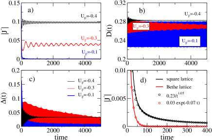
Figure 2: Time dependence of the Gorkov function $J^{-}$ (panels a,d), the double occupancy ${{}D}$ (panel b), and the spectral gap parameter at the chemical potential $\Delta_{\mu}(t)$ (panel c) for a $U$-quench from $U_{i}=-0.5$ to $U_{F}$ with $|U_{F}|<|U_{i}|$. Results in (a-c) are for a half-filled square lattice whereas (d) compares the long time behavior of $J^{-}$ between half-filled Bethe and square lattice for $U_{F}=-0.1$.

III.1 $|U_{F}|<|U_{i}|$ quench

For small quenches (cf. Fig. 2a), similar to the (linearized) BCS dynamics alt06 ; yus06 , the Gorkov function displays a power law, decaying, long-time behavior

$$J^{-}(t)=J^{-}_{\infty}\left[1+\alpha\cos(2\Delta_{\infty}t)/\sqrt{\Delta_{\infty}t}\right]$$ (18)

due to dephasing. volk74 We will refer to the dominant frequency of the Gorkov function at long times as $\Omega_{J}$. It follows from Eq. (18) that

$$\Omega_{J}=2\Delta_{\infty}\equiv 2\langle\Delta_{\mu}(t\to\infty)\rangle_{T}\,,$$ (19)

i.e., the frequency of $J^{-}$ is determined by the long time limit of the spectral gap $\Delta_{\infty}$ at the chemical potential.

Panel (b) of Fig. 2 displays the dynamics of the double occupancy. Because the frequency is much larger than for the Gorkov function, the main oscillation is not resolved and only the envelope is visible as the boundary of the colored regions. We will call the dominant frequency of the double occupancy $\Omega_{U}$. For the cases in which the Gorkov function oscillates and remains finite at long times (black and red), the dynamics resembles two coupled oscillators with a fast frequency $\Omega_{U}$ and a slow frequency $\Omega_{J}$. Indeed, the slow frequency of the Gorkov function $\Omega_{J}$ is clearly visible in the envelop of the double occupancy evolution which shows that $J^{-}$ and ${{}D}$ are significantly coupled. On the other hand, since the natural dynamics of $J^{-}(t)$ is much slower it does not respond to the fast oscillation of ${{}D}(t)$ and therefore the fast oscillations are hardly visible in Fig. 2a. Notice also that the relaxation of ${{}D}(t)$ and $J^{-}(t)$ occurs on the same time scale.

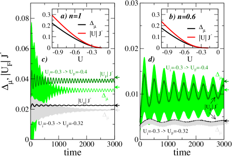
Figure 3: Dynamics of the spectral gap $\Delta_{\mu}$ and the Gorkov function $J^{-}$ near the weak coupling regime. As a reference, the inset panels (a,b) compare the equilibrium spectral gap $\Delta_{\mu}$ (black) with the equilibrium Gorkov function scaled by $|U|$ (red) for densities $n=1$ (a) and $n=0.6$ (b). Panels (c,d): Time dependence of $\Delta_{\mu}$ (light green, grey) and $|U|J^{-}$ (dark green, black) for a $U$-quench from $U_{i}=-0.3$ to $U_{F}=-0.4$ and $U_{F}=-0.32$ for densities $n=1$ (c) and $n=0.6$ (b). Results are for a two-dimensional square lattice. Arrows at the right axis mark the corresponding equilibrium values for $U=U_{F}$.

In case of $J^{-}(t\to\infty)=0$ (blue) one recovers the situation discussed in Refs. fabschi1, ; fabschi2, where the double occupancy oscillates between the two extrema ${{}D}_{-}$ and ${{}D}_{+}$ (upper and lower bounds of the blue curve in (b)).

Panel (d) of Fig. 2 shows the initial stages of the vanishing of $J^{-}$. For some critical value of $|U_{F}|<|U_{i}|$ the Gorkov function dynamically vanishes and in this limit the decay from an initial $J_{i}^{-}$ is described by the general asymptotic behavior derived in Ref. yus06,

$$\frac{J^{-}(t)}{J^{-}_{i}}=A(t)e^{-2\alpha J^{-}_{i}t}+B(t)e^{-2J^{-}_{i}t}$$ (20)

where $A(t)$ and $B(t)$ are decaying power laws $\sim 1/t^{\nu}$ with $1/2\leq\nu\leq 2$ and $0\leq\alpha\leq 1$. As shown in the figure, the decay in the 2D system follows a $1/t$ law whereas for the Bethe lattice it is exponential, both behaviors being particular cases of Eq. (20).

In general in the TDGA and for moderate to large $U_{i}$, the dynamics of the spectral gap (cf. Fig. 2c) is determined by both, the fast double occupancy oscillations at frequency $\Omega_{U}$ (which are not resolved in the figure), and the slower oscillations of the Gorkov function at frequency $\Omega_{J}$, which are revealed in the envelope of $\Delta(t)$.

III.2 $|U_{F}|>|U_{i}|$ quench

III.2.1 Weak and moderate coupling

One way to characterize the weak coupling (BCS) limit of the dynamics is by comparing the spectral gap $\Delta_{\mu}$ with the product of the interaction and the Gorkov function $J^{-}$. For small values of the interaction and small interaction quenches one should recover the BCS dynamics where the two quantities are related by $\Delta_{\mu}=|U|J^{-}$. We first check the range of validity of this expression at equilibrium in the inset panels of Fig. 3a,b, where both sides of the equation are shown as a function of the interaction. We see that in this case this relation holds when both quantities become exponentially small i.e. for small attractive interaction.

In order to study the crossover in the non-equilibrium case we show in Fig. 3c,d the dynamics of $\Delta_{\mu}$ and $|U|J^{-}$ for interaction quenches from $U_{i}=-0.3$ to $U_{F}=-0.4$ and $U_{F}=-0.32$. It can be seen that dynamically at short times the difference between $\Delta_{\mu}$ and $|U|J^{-}$ becomes important, even in a regime where the equilibrium computation shows small or moderate differences. Indeed, $\Delta_{\mu}$ shows again the fast dynamics due to the double occupancy fluctuations which are absent in $|U|J^{-}$. On the other hand, the asymptotic slow dynamics is similar in both quantities.

At half-filling (Fig. 3c) the $\Delta_{\mu}$ fast dynamics tends to get damped at large times, so a single frequency dominates the dynamics similar to the case of $|U|J^{-}$. Away from half-filling (Fig. 3d) this is not anymore true.

Comparing large ($U_{F}=-0.4$) and small ($U_{F}=-0.32$) quenches in Fig. 3 we see that the transient phase extends longer in time for smaller quenches but the associated oscillations of the gap decrease in amplitude with a concomitant decrease in the difference between $\Delta_{\mu}$ and $|U|J^{-}$. Away from half-filling the coupling of the gap to the double occupancy oscillations is significantly enhanced and the associated fast oscillations in $\Delta_{\mu}$ appear with a much larger decay time (not shown, we find $t\approx 10000$ for $U_{i}=-0.3$, $U_{F}=-0.4$, and $n=0.6$). However, similar to the half-filled case the crossover to the BCS dynamics occurs via a decrease of the width of these fast oscillations so that the envelope of $\Delta_{\mu}$ approaches $|U|J^{-}$ in the limit of small interaction quenches (and small $U_{i}$).

In BCS the Larmor precession frequency of pseudospins (corresponding to the phase velocity of the momentum resolved Gorkov function $J^{-}_{k}$) is determined by the $z$ component of the pseudomagnetic field through a Bloch equation as in Eq. (15).yus06 ; bara06 Analogously, here we find that in the regime of Fig. 3 the phase velocity is found to obey $\omega_{p}=2(q_{\parallel}\varepsilon_{k}-\mu)$ [cf. Eq. (16)].

In general for $U_{F}<U_{i}$ and small or moderate interactions the long-time average values of the Gorkov function is slightly below but close to the equilibrium value as in the BCS case. This is shown in panels b and d of Figs. 4 and 5 where the red dots correspond to the $U_{i}$ values. Also the long-time average of the double occupancy and the regular kinetic energy, $T_{0}$, are close to the equilibrium vales (panels a and d). Notice that the kinetic energy has also an anomalous part (insets of Fig. 7) which however is much smaller in magnitude.

Superconducting correlations weakly influence on the characteristic frequency of the double occupancy oscillations $\Omega_{U}$ in this regime. In the half-filled system a linear response analysis bueni13 yields $\Omega_{U}=4|\varepsilon_{0}|\sqrt{q_{0}}$ where $\varepsilon_{0}$ denotes the energy (per site) of the non-interacting system and $q_{0}$ is the (equilibrium) Gutzwiller renormalization factor. Fig. 6a (star symbol) reveals the reasonable agreement of this estimate with the result of the full calculation (triangles) for small quenches.

III.2.2 Strong coupling

For large quenches $|U_{F}|/|U_{i}|\gg 1$ the BCS dynamics crosses over to a synchronized regime bara04 ; bara06 characterized by phase locked Cooper pair states and an order parameter dynamics which oscillates nonharmonically between two extrema $\Delta_{-}$ and $\Delta_{+}$. Remarkably, even in this regime the main frequency of the order parameter in the pure BCS dynamics is determined by the average spectral gap, i.e. it obeys Eq. (19). Although the proof is simple, we are not aware of it in the BCS literature so we explicitly show it in Appendix B. The validity of the BCS dynamics requires that $|U_{F}|,|U_{i}|\ll 1$. The TDGA approximation allows to relax that restriction and explore the intermediate and large coupling regime.

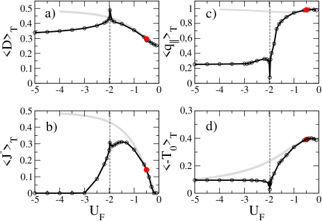
Figure 4: Long-time averages of double occupancy (a), Gorkov function (b), Gutzwiller renormalization factor (c), regular kinetic energy, $T_{0}$ (d) for a quench from $U_{i}=-0.5$ to $U_{F}$ for a half-filled square lattice. The red dots correspond to the equilibrium values at $U_{i}$ and the vertical dotted line indicates the dynamical phase transition at $U_{c}$. The gray lines show the equilibrium value for $U=U_{F}$.

For large quenches with $|U_{F}|>|U_{i}|$ and away from weak coupling the Gutzwiller dynamics is quite different from the BCS dynamics with the former approaching a dynamical phase transition at $U_{c}$. fabschi1 ; fabschi2 ; sandri13 ; mazza17 This is characterized by the dynamics of the phase $\eta$ which changes from oscillating around zero to a precession around the unit circle. Figure 1 compares the density dependence of $U_{c}$ for two initial $U$ values, $U_{i}=-0.5$ and $U_{i}=-1$ with the Brinkman-Rice equilibrium transition. Clearly the typical scale of both transitions is the same.

Exactly at $U_{c}$ the average Gutzwiller renormalization factor $q_{\parallel}$ approaches zero (cf. Appendix C and Fig. 4c), indicative of an insulating state. This is visible as a maximum in the time averaged double occupancy (cf. Figs. 4a, 5a) reaching the value corresponding to full localization ${{}D}=n/2$. At the same time the long-time regular kinetic energy $T_{0}$, (cf. panel (d) in Figs. 4, 5 becomes minimum due to the vanishing of $q_{\parallel}$. Clearly at $U_{c}$ the system reaches full pairing but quasiparticle dephasing effects completely scramble the kinetic energy of the pairs. The spectral gap (Fig. 6) has also a quite interesting behavior. Upon increasing $|U_{F}|$ it first follows a BCS like behavior but then it reaches a maximum and starts to decrease again reaching a minimum at $U_{F}=U_{c}$.

As already mentioned in the previous subsection, the long-time average of the Gorkov function (panel (b) of Figs. 4, 5) initially increases with $|U_{F}|$ and stays slightly below the equilibrium value for $U\equiv U_{F}$ (grey line). At $U_{c}$ the Gorkov function reaches a local maximum. This may appear paradoxical as it implies that the underling BCS state still has a well defined phase and pairing amplitude. In reality the pairs are fully localized so notwithstanding the phase is well defined, this state is extremely fragile i.e., the cost to scramble it is very low. More precisely, we will see that the phase stiffness $\rho_{s}$ tends to vanish. In fact, within standard time-dependent BCS theory the non-equilibrium superfluid stiffness would be equivalent to the average kinetic energy along the direction of the applied vector potential. Therefore the vanishing of $\langle T_{0}\rangle_{T}$ at $U_{c}$ can be considered as a “first indicator” for the vanishing of $\rho_{s}$ at $U_{c}$. However, due to the momentum dependent SC gap the evaluation of $\rho_{s}$ is more subtle in the TDGA and will be analyzed in Sec. VI.

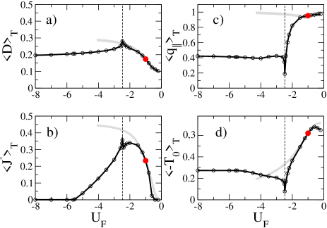
Figure 5: Same as Fig. 4 but for concentration $n=0.6$.

For larger values of $|U_{F}|$ the Gorkov function diminishes and finally vanishes. This suppression of the Gorkov function for large quenches is opposite to what is obtained within the time-dependent BCS approach but agrees with non-equilibrium studies within DMFT werner12 in the context of quenched antiferromagnetism. For the half-filled system this vanishing of the Gorkov function implies the vanishing of local superconducting correlations. However, isotropic superconducting s-wave correlations still persist in this regime as can be seen from the inset to Fig. 6 where we report the long-time average of anomalous kinetic energy correlations $T_{1}$, which contribute to the total energy in the TDGA, cf. Eq. (3). For our two-dimensional system with $\varepsilon_{k}=-2t[\cos(k_{x})+\cos(k_{y})]$, Fourier transformation of Eq.(4) yields a contribution to the energy which only depends on a symmetric combination of SC correlations between nearest neighbors, i.e. extended s-wave symmetry, while the bare (i.e. local) s-wave correlations vanish in the regime of large $U_{F}$ at half-filling. Moving slightly away from half-filling (dashed line in the inset to Fig. 6) the intersite SC correlations vanish together with the Gorkov function. In Sec. V we will analyze this in more detail and show how the double occupancy fluctuations drive the fermions and with increasing strength suppress the average Gorkov function.

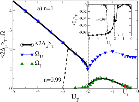
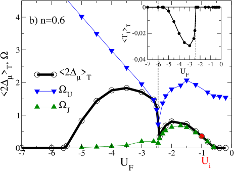
Figure 6: Long-time averages of the spectral gap (black, circles) compared to the main frequencies $\Omega_{U}$ (triangles down, blue) and $\Omega_{J}$ (triangles up, green) in the dynamics for : (a) quench from $U_{i}=-0.5$ and $n=1$, (b) and $U_{i}=-1$ and $n=0.6$. The horizontal axis is the final $U_{F}$ while the red dots indicate $U_{i}$. The dashed line in the inset of panel (a) shows $T_{1}$ for $n=0.99$. The dashed line in the main panel shows the average of the spectral gap for $n=0.99$. The insets reports the long-time average of the anomalous kinetic energy $T_{1}$ (full line), cf. Eq. (3). The vertical dotted line indicates the dynamical phase transition at $U_{c}$. In panel (a) we also show results for $n=0.99$ (dashed line) and the star symbol indicates the value of $\Omega_{U}$ from linear response bueni13 in the normal system.

We now come back to the problem of the relation between $2\Delta(t)$ and $J^{-}$ analyzed in Sec. III.2.1 but now in the strong coupling regime with $|U_{F}|>|U_{c}|$. It is apparent from Fig. 7a,c that as in the previous cases, the dynamics of $2\Delta(t)$ is determined by the fast double occupancy oscillations which are not resolved on the scale of the plot and which give rise to the filled finite width in the time evolution. For the half-filled case (panel a) the average gap increases with $|U_{F}|$ (roughly $2\Delta\sim|U_{F}|$) while the amplitude of the oscillation decreases.

Figure 6(a) compares the characteristic frequencies of the dynamics $\Omega_{U}$ (double occupancy, blue triangles) and $\Omega_{J}$ (Gorkov function, green triangles). Upon increasing $|U_{F}|$, starting from $|U_{i}|$, $\Omega_{J}$ has a dome shape, somehow similar to the Gorkov function $\langle J^{-}\rangle_{T}$ [Fig. 4(b)], until both quantities vanish at $U_{F}\approx-3$. Instead, $\Omega_{U}$ remains high and of the order of the bandwidth until for $|U_{F}|>|U_{c}|$ it increases linearly with $|U_{F}|$. In the same figure we also show the long time average $\langle 2\Delta\rangle_{T}$ (black lines and circles). For $|U_{F}|<|U_{c}|$, $\langle 2\Delta\rangle_{T}$ follows $\Omega_{J}$ (similar to the BCS case) but then it jumps abruptly at $U_{c}$ to $\Omega_{U}$. Notice that $\langle 2\Delta\rangle_{T}=\Omega_{U}$ holds even in the regime where $\langle J^{-}\rangle_{T}=0$. Thus for $|U_{F}|\gtrsim 3$ the half-filled system is characterized by finite intersite but vanishing local SC correlations and the persistence of an average spectral gap which is of the same energy scale than the local on-site attraction.

For slight deviations from half-filling and $|U_{F}|\gg|U_{i}|$ (cf. dashed line in Fig. 6) the time evolution of the spectral gap starts from an initial value $\Delta_{\mu}\sim|U_{F}|$ but then relaxes with a $1\sqrt{t}$ behavior to zero ($n=0.99$ in Fig. 7).

The dynamics of the gap and the Gorkov function for a smaller concentration $n=0.6$ and $|U_{F}|>|U_{i}|$ is shown in panels (c,d) of Fig. 7 and the corresponding long-time averages in Fig. 5, 6b. Similar to the half-filled case the frequency $\Omega_{J}$ is related to the spectral gap up to the dynamical phase transition. For $|U_{F}|>|U_{c}|$ the spectral gap initially follows $\Omega_{U}$ but then goes through a maximum and vanishes together with the average Gorkov function, the intersite SC correlations (inset), and $\Omega_{J}$.

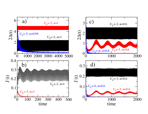
Figure 7: Dynamics of the spectral gap $\Delta(t)$ (panels a,c) and the Gorkov function $J^{-}(t)$ (panels b,d) in the regime $|U_{F}|>|U_{i}|$ for $U_{i}=-0.5$, $n=1$ (panels a,b) and $U_{i}=-1$, $n=0.6$ (panels c,d).

IV DOS

In order to analyze the out-of equilibrium spectral properties we evaluate the density of states (DOS) obtained from the average

$$\langle\rho(\omega)\rangle_{T} = \frac{1}{T}\int_{t_{0}}^{t_{0}+T}\!\!\!dt\rho(\omega,t)$$ (21)

$$\rho(\omega,t) = Im\frac{1}{N\pi}\sum_{k}\frac{\omega+H_{11}^{GA}(k)}{(\omega-i\eta)^{2}-(H_{11}^{GA}(k,t))^{2}-|\Delta_{k}(t)|^{2}}$$

where $t_{0}$ denotes a time scale after the initial transient dynamics and $T$ is ’sufficiently longer’ than the characteristic periodicities of the system. The elements of the Gutzwiller Hamiltonian $H^{GA}$ are defined in appendix A.

Figure 8: Long-time averages of the DOS evaluated from Eq. (21) for $n=1$ (a,b) and $n=0.6$ (c,d) and different quenches as indicated in the panels. Also shown are the characteristic frequencies (where sizeable) $\Omega_{J}$, $\Omega_{U}$, cf. Figs. 4, 5. The yellow shaded areas indicate the variation of the spectral gap in the time-evolution (cf. Fig. 7). Parameters for the evaluation of $\langle\rho(\omega)\rangle_{T}$, cf. Eq. (21): $t_{0}=500$, $T=100$, $\eta=5\cdot 10^{-3}$.

Fig. 8 reports the DOS for concentrations $n=1$ and $n=0.6$ in case of different quenches $|U_{F}|>|U_{i}|$. Clearly the oscillation amplitude of $\Delta_{k}(t)$ has a large impact on the low energy structure of $\langle\rho(\omega)\rangle_{T}$. For example, at half-filling and a quench $U_{i}=-0.5\to U_{F}=-1.5$ the spectral gap oscillates between $0\lesssim|\Delta(t)|\lesssim 0.5$ (not shown) which gives the impression of a ’d-wave’-shaped gap in the temporal average. Neither $\Omega_{J}=\langle 2\Delta\rangle_{T}$ nor $\Omega_{U}$ are apparent as peculiar feature in the averaged DOS. On the other, in case $U_{i}=-0.5\to U_{F}=-2.5$ (panel b) the frequency $\Omega_{U}=\langle 2\Delta\rangle_{T}$ fits to the transition between two peaky structures in the DOS. For even larger values of $|U_{F}|$ this feature is washed out (not shown). Note that for the parameters of panel (b) also $\Omega_{J}\approx 0.024$ is finite but quite small.

For the doped system $n=0.6$ and a quench $U_{i}=-1.0\to U_{F}=-2.0$ it is the excitation energy $\Omega_{J}$ which now fits to the transition between two peaky structures in the DOS (panel c). For larger quenches $\Omega_{J}$ decreases and does not appear any more in the DOS (panel d).

V Frequency mixing and Self-sustained Rabi oscillations

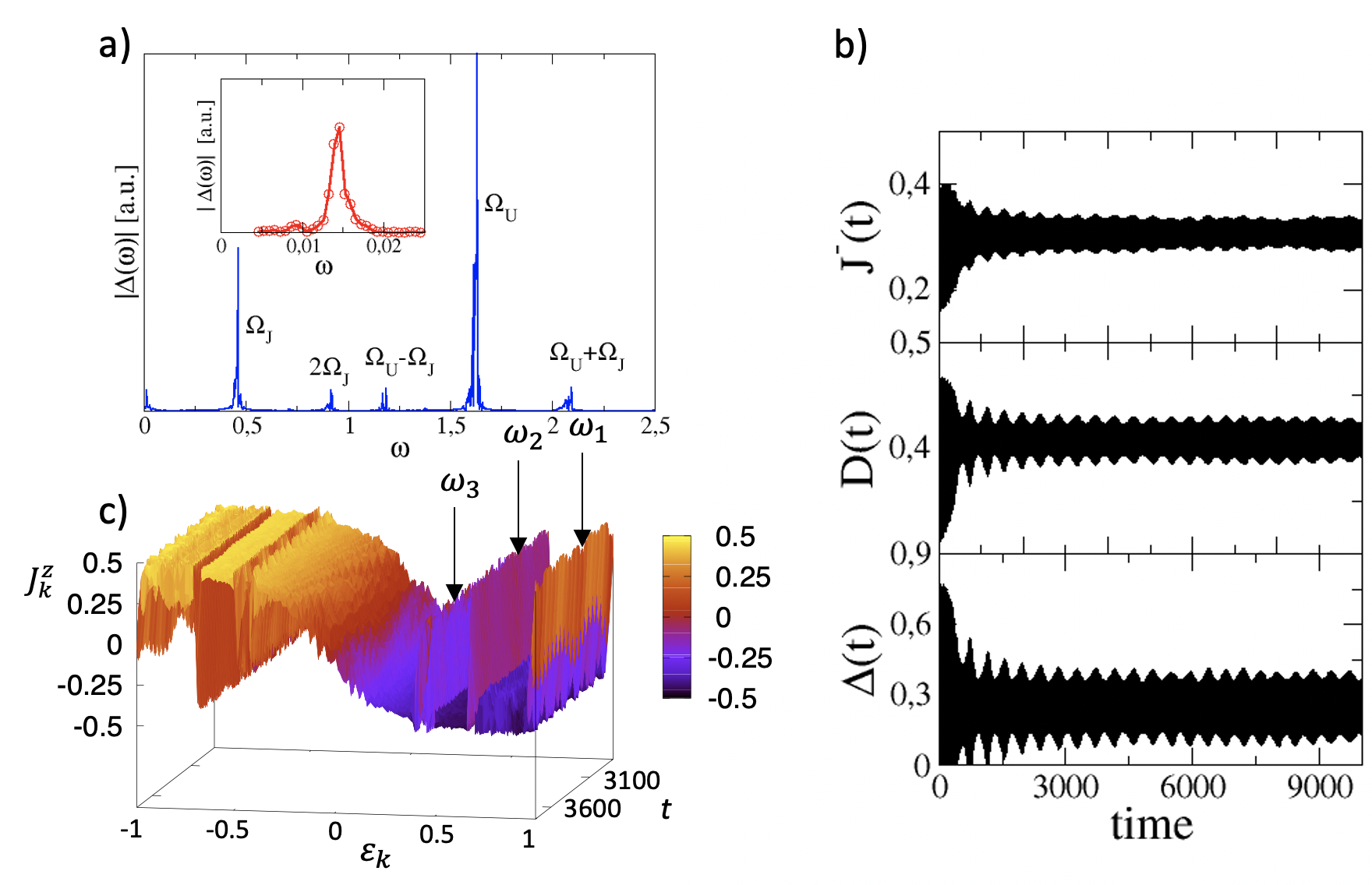
Figure 9: a) Fourier spectrum of $\Delta(\omega)$. The inset details the low energy part with the Rabi excitation. Quench $U_{i}=-0.5\to U_{F}=-1.6$ in the half-filled 2D system. b) Energy and time dependence of the pseudospin $J_{k}^{z}$ showing population inversion at frequencies $\omega_{1,2,3}$. c) From top to bottom: Gorkov function, double occupancy, and spectral gap.

In BCS the spectral gap after a quench oscillates with its natural frequency $\Omega_{J}$. As it is clear from Figs. 2,3,7 the Gutzwiller dynamics is more complex. Besides the frequency $\Omega_{J}$ the spectral gap responds to the fast oscillations of the double occupancy with frequency $\Omega_{U}$. Figure 9 shows the Fourier transform of the spectral gap. We see indeed that $\Omega_{J}$ and $\Omega_{U}$ emerge as the prevailing frequencies, but due to the intrinsic non-linearities of the dynamics other frequencies emerge.

From the equations of motion, we notice that the double occupancy oscillations are seen by the pseudospin degrees of freedom as ’external’ drives. In fact, the modulation of the bandwidth via $q_{\parallel}(t)$ [cf. Eq. (16)] adds a time dependence to the effective magnetic field along the z-direction, $b_{k}^{z}=q_{\parallel}(t)\varepsilon_{k}$ which we write as $b_{k}^{z}=b_{k}^{z,0}+\delta b_{k}^{z}(t)$. Here $b_{k}^{z,0}=\langle q_{\parallel}(t)\rangle_{T}\varepsilon_{k}$ is determined by the temporal average of the renormalization factor and we approximate the time dependent part as $\delta b_{k}^{z}(t)\approx\gamma\varepsilon_{k}\cos(\Omega_{D})$ where $\Omega_{D}$ is the frequency of the drive. In linear response, the spectral gap responds to fluctuations of the double occupancy, $\delta D$ at the frequency of the driving according to,

$$\delta\Delta_{\mu}(t)=\chi_{\Delta n}\delta b_{k}^{z}(t).$$ (22)

where $\chi_{\Delta n}$ is a gap-charge susceptibility (see Ref. collado18, for an analogous treatment in the BCS problem). In addition, there is an explicit dependence of $\Delta_{\mu}$ on $D$ through equations Eqs. (A), (28)-(A). So overall we can write,

$$\delta\Delta_{\mu}(t)=\left(\chi_{\Delta n}\frac{\partial b_{k}^{z}}{\partial D}+\frac{\partial\Delta_{\mu}}{\partial D}\right)\delta D(t).$$ (23)

This explains the appearance of the $\Omega_{U}$ peak in Fig. 9(a). Extending the expansion to second order in the $\delta D(t)$ and $\delta J^{\pm}(t)$ fluctuations explains the $2\Omega_{J}$ and the $\Omega_{U}\pm\Omega_{J}$ peaks. In fact, Raman like matrix elements $\partial\chi_{\Delta n}/{\partial J^{\pm}}$ produce Stokes and anti-Stokes responses at $\Omega_{U}\pm\Omega_{J}$ and the second harmonic frequency $2\Omega_{J}$ is generated from $\delta J^{+}(t)\delta J^{-}(t)$ terms which are already present in $\delta b_{k}^{z}(t)$ through Eq. (28).

Besides these linear and Raman like processes another slower characteristic frequency appears when one examines the dynamics in very long time windows. For example, for quenches $|U_{i}|<|U_{F}|<|U_{c}|$ in the regime where $\langle J^{-}\rangle_{T}$ and $\Omega_{J}$ are maximum ($U_{F}\sim-1.6$ in Fig. 4) one observes very slow oscillations in the envelope of all dynamical quantities as shown in Fig. 9b for the half-filled system and a quench $U_{i}=-0.5\to U_{F}=-1.6$. This new frequency is not directly related to the previous ones. Indeed, the Fourier transform of this oscillation yields $\Omega_{slow}\approx 0.014$ whereas the frequencies of Gorkov function and double occupancy are $\Omega_{J}=0.46$, $\Omega_{U}=1.63$, see Fig. 9c. The slow frequency seems to decrease upon approaching $U_{c}$.

In order to shed some light on this excitation we show in Fig. 9b the pseudospin dynamics of $J_{k}^{z}$ as a function of energy. One observes population inversion at $\omega_{1}\approx 0.98$, $\omega_{2}\approx 0.68$, and $\omega_{3}\approx 0.46$. Such population inversion in the momentum distribution function ($J_{k}^{z}$) is characteristic of collective Rabi oscillations occurring in a superconductor subject to a periodic drive. collado18 ; Collado2020 In the case of a pure BCS dynamics as considered in Ref. collado18 and for a band width drive collective Rabi oscillations are due to states at ’resonant’ energies

$$\varepsilon_{k}\equiv\omega_{r}=\frac{1}{2}\sqrt{\Omega_{D}^{2}-(2\Delta)^{2}}\,.$$ (24)

The corresponding pseudospin will then perform a precession around $b_{k}^{\perp}$, which is the field component of ${\bf b}_{k}(t)$ perpendicular to the static (or time-averaged) field ${\bf b}_{k}^{0}(t)$.collado18 Analogous to magnetic resonance dynamics slichter the precession (’Rabi’) frequency would then be given by

$$\Omega_{R}=\frac{1}{2}b_{k}^{\perp}=\gamma\Delta\sqrt{1-(2\Delta/\Omega_{D})^{2}}\,.$$ (25)

In the present time-dependent Gutzwiller dynamics, drives are generated internally as discussed above. Based on these arguments the frequencies $\omega_{1,2,3}$ at which population inversion is seen in Fig. 9b can be obtained by replacing in Eq. (24) $\Omega_{D}$ by combinations of $\Omega_{U}$ and $\Omega_{J}$ and also including the average band width renormalization $\bar{q}=\langle q_{\parallel}\rangle_{T}$,

$$\omega_{1} = \frac{1}{2\bar{q}}\sqrt{(\Omega_{D}^{(1)})^{2}-(2\Delta)^{2}}\approx 0.98\hskip 5.69046pt\mbox{for}\hskip 5.69046pt\Omega_{D}^{(1)}=\Omega_{U}$$

$$\omega_{2} = \frac{1}{2\bar{q}}\sqrt{(\Omega_{D}^{(2)})^{2}-(2\Delta)^{2}}\approx 0.67\hskip 5.69046pt\mbox{for}\hskip 5.69046pt\Omega_{D}^{(2)}=\Omega_{U}-\Omega_{J}$$

$$\omega_{3} = \frac{1}{2\bar{q}}\sqrt{(\Omega_{D}^{(3)})^{2}-(2\Delta)^{2}}\approx 0.49\hskip 5.69046pt\mbox{for}\hskip 5.69046pt\Omega_{D}^{(3)}=2\Omega_{J}$$

where for the considered quench we have $\bar{q}\approx 0.79$ and $2\Delta\approx 0.49\approx\Omega_{J}$. The combination $\Omega_{U}+\Omega_{J}$ would correspond to a drive outside the available energy spectrum.

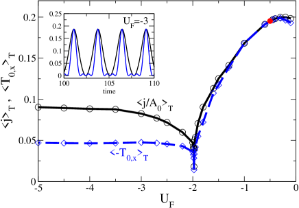
Figure 10: Main panel: Superfluid stiffness $\rho_{s}=j(0)/A_{0}$ (black, solid) compared to the regular kinetic energy (blue, dashed) as a function of the quenched interaction $U_{F}$ for a half-filled square lattice. The red point indicated the equilibrium value $U_{i}$. Inset: Time dependence of both quantities for $U_{F}=-3$.

Based on this knowledge we can now ask the question how these drives are related to the slow Rabi oscillation visible in Fig. 9. Generalizing Eq. (25) to include the bandwidth renormalization and taking $\gamma\approx 0.05$ as obtained from the width of the renormalization factor dynamics $q_{\parallel}(t)$ one obtains

$$\Omega^{(1,2,3)}_{R}=\Delta\frac{\gamma}{\bar{q}}\sqrt{1-(2\Delta/\Omega^{(1,2,3)}_{D})^{2}}\approx 0.015,0.014,0.013\,.$$

Inspection of the low energy Fourier transform of $\Delta(\omega)$ in Fig. 9 reveals a broad excitation centered at $\omega\approx 0.014$ which supports the consistency of our analysis.

VI Optical conductivity

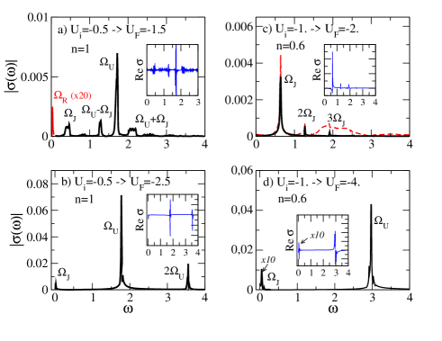
Figure 11: Optical conductivity $\sigma(\omega,t_{1}=50)$ for the same parameters than in Fig. 8. Main panels show the magnitude $|\sigma(\omega,t_{1})|$ whereas insets report the real part. Panel (c) also reports $|\sigma(\omega,t_{1})|$ for $t_{1}=0$ (red dashed) which contains the $\Omega_{U}$ excitations in the transient regime. In panel (a) the Fourier transform has been performed for times up to $t_{max}=2500$ whereas in panels (b-d) $t_{max}=500$.

We finally analyze how the characteristic frequencies, discussed in the previous section, are visible in the optical conductivity. In the non-equilibrium state we evaluate this quantity from the current response

$$j(t)=\int_{t_{0}}^{t_{0}+T}dt^{\prime}\sigma(t,t^{\prime})E(t^{\prime})$$ (26)

to a delta-like electric field $E(t^{\prime})=A_{0}\delta(t^{\prime}-t_{1})$ which is applied within the interval $t_{0}<t_{1}<t_{0}+T$ in which the current is measured. Then the optical conductivity is obtained from the Fourier transformed of Eq. (26) as tohyama

$$j(\omega)=A_{0}e^{i\omega t_{1}}\sigma(\omega,t_{1})\,.$$ (27)

Within our model the delta-shaped electric field is coupled to the system by a step-like vector potential $A(t)=A_{0}\Theta(t-t_{1})$ via the standard Peierls substitution and the current is evaluated from $j(t)=\delta E^{GA}/\delta A$. Then the Fourier transform of $j(t)$ is performed for times $t_{1}\lesssim t\lesssim t_{1}+t_{max}$.

The Peierls substitution for an applied vector potential, say along the $x$-direction, induces a shift of momentum $k_{x}\rightarrow k_{x}+A_{x}$. Within standard time-dependent BCS theory and in the linear response limit this leads to a purely time-dependent diamagnetic current which therefore is equivalent to the time-dependent kinetic energy. The superfluid stiffness $\rho_{s}$, defined as the $\omega=0$ component of this current comment is then just the time averaged kinetic energy. In the TDGA the Peierls substitution also influences on the pairing term $\sim q_{\perp}\varepsilon_{k}$ [cf. Eqs. (3,4) and appendix A] which generates an additional pairing component to the current, which is significant in particular at large quenches $U_{F}$ and close to half-filling as can be seen from the inset to Fig. 10. The main panel of Fig. 10 compares $\rho_{s}$ with the regular kinetic energy [cf. Eq. (4)] along $x$ as function of the quenched interaction $U_{F}$. For $U_{F}\approx U_{i}$ both quantities coincide since in this limit the oscillation of the double occupancy phase vanish and therefore also $q_{\perp}\to 0$. Differences occur for large quenches and close to half-filling, in particular for $|U_{F}|>|U_{c}|$ the normal component of the kinetic energy underestimates the stiffness by almost a factor of two for the present parameters.

Fig. 11 shows $\sigma(\omega,t_{1})$ for the same quench situations than analyzed for the DOS, cf. Fig. 8. For a better visualization of the involved frequencies we show in the main panel the magnitude $|\sigma(\omega,t_{1})|$ whereas the insets display the real part $\sigma^{\prime}(\omega,t_{1})$ with $t_{1}=50$. We observe that both frequencies $\Omega_{J}$ and $\Omega_{U}$ are visible in $\sigma(\omega,t_{1})$ except for panel c) where the $\Omega_{U}$ oscillations are already damped for $t<t_{1}=50$ and are only visible as a broad feature if the field is switched on already at $t_{1}=0$ (red dashed). A further feature is the coupling of the order parameter to the double occupancy dynamics, as discussed in the previous section, which is especially apparent in panel (a) of Fig. 11 where $\Omega_{U}$ has two side peaks at $\Omega_{U}\pm\Omega_{J}$ as discussed in the previous section. This coupling is also present in panels (b,d) but hardly visible on the scale of the plot due to the smallness of $\Omega_{J}$. In panel (a) we have performed the Fourier transform up to large times $t_{max}=2500$ which includes several Rabi periodicities. The Rabi oscillation is visible in $\sigma({\omega})$ though the intensity is much smaller than those of the main excitations at $\Omega_{J}$ and $\Omega_{U}$. Finally, it should be noted that for large quenches higher harmonics of $\Omega_{U}$ appear in the conductivity (cf. panel c).

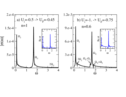
Figure 12: Optical conductivity $\sigma(\omega,t_{1}=50)$ for quench situations $|U_{F}|<|U_{i}|$. Main panels show the magnitude $|\sigma(\omega,t_{1})|$ whereas insets report the real part. The Fourier transform has been performed up to $t_{max}=500$.

Similar features can also be seen in Fig. 12 which reports the optical conductivity now for quench situations $|U_{F}|<|U_{i}|$. In both cases the double occupancy oscillations are modulated by the oscillations of the Gorkov function. For the large quench in panel (b) the corresponding side bands are clearly visible in $\sigma(\omega)$ together with higher harmonics in $\Omega_{J}$ and $\Omega_{U}$.

VII Conclusions

We have analyzed the dynamics of out-of equilibrium superconductivity within the time-dependent Gutzwiller approximation. As shown previously sandri13 ; mazza17 this approach correctly reproduces certain aspects of non-equilibrium DMFT werner12 ; tsuji13 ; balzer15 as the trapping in non-thermal states and the appearance of two energy scales in the transient dynamics.

In particular, DMFT reveals a sharp crossover in the dynamics of the Hubbard model upon quenching the non-interacting system to a finite interaction $U$. eckstein09 In the weak coupling regime, below a critical interaction $U_{c}$, the double occupancy $D(t)$ relaxes to the almost thermalized value whereas for strong coupling $D(t)$ recovers and oscillates with frequency $\sim U$.

The TDGA captures this feature as a ’dynamical generalization’ of the Brinkman-Rice transition br where upon approaching $U_{c}$ the period, in which Gutzwiller renormalization factors tend to zero, logarithmically diverges. fabschi1 ; fabschi2 In the repulsive Hubbard model the Brinkman-Rice transition is only present in the half-filled system but in the attractive model occurs independent of filling.

Two main frequencies, $\Omega_{U}$ and $\Omega_{J}$, determine the dynamical quantities within the TDGA which for small quenches are related to the double occupancy and SC pair correlation dynamics. Here we have shown that the dynamical phase transition at $|U_{c}|$ is also associated with a crossover, where the time-averaged SC gap follows $\Omega_{J}$ for $|U_{F}|<|U_{c}|$ whereas it is bound to $\Omega_{U}$ in a region $|U_{F}|>|U_{c}|$ which depends on the filling. Interestingly, at half-filling the average spectral gap keeps following $\Omega_{U}\sim|U_{F}|$ for increasing quenches $|U_{F}|$, even when the local pair correlations are already suppressed. We have shown that this regime is instead characterized by intersite SC correlations (extended s-wave symmetry) which also influence on the superconducting stiffness. It would be interesting to see whether such crossover from local to extended s-wave superconducting correlations is also obtained in more exact approaches.

The TDGA can be viewed as a driven BCS model where the drive acts on the bandwidth via the time dependence of the Gutzwiller renormalization factors. In an out-of equilibrium situation we have shown that the characteristic drive frequency is not only due to the double occupancy dynamics but can be a linear combination of the basic frequencies $\Omega_{U}$ and $\Omega_{J}$. This yields a consistent explanation for the structure of low energy Rabi oscillations which can be observed in all dynamical quantities in certain parameter regimes where the resonant condition can be fulfilled. Moreover, since for a bandwidth driven BCS model the increase of the drive amplitude results in a suppression of the Gorkov function, it is most likely that the same mechanism is also responsible in the TDGA for the vanishing of $J^{-}$ at large interaction quenches.

The TDGA does not include thermalization mechanisms so that in the long-time limit integrated quantities stay either oscillating or decay due to dephasing, cf. Fig. 7, whereas in an exact treatment one expects damping on a time scale $\tau_{th}$. The open question therefore remains if real systems can be tuned towards a regime where $\tau_{th}$ is significantly larger than the Rabi periodicity which would allow the observation of the latter by non-equilibrium spectroscopic methods.

Appendix A

The renormalization factors in Eq. (3) are given by

$$q_{\parallel} = Q_{+}^{2}+\frac{J_{z}^{2}-J^{+}J^{-}}{J^{2}}Q_{-}^{2}$$ (28)

$$q_{\perp} = 2iQ_{-}\frac{J^{-}}{J}\left[Q_{+}-iQ_{-}\frac{J^{z}}{J}\right]$$ (29)

with

$$Q_{+} = \sqrt{\frac{\frac{1}{2}-{{}D}+J_{z}}{\frac{1}{4}-J^{2}}}\left[\sqrt{{{}D}-J_{z}-J}\right.$$

$$+ \left.\sqrt{{{}D}-J_{z}+J}\cos\eta\right]$$

$$Q_{-} = \sqrt{\frac{\frac{1}{2}-{{}D}+J_{z}}{\frac{1}{4}-J^{2}}}\sqrt{{{}D}-J_{z}+J}\sin\eta\,.$$

Then the matrix elements become

$$H_{11}(k) = q_{\parallel}\varepsilon_{k}-\mu+\frac{U}{2}(1-\frac{J^{z}}{J})$$

$$+ \frac{\partial q_{\parallel}}{\partial J^{z}}\frac{1}{2N}\sum_{k^{\prime}}\varepsilon_{k^{\prime}}\left[R_{11}(k^{\prime})-R_{22}(k^{\prime})+1\right]$$

$$+ \frac{1}{2N}\sum_{k^{\prime}}\varepsilon_{k^{\prime}}\left[\frac{\partial q_{\perp}}{\partial J^{z}}R_{12}({k^{\prime}})+\frac{\partial q^{*}_{\perp}}{\partial J^{z}}R_{21}({k^{\prime}})\right]$$

$$H_{12}(k) = q_{\perp}^{*}\varepsilon_{k}-\frac{U}{2}\frac{J^{+}}{J}$$

$$+ \frac{\partial q_{\parallel}}{\partial J^{-}}\frac{1}{N}\sum_{k^{\prime}}\varepsilon_{k^{\prime}}\left[R_{11}({k^{\prime}})-R_{22}({k^{\prime}})+1\right]$$

$$+ \frac{1}{N}\sum_{k^{\prime}}\varepsilon_{k^{\prime}}\left[\frac{\partial q_{\perp}}{\partial J^{-}}R_{12}({k^{\prime}})+\frac{\partial q^{*}_{\perp}}{\partial J^{-}}R_{21}({k^{\prime}})\right]$$

$$H_{21}(k) = q_{\perp}\varepsilon_{k}-\frac{U}{2}\frac{J^{-}}{J}$$

$$+ \frac{\partial q_{\parallel}}{\partial J^{+}}\frac{1}{N}\sum_{k^{\prime}}\varepsilon_{k^{\prime}}\left[R_{11}({k^{\prime}})-R_{22}({k^{\prime}})+1\right]$$

$$+ \frac{1}{N}\sum_{k^{\prime}}\varepsilon_{k^{\prime}}\left[\frac{\partial q_{\perp}}{\partial J^{+}}R_{12}({k^{\prime}})+\frac{\partial q^{*}_{\perp}}{\partial J^{+}}R_{21}({k^{\prime}})\right]$$

$$H_{22}(k) = H_{11}(k).$$ (34)

The spectral gap in Eq. (17) is defined as $\Delta_{k}=H^{GA}_{12}(k)=\Delta_{\mu}+\Delta_{k}^{\prime}$ with

$$\Delta_{\mu} \equiv \mu\frac{q_{\perp}^{*}}{q_{\parallel}}-\frac{U}{2}\frac{J^{+}}{J}$$

$$+ \frac{\partial q_{\parallel}}{\partial J^{-}}\frac{1}{N}\sum_{k}\varepsilon_{k}\left[R_{11}({k})-R_{22}({k})+1\right]$$

$$+ \frac{1}{N}\sum_{k}\varepsilon_{k}\left[\frac{\partial q_{\perp}}{\partial J^{-}}R_{12}({k})+\frac{\partial q^{*}_{\perp}}{\partial J^{-}}R_{21}({k})\right],$$

$$\Delta_{k}^{\prime} \equiv \frac{q_{\perp}^{*}}{q_{\parallel}}(q_{\parallel}\varepsilon_{k}-\mu).$$ (36)

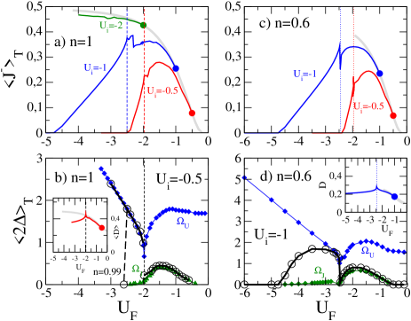
Figure 13: Long-time averages of the Gorkov function (a,c) and spectral gap (b,d) for the Bethe lattice with infinite coordination number and concentrations $n=1$ (a,b) and $n=0.6$ (c,d). Panels (b,d) also report the frequencies $\Omega_{U}$, $\Omega_{J}$ and the insets show the long time average of the double occupancy.

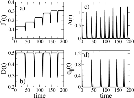
Figure 14: Dynamics of the Gorkov function (a), double occupancy (b), hopping renormalization $q_{\parallel}$ (c) and spectral gap (d) in close vicinity to $U_{c}$. Results are obtained on a Bethe lattice with infinite coordination number and concentration $n=1$.

Appendix B

Consider the synchronized regime where the self-consistent BCS dynamics is governed by the equation bara04

$$\dot{\Delta}^{2}+\left(\Delta^{2}-\Delta_{-}^{2}\right)\left(\Delta^{2}-\Delta_{+}^{2}\right)=0\,.$$ (37)

and shows soliton solutions of the order parameter oscillating between $\Delta_{-}\leq\Delta(t)\leq\Delta_{+}$ . The oscillation period is then determined from

$$T=2\int_{T_{-}}^{T_{+}}\!\!\!dt=\int_{\Delta_{-}}^{\Delta_{+}}\frac{d\Delta}{\dot{\Delta}}\,.$$ (38)

Similarly, the time-averaged order parameter is obtained from

$$\langle\Delta\rangle_{T}=\frac{2}{T}\int_{\Delta_{-}}^{\Delta_{+}}\!\!d\Delta\,\frac{\Delta}{\dot{\Delta}}$$ (39)

so that

$$\langle\Delta\rangle_{T}=\frac{\omega}{\pi}\int_{\Delta_{-}}^{\Delta_{+}}d\Delta\frac{\Delta}{\sqrt{\left(\Delta^{2}-\Delta_{-}^{2}\right)\left(\Delta_{+}^{2}-\Delta^{2}\right)}}=\frac{\omega}{2}$$ (40)

where we have used Eq. (37) and $\omega=2\pi/T$ is the frequency of the oscillation. Thus also in the synchronized regime the main frequency $\omega$ of the BCS dynamics is determined by the time-averaged spectral gap $2\langle\Delta\rangle_{T}$.

Appendix C

Fig. 13 reports the long-time averages of spectral gap (a,c) and Gorkov function (b,d) for a Bethe-lattice with infinite coordination number. No qualitative changes occur with regard to the 2-D case shown in Figs. 4, 5.

The time dependence of Gorkov function $J^{-}(t)$, double occupancy $D(t)$, hopping renormalization $q_{\parallel}(t)$, and spectral gap $\Delta(t)$ close to the dynamical phase transition is shown in Fig. 14. The dynamics in this regime is characterized by a periodic soliton like behavior with long localization time periods where $D(t)$ takes the Brinkman-Rice value ($D=0.5$ for $n=1$) and the hopping renormalization $q_{\parallel}$ vanishes. The time dependence of the phase $\eta(t)$ has a periodicity with twice the frequency of $D(t)$, $J^{-}(t)$, and $q_{\parallel}(t)$ which reflects also in the dynamics of the spectral gap $\Delta(t)$ (panel c).

References

- (1) C. A. Regal, M. Greiner, and D. S. Jin, Phys. Rev. Lett. 92, 040403 (2004).
- (2) M. W. Zwierlein, C. A. Stan, C. H. Schunck, S. M. F. Raupach, A. J. Kerman, and W. Ketterle, Phys. Rev. Lett. 92, 120403 (2004).
- (3) M. Bartenstein, A. Altmeyer, S. Riedl, S. Jochim, C. Chin, J. Hecker Denschlag, and R. Grimm, Phys. Rev. Lett. 92, 203201 (2004).
- (4) C. Chin, R. Grimm, P. Julienne, and E. Tiesinga, Rev. Mod. Phys. 82,1225 (2010).
- (5) A. Behrle, T. Harrison, J. Kombe, K. Gao, M. Linkl, J.-S. Bernier, C. Kollath, and M. Köhl, Nature Physics 2018, https://doi.org/10.1038/s41567-018-0128-6.
- (6) B. Mansart, J. Lorenzana, A. Mann, A. Odeh, M. Scarongella, M. Chergui, and F. Carbone, Proc. Natl. Acad. Sci. 110, 4539 (2013).
- (7) R. Matsunaga, Y. I. Hamada, K. Makise, Y. Uzawa, H. Terai, Z. Wang, and R. Shimano, Phys. Rev. Lett. 111, 1 (2013).
- (8) R. Matsunaga, N. Tsuji, H. Fujita, A. Sugioka, K. Makise, Y. Uzawa, H. Terai, Z. Wang, H. Aoki, and R. Shimano, Science 345, 1145 (2014).
- (9) J. Bünemann and G. Seibold, Phys. Rev. B 96, 245139 (2017).
- (10) H. P. Ojeda Collado, G. Usaj, J. Lorenzana, and C. A. Balseiro, Phys. Rev. B 99, 174509 (2019).
- (11) H. P. Ojeda Collado, G. Usaj, J. Lorenzana, and C. A. Balseiro, Phys. Rev. B 101, 054502 (2020).
- (12) M. Udina, T. Cea, and L. Benfatto, Phys. Rev. B 100, 165131 (2019).
- (13) T. Papenkort, V. M. Axt, and T. Kuhn, Phys. Rev. B 76, 224522 (2007).
- (14) T. Papenkort, T. Kuhn, and V. M. Axt, Phys. Rev. B 78, 132505 (2008).
- (15) H. Krull, D. Manske, G. S. Uhrig, and A. P. Schnyder, Phys. Rev. B 90, 014515 2014).
- (16) H. P. O. Collado, J. Lorenzana, G. Usaj, and C. A. Balseiro, Phys. Rev. B 98, 214519 (2018).
- (17) P. W. Anderson, Phys. Rev. 112, 1900 (1958).
- (18) R. A. Barankov, L. S. Levitov, and B. Z. Spivak, Phys. Rev. Lett. 93, 160401 (2004).
- (19) E. A. Yuzbashyan, B. L. Altshuler, V. B. Kuznetsov, and V. Z. Enolskii, J. Phys. A: Math. Gen. 38, 7831 (2005).
- (20) R. A. Barankov and L. S. Levitov, Phys. Rev. Lett. 96, 230403 (2006).
- (21) E. A. Yuzbashyan, O. Tsyplyatyev, and B. Altshuler, Phys. Rev. Lett. 96, 097005 (2006).
- (22) E. A. Yuzbashyan and M. Dzero, Phys. Rev. Lett. 96, 230404 (2006).
- (23) M. Randeria and E. Taylor, Annu. Rev. Condens. Matter Phys. 5, 209 (2014).
- (24) R. S. Markiewicz, J. Lorenzana, G. Seibold, and A. Bansil, Phys. Rev. B 81, 014509 (2010).
- (25) J Bünemann, M. Capone, J. Lorenzana, and G. Seibold, New Journal of Physics 15, 053050 (2013).
- (26) M. Schiró and M. Fabrizio, Phys. Rev. Lett. 105, 076401 (2010).
- (27) M. Schiró and M. Fabrizio, Phys. Rev. B 83, 165105 (2011).
- (28) G. Seibold and J. Lorenzana, Phys. Rev. Lett. 86, 2605 (2001).
- (29) G. Seibold, F. Becca, and J. Lorenzana, Phys. Rev. B 67, 085108 (2003).
- (30) G. Seibold, F. Becca, P. Rubin, and J. Lorenzana, Phys. Rev. B 69, 155113 (2004).
- (31) G. Seibold, F. Becca, and J. Lorenzana, Phys. Rev. Lett. 100, 016405 (2008); Phys. Rev. B 78, 0451124 (2008).
- (32) S. Ugenti, M. Cini, G. Seibold, J. Lorenzana, E. Perfetto, and G. Stefanucci, Phys. Rev. B 82, 075137 (2010).
- (33) M. Sandri and M. Fabrizio, Phys. Rev. B 88, 165113 (2013).
- (34) G. Mazza, Phys. Rev. B 96, 205110 (2017).
- (35) M. Eckstein, M. Kollar, and P. Werner, Phys. Rev. Lett. 103, 056403 (2009).
- (36) P. Werner, N. Tsuji, and M. Eckstein, Phys. Rev. B 86, 205101 (2012).
- (37) N. Tsuji, M. Eckstein, and P. Werner, Phys. Rev. Lett. 110, 136404 (2013).
- (38) K. Balzer, F. A. Wolf, I. P. McCulloch, P. Werner, and M. Eckstein, Phys. Rev. X 5, 031039 (2015).
- (39) M. Sandri, M. Schiró, and M. Fabrizio, Phys. Rev. B 86, 075122 (2012).
- (40) G. Mazza and M. Fabrizio, Phys. Rev. B 86, 184303 (2012).
- (41) R. Micnas, J. Ranninger, and S. Robaszkiewicz, Rev. Mod. Phys. 62, 113 (1990).
- (42) G. A. Medina, J. Simonin, and M. D. Núñez Regueiro, Phys. Rev. B 43, 6206 (1991).
- (43) J. O. Sofo and C. A. Balseiro, Phys. Rev. B 45, 377 (1992).
- (44) G. Seibold, F. Becca, and J. Lorenzana Phys. Rev. Lett. 100, 016405 (2008).
- (45) G. Seibold, F. Becca, and J. Lorenzana, Phys. Rev. B 78, 045114 (2008).
- (46) W. F. Brinkman and T. M. Rice, Phys. Rev. B 2, 4302 (1970).
- (47) A. F. Volkov and Sh. M. Kogan, Zh. Eksp. Teor. Fiz. 65, 2038 (1973) [Sov- Phys. JETP 38, 1018 (1974].
- (48) C. P. Slichter, Principles of Magnetic Resonance, Springer Series in Solid-State Sciences Vol. 1 (Springer, Berlin, 1990), p. 655.
- (49) C. Shao, T. Tohyama, H.-G. Luo, and H. Lu, Phys. Rev. B 93, 195144 (2016).
- (50) More precisely the limit has to be taken before the limit for a momentum and frequency dependent vector potential .