Game on Random Environment, Mean-field Langevin System and Neural Networks

Abstract

In this paper we study a type of games regularized by the relative entropy, where the players’ strategies are coupled through a random environment variable. Besides the existence and the uniqueness of equilibria of such games, we prove that the marginal laws of the corresponding mean-field Langevin systems can converge towards the games’ equilibria in different settings. As applications, the dynamic games can be treated as games on a random environment when one treats the time horizon as the environment. In practice, our results can be applied to analysing the stochastic gradient descent algorithm for deep neural networks in the context of supervised learning as well as for the generative adversarial networks.

60H30, 37M25, 91A40

1 Introduction

The approximation of the equilibria is at the heart of the game theory. The classic literature introduces a natural relation connecting the equilibria of the games and the optima of the sequential decision problems. This leads to a fruitful research on the topics such as approachability, regret and calibration, see the survey by V. Perchet [26] and the books by N. Cesa-Bianchi and G. Lugosi [3] and by D. Fudenberg and D. K. Levine [12]. In particular, the gradient-based strategy often plays a crucial rule in approximating the equilibria. In the present paper we study the analog to the gradient-based strategy in the continuous-time setting, namely, we aim at approximating the equilibria of games using the diffusion processes encoded with the gradients of potential functions.

Consider a game with $n$ players. The mixed Nash equilibrium is defined to be a collection of probability measures $(\nu^{*,i})_{i=1,\cdots,n}$ such that

(1) $$\nu^{*,i}\in\operatorname*{\arg\!\min}_{\nu^{i}}\int f^{i}(x^{1},\cdots,x^{n})\nu^{i}(dx^{i})\prod_{j\neq i}\nu^{*,j}(dx^{j}),$$

which means that each player can no longer improve his performance by making a unilateral change of strategy. Note that in this classical setting, the potential function of each player

$$\nu^{i}\mapsto F^{i}\big{(}\nu^{i},(\nu^{j})_{j\neq i}\big{)}:=\int f^{i}(x^{1},\cdots,x^{n})\nu^{i}(dx^{i})\prod_{j\neq i}\nu^{j}(dx^{j})$$

is linear. In this paper we shall allow the potential function to be nonlinear in view of the applications, in particular, to the neural networks (see Section 4). As another generalization to the classic theory, we consider games on a random environment. Introduce a space of environment $\mathbb{Y}$ and fix a probability measure ${\mathsf{m}}$ on it. We urge each player to choose a strategy among the probability measures $\nu^{i}$ on the product space $\mathbb{R}^{n^{i}}\times\mathbb{Y}$ such that the marginal law of $\nu^{i}$ on $\mathbb{Y}$, $\nu^{i}_{Y}$, matches the fixed distribution ${\mathsf{m}}$. Typically, in our framework we consider the game of which the Nash equilibrium is a collection of probability measures $(\nu^{*,i})_{i=1,\cdots,n}$ on the product spaces such that

(2) $$\nu^{*,i}\in\operatorname*{\arg\!\min}_{\nu^{i}:\nu^{i}_{Y}={\mathsf{m}}}\int f^{i}(x^{1},\cdots,x^{n},{\mathsf{y}})\nu^{i}(dx^{i}|{\mathsf{y}})\prod_{j\neq i}\nu^{*,j}(dx^{j}|{\mathsf{y}}){\mathsf{m}}(d{\mathsf{y}})+\frac{\sigma^{2}}{2}H(\nu^{i}|{\rm Leb}\times{\mathsf{m}}),$$

where $\nu(\cdot|{\mathsf{y}})$ denotes the conditional probability given ${\mathsf{y}}$, and we add the relative entropy $H$ as a regularizer. In contrast to the conventional definition of the Nash equilibrium Eq. 1, where the players’ strategies are uncorrelated, in our setting the strategies of the players are allowed to be coupled through the environment. Moreover, the general framework of the present paper goes beyond the particular game Eq. 2, by allowing the cost function to be nonlinear in $(\nu^{i})_{i=1,\cdots,n}$. As an application, we observe (Section 2.2) that relaxed dynamic games can be viewed as games on random environment, where the environment $\mathbb{Y}$ is the time horizon.

One of our main contributions is the first order condition of the optimization on the probability space given a marginal constraint (Theorem 3.1), which naturally provides a necessary condition for being a Nash equilibrium of a game on random environment (Corollary 3.3). This result is a generalization to the first order condition in Proposition 2.4 in [16] for the optimization on the probability space without marginal constraint. The key ingredient for this analysis is the linear functional derivative $\frac{\delta F}{\delta\nu}$, first introduced for the variational calculus and recently popularized by the study on the mean-field games, see e.g. Cardaliaguet et al. [1], Delarue et al. [7, 8], Chassagneux et al. [4]. Roughly speaking, we prove that

(3) $$\mbox{if $\nu^{*}\in\operatorname*{\arg\!\min}_{\nu:\nu_{Y}={\mathsf{m}}}F(\nu)+\frac{\sigma^{2}}{2}H(\nu|{\rm Leb}\times{\mathsf{m}})$,}\\ \mbox{then $\nabla_{x}\frac{\delta F}{\delta\nu}(\nu^{*},x,{\mathsf{y}})+\frac{\sigma^{2}}{2}\nabla_{x}\ln\nu^{*}(x|{\mathsf{y}})=0$, for all $x$, ${\mathsf{m}}$-a.s. ${\mathsf{y}}$. }$$

Besides the first order condition for the Nash equilibrium, we also provide sufficient conditions on the linear functional derivative so that the game on a random environment admits a (unique) equilibrium.

The first order equation in Eq. 3 clearly links the minimizer $\nu^{*}$ (or the Nash equilibrium in the context of games) to the invariant measure of a system of diffusion processes, see Eq. 5 below. Since the dynamics of the diffusion processes depends on their marginal distributions (in other word, McKean-Vlasov diffusion, see [24, 27]) and involves the gradients of the potential functions, we name the system mean-field Langevin (MFL) system. Further, we study the different settings where the marginal laws of the MFL system converge to the unique invariant measure, which, due to the first order condition, must coincide with the Nash equilibrium of the game on random environment. In the case with small dependence on the marginal laws, we prove the exponential ergodicity of the MFL system, using the reflection coupling (see [10, 11]). In the case of one-player game (in other word, optimization), once the potential function is convex, we use an argument, similar to that in [16, 15], based on the Lasalle’s invariant principle to prove the (non-exponential) ergodicity of the MFL system under mild conditions on the coefficients.

In view of applications, our result can be used to justify the applicability of the gradient descent algorithm for training (deep) neural networks. As mentioned in [17, 23, 22, 16, 15], the supervised learning with (deep) neural networks can be viewed as a minimization problem (or optimal control problem in the context of deep learning) on the space of probability measures, and the gradient descent algorithm is approximately a discretization of the corresponding mean-field Langevin dynamics. The present paper provides a more general framework for such studies. In particular, it is remarkable that in Section 4 we provide a theoretically convergent numerical scheme for the generative adversarial networks (GAN) as well as a way to characterize the training error.

The rest of the paper is organized as follows. In Section 2 we introduce the definitions of a game on a random environment and the corresponding MFL system. In Section 3 the main theorems of the paper are stated without proofs. In Section 4 we present the applications to the dynamic games and the GAN. Finally in Section 5 we present the proofs of the main theorems.

2 Notation and definitions

2.1 Preliminary

Denote by $\mathbb{Y}$ the space of environment, and assume $\mathbb{Y}$ to be Polish. Throughout the paper, we fix a probability measure ${\mathsf{m}}$ on $\mathbb{Y}$. Define the product space $\bar{\mathbb{R}}^{d}:=\mathbb{R}^{d}\times\mathbb{Y}$ for $d\in\mathbb{N}$. In this paper we consider a game in which the players choose strategies among $\Pi:=\{\bar{\pi}\in{\cal P}_{p}(\bar{\mathbb{R}}^{d}):\bar{\pi}(\mathbb{R}^{d},\cdot)={\mathsf{m}}\}$, where ${\cal P}_{p}(\bar{\mathbb{R}}^{d})$ is the space of probability measures on $\bar{\mathbb{R}}^{d}$ with finite $p$-moments for some $p\geq 1$. We say that a function $F:\Pi\rightarrow\mathbb{R}$ is in ${\cal C}^{1}$ if there exists a function $\frac{\delta F}{\delta\nu}:\Pi\times\bar{\mathbb{R}}^{d}\rightarrow\mathbb{R}$ such that for all $\nu,\nu^{\prime}\in\Pi$

(4) $$F(\nu^{\prime})-F(\nu)=\int_{0}^{1}\int_{\bar{\mathbb{R}}^{d}}\frac{\delta F}{\delta\nu}\big{(}(1-\lambda)\nu+\lambda\nu^{\prime},\bar{x}\big{)}(\nu^{\prime}-\nu)(d\bar{x})d\lambda.$$

We will refer to $\frac{\delta F}{\delta\nu}$ as the linear functional derivative. There is at most one $\frac{\delta F}{\delta\nu}$, modulo a constant, satisfying Eq. 4.

Here is the basic assumption we apply throughout the paper.

Assumption 1 (basic assumption).

Assume that for some $p\geq 1$, the function $F:\Pi\rightarrow\mathbb{R}$ belongs to ${\cal C}^{1}$ and

• $F$ is ${\cal W}_{p}$-continuous, where ${\cal W}_{p}$ stands for the $p$-Wasserstein distance;

• $\frac{\delta F}{\delta\bar{\pi}}:(\bar{\pi},x,{\mathsf{y}})\in\Pi\times\mathbb{R}^{d}\times\mathbb{Y}\mapsto\frac{\delta F}{\delta\bar{\pi}}(\bar{\pi},x,{\mathsf{y}})\in\mathbb{R}$ is ${\cal W}_{p}$-continuous in $\bar{\pi}$ and continuously differentiable in $x$;

• $\frac{\delta F}{\delta\bar{\pi}}$ is of $p$-polynomial growth in $\bar{x}=(x,{\mathsf{y}})$, that is, $\sup_{\bar{\pi}\in\Pi}\big{|}\frac{\delta F}{\delta\bar{\pi}}(\bar{\pi},\bar{x})\big{|}\leq C(1+|\bar{x}|^{p})$.

Remark 2.1.

Since in our setting the law on the environment $\mathbb{Y}$ is fixed, by disintegration we may identify a distribution $\bar{\pi}\in\Pi$ with the probability measures $\big{(}\pi(\cdot|{\mathsf{y}})\big{)}_{{\mathsf{y}}\in\mathbb{Y}}\subset{\cal P}_{p}(\mathbb{R}^{d})$ such that $\bar{\pi}(d\bar{x})=\pi(dx|{\mathsf{y}}){\mathsf{m}}(d{\mathsf{y}})$.

2.2 Game on random environment

In this paper, we consider a particular game in which the strategies of the $n$ players are correlated through the random environment (or signal) $\mathbb{Y}$. Let $n^{i}\in\mathbb{N}$ for $i=1,\cdots,n$ and $N:=\sum_{i=1}^{n}n^{i}$. As mentioned before, the $i$-th player chooses his strategy (a probability measure) among $\Pi^{i}:=\{\nu\in{\cal P}_{p}(\bar{\mathbb{R}}^{n^{i}}):\nu(\mathbb{R}^{n^{i}},\cdot)={\mathsf{m}}\}$, while the joint distribution of the other players’ strategies belongs to the space $\Pi^{-i}:=\{\nu\in{\cal P}_{p}(\bar{\mathbb{R}}^{N-n^{i}}):\nu(\mathbb{R}^{N-n^{i}},\cdot)={\mathsf{m}}\}$. The $i$-th player aims at optimizing his objective function $F^{i}:\Pi^{i}\times\Pi^{-i}\rightarrow\mathbb{R}$. More precisely, he faces the optimization:

$$\mbox{given $\mu\in\Pi^{-i}$},\quad\quad\quad\mbox{solve}\quad\inf_{\nu\in\Pi^{i}}F^{i}(\nu,\mu).$$

In this paper, we are more interested in solving a regularized version of the game above. We use the relative entropy with respect to ${\rm Leb}^{n^{i}}\times{\mathsf{m}}$, denoted by $H^{i}$, as the regularizer. Namely, given $\mu\in\Pi^{-i}$ the $i$-th player solves:

$$\quad\inf_{\nu\in\Pi^{i}}V^{i}(\nu,\mu),\quad V^{i}(\nu,\mu):=F^{i}(\nu,\mu)+\frac{\sigma^{2}}{2}H^{i}(\nu)\quad\mbox{for some $\sigma>0$.}$$

For $\bar{\pi}\in\Pi$, we denote by $\bar{\pi}^{i}\in\Pi^{i}$ its marginal distribution on $\bar{\mathbb{R}}^{n^{i}}$, and by $\bar{\pi}^{-i}\in\Pi^{-i}$ the marginal distribution on $\bar{\mathbb{R}}^{N-n^{i}}$.

Definition 2.2.

A probability measure $\bar{\pi}\in\Pi$ is a Nash equilibrium of this game, if

$$\bar{\pi}^{i}\in\arg\min_{\nu\in\Pi^{i}}V^{i}(\nu,\bar{\pi}^{-i}),\quad\quad\mbox{for all}\quad i=1,\cdots,n.$$

To have a concrete example of games on random environment, we refer to the dynamic games, both discrete-time and continuous-time models. In the discrete-time case, let $\mathbb{Y}:=\{1,\cdots,T\}$ for some $T\in\mathbb{N}$ and ${\mathsf{m}}$ be the uniform distribution on $\mathbb{Y}$. Define the controlled dynamics:

$$\Theta_{\mathsf{y}}^{i}=\varphi^{i}_{\mathsf{y}}(\Theta_{{\mathsf{y}}-1}^{i},\pi^{i}(\cdot|{\mathsf{y}}),\bar{\pi}^{-i}),\quad\mbox{where}\quad\bar{\pi}^{i}(\cdot,{\mathsf{y}})=\pi^{i}(\cdot|{\mathsf{y}}){\mathsf{m}}({\mathsf{y}}),\quad\mbox{for}\quad{\mathsf{y}}\in\mathbb{Y}.$$

If the $n$ players minimize the objective functions of the form $f^{i}\big{(}(\Theta^{i}_{\mathsf{y}})_{{\mathsf{y}}\in\mathbb{Y}}\big{)}$ by choosing the strategy $\bar{\pi}^{i}$, then the game fits the framework of this paper.

Similarly for the continuous-time model, consider the space $\mathbb{Y}:=[0,T]$ for $T\in\mathbb{R}$ and let ${\mathsf{m}}$ be the uniform distribution on the interval. Define the continuous-time dynamics:

$$d\Theta^{i}_{\mathsf{y}}=\varphi^{i}\big{(}\pi^{i}(\cdot|{\mathsf{y}}),\bar{\pi}^{-i},\Theta_{\mathsf{y}}^{i},{\mathsf{y}}\big{)}d{\mathsf{y}},\quad\mbox{where}\quad\bar{\pi}^{i}(\cdot,d{\mathsf{y}})=\pi^{i}(\cdot|{\mathsf{y}}){\mathsf{m}}(d{\mathsf{y}}),\quad\mbox{for}\quad{\mathsf{y}}\in\mathbb{Y}.$$

If the $n$ players minimize the objective functions of the form $f^{i}\big{(}(\Theta^{i}_{\mathsf{y}})_{{\mathsf{y}}\in\mathbb{Y}}\big{)}$ by choosing the strategy $\bar{\pi}^{i}$, then this game also fits in the framework discussed above.

2.3 Mean-field Langevin system

For any fixed $\mu\in\Pi^{-i}$, we assume that $F^{i}(\cdot,\mu):\nu\in\Pi^{i}\mapsto F^{i}(\nu,\mu)\in\mathbb{R}$ satisfies 1. The linear derivative is denoted by $\frac{\delta F^{i}}{\delta\nu}(\cdot,\mu,\cdot):(\nu,\bar{x}^{i})\mapsto\frac{\delta F^{i}}{\delta\nu}(\nu,\mu,\bar{x}^{i})$, with $\bar{x}^{i}=(x^{i},{\mathsf{y}})\in\bar{\mathbb{R}}^{n^{i}}$. In order to compute Nash equilibria of the game on random environment, we are interested in the following mean-field Langevin (MFL) dynamics:

(5) $$dX^{i}_{t}=-\nabla_{x^{i}}\frac{\delta F^{i}}{\delta\nu}(\bar{\pi}^{i}_{t},\bar{\pi}^{-i}_{t},X^{i}_{t},Y)dt+\sigma dW^{i}_{t},\quad\mbox{for}\quad i=1,\cdots,n,$$

where $W=(W^{i})_{i}$ is an $N$-dimension Brownian motion, $Y$ is a random variable taking values in $\mathbb{Y}$ and satisfying the law ${\mathsf{m}}$, and $\bar{\pi}_{t}:={\rm Law}\bar{X}_{t}$ with $\bar{X}_{t}:=(X^{1}_{t},\cdots,X^{n}_{t},Y)$. In this paper we will discuss the relation between the MFL dynamics and the Nash equilibrium of the game on the random environment.

Remark 2.3.

Here are some important observations:

• The random variable $Y$ plays the role of parameter in the MFL system. This leads us to study the system:

  (6) $$dX^{\mathsf{y}}_{t}=-\left(\nabla_{x^{i}}\frac{\delta F^{i}}{\delta\nu}(\bar{\pi}^{i}_{t},\bar{\pi}^{-i}_{t},X^{{\mathsf{y}},i}_{t},{\mathsf{y}})\right)_{i=1,\cdots,n}dt+\sigma dW_{t},\quad\mbox{for}\quad{\mathsf{m}}\mbox{-a.s.}\leavevmode\nobreak\ {\mathsf{y}}\in\mathbb{Y}.$$

  Formally, the marginal laws of the MFL system above with a fixed $y\in\mathbb{Y}$ satisfy the following system of Fokker-Planck equations:

  (7) $$\partial_{t}\pi^{i}(\cdot|{\mathsf{y}})=\nabla_{x^{i}}\cdot\left(\nabla_{x^{i}}\frac{\delta F^{i}}{\delta\nu}(\bar{\pi}^{i},\bar{\pi}^{-i},\cdot,{\mathsf{y}})\pi^{i}(\cdot|{\mathsf{y}})+\frac{\sigma^{2}}{2}\nabla_{x^{i}}\pi^{i}(\cdot|{\mathsf{y}})\right),\quad\\ \mbox{for all $i=1,\cdots,n$, ${\mathsf{m}}$-a.s. ${\mathsf{y}}\in\mathbb{Y}$.}$$

• For fixed ${\mathsf{y}}\in\mathbb{Y}$, the dynamic systems for $\big{(}X^{i}({\mathsf{y}})\big{)}_{i}$ are only weakly coupled through the marginal distributions.

• Although we name the system after Langevin, the drift term of the dynamics of the aggregated vector $(X^{i})_{i=1,\cdots,n}$ is in general not in the form of the gradient of a potential function.

3 Main results

3.1 Optimization with marginal constraint

One of our observations is the following first order condition of the optimization over the probability measures with marginal constraint.

Theorem 3.1 (first order condition).

Let $F:\Pi\rightarrow\mathbb{R}$ satisfy 1. Define $V(\bar{\pi}):=F(\bar{\pi})+\eta H(\bar{\pi})$ for some $\eta>0$. If $\bar{\pi}^{*}\in\operatorname*{\arg\!\min}_{\bar{\pi}\in\Pi}V(\bar{\pi})$, then

(8) $$\nabla_{x}\frac{\delta F}{\delta\bar{\pi}}(\bar{\pi}^{*},\cdot,{\mathsf{y}})+\eta\nabla_{x}\ln\big{(}\pi^{*}(\cdot|{\mathsf{y}})\big{)}=0\quad\mbox{for ${\mathsf{m}}$-a.s. ${\mathsf{y}}$.}$$

Conversely, if we additionally assume that $F$ is convex, then $\bar{\pi}^{*}\in\Pi$ satisfying Eq. 8 implies $\bar{\pi}^{*}\in\operatorname*{\arg\!\min}_{\bar{\pi}\in\Pi}V(\bar{\pi})$.

Remark 3.2.

We remark that

• the regularizer $H(\bar{\pi})$ plays an important role for the proof of the necessary condition. Without it, for $\bar{\pi}^{*}\in\operatorname*{\arg\!\min}_{\bar{\pi}\in\Pi}V(\bar{\pi})$ we can only conclude that there is a measurable function $f:\mathbb{Y}\rightarrow\mathbb{R}$ such that

  $$\frac{\delta F}{\delta\bar{\pi}}(\bar{\pi}^{*},x,{\mathsf{y}})=f({\mathsf{y}}),\quad\bar{\pi}^{*}\mbox{-a.s.};$$

• for the readers more interested in the minimization of the unregularized potential function $F$, by standard argument (see e.g. [16, Proposition 2.3]) one may prove that under mild conditions the minimum of $F+\eta H$ converges to the minimum of $F$ as $\eta\rightarrow 0$.

3.2 Equilibria of games on random environment

Applying the first order condition above to the context of the game on random environment, we immediately obtain the following necessary condition for the Nash equilibria.

Corollary 3.3 (Necessary condition for Nash equilibria).

For $i=1,\cdots,n$ and $\mu\in\Pi^{-i}$, let $F^{i}(\cdot,\mu):\nu\in\Pi^{i}\mapsto F^{i}(\nu,\mu)\in\mathbb{R}$ satisfy 1. If $\bar{\pi}\in\Pi$ is a Nash equilibrium, we have for $i=1,\cdots,n,$

(9) $$\nabla_{x^{i}}\frac{\delta F^{i}}{\delta\nu}(\bar{\pi}^{i},\bar{\pi}^{-i},x^{i},{\mathsf{y}})+\frac{\sigma^{2}}{2}\nabla_{x^{i}}\ln\big{(}\pi^{i}(x^{i}|{\mathsf{y}})\big{)}=0\quad\mbox{for all $x^{i}\in\mathbb{R}^{n^{i}}$ and ${\mathsf{m}}$-a.s. ${\mathsf{y}}\in\mathbb{Y}$}.$$

We shall use the first order equation Eq. 9 to show the following sufficient condition for the uniqueness of Nash equilibrium.

Corollary 3.4 (Uniqueness of Nash equilibrium: Monotonicity).

The functions $(F^{i})_{i=1,\cdots,n}$ satisfy the monotonicity condition, if for $\bar{\pi},\bar{\pi}^{\prime}\in\Pi$ we have

$$\sum_{i=1}^{n}\int\left(\frac{\delta F^{i}}{\delta\nu}(\bar{\pi}^{i},\bar{\pi}^{-i},\bar{x}^{i})-\frac{\delta F^{i}}{\delta\nu}(\bar{\pi}^{\prime i},\bar{\pi}^{\prime-i},\bar{x}^{i})\right)(\bar{\pi}-\bar{\pi}^{\prime})(d\bar{x})\geq 0.$$

We have the following results:

• for $n=1$, if a function $F$ satisfies the monotonicity condition then it is convex on $\Pi$. Conversely, if $F$ is convex and satisfies 1, then $F$ satisfies the monotonicity condition.

• in general ($n\geq 1$), for $i=1,\cdots,n$ and any $\mu\in\Pi^{-i}$, let $F^{i}(\cdot,\mu):\nu\in\Pi^{i}\mapsto F^{i}(\nu,\mu)\in\mathbb{R}$ satisfy 1 and $(F^{i})_{i=1,\cdots,n}$ satisfy the monotonicity condition. Then for any two Nash equilibria $\bar{\pi}^{*},\bar{\pi}^{\prime*}\in\Pi$ we have $(\bar{\pi}^{*})^{i}=(\bar{\pi}^{\prime*})^{i}$ for all $i=1,\cdots,n$.

Remark 3.5.

Similar monotonicity conditions are common assumptions to ensure the uniqueness of equilibrium in the game theory, in particular in the literature of mean-field games, see e.g. [19].

As for the existence of Nash equilibria, we obtain the following result following the classical argument based on the fixed point theorem.

Theorem 3.6 (Existence of equilibria).

Assume that for $i=1,\cdots,n$, and $\mu\in\Pi^{-i}$

• the set $\operatorname*{\arg\!\min}_{\nu\in\Pi^{i}}V^{i}(\nu,\mu)$ is non-empty and convex;

• the function $\tilde{F}^{i}(\bar{\pi}):=F^{i}(\bar{\pi}^{i},\bar{\pi}^{-i})$ is ${\cal W}_{p}$-continuous on $\Pi$;

• the function $F^{i}(\cdot,\mu):\nu\in\Pi^{i}\mapsto F^{i}(\nu,\mu)\in\mathbb{R}$ satisfies 1, and there exist some $q\geq q^{\prime}>0,\leavevmode\nobreak\ C,C^{\prime}>0\in\mathbb{R}$ such that for all $\bar{\pi}\in\Pi$ we have

  (10) $$C^{\prime}|\bar{x}^{i}|^{q^{\prime}}-C\leq\frac{\delta F^{i}}{\delta\nu}(\bar{\pi}^{i},\bar{\pi}^{-i},\bar{x}^{i})\leq C|\bar{x}^{i}|^{q}+C.$$

Then there exists at least one Nash equilibrium $\bar{\pi}^{*}\in\Pi$ for the game on random environment.

Remark 3.7.

There are various sufficient conditions so that the set $\operatorname*{\arg\!\min}_{\nu\in\Pi^{i}}V^{i}(\nu,\mu)$ is convex, for example, the function $\nu\mapsto V^{i}(\nu,\mu)$ is quasi-convex, or $V^{i}(\nu,\mu)$ has a unique minimizer. That is why we leave the assumption (i) in the abstract form.

3.3 Invariant measure of the MFL system

In view of the Fokker-Planck equation Eq. 7, the first order equation Eq. 9 appears to be a sufficient condition for $\bar{\pi}$ being an invariant measure of the MFL system Eq. 5. That is why we consider the MFL dynamics as a reasonable tool to compute the Nash equilibria of the game on random environment.

The following Theorem 3.8 suggests that proving the existence of Nash equilibria and the uniqueness of the invariant measure, we can establish the equivalence between the invariant measure of Eq. 5 and one Nash equilibrium. While the existence of Nash equilibria has been discussed inTheorem 3.6, the uniqueness of invariant measure of mean-field dynamics is more complicated and is indeed a long-standing problem in probability and analysis. We are going to use the coupling argument in order to obtain the contraction result in Theorem 3.10.

Define the average Wasserstein distance:

$$\overline{\cal W}_{p}(\bar{\pi},\bar{\pi}^{\prime}):=\Big{(}\int_{\mathbb{Y}}{\cal W}_{p}^{p}\big{(}\pi(\cdot|{\mathsf{y}}),\pi^{\prime}(\cdot|{\mathsf{y}})\big{)}{\mathsf{m}}(d{\mathsf{y}})\Big{)}^{\frac{1}{p}},$$

and the spaces of flow of probability measures:

$$C_{p}([0,T],\Pi):=\left\{(\bar{\pi}_{t})_{t\in[0,T]}:\leavevmode\nobreak\ \mbox{for each $t$,}\leavevmode\nobreak\ \bar{\pi}_{t}\in\Pi,\leavevmode\nobreak\ \mbox{and}\leavevmode\nobreak\ t\mapsto\bar{\pi}_{t}\leavevmode\nobreak\ \mbox{is continuous in ${\cal W}_{p}$}\right\},$$

$$\overline{C}_{p}([0,T],\Pi):=\left\{(\bar{\pi}_{t})_{t\in[0,T]}:\leavevmode\nobreak\ \mbox{for each $t$,}\leavevmode\nobreak\ \bar{\pi}_{t}\in\Pi,\leavevmode\nobreak\ \mbox{and}\leavevmode\nobreak\ t\mapsto\bar{\pi}_{t}\leavevmode\nobreak\ \mbox{is continuous in $\overline{\cal W}_{p}$}\right\}.$$

Theorem 3.8.

For $i=1,\cdots,n$ and $\mu\in\Pi^{-i}$, let $F^{i}(\cdot,\mu):\nu\in\Pi^{i}\mapsto F^{i}(\nu,\mu)\in\mathbb{R}$ satisfy 1. Further assume that

• the initial distribution $\bar{\pi}_{0}={\rm Law}(\bar{X}_{0})\in\Pi$;

• for each $i=1,\cdots,n$, the function $\nabla_{x^{i}}\frac{\delta F^{i}}{\delta\nu}$ is Lipschitz continuous in the following sense

  $$\left|\nabla_{x^{i}}\frac{\delta F^{i}}{\delta\nu}(\nu,\mu,x^{i},{\mathsf{y}})-\nabla_{x^{i}}\frac{\delta F^{i}}{\delta\nu}(\nu^{\prime},\mu^{\prime},x^{\prime i},{\mathsf{y}})\right|\\ \leq C\left({\cal W}_{p}(\nu,\nu^{\prime})+{\cal W}_{p}(\mu,\mu^{\prime})+|x^{i}-x^{\prime i}|\right)+C_{0}{\cal W}_{p}\big{(}\mu(\cdot|{\mathsf{y}}),\mu^{\prime}(\cdot|{\mathsf{y}})\big{)},$$

  and satisfies

  (11) $$\sup_{\nu\in\Pi^{i},\mu\in\Pi^{-i},{\mathsf{y}}\in\mathbb{Y}}\left|\nabla_{x^{i}}\frac{\delta F^{i}}{\delta\nu}(\nu,\mu,0,{\mathsf{y}})\right|<\infty.$$

Then the MFL system Eq. 5 admits a unique strong solution in $\overline{C}_{p}([0,T],\Pi)$ for all $T>0$. In particular, if $C_{0}=0$ then the unique solution lies in $C_{p}([0,T],\Pi)$ for all $T>0$. Moreover, each Nash equilibrium $\bar{\pi}^{*}$ defined in Definition 2.2 is an invariant measure of Eq. 5.

Remark 3.9.

(i) The dependence on $\mu(\cdot|{\mathsf{y}})$ of the function $\nabla_{x^{i}}\frac{\delta F^{i}}{\delta\nu}(\nu,\mu,x^{i},{\mathsf{y}})$ is inevitable for some interesting examples such as Eq. 2 in the introduction, where under some mild conditions we may compute

$$\nabla_{x^{i}}\frac{\delta F^{i}}{\delta\nu}\big{(}\nu^{i},(\nu^{j})_{j\neq i},x^{i},{\mathsf{y}}\big{)}:=\int\nabla_{x^{i}}f^{i}(x^{1},\cdots,x^{i},\cdots,x^{n},{\mathsf{y}})\prod_{j\neq i}\nu^{j}(dx^{j}|{\mathsf{y}}).$$

Note that when there is only one player, there is no such dependence.

(ii) The Lipschitz condition with respect to ${\cal W}_{p}(\nu,\nu^{\prime})$ and ${\cal W}_{p}(\mu,\mu^{\prime})$ can be replaced by the one with respect to $\overline{\cal W}_{p}(\nu,\nu^{\prime})$ and $\overline{\cal W}_{p}(\mu,\mu^{\prime})$. The latter is weaker. Under such assumption we cannot prove the particular case that the unique solution lies in $C_{p}([0,T],\Pi)$ for all $T>0$ when $C_{0}=0$. In the following analysis of the one-player problem it is crucial for us that the solution is in $C_{p}([0,T],\Pi)$, so we prefer to state the Lipschitz condition in its current form.

Theorem 3.10 (Uniqueness of invariant measure: Contraction).

For $i=1,\cdots,n$ and $\mu\in\Pi^{-i}$, let $F^{i}(\cdot,\mu):\nu\in\Pi^{i}\mapsto F^{i}(\nu,\mu)\in\mathbb{R}$ satisfy 1. Assume that

• for each $i=1,\cdots,n$, the function $\nabla_{x^{i}}\frac{\delta F^{i}}{\delta\nu}$ is Lipschitz continuous in the following sense:

  $$\left|\left(\nabla_{x^{i}}\frac{\delta F^{i}}{\delta\nu}(\bar{\pi}^{i},\bar{\pi}^{-i},x^{i},{\mathsf{y}})\right)_{i=1,\cdots,n}-\left(\nabla_{x^{i}}\frac{\delta F^{i}}{\delta\nu}(\bar{\pi}^{\prime i},\bar{\pi}^{\prime-i},x^{\prime i},{\mathsf{y}})\right)_{i=1,\cdots,n}\right|\\ \leq\gamma\Big{(}\overline{\cal W}_{1}(\bar{\pi},\bar{\pi}^{\prime})+{\cal W}_{1}\big{(}\pi(\cdot|{\mathsf{y}}),\pi^{\prime}(\cdot|{\mathsf{y}})\big{)}\Big{)}+C|x^{i}-x^{\prime i}|,$$

  and Eq. 11 holds true;

• there is a continuous function $\kappa:(0,+\infty)\rightarrow\mathbb{R}$ s.t. $\limsup\limits_{r\rightarrow+\infty}\kappa(r)<0$, $\int_{0}^{1}r\kappa(r)dr<+\infty$ and for any $(\bar{\pi},{\mathsf{y}})\in\Pi\times\mathbb{Y}$ we have for all $x,x^{\prime}\in\mathbb{R}^{N}$ ($x\neq x^{\prime}$)

  $$\sum_{i=1}^{n}(x^{i}-x^{\prime i})\cdot\Big{(}-\nabla_{x^{i}}\frac{\delta F^{i}}{\delta\nu}(\bar{\pi}^{i},\bar{\pi}^{-i},x^{i},{\mathsf{y}})+\nabla_{x^{i}}\frac{\delta F^{i}}{\delta\nu}(\bar{\pi}^{i},\bar{\pi}^{-i},x^{\prime i},{\mathsf{y}})\Big{)}\leq\kappa\left(|x-x^{\prime}|\right)\left|x-x^{\prime}\right|^{2}.$$

Let $\bar{\pi}_{0},\bar{\pi}^{\prime}_{0}\in{\cal P}_{q}(\bar{\mathbb{R}}^{d})\cap\Pi$ for some $q>1$ be two initial distributions of the MFL system Eq. 5. Then we have

(12) $$\overline{\cal W}_{1}(\bar{\pi}_{t},\bar{\pi}^{\prime}_{t})\leq e^{(2\gamma-c\sigma^{2})t}\frac{2}{\varphi(R_{1})}\overline{\cal W}_{1}(\bar{\pi}_{0},\bar{\pi}^{\prime}_{0}),$$

where the coefficients read

$$\varphi(r)=\exp\left(-\frac{1}{2}\int_{0}^{r}\frac{u\kappa^{+}(u)}{\sigma^{2}}du\right),\quad c^{-1}=\int_{0}^{R_{2}}\Phi(r)\varphi(r)^{-1}dr,\quad\Phi(r)=\int_{0}^{r}\varphi(s)ds,$$

$$R_{1}:=\inf\{R\geq 0:\kappa(r)\leq 0\text{ for all }r\geq R\},$$

$$R_{2}:=\inf\{R\geq R_{1}:\kappa(r)R(R-R_{1})\leq-4\sigma^{2}\text{ for all }r\geq R\}.$$

In particular, if $2\gamma<c\sigma^{2}$ (i.e. the MFL system has small dependence on the marginal laws), there is a unique invariant measure in $\cup_{q>1}{\cal P}_{q}(\bar{\mathbb{R}}^{N})\cap\Pi$.

3.4 Special case: one player

When the problem degenerates to the case of a single player, the MFL dynamics becomes a gradient flow and the function $V=F+\frac{\sigma^{2}}{2}H$ is a natural Lyapunov function for the dynamics.

Theorem 3.11 (Gradient flow).

Consider a function $F$ satisfying 1 with $p=2$. Let the assumption of Theorem 3.8 hold true, and further assume that

• there is $\varepsilon>0$ such that for all $\bar{\pi}\in\Pi$ and ${\mathsf{y}}\in\mathbb{Y}$

  (13) $$x\cdot\nabla_{x}\frac{\delta F}{\delta\nu}(\bar{\pi},x,{\mathsf{y}})\geq\varepsilon|x|^{2},\quad\mbox{for $|x|$ big enough};$$

• for all $\bar{\pi}\in\Pi$ and ${\mathsf{y}}\in\mathbb{Y}$, the mapping $x\mapsto\nabla_{x}\frac{\delta F}{\delta\nu}(\bar{\pi},x,{\mathsf{y}})$ belongs to $C^{3}$;

• for all ${\mathsf{y}}\in\mathbb{Y}$, the function $(\bar{\pi},x)\mapsto\nabla_{x}\frac{\delta F}{\delta\nu}(\bar{\pi},x,{\mathsf{y}}),\nabla_{x}^{2}\frac{\delta F}{\delta\nu}(\bar{\pi},x,{\mathsf{y}})$ are jointly continuous.

Then we have for $s^{\prime}>s>0$

(14) $$V(\bar{\pi}_{s^{\prime}})-V(\bar{\pi}_{s})=-\int_{s}^{s^{\prime}}\int_{\bar{\mathbb{R}}^{N}}\left|\nabla_{x}\frac{\delta F}{\delta\nu}(\bar{\pi}_{t},x,{\mathsf{y}})+\frac{\sigma^{2}}{2}\nabla_{x}\ln\big{(}\pi_{t}(x|{\mathsf{y}})\big{)}\right|^{2}\bar{\pi}_{t}(d\bar{x})dt$$

Using an argument, similar to that in [16, 15], based on the Lasalle’s invariant principle, we can show the following theorem.

Theorem 3.12.

Consider the following statements:

• $\bar{\pi}_{0}\in\cup_{q>2}{\cal P}_{q}(\bar{\mathbb{R}}^{N})$;

• $\mathbb{Y}$ is countable;

• $\mathbb{Y}=\mathbb{R}^{m}$, ${\mathsf{m}}$ is absolutely continuous with respect to the Lebesgue measure and the function $e^{-\frac{2}{\sigma^{2}}\frac{\delta F}{\delta\nu}(\bar{\pi},\cdot)}{\mathsf{m}}$ is semiconvex in $\bar{x}$ for any given $\bar{\pi}\in\Pi$.

Let the assumptions of Theorem 3.11 hold true. Further assume (i), (ii.a) or (i), (ii.b). Then all the ${\cal W}_{2}$-cluster points of the marginal laws $(\bar{\pi}_{t})_{t\geq 0}$ of the MFL system Eq. 5 belong to the set

(15) $${\cal I}:=\left\{\bar{\pi}\in\Pi:\leavevmode\nobreak\ \nabla_{x}\frac{\delta F}{\delta\nu}(\bar{\pi},\cdot,{\mathsf{y}})+\frac{\sigma^{2}}{2}\nabla_{x}\ln\big{(}\pi(\cdot|{\mathsf{y}})\big{)}=0\quad\mbox{${\mathsf{m}}$-a.s.}\right\}.$$

Remark 3.13 (The limit set and the mean-field equilibria on the environment).

Consider the case where the probability measure on the environment ${\mathsf{m}}$ is atomless. In particular, for a fixed ${\mathsf{y}}\in\mathbb{Y}$ the probability $\bar{\pi}\in\Pi$ does not depend on $\pi(\cdot|{\mathsf{y}})$. Therefore the equation in Eq. 15 is a sufficient and necessary condition for

(16) $$\pi(\cdot|{\mathsf{y}})=\operatorname*{\arg\!\min}_{\nu}\left(\int\frac{\delta F}{\delta\nu}(\bar{\pi},x,{\mathsf{y}})\nu(dx)+\frac{\sigma^{2}}{2}H(\nu|{\rm Leb})\right),\quad\mbox{for ${\mathsf{m}}$-a.s. ${\mathsf{y}}$},$$

where $H(\cdot|{\rm Leb})$ is the relative entropy with respect to the Lebesgue measure. If we view the variable ${\mathsf{y}}$ as the index of the ‘players’, Eq. 16 indicates that all $\bar{\pi}\in{\cal I}$ are (mean-field) Nash equilibria of the game where the ${\mathsf{y}}$-player aims at:

$$\inf_{\nu}\left(\int\frac{\delta F}{\delta\nu}(\bar{\pi},x,{\mathsf{y}})\nu(dx)+\frac{\sigma^{2}}{2}H(\nu|{\rm Leb})\right).$$

Corollary 3.14.

If the function $V$ is convex, the limit set ${\cal I}$ is a singleton and thus the marginal laws $(\bar{\pi}_{t})_{t\geq 0}$ converge in ${\cal W}_{2}$ to the minimizer of $V$.

4 Applications

4.1 Dynamic games and deep neural networks

As mentioned in Section 2.2, both discrete-time and continuous-time dynamic games can be viewed as games on the random environment.

Take the continuous-time dynamic game as an example, in particular $\mathbb{Y}=[0,T]$. Consider the controlled process of the $i$-th player

(17) $$d\Theta^{i}_{\mathsf{y}}=\int\varphi^{i}\big{(}x^{i},\bar{\pi}^{-i},\Theta_{\mathsf{y}}^{i},{\mathsf{y}}\big{)}\pi^{i}(dx^{i}|{\mathsf{y}})d{\mathsf{y}}.$$

and his objective function

$$F^{i}(\bar{\pi}^{i},\bar{\pi}^{-i}):=\int_{0}^{T}c^{i}\big{(}x^{i},\bar{\pi}^{-i},\Theta_{\mathsf{y}}^{i},{\mathsf{y}}\big{)}\pi^{i}(dx^{i}|{\mathsf{y}})d{\mathsf{y}}+g^{i}(\Theta^{i}_{T}).$$

Define the Hamiltonian function $H^{i}(x^{i},\mu,\theta^{i},{\mathsf{y}},p):=c^{i}(x^{i},\mu,\theta^{i},{\mathsf{y}})+p\cdot\varphi^{i}(x^{i},\mu,\theta^{i},{\mathsf{y}})$. Assume that

• the coefficients $\varphi^{i},c^{i}$ are uniformly Lipschitz in $(x^{i},\theta^{i})$;

• $\varphi^{i},c^{i},g^{i}$ are continuously differentiable in $\theta^{i}$;

• $\nabla_{\theta^{i}}\varphi^{i},\nabla_{\theta^{i}}c^{i}$ are uniformly Lipschitz in $(x^{i},\theta^{i})$, and $\nabla_{\theta^{i}}g^{i}$ is uniformly Lipschitz in $x^{i}$.

It follows from a standard variational calculus that

$$\frac{\delta F^{i}}{\delta\nu}(\nu,\mu,x^{i},{\mathsf{y}})=H^{i}(x^{i},\mu,\Theta^{i}_{\mathsf{y}},{\mathsf{y}},P^{i}_{\mathsf{y}}),$$

where $\Theta^{i}$ follows the dynamics Eq. 17 and $P^{i}$ is the solution to the linear ODE:

$$P^{i}_{\mathsf{y}}=\nabla_{\theta}g(\Theta^{i}_{T})+\int_{\mathsf{y}}^{T}\nabla_{\theta}H^{i}(x^{i},\mu,\Theta^{i}_{\mathsf{y}},{\mathsf{y}},P^{i}_{\mathsf{y}})\pi^{i}(dx^{i}|{\mathsf{y}})d{\mathsf{y}}.$$

Therefore, according to Theorem 3.10, the Nash equilibrium of this dynamic game can be approximated by the marginal law of the MFL system.

In case the number of players $n=1$, the marginal laws of the MFL system approximates the minimizer of the optimization. There is a rising interest in modeling the forward propagation of the deep neural networks using a controlled dynamics and in connecting the deep learning to the optimal control problems, see e.g. [6, 5, 9, 17, 20, 21]. For the controlled processes in the particular form Eq. 17, we refer to Section 4 in [15] for the connection between the optimal control problem and the deep neural networks. In particular, we remark that the backward propagation algorithm is simply a discretization of the corresponding MFL dynamics.

4.2 Linear-convex zero-sum game and GAN

Consider the zero-sum game between two players, i.e. $F^{1}=-F^{2}(=:F)$. For $F$ satisfying the assumption in Theorem 3.10 so that the contraction result (12) holds true, we may use the following MFL system to approximate the unique Nash equilibrium:

(18) $$\begin{cases}dX^{1}_{t}=-\nabla_{x^{1}}\frac{\delta F}{\delta\nu}(\bar{\pi}^{1}_{t},\bar{\pi}^{2}_{t},X^{1}_{t},Y)dt+\sigma dW^{1}_{t},\\ dX^{2}_{t}=\nabla_{x^{2}}\frac{\delta F}{\delta\nu}(\bar{\pi}^{2}_{t},\bar{\pi}^{1}_{t},X^{2}_{t},Y)dt+\sigma dW^{2}_{t}.\end{cases}$$

Now we consider a particular subclass of the zero-sum games. Assume that $F:(\nu,\mu)\in\Pi^{1}\times\Pi^{2}\mapsto F(\nu,\mu)\in\mathbb{R}$ is linear in $\mu$ and convex in $\nu$, and define $\tilde{V}(\nu,\mu):=F(\nu,\mu)+\frac{\sigma^{2}}{2}\big{(}H(\nu)-H(\mu)\big{)}$. In particular,

• $\frac{\delta F}{\delta\mu}$ does not depend on $\mu$;

• the function $\Phi:\nu\mapsto\max_{\mu\in\Pi^{2}}\tilde{V}(\nu,\mu)-\frac{\sigma^{2}}{2}H(\nu)$ is convex.

If the Nash equilibrium exists, denoted by $\bar{\pi}^{*}$, by the standard argument we have

$$\min_{\nu\in\Pi^{1}}\max_{\mu\in\Pi^{2}}\tilde{V}(\nu,\mu)=\tilde{V}(\bar{\pi}^{*,1},\bar{\pi}^{*,2})=\max_{\mu\in\Pi^{2}}\min_{\nu\in\Pi^{1}}\tilde{V}(\nu,\mu).$$

It follows from Theorem 3.1 that $\mu^{*}[\nu]:=\operatorname*{\arg\!\max}_{\mu\in\Pi^{2}}\tilde{V}(\nu,\mu)$ has the explicit density

$$\frac{\mu^{*}[\nu](x^{2},d{\mathsf{y}})}{{\mathsf{m}}(d{\mathsf{y}})}=C(\nu,{\mathsf{y}})e^{-\frac{2}{\sigma^{2}}\frac{\delta F}{\delta\mu}(\nu,x^{2},{\mathsf{y}})},$$

where $C(\nu,{\mathsf{y}})$ is the normalization constant. Further, assume that the function $\Phi(\nu)=\tilde{V}(\nu,\mu^{*}[\nu])$ satisfies the assumption of Theorem 3.12 and recall that $\Phi$ is convex, it follows from Corollary 3.14 that we may approximate the minimizer $\bar{\pi}^{*,1}$ using the dynamics:

(19) $$dX_{t}=-\nabla_{x}\frac{\delta\Phi}{\delta\nu}(\bar{\pi}_{t},X_{t},Y)dt+\sigma dW_{t}.$$

Compared to the dynamics (18), the dynamics Eq. 19 enjoys the natural Lyapunov function $\tilde{V}$, i.e. $t\mapsto\tilde{V}(\bar{\pi}_{t})$ decreases monotonically.

As an application, the generative adversarial networks (GAN) can be viewed as a linear-convex game. Given a bounded, continuous, non-constant activation function $\varphi$, consider the parametrized functions

(20) $$\{z\mapsto\mathbb{E}[\varphi(X,z)]:\leavevmode\nobreak\ {\rm Law}(X)=\nu\in{\cal P}_{2}(\mathbb{R}^{n^{2}})\}$$

as the options of the discriminators. The regularized GAN aims at computing the Nash equilibrium of the game:

$$\mbox{Define}\quad\tilde{V}(\nu,\mu):=-\int\mathbb{E}[\varphi(X,z)](\mu-\hat{\mu})(dz)-\frac{1}{2}\lambda\Big{(}\int|z|^{2}\mu(dz)-\mathbb{E}[|X|^{2}]\Big{)}-\frac{\sigma^{2}}{2}\big{(}H(\mu)-H(\nu)\big{)}$$

$$\begin{cases}{\rm Generator:}&\sup_{\mu\in{\cal P}_{2}(\mathbb{R}^{n^{1}})}\tilde{V}(\nu,\mu)\\ {\rm Discriminator:}&\inf_{\nu\in{\cal P}_{2}(\mathbb{R}^{n^{2}})}\tilde{V}(\nu,\mu)\end{cases},$$

where $\hat{\mu}\in{\cal P}_{2}(\mathbb{R}^{n^{1}})$ is the distribution of interest. Indeed, in order to compute the Nash equilibrium of the game, it is appealing to sample the MFL dynamics (18) and approximate its invariant measure. However, in order that the contraction result in Theorem 3.10 holds true, it is crucial that the MFL system has small dependence on the marginal laws, which is not necessarily true in the context of GAN. Here we present another approach, which exploits the particular structure of the linear-convex game. As discussed before, the optimizer of the generator given $\nu\in{\cal P}_{2}(\mathbb{R}^{n^{2}})$ is explicit and has the density:

(21) $$\mu^{*}[\nu](z)=C(\nu)e^{-\frac{2}{\sigma^{2}}\big{(}\mathbb{E}[\varphi(X,z)]+\frac{\lambda}{2}|z|^{2}\big{)}}.$$

Further for the potential function $\Phi(\nu):=\tilde{V}(\nu,\mu^{*}[\nu])-\frac{\sigma^{2}}{2}H(\nu)$ we have

(22) $$\frac{\delta\Phi}{\delta\nu}(\nu,x)=-\int\varphi(x,z)(\mu^{*}[\nu]-\hat{\mu})(dz)+\frac{\lambda}{2}|x|^{2}.$$

Then the strategy of the discriminator in the Nash equilibrium can be approximated by the MFL dynamics Eq. 19. In the perspective of numerical realization, note that the law $\mu^{*}[\nu]$ can be simulated by the MCMC algorithms such as Metropolis-Hastings.

In order to illustrate the advantage of the algorithm using the MFL dynamics Eq. 19, here we present the numerical result for a toy example. We are going to use the GAN to generate the samples of the exponential distribution with intensity $1$. In this test, the optimal response of the generator, $\mu^{*}[\nu]$, is computed via Metropolis algorithm with Gaussian proposal distribution with zero mean and variance optimised according to [13]. The discriminator chooses parametrized functions among Eq. 20, where

$$\varphi(X,z)=C(Az+b)^{+},\quad\text{ with }X=(C,A,b).$$

When we numerically run the MFL dynamics Eq. 19 to train the discriminator, we use a $3000$-particle system, that is, the network is composed of $3000$ neurones, and set its initial distribution to be standard Gaussian. The other parameters are chosen as follows: $\sigma=0.4$, $dt=0.01$, $\lambda=0.2$. Figure 1 shows the training result after $60$ iterations.

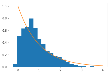
(a) Histogram of GAN’s sampling and the target density

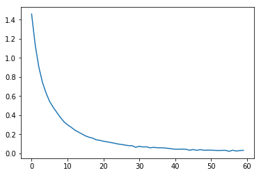
(b) Training error

Figure 1: Learning via MCMC-GAN: histogram of learned distribution and training error.

In particular, we see that the training error decreases monotonically as suggested by our theoretical results.

5 Proofs

5.1 Optimization with marginal constraint

Proof 5.1 (Proof of Theorem 3.1).

Necessary condition   Step 1. Let $\bar{\pi}^{*}\in\Pi$ be a minimizer of $V$. Since $H(\bar{\pi}^{*})<\infty$, the probability measure $\bar{\pi}^{*}$ is absolutely continuous wrt ${\rm Leb}\times{\mathsf{m}}$. Take any probability measure $\bar{\pi}\in\Pi$ such that $H(\bar{\pi})<\infty$, in particular $\bar{\pi}$ is also absolutely continuous wrt ${\rm Leb}\times{\mathsf{m}}$. Denote the convex combination by $\bar{\pi}^{\varepsilon}:=\varepsilon\bar{\pi}+(1-\varepsilon)\bar{\pi}^{*}\in\Pi$. Define the function $h(z):=z\ln z$ for $z\in\mathbb{R}^{+}$ and $h(0)=0$. Then

$$0\leq\frac{V(\bar{\pi}^{\epsilon})-V(\bar{\pi}^{*})}{\epsilon} = \frac{F(\bar{\pi}^{\epsilon})-F(\bar{\pi}^{*})}{\epsilon}+\eta\int\frac{h(\pi^{\epsilon}(x|{\mathsf{y}}))-h(\pi^{*}(x|{\mathsf{y}}))}{\varepsilon}dx{\mathsf{m}}(d{\mathsf{y}})$$

$$= \frac{1}{\epsilon}\int_{0}^{\epsilon}\int\frac{\delta F}{\delta\bar{\pi}}(\bar{\pi}^{\lambda},\bar{x})(\bar{\pi}-\bar{\pi}^{*})(d\bar{x})d\lambda+\eta\int\frac{h(\pi^{\epsilon}(x|{\mathsf{y}}))-h(\pi^{*}(x|{\mathsf{y}}))}{\varepsilon}dx{\mathsf{m}}(d{\mathsf{y}}).$$

Since $\sup_{\lambda\in[0,\varepsilon]}|\frac{\delta F}{\delta\bar{\pi}}(\bar{\pi}^{\lambda},\bar{x})|\leq C(1+|\bar{x}|^{p})$ and $\bar{\pi},\bar{\pi}^{*}\in\Pi$, by the dominated convergence theorem

$$\lim_{\varepsilon\rightarrow 0}\frac{1}{\epsilon}\int_{0}^{\epsilon}\int\frac{\delta F}{\delta\bar{\pi}}(\bar{\pi}^{\lambda},\bar{x})(\bar{\pi}-\bar{\pi}^{*})(d\bar{x})d\lambda=\int\frac{\delta F}{\delta\bar{\pi}}(\bar{\pi}^{*},\bar{x})(\bar{\pi}-\bar{\pi}^{*})(d\bar{x}).$$

Since the function $h$ is convex, we have $\frac{h(\pi^{\epsilon}(x|{\mathsf{y}}))-h(\pi^{*}(x|{\mathsf{y}}))}{\varepsilon}\leq h(\pi(x|{\mathsf{y}}))-h(\pi^{*}(x|{\mathsf{y}}))$. Note that $\int\big{(}h(\pi(x|{\mathsf{y}}))-h(\pi^{*}(x|{\mathsf{y}}))\big{)}dx{\mathsf{m}}({\mathsf{y}})=H(\bar{\pi})-H(\bar{\pi}^{*})<\infty$. By Fatou lemma, we obtain

$$\limsup_{\varepsilon\rightarrow 0}\int\frac{h(\pi^{\epsilon}(x|{\mathsf{y}}))-h(\pi^{*}(x|{\mathsf{y}}))}{\varepsilon}dx{\mathsf{m}}(d{\mathsf{y}}) \leq \int\lim_{\varepsilon\rightarrow 0}\frac{h(\pi^{\epsilon}(x|{\mathsf{y}}))-h(\pi^{*}(x|{\mathsf{y}}))}{\varepsilon}dx{\mathsf{m}}(d{\mathsf{y}})$$

$$= \int\ln\pi^{*}(x|{\mathsf{y}})(\bar{\pi}-\bar{\pi}^{*})(d\bar{x}).$$

Therefore we have

(23) $$0\leq\limsup_{\varepsilon\rightarrow 0}\frac{V(\bar{\pi}^{\epsilon})-V(\bar{\pi}^{*})}{\epsilon}\leq\int\left(\frac{\delta F}{\delta\bar{\pi}}(\bar{\pi}^{*},\bar{x})+\eta\ln\pi^{*}(x|{\mathsf{y}})\right)(\bar{\pi}-\bar{\pi}^{*})(d\bar{x}).$$

Step 2. We are going to show that for ${\mathsf{m}}$-a.s. ${\mathsf{y}}$

(24) $$\Xi_{{\mathsf{y}}}(x):=\frac{\delta F}{\delta\bar{\pi}}(\bar{\pi}^{*},\bar{x})+\eta\ln\pi^{*}(x|{\mathsf{y}})\quad\mbox{is equal to a constant $\pi^{*}(\cdot|{\mathsf{y}})$-a.s.}$$

Define the mean value $\overline{c}({\mathsf{y}}):=\int_{\mathbb{R}^{d}}\Xi_{{\mathsf{y}}}(x)\pi^{*}(dx|{\mathsf{y}})$ and let $\varepsilon,\varepsilon^{\prime}>0$. Consider the probability measure $\bar{\pi}\in\Pi$ absolutely continuous wrt $\bar{\pi}^{*}$ such that

$$\frac{d\pi(\cdot|{\mathsf{y}})}{d\pi^{*}(\cdot|{\mathsf{y}})}=\begin{cases}1,&\mbox{for ${\mathsf{y}}$ such that}\leavevmode\nobreak\ \pi^{*}\big{(}\Xi_{{\mathsf{y}}}\leq\overline{c}({\mathsf{y}})-\varepsilon\big{|}{\mathsf{y}}\big{)}<\varepsilon^{\prime}\\ \frac{1_{\Xi_{{\mathsf{y}}}\leq\overline{c}({\mathsf{y}})-\varepsilon}}{\pi^{*}\big{(}\Xi_{{\mathsf{y}}}\leq\overline{c}({\mathsf{y}})-\varepsilon\big{|}{\mathsf{y}}\big{)}},&\mbox{otherwise}\end{cases}.$$

Since $\frac{d\bar{\pi}}{d\bar{\pi}^{*}}$ is bounded, we have that $\bar{\pi}\in\Pi$ and $H(\bar{\pi})<\infty$. In particular Eq. 23 holds true for this $\bar{\pi}$. Also note that $\Xi_{{\mathsf{y}}}\leq\overline{c}({\mathsf{y}})-\varepsilon$, $\pi(\cdot|{\mathsf{y}})$-a.s. for ${\mathsf{y}}$ such that $\pi^{*}\big{(}\Xi_{{\mathsf{y}}}\leq\overline{c}({\mathsf{y}})-\varepsilon\big{|}{\mathsf{y}}\big{)}\geq\varepsilon^{\prime}$. So we have

$$0 \leq \int_{\mathbb{Y}}\int_{\mathbb{R}^{d}}\Xi_{{\mathsf{y}}}(x)\big{(}\pi(dx|{\mathsf{y}})-\pi^{*}(dx|{\mathsf{y}})\big{)}{\mathsf{m}}(d{\mathsf{y}})$$

$$= \int_{\pi^{*}\big{(}\Xi_{{\mathsf{y}}}\leq\overline{c}({\mathsf{y}})-\varepsilon\big{|}{\mathsf{y}}\big{)}\geq\varepsilon^{\prime}}\int_{\mathbb{R}^{d}}\Xi_{{\mathsf{y}}}(x)\big{(}\pi(dx|{\mathsf{y}})-\pi^{*}(dx|{\mathsf{y}})\big{)}{\mathsf{m}}(d{\mathsf{y}})$$

$$= \int_{\pi^{*}\big{(}\Xi_{{\mathsf{y}}}\leq\overline{c}({\mathsf{y}})-\varepsilon\big{|}{\mathsf{y}}\big{)}\geq\varepsilon^{\prime}}\left(\int_{\mathbb{R}^{d}}\Xi_{{\mathsf{y}}}(x)\pi(dx|{\mathsf{y}})-\overline{c}({\mathsf{y}})\right){\mathsf{m}}(d{\mathsf{y}})$$

$$\leq -\varepsilon\leavevmode\nobreak\ {\mathsf{m}}\left\{{\mathsf{y}}:\pi^{*}\big{(}\Xi_{{\mathsf{y}}}\leq\overline{c}({\mathsf{y}})-\varepsilon\big{|}{\mathsf{y}}\big{)}\geq\varepsilon^{\prime}\right\}.$$

Therefore we conclude that $\pi^{*}\big{(}\Xi_{{\mathsf{y}}}\leq\overline{c}({\mathsf{y}})-\varepsilon\big{|}{\mathsf{y}}\big{)}<\varepsilon^{\prime}$ for ${\mathsf{m}}$-a.s. ${\mathsf{y}}$. Since this is true for arbitrary $\varepsilon^{\prime},\varepsilon>0$, we obtain (24).

Step 3. We are going to show that $\bar{\pi}^{*}$ is equivalent to ${\rm Leb}\times{\mathsf{m}}$, so that $\Xi_{\mathsf{y}}$ does not depend on $x$, ${\rm Leb}\times{\mathsf{m}}$-a.s. and the first order equation Eq. 8 holds true. Suppose the opposite, i.e. there is a set ${\cal K}\in\bar{\mathbb{R}}^{d}$ such that $\bar{\pi}^{*}({\cal K})=0$ and ${\rm Leb}\times{\mathsf{m}}({\cal K})>0$. In particular, $\ln\pi^{*}(x|{\mathsf{y}})=-\infty$ on ${\cal K}$. Denote ${\cal K}_{\mathsf{y}}:=\{x\in\mathbb{R}^{d}:(x,{\mathsf{y}})\in{\cal K}\}$. We may assume that there exist $K>\varepsilon>0$ such that ${\rm Leb}({\cal K}_{\mathsf{y}})\in[\varepsilon,K]$ for all ${\mathsf{y}}\in\mathbb{Y}$. Define a probability measure $\bar{\pi}\in\Pi$ such that for all Borel-measurable $A\subset\mathbb{R}^{d}$

$$\pi(A|{\mathsf{y}}):=\frac{1}{2}\pi^{*}(A|{\mathsf{y}})+\frac{1}{2{\rm Leb}({\cal K}_{\mathsf{y}})}\int_{A\cap{\cal K}_{\mathsf{y}}}dx.$$

It is easy to verify that $H(\bar{\pi})<\infty$, so Eq. 23 holds true and it implies

$$0 \leq \frac{1}{2}\int_{\cal K}\left(\frac{\delta F}{\delta\bar{\pi}}(\bar{\pi}^{*},\bar{x})+\eta\ln\pi^{*}(x|{\mathsf{y}})\right)\bar{\pi}(d\bar{x})-\frac{1}{2}\int\left(\frac{\delta F}{\delta\bar{\pi}}(\bar{\pi}^{*},\bar{x})+\eta\ln\pi^{*}(x|{\mathsf{y}})\right)\bar{\pi}^{*}(d\bar{x})$$

$$\leq -\infty+\int C(1+|\bar{x}|^{p})\bar{\pi}^{*}(d\bar{x})-\frac{\eta}{2}H(\bar{\pi}^{*})=-\infty.$$

It is a contradiction, so $\bar{\pi}^{*}$ is equivalent to ${\rm Leb}\times{\mathsf{m}}$.

Sufficient condition  Assume that $F$ is convex. Let $\bar{\pi}^{*}\in\Pi$ satisfy the first order equation Eq. 8, in particular, $\bar{\pi}^{*}$ is equivalent to ${\rm Leb}\times{\mathsf{m}}$. Take any $\bar{\pi}\in\Pi$ absolutely continuous wrt ${\rm Leb}\times{\mathsf{m}}$ (otherwise $V(\bar{\pi})=+\infty$), and thus absolutely continuous wrt the measure $\bar{\pi}^{*}$. Define $\bar{\pi}^{\epsilon}:=(1-\epsilon)\bar{\pi}^{*}+\epsilon\bar{\pi}$ for $\epsilon>0$. By the convexity of $F$ we obtain

$$F(\bar{\pi})-F(\bar{\pi}^{*}) \geq \lim_{\varepsilon\rightarrow 0}\frac{1}{\varepsilon}\big{(}F(\bar{\pi}^{\varepsilon})-F(\bar{\pi}^{*})\big{)}$$

$$= \lim_{\varepsilon\rightarrow 0}\frac{1}{\varepsilon}\int_{0}^{\varepsilon}\int_{\bar{\mathbb{R}}^{d}}\frac{\delta F}{\delta\bar{\pi}}(\bar{\pi}^{\lambda},\bar{x})(\bar{\pi}-\bar{\pi}^{*})(d\bar{x})d\lambda=\int_{\bar{\mathbb{R}}^{d}}\frac{\delta F}{\delta\bar{\pi}}(\bar{\pi}^{*},\bar{x})(\bar{\pi}-\bar{\pi}^{*})(d\bar{x}).$$

The last equality is due to the dominated convergence theorem. On the other hand, by convexity of the function $h$,

$$H(\bar{\pi})-H(\bar{\pi}^{*})\geq\int_{\bar{\mathbb{R}}^{d}}\ln\pi^{*}(x|{\mathsf{y}})(\bar{\pi}-\bar{\pi}^{*})(d\bar{x}).$$

Hence

$$V(\bar{\pi})-V(\bar{\pi}^{*})\geq\int_{\bar{\mathbb{R}}^{d}}\bigg{(}\frac{\delta F}{\delta\bar{\pi}}(\bar{\pi}^{*},\cdot)+\eta\ln\pi^{*}(x|{\mathsf{y}})\bigg{)}(\bar{\pi}-\bar{\pi}^{*})(d\bar{x})=0,$$

so $\bar{\pi}^{*}$ is a minimizer.

5.2 Equilibria of game

Proof 5.2 (Proof of Corollary 3.4).

(i) Let $n=1$. Take three probability measures $\bar{\pi},\bar{\pi}^{\prime},\bar{\pi}^{\prime\prime}\in\Pi$ such that $\bar{\pi}=\frac{1}{2}(\bar{\pi}^{\prime}+\bar{\pi}^{\prime\prime})$. Denote $\bar{\pi}^{\prime\lambda}:=\lambda\bar{\pi}+(1-\lambda)\bar{\pi}^{\prime}$ and $\bar{\pi}^{\prime\prime\lambda}:=\lambda\bar{\pi}+(1-\lambda)\bar{\pi}^{\prime\prime}$. By the definition of the linear derivative of $F$ we obtain

$$F(\bar{\pi}^{\prime})-2F(\bar{\pi})+F(\bar{\pi}^{\prime\prime})=\int_{0}^{1}\int_{\bar{\mathbb{R}}^{N}}\frac{\delta F}{\delta\nu}(\bar{\pi}^{\prime\lambda},\bar{x})(\bar{\pi}^{\prime}-\bar{\pi})(d\bar{x})d\lambda+\int_{0}^{1}\int_{\bar{\mathbb{R}}^{N}}\frac{\delta F}{\delta\nu}(\bar{\pi}^{\prime\prime\lambda},\bar{x})(\bar{\pi}^{\prime\prime}-\bar{\pi})(d\bar{x})d\lambda.$$

Note that $\bar{\pi}^{\prime}-\bar{\pi}=\bar{\pi}-\bar{\pi}^{\prime\prime}=\frac{1}{2-2\lambda}\big{(}\bar{\pi}^{\prime\lambda}-\bar{\pi}^{\prime\prime\lambda}\big{)}$. Therefore we have

$$F(\bar{\pi}^{\prime})-2F(\bar{\pi})+F(\bar{\pi}^{\prime\prime})=\int_{0}^{1}\frac{1}{2-2\lambda}\int_{\bar{\mathbb{R}}^{N}}\left(\frac{\delta F}{\delta\nu}(\bar{\pi}^{\prime\lambda},\bar{x})-\frac{\delta F}{\delta\nu}(\bar{\pi}^{\prime\prime\lambda},\bar{x})\right)(\bar{\pi}^{\prime\lambda}-\bar{\pi}^{\prime\prime\lambda})(d\bar{x})d\lambda\geq 0.$$

Finally note that $\lambda\mapsto(F(\bar{\pi}^{\prime\lambda}),F(\bar{\pi}^{\prime\prime\lambda}))$ is continuous. So $F$ satisfying the monotonicity condition must be convex on $\Pi$.

On the other hand, suppose $F$ is convex on $\Pi$. Following a similar computation, we obtain

$$0\leq\frac{1}{\varepsilon}\Big{(}F(\bar{\pi}^{\prime})-F(\bar{\pi}^{\prime\varepsilon})-F(\bar{\pi}^{\prime\prime\varepsilon})+F(\bar{\pi}^{\prime\prime})\Big{)}\\ =\frac{1}{\varepsilon}\int_{0}^{\varepsilon}\frac{1}{2}\int_{\bar{\mathbb{R}}^{N}}\left(\frac{\delta F}{\delta\nu}(\bar{\pi}^{\prime\lambda},\bar{x})-\frac{\delta F}{\delta\nu}(\bar{\pi}^{\prime\prime\lambda},\bar{x})\right)(\bar{\pi}^{\prime}-\bar{\pi}^{\prime\prime})(d\bar{x})d\lambda.$$

Let $\bar{\pi}^{\prime},\bar{\pi}^{\prime\prime}\in\Pi$. It follows from the dominated convergence theorem that

$$0 \leq \lim_{\varepsilon\rightarrow 0}\frac{1}{\varepsilon}\int_{0}^{\varepsilon}\frac{1}{2}\int_{\bar{\mathbb{R}}^{N}}\left(\frac{\delta F}{\delta\nu}(\bar{\pi}^{\prime\lambda},\bar{x})-\frac{\delta F}{\delta\nu}(\bar{\pi}^{\prime\prime\lambda},\bar{x})\right)(\bar{\pi}^{\prime}-\bar{\pi}^{\prime\prime})(d\bar{x})d\lambda$$

$$= \frac{1}{2}\int_{\bar{\mathbb{R}}^{N}}\left(\frac{\delta F}{\delta\nu}(\bar{\pi}^{\prime},\bar{x})-\frac{\delta F}{\delta\nu}(\bar{\pi}^{\prime\prime},\bar{x})\right)(\bar{\pi}^{\prime}-\bar{\pi}^{\prime\prime})(d\bar{x}).$$

So $F$ satisfies the monotonicity condition on $\Pi$.

(ii) Let $\bar{\pi}^{*}\in\Pi$ be a Nash equilibrium of the game. Then, by Corollary 3.3 we have that for every $i$ there exists a function $f^{i}:\mathbb{Y}\rightarrow\mathbb{R}$

$$\frac{\delta F^{i}}{\delta\nu}((\bar{\pi}^{*})^{i},(\bar{\pi}^{*})^{-i},x^{i},{\mathsf{y}})+\frac{\sigma^{2}}{2}\ln((\pi^{*})^{i}(x^{i}|{\mathsf{y}}))=f^{i}({\mathsf{y}}),\quad\mbox{for ${\mathsf{m}}$-a.s. ${\mathsf{y}}$.}$$

Let $\bar{\pi}^{*},\bar{\pi}^{\prime*}\in\Pi$ be Nash equilibriums. Then monotonicity condition Corollary 3.4 implies

$$\sum_{i=1}^{n}\int\limits_{\bar{\mathbb{R}}^{N}}\left(-\frac{\sigma^{2}}{2}\ln((\pi^{*})^{i}(x^{i}|{\mathsf{y}}))+\frac{\sigma^{2}}{2}\ln((\pi^{\prime*})^{i}(x^{i}|{\mathsf{y}}))\right)(\bar{\pi}^{*}-\bar{\pi}^{\prime*})(d\bar{x})\geq 0,$$

because the marginal distributions of $\bar{\pi}^{*}$ and $\bar{\pi}^{\prime*}$ on $\mathbb{Y}$ coincide. The latter inequality can be rewritten

$$0 \leq -\sum_{i=1}^{n}\int\limits_{\bar{\mathbb{R}}^{n^{i}}}\ln\left(\frac{(\pi^{*})^{i}(x^{i}|{\mathsf{y}})}{(\pi^{\prime*})^{i}(x^{i}|{\mathsf{y}})}\right)((\bar{\pi}^{*})^{i}-(\bar{\pi}^{\prime*})^{i})(d\bar{x}^{i})$$

$$= -\sum_{i=1}^{n}\left(H((\bar{\pi}^{*})^{i}|(\bar{\pi}^{\prime*})^{i})+H((\bar{\pi}^{\prime*})^{i}|(\bar{\pi}^{*})^{i})\right).$$

This is only possible if $(\bar{\pi}^{*})^{i}=(\bar{\pi}^{\prime*})^{i}$ for all $i=1,\ldots,n$.

Proof 5.3 (Proof of Theorem 3.6).

For $\bar{\pi}\in\Pi$ denote ${\cal R}^{i}(\bar{\pi}):=\operatorname*{\arg\!\min}_{\nu\in\Pi^{i}}V^{i}(\nu,\bar{\pi}^{-i})$ for $i=1,\cdots,n$, and define

$${\cal R}(\bar{\pi}):=\{\bar{\pi}^{\prime}\in\Pi:\leavevmode\nobreak\ \bar{\pi}^{\prime i}\in{\cal R}^{i}(\bar{\pi})\leavevmode\nobreak\ \mbox{for $i=1,\cdots,n$}\}.$$

Step 1. First we prove that ${\cal R}(\bar{\pi})$ is ${\cal W}_{p}$-compact. For any $\nu^{i}\in{\cal R}^{i}(\bar{\pi})$, it follows from the first order equation Eq. 8 that

$$\nu^{i}(\bar{x}^{i})=C(\nu^{i},\bar{\pi}^{-i})e^{-\frac{2}{\sigma^{2}}\frac{\delta F^{i}}{\delta\nu}(\nu^{i},\bar{\pi}^{-i},\bar{x}^{i})},$$

where $C(\nu^{i},\bar{\pi}^{-i})>0$ is the normalization constant so that $\nu^{i}$ is a probability measure. Take a $p^{\prime}>p$. The condition (10) implies that $C(\nu^{i},\bar{\pi}^{-i})$ is uniformly bounded as well as

$$\int_{\bar{\mathbb{R}}^{n^{i}}}|\bar{x}^{i}|^{p^{\prime}}\nu^{i}(d\bar{x}^{i})\leq C(\nu^{i},\bar{\pi}^{-i})\int_{\bar{\mathbb{R}}^{n^{i}}}|\bar{x}^{i}|^{p^{\prime}}e^{-C^{\prime}|\bar{x}^{i}|^{q}+C}dx^{i}{\mathsf{m}}(d{\mathsf{y}}).$$

So we have

$$\overline{C}^{i}:=\sup_{\nu^{i}\in{\cal R}^{i}(\bar{\pi})}\int_{\bar{\mathbb{R}}^{n^{i}}}|\bar{x}^{i}|^{p^{\prime}}\nu^{i}(d\bar{x}^{i})<\infty.$$

Therefore, ${\cal R}(\bar{\pi})\subset{\cal E}:=\{\nu\in\Pi:\nu^{i}\in{\cal E}^{i}\mbox{ for $i=1,\cdots,n$}\}$, with ${\cal E}^{i}:=\{\nu^{i}\in\Pi^{i}:\int_{\bar{\mathbb{R}}^{n^{i}}}|\bar{x}^{i}|^{p^{\prime}}\nu^{i}(d\bar{x}^{i})\leq\overline{C}^{i}\}$, and note that ${\cal E}$ is ${\cal W}_{p}$-compact.

Step 2. We are going to show that the graph of $\bar{\pi}\in{\cal E}\mapsto{\cal R}(\bar{\pi})$ is ${\cal W}_{p}$-closed, i.e. given $\bar{\pi}_{m},\bar{\pi}_{\infty}\in\Pi\cap{\cal E}$, $\bar{\pi}^{\prime}_{m}\in{\cal R}(\bar{\pi}_{m})$ such that $\bar{\pi}_{m}\rightarrow\bar{\pi}_{\infty}$ in ${\cal W}_{p}$ and $\bar{\pi}^{\prime}_{m}\rightarrow\bar{\pi}^{\prime}_{\infty}\in\Pi$, we want to show that $\bar{\pi}^{\prime}_{\infty}\in{\cal R}(\bar{\pi}_{\infty})$.

Denote the concatenation of two probability measures $\nu^{i}\in\Pi^{i},\mu^{-i}\in\Pi^{-i}$ by

$$\nu^{i}\otimes\mu^{-i}(dx,d{\mathsf{y}})=\nu^{i}(x^{i}|{\mathsf{y}})\mu^{-i}(x^{-i}|{\mathsf{y}})dx{\mathsf{m}}(d{\mathsf{y}}).$$

Note that for $\bar{\pi},\bar{\pi}^{\prime}\in{\cal E}$ we have $\bar{\pi}^{\prime i}\otimes\bar{\pi}^{-i}\in{\cal E}$. Since ${\cal E}$ is ${\cal W}_{p}$-compact, there is a subsequence, still denoted by $(\bar{\pi}_{m},\bar{\pi}^{\prime}_{m})$, and $\bar{\pi}^{*}\in\Pi\cap{\cal E}$ such that $\bar{\pi}^{\prime i}_{m}\otimes\bar{\pi}^{-i}_{m}\rightarrow\bar{\pi}^{*}$ in ${\cal W}_{p}$ and $\bar{\pi}^{*,i}=\bar{\pi}^{\prime i}_{\infty}$, $\bar{\pi}^{*,-i}=\bar{\pi}^{-i}_{\infty}$. By the lower-semicontinuity of the mapping: $\bar{\pi}\mapsto V^{i}(\bar{\pi}^{i},\bar{\pi}^{-i})$, we have

(25) $$V^{i}(\bar{\pi}^{\prime i}_{\infty},\bar{\pi}^{-i}_{\infty})=V^{i}(\bar{\pi}^{*,i},\bar{\pi}^{*,-i})\leq\liminf_{m\rightarrow\infty}V^{i}(\bar{\pi}^{\prime i}_{m},\bar{\pi}^{-i}_{m}).$$

Further, fix $\nu^{i}\in\Pi^{i}\cap{\cal E}^{i}$. Again by the compactness of ${\cal E}$, there is a subsequence, still denoted by $(\nu^{i},\bar{\pi}^{\prime}_{m})$, and $\bar{\pi}^{\nu}\in\Pi\cap{\cal E}$ such that $\nu^{i}\otimes\bar{\pi}^{-i}_{m}\rightarrow\bar{\pi}^{\nu}$ in ${\cal W}_{p}$ and $\bar{\pi}^{\nu,i}=\nu^{i}$, $\bar{\pi}^{\nu,-i}=\bar{\pi}^{-i}_{\infty}$. Therefore

$$\liminf_{m\rightarrow\infty}V^{i}(\bar{\pi}^{\prime i}_{m},\bar{\pi}^{-i}_{m})\leq\liminf_{m\rightarrow\infty}V^{i}(\nu^{i},\bar{\pi}^{-i}_{m})=V^{i}(\bar{\pi}^{\nu,i},\bar{\pi}^{\nu,-i})=V^{i}(\nu^{i},\bar{\pi}^{-i}_{\infty}).$$

Together with Eq. 25, we conclude that $\bar{\pi}^{{}^{\prime}i}_{\infty}\in{\cal R}^{i}(\bar{\pi}_{\infty})$ for all $i$, and thus $\bar{\pi}^{\prime}_{\infty}\in{\cal R}(\bar{\pi}_{\infty})$.

Step 3. From the condition of the theorem and the result of Step 1&2, we conclude that for any $\bar{\pi}\in\Pi$ the set ${\cal R}(\bar{\pi})$ is non-empty, convex, that the set $\cup_{\bar{\pi}\in\Pi}{\cal R}(\bar{\pi})$ is a subset of a ${\cal W}_{p}$-compact set, and that the graph of the mapping $\bar{\pi}\in{\cal E}\mapsto{\cal R}(\bar{\pi})\subset{\cal E}$ is ${\cal W}_{p}$-closed. Therefore, it follows from the Kakutani fixed-point theorem that the mapping $\bar{\pi}\mapsto{\cal R}(\bar{\pi})$ has a fixed point, which is a Nash equilibrium.

5.3 Invariant measure of MFL system

Proof 5.4 (Proof of Theorem 3.8).

The proof is based on the Banach fixed point theorem. Given fixed $(\bar{\pi}_{t}),(\bar{\pi}^{\prime}_{t})\in\overline{C}_{p}([0,T],\Pi)$, the SDEs Eq. 5 apparently have unique strong solutions, denoted by $\bar{X},\bar{X}^{\prime}$ respectively. Denote by $\hat{\bar{\pi}}_{t}:={\rm Law}(\bar{X}_{t})$ and $\hat{\bar{\pi}}^{\prime}_{t}:={\rm Law}(\bar{X}^{\prime}_{t})$. We are going to show that the mapping $\Psi:\bar{\pi}\mapsto\hat{\bar{\pi}}$ is a contraction as $T$ is small enough.

First, by the standard SDE estimate we know $\mathbb{E}\big{[}\sup_{t\in[0,T]}|X_{t}|^{p}\big{]}<\infty$, and this implies $(\hat{\bar{\pi}}_{t}),(\hat{\bar{\pi}}^{\prime}_{t})\in\overline{C}_{p}([0,T],\Pi)$. Note the SDEs for $\tilde{X},\tilde{X}^{\prime}$ share the same Brownian motion. Denoting $\delta X=X-X^{\prime}$, we have

$$|\delta X^{i}_{s}|^{p} = \left|\int_{0}^{s}\left(-\nabla_{x^{i}}\frac{\delta F^{i}}{\delta\nu}(\bar{\pi}^{i}_{t},\bar{\pi}^{-i}_{t},X^{i}_{t},Y)+\nabla_{x^{i}}\frac{\delta F^{i}}{\delta\nu}(\bar{\pi}^{\prime i}_{t},\bar{\pi}^{\prime-i}_{t},X^{\prime i}_{t},Y)dt\right)dt\right|^{p}$$

$$\leq T^{1-\frac{1}{p}}\Big{(}\int_{0}^{s}C\Big{(}{\cal W}_{p}^{p}(\bar{\pi}^{i}_{t},\bar{\pi}^{\prime i}_{t})+{\cal W}_{p}^{p}(\bar{\pi}^{-i}_{t},\bar{\pi}^{\prime-i}_{t})+|\delta X^{i}_{t^{\prime}}|^{p}\Big{)}dt+\int_{0}^{s}C_{0}{\cal W}_{p}^{p}(\bar{\pi}^{-i}_{t}(\cdot|Y),\bar{\pi}^{\prime-i}_{t}(\cdot|Y))dt\Big{)}.$$

Taking expectation on both sides, by the Gronwall inequality we obtain that

$$\mathbb{E}\big{[}|\delta X^{\mathsf{y}}_{s}|^{p}\big{]}\leq Ce^{CT}\int_{0}^{T}\Big{(}{\cal W}^{p}_{p}(\bar{\pi}_{t},\bar{\pi}^{\prime}_{t})+{\cal W}^{p}_{p}(\bar{\pi}_{t}(\cdot|{\mathsf{y}}),\bar{\pi}^{\prime}_{t}(\cdot|{\mathsf{y}}))\Big{)}dt.$$

Note that $\mathbb{E}\big{[}|\delta X^{\mathsf{y}}_{s}|^{p}\big{]}\geq{\cal W}_{p}^{p}(\hat{\bar{\pi}}_{s}(\cdot|{\mathsf{y}}),\hat{\bar{\pi}}^{\prime}_{s}(\cdot|{\mathsf{y}}))$. Therefore

$${\cal W}_{p}^{p}(\hat{\bar{\pi}}_{s}(\cdot|{\mathsf{y}}),\hat{\bar{\pi}}^{\prime}_{s}(\cdot|{\mathsf{y}}))\leq Ce^{CT}\int_{0}^{T}\Big{(}{\cal W}^{p}_{p}(\bar{\pi}_{t},\bar{\pi}^{\prime}_{t})+{\cal W}^{p}_{p}(\bar{\pi}_{t}(\cdot|{\mathsf{y}}),\bar{\pi}^{\prime}_{t}(\cdot|{\mathsf{y}}))\Big{)}dt.$$

Integrating both sides with respect to ${\mathsf{m}}$, we obtain

$$\overline{\cal W}_{p}^{p}(\hat{\bar{\pi}}_{t},\hat{\bar{\pi}}^{\prime}_{t})\leq Ce^{CT}\int_{0}^{T}2\overline{\cal W}^{p}_{p}(\bar{\pi}_{t},\bar{\pi}^{\prime}_{t})dt\leq 2CTe^{CT}\sup_{t\in[0,T]}\overline{\cal W}^{p}_{p}(\bar{\pi}_{t},\bar{\pi}^{\prime}_{t}),$$

and $\Psi$ is a contraction whenever $T$ is small enough. In case $C_{0}=0$ the result can be deduced similarly.

In order to prove Theorem 3.10, the main ingredient is the reflection coupling in Eberle [10]. For this mean-field system, we shall adopt the reflection-synchronous coupling as in [11].

We first recall the reflection-synchronous coupling. Fix a parameter $\varepsilon>0$. Introduce the Lipschitz functions ${\rm rc}:\mathbb{R}^{N}\times\mathbb{R}^{N}\rightarrow[0,1]$ and ${\rm sc}:\mathbb{R}^{N}\times\mathbb{R}^{N}\rightarrow[0,1]$ satisfying

$${\rm sc}^{2}(x,x^{\prime})+{\rm rc}^{2}(x,x^{\prime})=1,\quad{\rm rc}(x,x^{\prime})=1\leavevmode\nobreak\ \leavevmode\nobreak\ \mbox{for $|x-x^{\prime}|\geq\varepsilon$},\quad{\rm rc}(x,x^{\prime})=0\leavevmode\nobreak\ \leavevmode\nobreak\ \mbox{for $|x-x^{\prime}|\leq\varepsilon/2$}.$$

Let $\bar{\pi}_{0},\bar{\pi}^{\prime}_{0}\in\Pi\cap{\cal P}_{q}(\bar{\mathbb{R}}^{N})$ with some $q>1$ be two initial distributions of the MFL system Eq. 5, and $W,\tilde{W}$ be two independent $N$-dimensional Brownian motions. It follows from Theorem 3.8 the two MFL systems have strong solutions, and denote the marginal laws by $\bar{\pi}_{t},\bar{\pi}^{\prime}_{t}$. Denote the drift of the dynamics Eq. 6 by

(26) $$b^{\mathsf{y}}(t,x):=\left(-\nabla_{x^{i}}\frac{\delta F^{i}}{\delta\nu}(\bar{\pi}^{i}_{t},\bar{\pi}^{-i}_{t},x^{i},{\mathsf{y}})\right)_{i=1,\cdots,n},\quad\tilde{b}^{\mathsf{y}}(t,x):=\left(-\nabla_{x^{i}}\frac{\delta F^{i}}{\delta\nu}(\bar{\pi}^{\prime i}_{t},\bar{\pi}^{\prime-i}_{t},x^{i},{\mathsf{y}})\right)_{i=1,\cdots,n}$$

Further, for a fixed ${\mathsf{y}}\in\mathbb{Y}$, define the coupling $\Sigma^{\mathsf{y}}=(X^{\mathsf{y}},X^{\prime{\mathsf{y}}})$ as the strong solution to the SDE

$$dX^{\mathsf{y}}_{t}=b^{\mathsf{y}}(t,X^{\mathsf{y}}_{t})dt+{\rm rc}(\Sigma^{\mathsf{y}}_{t})\sigma dW_{t}+{\rm sc}(\Sigma^{\mathsf{y}}_{t})\sigma d\tilde{W}_{t},$$

$$dX^{\prime{\mathsf{y}}}_{t}=\tilde{b}^{\mathsf{y}}(t,X^{\prime{\mathsf{y}}}_{t})dt+{\rm rc}(\Sigma^{\mathsf{y}}_{t})\big{(}{\rm Id}-2e_{t}\langle e_{t},\cdot\rangle\big{)}\sigma dW_{t}+{\rm sc}(\Sigma^{\mathsf{y}}_{t})\sigma d\tilde{W}_{t},$$

where $e_{t}:=\frac{X^{\mathsf{y}}_{t}-X^{\prime{\mathsf{y}}}_{t}}{|X^{\mathsf{y}}_{t}-X^{\prime{\mathsf{y}}}_{t}|}$ for $X^{\mathsf{y}}_{t}\neq X^{\prime{\mathsf{y}}}_{t}$, otherwise $e_{t}:=\hat{e}$ some arbitrary fixed unit vector in $\mathbb{R}^{N}$.

In the following proof, we will use the concave increasing function $f$ constructed in [11, Theorem 2.3]:

$$f(r):=\int_{0}^{r}\varphi(s)g(s\wedge R_{2})ds,\quad\mbox{where}\quad g(r):=1-\frac{c}{2}\int_{0}^{r}\Phi(s)\varphi(s)^{-1}ds,$$

and the function $\varphi$ and the constants $R_{2},c$ are defined in the statement of Theorem 3.10. In particular, on $(0,R_{2})\cup(R_{2},+\infty)$ the function $f$ satisfies

(27) $$2\sigma^{2}f^{\prime\prime}(r)\leq-r\big{(}\kappa(r)+2\gamma\eta(r)\big{)}f^{\prime}(r)-c\sigma^{2}f(r)$$

and for $r\in\mathbb{R}^{+}$

(28) $$r\varphi(R_{1})\leq\Phi(r)\leq 2f(r)\leq 2\Phi(r)\leq 2r.$$

Proof 5.5 (Proof of Theorem 3.10).

Note that $\pi_{0}(\cdot|{\mathsf{y}}),\pi^{\prime}_{0}(\cdot|{\mathsf{y}})\in{\cal P}_{q}(\mathbb{R}^{N})$ with $q>1$ for ${\mathsf{m}}$-a.s. ${\mathsf{y}}\in\mathbb{Y}$. For such ${\mathsf{y}}$, we may choose the coupling $(X^{\mathsf{y}}_{0},X^{\prime{\mathsf{y}}}_{0})$ so that

(29) $${\cal W}_{1}\big{(}\pi_{0}(\cdot|{\mathsf{y}}),\pi^{\prime}_{0}(\cdot|{\mathsf{y}})\big{)}=\mathbb{E}\big{[}|X^{\mathsf{y}}_{0}-X^{\prime{\mathsf{y}}}_{0}|\big{]}\geq\mathbb{E}\Big{[}f\big{(}|X^{\mathsf{y}}_{0}-X^{\prime{\mathsf{y}}}_{0}|\big{)}\Big{]}.$$

The last inequality is due to (28). On the other hand, for all $t\geq 0$ we have

(30) $${\cal W}_{1}\big{(}\pi_{t}(\cdot|{\mathsf{y}}),\pi^{\prime}_{t}(\cdot|{\mathsf{y}})\big{)}\leq\mathbb{E}\big{[}|X^{\mathsf{y}}_{t}-X^{\prime{\mathsf{y}}}_{t}|\big{]}\leq\frac{2}{\varphi(R_{1})}\mathbb{E}\Big{[}f\big{(}|X^{\mathsf{y}}_{t}-X^{\prime{\mathsf{y}}}_{t}|\big{)}\Big{]}.$$

Denote $\delta X^{\mathsf{y}}_{t}:=X^{\mathsf{y}}_{t}-X^{\prime{\mathsf{y}}}_{t}$. By the definition of the coupling above, we have

$$d\delta X^{\mathsf{y}}_{t}=\Big{(}b^{\mathsf{y}}(t,X^{\mathsf{y}}_{t})-\tilde{b}^{\mathsf{y}}(t,X^{\prime{\mathsf{y}}}_{t})\Big{)}dt+2{\rm rc}(\Sigma^{\mathsf{y}}_{t})\sigma e_{t}d\bar{W}_{t},$$

where $\bar{W}_{t}:=\int_{0}^{t}e_{s}\cdot dW_{s}$ is a one-dimensional Brownian motion. Denote $r_{t}:=|\delta X^{\mathsf{y}}_{t}|$ and note that by the definition of ${\rm rc}$ we have ${\rm rc}(\Sigma^{\mathsf{y}}_{t})=0$ whenever $r_{t}\leq\varepsilon/2$. Therefore,

$$dr_{t}=e_{t}\cdot\Big{(}b^{\mathsf{y}}(t,X^{\mathsf{y}}_{t})-\tilde{b}^{\mathsf{y}}(t,X^{\prime{\mathsf{y}}}_{t})\Big{)}dt+2{\rm rc}(\Sigma^{\mathsf{y}}_{t})\sigma d\bar{W}_{t}.$$

Then it follows from the Itô-Tanaka formula and the concavity of $f$ that

$$f(r_{t})-f(r_{0}) \leq \int_{0}^{t}\left(f^{\prime}(r_{s})e_{s}\cdot\big{(}b^{\mathsf{y}}(s,X^{\mathsf{y}}_{s})-\tilde{b}^{\mathsf{y}}(s,X^{\prime{\mathsf{y}}}_{s})\big{)}+2{\rm rc}(\Sigma^{\mathsf{y}}_{s})^{2}\sigma^{2}f^{\prime\prime}(r_{s})\right)ds+M_{t},$$

where $M_{t}:=2\int_{0}^{t}{\rm rc}(\Sigma^{\mathsf{y}}_{s})f^{\prime}(r_{s})\sigma d\bar{W}_{s}$ is a martingale. Now note that

$$e_{s}\cdot\big{(}b^{\mathsf{y}}(s,X^{\mathsf{y}}_{s})-\tilde{b}^{\mathsf{y}}(s,X^{\prime{\mathsf{y}}}_{s})\big{)}\leq 1_{\{r_{s}\geq\varepsilon\}}r_{s}\kappa(r_{s})+1_{\{r_{s}<\varepsilon\}}C\varepsilon+\gamma\big{(}\overline{\cal W}_{1}(\bar{\pi}_{s},\bar{\pi}^{\prime}_{s})+{\cal W}_{1}(\pi_{s}(\cdot|{\mathsf{y}}),\pi^{\prime}_{s}(\cdot|{\mathsf{y}}))\big{)}.$$

Further, since $f^{\prime\prime}\leq 0$ and ${\rm rc}(\Sigma^{\mathsf{y}}_{s})=1$ whenever $r_{s}\geq\varepsilon$, we have

$$f(r_{t})-f(r_{0}) \leq \int_{0}^{t}\Big{(}1_{\{r_{s}\geq\varepsilon\}}\big{(}f^{\prime}(r_{s})r_{s}\kappa(r_{s})+2\sigma^{2}f^{\prime\prime}(r_{s})\big{)}+1_{\{r_{s}<\varepsilon\}}C\varepsilon$$

$$\quad\quad\quad\quad\quad\quad\quad+\gamma f^{\prime}(r_{s})\big{(}\overline{\cal W}_{1}(\bar{\pi}_{s},\bar{\pi}^{\prime}_{s})+{\cal W}_{1}(\pi_{s}(\cdot|{\mathsf{y}}),\pi^{\prime}_{s}(\cdot|{\mathsf{y}}))\big{)}\Big{)}ds+M_{t}.$$

By taking expectation on both sides, we obtain

$$\int\mathbb{E}\Big{[}f(r_{t})-f(r_{0})\Big{]}{\mathsf{m}}(d{\mathsf{y}})$$

$$\leq \int_{0}^{t}\Big{(}\int\mathbb{E}\Big{[}1_{\{r_{s}\geq\varepsilon\}}\big{(}f^{\prime}(r_{s})r_{s}\kappa(r_{s})+2\sigma^{2}f^{\prime\prime}(r_{s})\big{)}+C\varepsilon\Big{]}{\mathsf{m}}(d{\mathsf{y}})+2\gamma f^{\prime}(r_{s})\overline{\cal W}_{1}(\bar{\pi}_{s},\bar{\pi}^{\prime}_{s})\Big{)}ds$$

$$\leq \int_{0}^{t}\Big{(}\int\mathbb{E}\Big{[}-c\sigma^{2}f(r_{s})1_{\{r_{s}\geq\varepsilon\}}+C\varepsilon\Big{]}{\mathsf{m}}(d{\mathsf{y}})+2\gamma\overline{\cal W}_{1}(\bar{\pi}_{s},\bar{\pi}^{\prime}_{s})\Big{)}ds$$

$$\leq \int_{0}^{t}\Big{(}\int\mathbb{E}\Big{[}-c\sigma^{2}f(r_{s})+(C+c\sigma^{2})\varepsilon\Big{]}{\mathsf{m}}(d{\mathsf{y}})+2\gamma\overline{\cal W}_{1}(\bar{\pi}_{s},\bar{\pi}^{\prime}_{s})\Big{)}ds.$$

The second last inequality is due to (27). Together with (29) and (30), we obtain

$$\frac{\varphi(R_{1})}{2}e^{c\sigma^{2}t}\overline{\cal W}_{1}\big{(}\bar{\pi}_{t},\bar{\pi}^{\prime}_{t}\big{)}-\overline{\cal W}_{1}\big{(}\bar{\pi}_{0},\bar{\pi}^{\prime}_{0}\big{)} \leq e^{c\sigma^{2}t}\int\mathbb{E}\big{[}f(r_{t})\big{]}{\mathsf{m}}(d{\mathsf{y}})-\int\mathbb{E}\big{[}f(r_{0})\big{]}{\mathsf{m}}(d{\mathsf{y}})$$

$$\leq \int_{0}^{t}e^{c\sigma^{2}s}\big{(}(C+c\sigma^{2})\varepsilon+2\gamma\overline{\cal W}_{1}(\bar{\pi}_{s},\bar{\pi}^{\prime}_{s})\big{)}ds.$$

This holds true for all $\varepsilon>0$, so finally we obtain Eq. 12 by Gronwall’s inequality.

5.4 One player case

Throughout this subsection, we suppose that the assumptions in Theorem 3.11 hold true. Recall the drift function $b^{\mathsf{y}}$ defined in Eq. 26 with $n=1$, i.e.

$$b^{\mathsf{y}}(t,x):=-\nabla_{x}\frac{\delta F}{\delta\nu}(\bar{\pi}_{t},x,{\mathsf{y}}).$$

Under the assumption of Theorem 3.11 the function $b^{\mathsf{y}}$ is continuous in $(t,x)$ and $C^{3}$ in $x$ for all $t\in[0,T]$. Due to a classical regularity result in the theory of linear PDEs (see e.g. [18, p.14-15]), we obtain the following result.

Lemma 5.6.

Under the assumption of Theorem 3.11, the marginal laws $(\pi_{t}(\cdot|{\mathsf{y}}))_{t\geq 0}$ of the solution to Eq. 6 are weakly continuous solutions to the Fokker-Planck equations:

(31) $$\partial_{t}\nu=\nabla_{x}\cdot(-b^{\mathsf{y}}\nu+\frac{\sigma^{2}}{2}\nabla_{x}\nu)\quad\mbox{for}\quad{\mathsf{y}}\in\mathbb{Y}.$$

In particular, we have that $(t,x)\mapsto\pi_{t}(x|{\mathsf{y}})$ belongs to $C^{1,2}\big{(}(0,\infty)\times\mathbb{R}^{N})\big{)}$.

The following results can be proved with the same argument as in Lemma 5.5-5.7 in [15], so the proof is omitted.

Lemma 5.7.

Fix a ${\mathsf{y}}\in\mathbb{Y}$ and assume $\mathbb{E}\big{[}|X^{\mathsf{y}}_{0}|^{2}\big{]}<\infty$, where we recall the $X^{\mathsf{y}}$ defined in Eq. 6. Denote by $\mathbb{Q}^{\sigma}_{\mathsf{y}}$ the scaled Wiener measure with initial distribution $\pi_{0}(\cdot|{\mathsf{y}})$ and by $({\cal F}_{t})_{t\geq 0}$ the canonical filtration of the Wiener space. Then

1. for any finite horizon $T>0$, the law of the solution to Eq. 5, $\mathbf{\Pi}(\cdot|{\mathsf{y}}):={\rm Law}(X^{\mathsf{y}})$, is equivalent to $\mathbb{Q}^{\sigma}_{\mathsf{y}}$ on ${\cal F}_{T}$ and the relative entropy

   $$\int\ln\Big{(}\frac{d\mathbf{\Pi}(\cdot|{\mathsf{y}})}{d\mathbb{Q}^{\sigma}_{\mathsf{y}}}\Big{|}_{{\cal F}_{T}}\Big{)}d\nu_{t}=\mathbb{E}\Big{[}\int_{0}^{T}\big{|}b^{\mathsf{y}}(t,X^{\mathsf{y}}_{t})\big{|}^{2}dt\Big{]}<+\infty.$$

2. the marginal law $\pi_{t}(\cdot|{\mathsf{y}})$ admits a density s.t. $\pi_{t}(\cdot|{\mathsf{y}})>0$ and $H\big{(}\pi_{t}(\cdot|{\mathsf{y}})\big{)}<+\infty$ for $t>0$.

3. the function $\ln\pi_{t}(x|{\mathsf{y}})$ is continuous differentiable in $x$ for $t>0$, and for any $t_{0}\in(0,t]$ it satisfies

   $$\nabla_{x}\ln\pi_{t}(x|{\mathsf{y}})=-\frac{1}{t_{0}}\mathbb{E}\left[\int_{0}^{t_{0}}\big{(}1-s\nabla_{x}b^{\mathsf{y}}(s,X^{\mathsf{y}}_{t-t_{0}+s})\big{)}dW^{t-t_{0}}_{s}\Big{|}X^{\mathsf{y}}_{t}=x\right],$$

   where $W^{t-t_{0}}_{s}:=W_{t-t_{0}+s}-W_{t-t_{0}}$ and $W$ is the Brownian motion in Eq. 6. In particular, for any $t_{*}>0$ we have

   $$C:=\sup_{s\geq t_{*}}\int_{\mathbb{R}^{N}}\big{|}\nabla_{x}\ln\pi_{s}(x|{\mathsf{y}})\big{|}^{2}\pi_{s}(x|{\mathsf{y}})dx<+\infty,$$

   and $C$ only depends on $t_{*}$ and the Lipschitz constant of $\nabla_{x}b^{\mathsf{y}}$ with respect to $x$.

4. we have the estimates

   $$\int_{\mathbb{R}^{N}}|\nabla_{x}\ln\pi_{t}(x|{\mathsf{y}})|dx<+\infty,\quad\int_{\mathbb{R}^{N}}|x\cdot\nabla_{x}\ln\pi_{t}(x|{\mathsf{y}})|dx<+\infty\quad\mbox{for all}\quad t>0,$$

   $$\mbox{and}\quad\int_{t}^{t^{\prime}}\int_{\mathbb{R}^{N}}|\Delta_{xx}\pi_{s}(x|{\mathsf{y}})|dxds<+\infty\quad\mbox{for all}\quad t^{\prime}>t>0,$$

   and together with the integration by parts we obtain for all $t^{\prime}>t>0$

   (32) $$\int_{\mathbb{R}^{N}}\Delta_{xx}\frac{\delta F}{\delta\nu}(\bar{\pi}_{t},x,{\mathsf{y}})\pi_{t}(x|{\mathsf{y}})dx=-\int_{\mathbb{R}^{N}}\nabla_{x}\frac{\delta F}{\delta\nu}(\bar{\pi}_{t},x,{\mathsf{y}})\cdot\nabla_{x}\pi_{t}(x|{\mathsf{y}})dx,$$

   $$\int_{t}^{t^{\prime}}\int_{\mathbb{R}^{N}}\Delta_{xx}\big{(}\ln\pi_{s}(x|{\mathsf{y}})\big{)}\pi_{s}(x|{\mathsf{y}})dxds=-\int_{t}^{t^{\prime}}\int_{\mathbb{R}^{N}}\left|\nabla_{x}\ln\pi_{s}(x|{\mathsf{y}})\right|^{2}\pi_{s}(x|{\mathsf{y}})dxds.$$

The proof of Theorem 3.11 is based on the previous lemma and Itô calculus.

Proof 5.8 (Proof of Theorem 3.11).

It follows from the Itô-type formula [2, Theorem 4.14] and (32) that

(33) $$\mathrm{d}F(\bar{\pi}_{t}) = \int_{\mathbb{R}^{N}}\left(-\big{|}\nabla_{x}\frac{\delta F}{\delta\nu}(\bar{\pi}_{t},\bar{x})\big{|}^{2}+\frac{\sigma^{2}}{2}{\rm Tr}(\nabla^{2}_{x}\frac{\delta F}{\delta\nu}(\bar{\pi}_{t},\bar{x}))\right)\bar{\pi}_{t}(d\bar{x})dt$$

$$= \int_{\mathbb{R}^{N}}\left(-|\nabla_{x}\frac{\delta F}{\delta\nu}(\bar{\pi}_{t},\bar{x})|^{2}-\frac{\sigma^{2}}{2}\nabla_{x}\frac{\delta F}{\delta\nu}(\bar{\pi}_{t},\bar{x})\cdot\frac{\nabla_{x}\pi_{t}(x|{\mathsf{y}})}{\pi_{t}(x|{\mathsf{y}})}\right)\bar{\pi}_{t}(dx)dt.$$

On the other hand, by Itô’s formula and the Fokker-Planck equation (31), we have

$$\mathrm{d}\log\pi_{t}(X_{t}|{\mathsf{y}})=\left(\sigma^{2}\nabla_{x}\cdot\frac{\nabla_{x}\pi_{t}(X_{t}|{\mathsf{y}})}{\pi_{t}(X_{t}|{\mathsf{y}})}+\frac{\sigma^{2}}{2}\left|\frac{\nabla_{x}\pi_{t}(X_{t}|{\mathsf{y}})}{\pi_{t}(X_{t}|{\mathsf{y}})}\right|^{2}-\nabla_{x}\cdot\nabla_{x}\frac{\delta F}{\delta\nu}(\bar{\pi}_{t},X_{t},{\mathsf{y}})\right)dt+\mathrm{d}M_{t}.$$

where $M$ is a martingale on $[t,T]$ for any $0<t<T$. By taking expectation on both sides and using (32), we obtain for $t>0$:

(34) $$\mathrm{d}H(m_{t}) = \mathbb{E}\left[-\frac{\sigma^{2}}{2}\left|\frac{\nabla_{x}\pi_{t}(X_{t}|{\mathsf{y}})}{\pi_{t}(X_{t}|{\mathsf{y}})}\right|^{2}+\nabla_{x}\frac{\delta F}{\delta\nu}(\bar{\pi}_{t},X_{t},{\mathsf{y}})\cdot\frac{\nabla_{x}\pi_{t}(X_{t}|{\mathsf{y}})}{\pi_{t}(X_{t}|{\mathsf{y}})}\right]\mathrm{d}t$$

$$= \int_{\mathbb{R}^{N}}\left(-\frac{\sigma^{2}}{2}\left|\frac{\nabla_{x}\pi_{t}(x|{\mathsf{y}})}{\pi_{t}(x|{\mathsf{y}})}\right|^{2}-\nabla_{x}\frac{\delta F}{\delta\nu}(\bar{\pi}_{t},x,{\mathsf{y}})\cdot\left(\frac{\nabla_{x}\pi_{t}(x|{\mathsf{y}})}{\pi_{t}(x|{\mathsf{y}})}\right)\right)\bar{\pi}(\bar{x})dt.$$

Summing up equations (33) and (34), we obtain Eq. 14.

Let $(\bar{\pi}_{t})_{t\geq 0}$ be the flow of marginal laws of the solution of Eq. 5 given an initial law $\bar{\pi}_{0}$. Define a dynamic system ${\cal S}(t)\left[\bar{\pi}_{0}\right]:=\bar{\pi}_{t}$. Due to the result of Theorem 3.11, we can view the function $V$ as a Lyapunov function of the dynamic system $({\cal S}_{t})_{t\geq 0}$, and then it is natural to prove Theorem 3.12 using LaSalle’s invariance principle (see the following Proposition 5.11). However, $V^{\sigma}$ is not continuous (only lower-semicontinuous), in particular, the mapping $t\mapsto V^{\sigma}(\bar{\pi}_{t})$ is not a priori continuous at $+\infty$, which makes the proof non-trivial. Here we follow the strategy first developed in [16] to overcome the difficulty. Define the $\omega$-limit set:

$$\omega(\bar{\pi}_{0}):=\Big{\{}\bar{\pi}\in\Pi:\quad\text{there exists }t_{n}\rightarrow+\infty\text{ such that }{\cal W}_{2}\left({\cal S}(t_{n})\left[\bar{\pi}_{0}\right],\bar{\pi}\right)\rightarrow 0\Big{\}}.$$

Lemma 5.9.

Assume that $\bar{\pi}^{0}\in\Pi\cap{\cal P}_{q}(\bar{\mathbb{R}}^{N})$ with $q\geq 2$. Then for the solution to the MFL system Eq. 5 we have

(35) $$\sup_{t\geq 0}\int_{\bar{\mathbb{R}}^{N}}|\bar{x}|^{q}\bar{\pi}_{t}(d\bar{x})<\infty.$$

Proof 5.10.

By Itô formula, we obtain

$$d|X^{\mathsf{y}}_{t}|^{q}=q|X^{\mathsf{y}}_{t}|^{q-2}\left(-2X^{\mathsf{y}}_{t}\cdot\frac{\delta F}{\delta\nu}(\bar{\pi}_{t},X^{\mathsf{y}}_{t},{\mathsf{y}})+\sigma^{2}q(q-2+N)\right)dt+\sigma q|X^{\mathsf{y}}_{t}|^{q-2}X^{\mathsf{y}}_{t}\cdot dW_{t}.$$

By the linear growth assumption on $\frac{\delta F}{\delta\nu}$ and the dissipative condition Eq. 13, there is a constant $M$ such that

$$d|X^{\mathsf{y}}_{t}|^{q} \leq q|X^{\mathsf{y}}_{t}|^{q-2}\left(C-\varepsilon|X^{\mathsf{y}}_{t}|^{2}1_{\{|X^{\mathsf{y}}_{t}|\geq M\}}\right)dt+\sigma q|X^{\mathsf{y}}_{t}|^{q-2}X^{\mathsf{y}}_{t}\cdot dW_{t}$$

$$\leq q|X^{\mathsf{y}}_{t}|^{q-2}\left((C+\varepsilon M^{2})-\varepsilon|X^{\mathsf{y}}_{t}|^{2}\right)dt+\sigma q|X^{\mathsf{y}}_{t}|^{q-2}X^{\mathsf{y}}_{t}\cdot dW_{t}.$$

In particular, the constant $C$ above does not depend on ${\mathsf{y}}$. In case $q=2$, by taking expectation on both sides and using the Gronwall inequality, we obtain

(36) $$\sup_{t\geq 0}\mathbb{E}[|X^{\mathsf{y}}_{t}|^{q}]\leq C\big{(}1+\mathbb{E}[|X^{\mathsf{y}}_{0}|^{q}]\big{)},$$

with $q=2$. For $q>2$, a similar inequality follows from the induction. The desired result Eq. 35 follows from integrating with respect to ${\mathsf{m}}$ on both sides of the inequality.

Proposition 5.11 (Invariance Principle).

Assume that $\bar{\pi}^{0}\in\Pi\cap{\cal P}_{q}(\bar{\mathbb{R}}^{N})$ with $q>2$. Then the set $\omega(\bar{\pi}_{0})$ is non-empty, compact and invariant, that is

1. for any $\bar{\pi}\in\omega(\bar{\pi}_{0})$, we have $S(t)\left[\bar{\pi}\right]\in\omega(\bar{\pi}_{0})$ for all $t\geq 0$;

2. for any $\bar{\pi}\in\omega(\bar{\pi}_{0})$ and $t\geq 0$, there exists $\bar{\pi}^{\prime}\in\omega(\bar{\pi}_{0})$ such that $S(t)\left[\bar{\pi}^{\prime}\right]=\bar{\pi}$.

Proof 5.12.

Note that

• the mapping $\bar{\pi}_{0}\mapsto{\cal S}(t)\left[\bar{\pi}_{0}\right]$ is ${\cal W}_{2}$-continuous due to the stability on the initial law;

• the mapping $t\mapsto{\cal S}(t)\left[\bar{\pi}_{0}\right]$ belongs to $C_{2}\big{(}\mathbb{R}^{+},\Pi\big{)}$, due to Theorem 3.8;

• the set $\big{\{}{\cal S}(t)[\bar{\pi}_{0}],\leavevmode\nobreak\ t\geq 0\big{\}}$ belongs to a ${\cal W}_{2}$-compact set, due to Eq. 35.

The rest follows the standard argument for Lasalle’s invariance principle (see e.g. [14, Theorem 4.3.3] or [16, Proposition 6.5]).

Proof 5.13 (Proof of Theorem 3.12).

Step 1. Recall the set ${\cal I}$ defined in Eq. 15. We first prove the existence of a converging subsequence towards a member in ${\cal I}$. Since $\omega(\bar{\pi}_{0})$ is ${\cal W}_{2}$-compact and $V$ is ${\cal W}_{2}$-lower semicontinuous, there is $\bar{\pi}^{*}\in\operatorname*{\arg\!\min}_{\bar{\pi}\in\omega(\bar{\pi}_{0})}V(\bar{\pi})$. By the backward invariance (b), given $t>0$ there is $\nu\in\omega(\bar{\pi}_{0})$ such that ${\cal S}(t)[\nu]=\bar{\pi}^{*}$. By Theorem 3.11, we have

$$V\big{(}{\cal S}(t+s)[\nu]\big{)}\leq V\big{(}{\cal S}(t)[\nu]\big{)}=V(\bar{\pi}^{*}),\quad\mbox{for all $s>0$}.$$

Further by the forward invariance (a), we know ${\cal S}(t+s)[\nu]\in\omega(\bar{\pi}_{0})$, and by the optimality of $\bar{\pi}^{*}$ we obtain $V\big{(}{\cal S}(t+s)[\nu]\big{)}=V(\bar{\pi}^{*})$. Again by Theorem 3.11, we get

$$0=\frac{dV\big{(}{\cal S}(t)[\nu]\big{)}}{dt}=-\int_{\bar{\mathbb{R}}^{N}}\left|\nabla_{x}\frac{\delta F}{\delta\nu}(\bar{\pi}^{*},x,{\mathsf{y}})+\frac{\sigma^{2}}{2}\nabla_{x}\ln\big{(}\pi^{*}(x|{\mathsf{y}})\big{)}\right|^{2}\bar{\pi}^{*}(d\bar{x}).$$

Since $\bar{\pi}^{*}={\cal S}(t)[\nu]$ is equivalent to ${\rm Leb}\times{\mathsf{m}}$ according to Lemma 5.7 (ii), we have $\bar{\pi}^{*}\in{\cal I}$. By the definition of $\omega(\bar{\pi}_{0})$, there is a subsequence of $(\bar{\pi}_{t})$ converging towards $\bar{\pi}^{*}$.

Step 2 (a). We first prove the result under the assumption (ii.a). Let $(\bar{\pi}_{t_{n}})_{n}$ be a sequence converging to $\bar{\pi}^{*}$ in ${\cal W}_{2}$. Due to the estimate Eq. 36 and the fact that $\mathbb{Y}$ is countable, there is subsequence, still denoted by $(t_{n})_{n}$ such that for each ${\mathsf{y}}\in\mathbb{Y}$, $\pi_{t_{n}}(\cdot|{\mathsf{y}})$ converges to a probability measure $\pi^{\mathsf{y}}$ in ${\cal W}_{2}$. Then clearly $\pi^{\mathsf{y}}=\pi^{*}(\cdot|{\mathsf{y}})$ for ${\mathsf{m}}$-a.s. ${\mathsf{y}}$, and thus $\bar{\pi}_{t_{n}}(\cdot|{\mathsf{y}})\rightarrow\bar{\pi}^{*}(\cdot|{\mathsf{y}})$ in ${\cal W}_{2}$ for ${\mathsf{m}}$-a.s. ${\mathsf{y}}$. Note that

$$\bar{\pi}^{*}(x|{\mathsf{y}})=C\exp\left(-\frac{2}{\sigma^{2}}\frac{\delta F}{\delta\nu}(\bar{\pi}^{*},x,{\mathsf{y}})\right),$$

in particular, $\bar{\pi}^{*}(\cdot|{\mathsf{y}})$ is log-semiconcave. By the HWI inequality (see [25, Theorem 3]) we have

(37) $$\int\big{(}\ln\bar{\pi}_{t_{n}}(x|{\mathsf{y}})-\ln\bar{\pi}^{*}(x|{\mathsf{y}})\big{)}\bar{\pi}_{t_{n}}(dx|{\mathsf{y}})\leq{\cal W}_{2}\big{(}\bar{\pi}_{t_{n}}(x|{\mathsf{y}}),\bar{\pi}^{*}(x|{\mathsf{y}})\big{)}\left(\sqrt{{\cal I}_{n}^{\mathsf{y}}}+C{\cal W}_{2}\big{(}\bar{\pi}_{t_{n}}(x|{\mathsf{y}}),\bar{\pi}^{*}(x|{\mathsf{y}})\big{)}\right),$$

where ${\cal I}^{\mathsf{y}}_{n}$ is the relative Fisher information defined as

$${\cal I}^{\mathsf{y}}_{n} := \int\Big{|}\nabla_{x}\ln\bar{\pi}_{t_{n}}(x|{\mathsf{y}})-\nabla_{x}\ln\bar{\pi}^{*}(x|{\mathsf{y}})\Big{|}^{2}\bar{\pi}_{t_{n}}(dx|{\mathsf{y}})$$

$$= \int\Big{|}\nabla_{x}\ln\bar{\pi}_{t_{n}}(x|{\mathsf{y}})+\frac{2}{\sigma^{2}}\nabla_{x}\frac{\delta F}{\delta\nu}(\bar{\pi}^{*},x,{\mathsf{y}})\Big{|}^{2}\bar{\pi}_{t_{n}}(dx|{\mathsf{y}})$$

$$\leq 2\int\big{|}\nabla_{x}\ln\bar{\pi}_{t_{n}}(x|{\mathsf{y}})\big{|}^{2}\bar{\pi}_{t_{n}}(dx|{\mathsf{y}})+C\Big{(}1+\int|x|^{2}\bar{\pi}_{t_{n}}(dx|{\mathsf{y}})\Big{)},$$

where the last inequality is due to the linear growth of $\nabla_{x}\frac{\delta F}{\delta\nu}$ in $x$. It follows from Lemma 5.7 (iii) that $\sup_{n,{\mathsf{y}}}{\cal I}^{\mathsf{y}}_{n}<\infty$. Integrate both sides of Eq. 37 with respect to ${\mathsf{m}}$, and obtain

(38) $$H\big{(}\bar{\pi}_{t_{n}}\big{|}\bar{\pi}^{*}\big{)}\leq C\overline{\cal W}_{2}(\bar{\pi}_{t_{n}},\bar{\pi}^{*})\Big{(}1+\overline{\cal W}_{2}(\bar{\pi}_{t_{n}},\bar{\pi}^{*})\Big{)}.$$

The right hand side converges to $0$ as $n\rightarrow\infty$ by the dominated convergence theorem. Therefore,

$$\limsup_{n\rightarrow\infty}H(\bar{\pi}_{t_{n}}|{\rm Leb}\times{\mathsf{m}})-H(\bar{\pi}^{*}|{\rm Leb}\times{\mathsf{m}})$$

$$= \limsup_{n\rightarrow\infty}\int\ln\left(\frac{\pi_{t_{n}}(x|{\mathsf{y}})}{\pi^{*}(x|{\mathsf{y}})}\right)\bar{\pi}_{t_{n}}(d\bar{x})+\int\ln\big{(}\pi^{*}(x|{\mathsf{y}})\big{)}(\bar{\pi}_{t_{n}}-\bar{\pi}^{*})(d\bar{x})$$

$$= \limsup_{n\rightarrow\infty}H\big{(}\bar{\pi}_{t_{n}}\big{|}\bar{\pi}^{*}\big{)}\leavevmode\nobreak\ \leq\leavevmode\nobreak\ 0,$$

where the last equality is due to the dominated convergence theorem and the last inequality is due to Eq. 38. Since $H$ is ${\cal W}_{2}$-lower-semicontinuous, we have $\lim\limits_{n\rightarrow\infty}H(\bar{\pi}_{t_{n}}|{\rm Leb}\times{\mathsf{m}})=H(\bar{\pi}^{*}|{\rm Leb}\times{\mathsf{m}})$. Together with the fact that $F$ is ${\cal W}_{2}$-continuous, we have $\lim\limits_{t\rightarrow\infty}V(\bar{\pi}_{t})=V(\bar{\pi}^{*})$. Further by the ${\cal W}_{2}$-lower-semicontinuity of $V$, we obtain

$$V(\bar{\pi})\leq\lim_{t^{\prime}_{n}\rightarrow\infty}V(\bar{\pi}_{t^{\prime}_{n}})=V(\bar{\pi}^{*}),\quad\mbox{for all $\bar{\pi}\in\omega(\bar{\pi}_{0})$}.$$

Together with the optimality of $\bar{\pi}^{*}$, we have $V(\bar{\pi})=V(\bar{\pi}^{*})$ for all $\bar{\pi}\in\omega(\bar{\pi}_{0})$. Finally by the invariant principle and Eq. 14, we conclude that $\omega(\bar{\pi}_{0})\subset{\cal I}$.

Step 2 (b). Similarly we can prove the result under the assumption (ii.b). Let $(\bar{\pi}_{t_{n}})_{n}$ be a sequence converging to $\bar{\pi}^{*}$ in ${\cal W}_{2}$. Note that

$$\bar{\pi}^{*}(x,y)=C\exp\left(-\frac{2}{\sigma^{2}}\frac{\delta F}{\delta\nu}(\bar{\pi}^{*},x,{\mathsf{y}})\right){\mathsf{m}}({\mathsf{y}})$$

is log-semiconcave due to the assumption. Due to the HWI inequality, we have

$$\int\big{(}\ln\bar{\pi}_{t_{n}}(x|{\mathsf{y}})-\ln\bar{\pi}^{*}(x|{\mathsf{y}})\big{)}\bar{\pi}_{t_{n}}(d\bar{x})\leq{\cal W}_{2}\big{(}\bar{\pi}_{t_{n}},\bar{\pi}^{*}\big{)}\left(\sqrt{{\cal I}_{n}}+C{\cal W}_{2}\big{(}\bar{\pi}_{t_{n}},\bar{\pi}^{*}\big{)}\right),$$

where ${\cal I}_{n}$ is the relative Fisher information defined as

$${\cal I}_{n} := \int\Big{|}\nabla_{x}\ln\bar{\pi}_{t_{n}}(x|{\mathsf{y}})-\nabla_{x}\ln\bar{\pi}^{*}(x|{\mathsf{y}})\Big{|}^{2}\bar{\pi}_{t_{n}}(d\bar{x})$$

$$= \int\Big{|}\nabla_{x}\ln\bar{\pi}_{t_{n}}(x|{\mathsf{y}})+\frac{2}{\sigma^{2}}\nabla_{x}\frac{\delta F}{\delta\nu}(\bar{\pi}^{*},x,{\mathsf{y}})\Big{|}^{2}\bar{\pi}_{t_{n}}(d\bar{x})$$

$$\leq 2\int\big{|}\nabla_{x}\ln\bar{\pi}_{t_{n}}(x|{\mathsf{y}})\big{|}^{2}\bar{\pi}_{t_{n}}(d\bar{x})+C\Big{(}1+\int|x|^{2}\bar{\pi}_{t_{n}}(d\bar{x})\Big{)}.$$

Again by Lemma 5.7 (iii) we have $\sup_{n}{\cal I}_{n}<\infty$. For the rest, we may follow the same lines of arguments in Step 2 (a) to conclude the proof.

References

- [1] P. Cardaliaguet, F. Delarue, J.-M. Lasry, and P.-L. Lions, The master equation and the convergence problem in mean field games, arXiv:1509.02505, (2015).
- [2] R. Carmona and F. Delarue, Probabilistic Theory of Mean Field Games with Applications II, Springer, 2018.
- [3] N. Cesa-Bianchi and G. Lugosi, Prediction, Learning, and Games, Cambridge University Press, 2006.
- [4] J.-F. Chassagneux, L. Szpruch, and A. Tse, Weak quantitative propagation of chaos via differential calculus on the space of measures, Preprint arXiv:1901.02556, (2019).
- [5] R. T. Q. Chen, Y. Rubanova, J. Bettencourt, and D. Duvenaud, Neural ordinary differential equations, NIPS’18: Proceedings of the 32nd International Conference on Neural Information Processing, (2018).
- [6] C. Cuchiero, M. Larsson, and J. Teichmann, Deep neural networks, generic universal interpolation, and controlled ODEs, arXiv:1908.07838, (2019).
- [7] F. Delarue, D. Lacker, and K. Ramanan, From the master equation to mean field game limit theory: A central limit theorem, Electron. J. Probab., 24 (2019).
- [8] F. Delarue, D. Lacker, and K. Ramanan, From the master equation to mean field game limit theory: Large deviations and concentration of measure, Ann. Probab., (to appear).
- [9] W. E, J. Han, and Q. Li, A mean-field optimal control formulation of deep learning, Res Math Sci, 6 (2019).
- [10] A. Eberle, Reflection couplings and contraction rates for diffusions, Probability Theory and Related Fields, 166 (2016), pp. 851–886.
- [11] A. Eberle, A. Guillin, and R. Zimmer, Quantitative Harris-type theorems for diffusions and McKean–Vlasov processes, Transactions of the American Mathematical Society, 371 (2019), pp. 7135–7173.
- [12] D. Fudenberg and D. K. Levine, The Theory of Learning in Games, Cambridge, MA: MIT Press, 1998.
- [13] A. Gelman, G. Roberts, and W. Gilks, Efficient metropolis jumping rules, Bayesian Statistics, (1996), pp. 599–607.
- [14] D. Henry, Geometric Theory of Semilinear Parabolic Equations, Springer, 1981.
- [15] K. Hu, A. Kazeykina, and Z. Ren, Mean-field langevin system, optimal control and deep neural networks, Preprint arXiv:1909.07278, (2019).
- [16] K. Hu, Z. Ren, D. Siska, and L. Szpruch, Mean-field Langevin dynamics and energy landscape of neural networks, Preprint arXiv:1905.07769, (2019).
- [17] J.-F. Jabir, D. Siska, and L. Szpruch, Mean-field neural odes via relaxed optimal control, Preprint arXiv:1912.05475, (2019).
- [18] R. Jordan, D. Kinderlehrer, and F. Otto, The variational formulation of the Fokker–Planck equation, SIAM J. Math. Anal., 29 (1998), pp. 1–17.
- [19] J.-M. Lasry and P.-L. Lions, Mean field games, Jpn. J. Math., 2 (2007), pp. 229–260, https://doi.org/10.1007/s11537-007-0657-8.
- [20] H. Liu and P. Markowich, Selection dynamics for deep neural networks, arXiv:1905.09076, (2019).
- [21] Y. Lu, C. Ma, Y. Lu, J. Lu, and L. Ying, A mean-field analysis of deep resnet and beyond: Towards provable optimization via overparameterization from depth, Preprint arXiv:2003.05508, (2020).
- [22] S. Mei, T. Misiakiewicz, and A. Montanari, Mean-field theory of two-layers neural networks: dimension-free bounds and kernel limit, Proceedings of Machine Learning research, 99 (2019), pp. 1–77.
- [23] S. Mei, A. Montanari, and P.-M. Nguyen, A mean field view of the landscape of two-layer neural networks, Proceedings of the National Academy of Sciences, 115 (2018), pp. E7665–E7671.
- [24] S. Méléard, Asymptotic behaviour of some interacting particle systems; mckean–vlasov and boltzmann models, Probabilistic models for nonlinear partial differential equations (Montecatini Terme, 1995), Lecture Notes in Math., 1627 (1996), pp. 42–95.
- [25] F. Otto and C. Villani, Generalization of an inequality by Talagrand and links with the logarithmic Sobolev inequality, Journal of Functional Analysis, 173 (2000), pp. 361–400.
- [26] V. Perchet, Approachability, regret and calibration: Implications and equivalences, Journal of Dynamics & Games, 1 (2014), pp. 181–254.
- [27] A.-S. Sznitman, Topics in propagation of chaos, École d’Été de Probabilités de Saint-Flour XIX, Lecture Notes in Math., 1464 (1991), pp. 165–251.