Verifying Recurrent Neural Networks using Invariant Inference

Abstract

Deep neural networks are revolutionizing the way complex systems are developed. However, these automatically-generated networks are opaque to humans, making it difficult to reason about them and guarantee their correctness. Here, we propose a novel approach for verifying properties of a widespread variant of neural networks, called recurrent neural networks. Recurrent neural networks play a key role in, e.g., speech recognition, and their verification is crucial for guaranteeing the reliability of many critical systems. Our approach is based on the inference of invariants, which allow us to reduce the complex problem of verifying recurrent networks into simpler, non-recurrent problems. Experiments with a proof-of-concept implementation of our approach demonstrate that it performs orders-of-magnitude better than the state of the art.

1 Introduction

The use of recurrent neural networks (RNNs) [13] is on the rise. RNNs are a particular kind of deep neural networks (DNNs), with the useful ability to store information from previous evaluations in constructs called memory units. This differentiates them from feed-forward neural networks (FFNNs), where each evaluation of the network is performed independently of past evaluations. The presence of memory units renders RNNs particularly suited for tasks that involve context, such as machine translation [7], health applications [24], speaker recognition [33], and many other tasks where the network’s output might be affected by previously processed inputs.

Part of the success of RNNs (and of DNNs in general) is attributed to their very attractive generalization properties: after being trained on a finite set of examples, they generalize well to inputs they have not encountered before [13]. Unfortunately, it is known that RNNs may react in highly undesirable ways to certain inputs. For instance, it has been observed that many RNNs are vulnerable to adversarial inputs [6, 31], where small, carefully-crafted perturbations are added to an input in order to fool the network into a classification error. This example, and others, highlight the need to formally verify the correctness of RNNs, so that they can reliably be deployed in safety-critical settings. However, while DNN verification has received significant attention in recent years (e.g., [2, 4, 5, 8, 10, 12, 15, 18, 19, 25, 26, 32, 34, 35]), almost all of these efforts have been focused on FFNNs, with very little work done on RNN verification.

To the best of our knowledge, the only existing general approach for RNN verification is via unrolling [1]: the RNN is duplicated and concatenated onto itself, creating an equivalent feed-forward network that operates on a sequence of $k$ inputs simultaneously, as opposed to one at a time. The FFNN can then be verified using existing verification technology. The main limitation of this approach is that unrolling increases the network size by a factor of $k$ (which, in real-world applications, can be in the hundreds [33]). Because the complexity of FFNN verification is known to be worst-case exponential in the size of the network [17], this reduction gives rise to FFNNs that are difficult to verify — and is hence applicable primarily to small RNNs with short input sequences.

Here, we propose a novel approach for RNN verification, which affords far greater scalability than unrolling. Our approach also reduces the RNN verification problem into FFNN verification, but does so in a way that is independent of the number of inputs that the RNN is to be evaluated on. Specifically, our approach consists of two main steps: (i) create an FFNN that over-approximates the RNN, but which is the same size as the RNN; and (ii) verify properties over this over-approximation using existing techniques for FFNN verification. Thus, our approach circumvents any duplication of the network or its inputs.

In order to perform step (i), we leverage the well-studied notion of inductive invariants: our FFNN encodes time-invariant properties of the RNN, which hold initially and continue to hold after the RNN is evaluated on each additional input. Automatic inference of meaningful inductive invariants has been studied extensively (e.g., [27, 29, 30]), and is known to be highly difficult [28]. We propose here an approach for generating invariants according to predefined templates. By instantiating these templates, we automatically generate a candidate invariant $I$, and then: (i) use our underlying FFNN verification engine to prove that $I$ is indeed an invariant; and (ii) use $I$ in creating the FFNN over-approximation of the RNN, in order to prove the desired property. If either of these steps fail, we refine $I$ (either strengthening or weakening it, depending on the point of failure), and repeat the process. The process terminates when the property is proven correct, when a counter-example is found, or when a certain timeout value is exceeded.

We evaluate our approach using a proof-of-concept implementation, which uses the Marabou tool [19] as its FFNN verification back-end. When compared to the state of the art on a set of benchmarks from the domain of speaker recognition [33], our approach is orders-of-magnitude faster. Our implementation, together with our benchmarks and experiments, is available online [16].

The rest of this paper is organized as follows. In Sec. 2, we provide a brief background on DNNs and their verification. In Sec. 3, we describe our approach for verifying RNNs via reduction to FFNN verification, using invariants. We describe automated methods for RNN invariant inference in Sec. 4, followed by an evaluation of our approach in Sec. 5. We then discuss related work in Sec. 6, and conclude with Sec. 7.

2 Background

2.1 Feed-Forward Neural Networks and their Verification

An FFNN $N$ with $n$ layers consists of an input layer, $n-2$ hidden layers, and an output layer. We use $s_{i}$ to denote the dimension of layer $i$, which is the number of neurons in that layer. We use $v_{i,j}$ to refer to the $j$-th neuron in the $i$-th layer. Each hidden layer is associated with a weight matrix $W_{i}$ and a bias vector $b_{i}$. The FFNN input vector is denoted as $v_{1}$, and the output vector of each hidden layer $1<i<n$ is $v_{i}=f\left(W_{i}v_{i-1}+b_{i}\right)$, where $f$ is some element-wise activation function (such as $\text{ReLU}{}{}(x)=\max{}(0,x)$). The output layer is evaluated similarly, but without an activation function: $v_{n}=W_{n-1}v_{n-1}+b_{n}$. Given an input vector $v_{1}$, the network is evaluated by sequentially calculating $v_{i}$ for $i=2,3,\ldots,n$, and returning $v_{n}$ as the network’s output.

Figure 1: A simple feed-forward neural network.

A simple example appears in Fig. 1. This FFNN has a single input neuron $v_{1,1}$, a single output neuron $v_{3,1}$, and two hidden neurons $v_{2,1}$ and $v_{2,2}$. All bias values are assumed to be $0$, and we use the common $\text{ReLU}{}{}(x)=\max(0,x)$ function as our activation function. When the input neuron is assigned $v_{1,1}=4$, the weighted sum and activation functions yield $v_{2,1}=\text{ReLU}{}{}(4)=4$ and $v_{2,2}=\text{ReLU}{}{}(-4)=0$. Finally, we obtain the output $v_{3,1}=4$.

FFNN Verification. In FFNN verification we seek inputs that satisfy certain constraints, such that their corresponding outputs also satisfy certain constraints. Looking again at the network from Fig. 1, we might wish to know whether $v_{1,1}\leq 5$ always entails $v_{3,1}<20$. Negating the output property, we can use a verification engine to check whether it is possible that $v_{1,1}\leq 5$ and $v_{3,1}\geq 20$. If this query is unsatisfiable (UNSAT), then the original property holds; otherwise, if the query is satisfiable (SAT), then the verification engine will provide us with a counter-example (e.g., $v_{1,1}=-10,v_{3,1}=20$ in our case).

Formally, we define an FFNN verification query as a triple $\langle P,N,Q\rangle$, where $N$ is an FFNN, $P$ is a predicate over the input variables $x$, and $Q$ is a predicate over the output variables $y$. Solving this query entails deciding whether there exists a specific input assignment $x_{0}$ such that $P(x_{0})\wedge Q(N(x_{0}))$ holds (where $N(x_{0})$ is the output of $N$ for the input $x_{0}$). It has been shown that even for simple FFNNs and for predicates $P$ and $Q$ that are conjunctions of linear constraints, the verification problem is NP-complete [17]: in the worst-case, solving it requires a number of operations that is exponential in the number of neurons in $N$.

2.2 Recurrent Neural Networks

Recurrent Neural Networks (RNNs) are similar to FFNNs, but have an additional construct called a memory unit. Memory units allow a hidden neuron to store its assigned value for a specific evaluation of the network, and have that value become part of the neuron’s weighted sum computation in the next evaluation. Thus, when evaluating the RNN in time step $t+1$, e.g. when the RNN reads the $t+1$’th word in a sentence, the results of the $t$ previous evaluations can affect the current result.

A simple RNN appears in Fig. 2. There, node $\tilde{v}_{2,1}$ represents node $v_{2,1}$’s memory unit (we draw memory units as squares, and mark them using the tilde sign). When computing the weighted sum for node $v_{2,1}$, the value of $\tilde{v}_{2,1}$ is also added to the sum, according to its listed weight ($1$, in this case). We then update $\tilde{v}_{2,1}$ for the next round, using the vanilla RNN update rule: $\tilde{v}_{2,1}:=v_{2,1}$. Memory units are initialized to $0$ for the first evaluation, at time step $t=1$.

Time Step			$v_{1,1}$	$v_{2,1}$	$\tilde{v}_{2,1}$	$v_{3,1}$
1			0.5	0.5	0	0.5
2			1.5	2	0.5	2
3			-1	1	2	1
4			-3	0	1	0

Figure 2: An illustration of a toy RNN with the ReLU activation function. Each row of the table represents a single time step, and depicts the value of each neuron for that step. Using a $t$ superscript to represent time step $t$, we observe that $v^{t}_{2,1}$ is computed as $\max{}(0,\tilde{v}^{t}_{2,1}+v^{t}_{1,1})$, according to the ReLU function.

The FFNN definitions are extended to RNNs as follows. We use the $t$ superscript to indicate the timestamp of the RNN’s evaluation: e.g., $v_{3,2}^{4}$ indicates the value that node $v_{3,2}$ is assigned in the $4$’th evaluation of the RNN. We associate each hidden layer of the RNN with a square matrix $H_{i}$ of dimension $s_{i}$, which represents the weights on edges from memory units to neurons. Observe that each memory unit in layer $i$ can contribute to the weighted sums of all neurons in layer $i$, and not just to the neuron whose values it stores. For time step $t>0$, the evaluation of each hidden layer $1<i<n$ is now computed by $v^{t}_{i}=f\left(W_{i}v^{t}_{i-1}+H_{i}\tilde{v}^{t}_{i}+b_{i}\right)$, and the output values are given by $v^{t}_{n}=W_{n}v^{t}_{n-1}+H_{n}v^{t-1}_{n}+b_{n}$. By convention, we initialize memory units to $0$ (i.e. for every memory unit $\tilde{v}$, $\tilde{v}^{1}=0$). For simplicity, we assume that each hidden neuron in the network has a memory unit. This definition captures also “regular” neurons, by setting the appropriate entries of $H$ to 0.

While we focus here on vanilla RNNs, our technique could be extended to, e.g., LSTMs or GRUs; we leave this for future work.

RNN Verification. We define an RNN verification query as a tuple $\langle P,N,Q,T_{\max}\rangle$, where $P$ is an input property, $Q$ is an output property, $N$ is an RNN, and $T_{\max}\in\mathbb{N}$ is a bound on the time interval for which the property should hold. $P$ and $Q$ include linear constraints over the network’s inputs and outputs, and may also use the notion of time.

As a running example, consider the network from Fig. 2, denoted by $N$, the input predicate $P=\bigwedge_{t=1}^{5}(-3\leq v^{t}_{1,1}\leq 3)$, the output predicate $Q=\bigvee_{t=1}^{5}(v_{3,1}^{t}\geq 16)$, and the time bound $T_{\max}=5$. This query searches for an evaluation of $N$ with $5$ time steps, in which all input values are in the range $[-3,3]$, and such that at some time step the output value is at least 16. By the weights of $N$, it can be proved that $v^{t}_{3,1}$ is at most the sum of the ReLUs of inputs so far, $v^{t}_{3,1}\leq\sum_{i=1}^{t}\text{ReLU}{}{}(v_{1,1}^{i})\leq 3t$; and so $v_{3,1}^{t}\leq 15$ for all $1\leq t\leq 5$, and the query is UNSAT.

2.3 Inductive Invariants

Inductive invariants [28] are a well-established way to reason about software with loops. Formally, let $\langle Q,q_{0},T\rangle$ be a transition system, where $Q$ is the set of states, $q_{0}\in Q$ is an initial state, and $T\subseteq Q\times Q$ is a transition relation. An invariant $I$ is a logical formula defined over the states of $Q$, with two properties: (i) $I$holds for the initial state, i.e. $I(q_{0})$ holds; and (ii) $I$is closed under $T$, i.e. $(I(q)\wedge\langle q,q^{\prime}\rangle\in T)\Rightarrow I(q^{\prime})$. If it can be proved (in a given proof system) that formula $I$ is an invariant, we say that $I$ is an inductive invariant.

Invariants are particularly useful when attempting to verify that a given transition system satisfies a safety property. There, we are given a set of bad states $B$, and seek to prove that none of these states is reachable. We can do so by showing that $\{q\in Q\ |\ I(q)\}\cap B=\emptyset$. Unfortunately, automatically discovering invariants for which the above holds is typically an undecidable problem [28]. Thus, a common approach is to restrict the search space — i.e., to only search for invariants with a certain syntactic form.

3 Reducing RNN Verification to FFNN Verification

3.1 Unrolling

To date, the only available general approach for verifying RNNs [1] is to transform the RNN in question into a completely equivalent, feed-forward network, using unrolling. An example appears in Fig. 3. The idea is to leverage $T_{\max}$, which is an upper bound on the number of times that the RNN will be evaluated. The RNN is duplicated $T_{\max}$ times, once for each time step in question, and its memory units are removed. Finally, the nodes in the $i$’th copy are used to fill the role of memory units for the $i+1$’th copy of the network.

While unrolling gives a sound reduction from RNN verification to FFNN verification, it unfortunately tends to produce very large networks. When verifying a property that involves $t$ time steps, an RNN network with $n$ memory units will be transformed into an FFNN with $(t-1)\cdot n$ new nodes. Because the FFNN verification problem becomes exponentially more difficult as the network size increases [17], this renders the problem infeasible for large values of $t$. As scalability is a major limitation of existing FFNN verification technology, unrolling can currently only be applied to small networks that are evaluated for a small number of time steps.

Figure 3: Unrolling the network from Fig. 2, for $T_{\max}=5$ time steps. The edges in red fill the role of the memory units of the original RNN. The number of neurons in the unrolled network is $5$ times the number of neurons in the original.

3.2 Circumventing Unrolling

We propose a novel alternative to unrolling, which can reduce RNN verification to FFNN verification without the blowup in network size. The idea is to transform a verification query $\varphi=\langle P,N,Q,T_{\max}\rangle$ over an RNN $N$ into a different verification query $\hat{\varphi}=\langle\hat{P},\hat{N},\hat{Q}\rangle$ over an FFNN $\hat{N}$. $\hat{\varphi}$ is not equivalent to $\varphi$, but rather over-approximates it: it is constructed in a way that guarantees that if $\hat{\varphi}$ in UNSAT, then $\varphi$ is also UNSAT. As is often the case, if $\hat{\varphi}$ is SAT, either the original property truly does not hold for $N$, or the over-approximation is too coarse and needs to be refined; we discuss this case later.

A key point in our approach is that $\hat{\varphi}$ is created in a way that captures the notion of time in the FFNN setting, and without increasing the network size. This is done by incorporating into $\hat{P}$ an invariant that puts bounds on the memory units as a function of the time step $t$. This invariant does not precisely compute the values of the memory units — instead, it bounds each of them in an interval. This inaccuracy is what makes $\hat{\varphi}$ an over-approximation of $\varphi$. More specifically, the construction is performed as follows:

1. $\hat{N}$ is constructed from $N$ by adding a new input neuron, $t$, to represent time. In line with standard FFNN definitions, $t$ is treated as a real number.

2. For every node $v$ with memory unit $\tilde{v}$, in $\hat{N}$ we replace $\tilde{v}$ with a regular neuron, $v^{m}$, which is placed in the input layer. Neuron $v^{m}$ will be connected to the network’s original neurons with the original weights, just as $\tilde{v}$ was.

3. We set $\hat{P}=P\wedge(1\leq t\leq T_{\max})\wedge I$, where $I$ is a formula that bounds the values of each new $v^{m}$ node as a function of the time step $t$. The constraints in $I$ constitute the invariant over the memory units’ values.

4. The output property is unchanged: $\hat{Q}=Q$.

We name $\hat{\varphi}$ and $\hat{N}$ constructed in this way the snapshot query and the snapshot network, respectively, and denote $\hat{\varphi}=\mathcal{S}{}(\varphi)$ and $\hat{N}=\mathcal{S}{}(N)$. The intuition behind this construction is that query $\hat{\varphi}$ encodes a snapshot (an assignment of $t$) in which all constraints are satisfied. At this point in time, the $v^{m}$ nodes represent the values stored in the memory units (whose assignments are bounded by the invariant $I$); and the input and output nodes represent the network’s inputs and outputs at time $t$. Clearly, a satisfying assignment for $\hat{\varphi}$ does not necessarily indicate a counter-example for $\varphi$; e.g., because the values assigned to $v^{m}$ might be impossible to obtain at time $t$ in the original network. However, if $\hat{\varphi}$ is UNSAT then so is $\varphi$, because there does not exist a point in time in which the query might be satisfied. Note that the construction only increases the network size by $1$ (the $v^{m}$ neurons replace the memory units, and we add a single neuron $t$).

Time-Agnostic Properties. In the aforementioned construction of $\hat{\varphi}$, the original properties $P$ and $Q$ appear, either fully or as a conjunct, in the new properties $\hat{P}$ and $\hat{Q}$. It is not immediately clear that this is possible, as $P$ and $Q$ might also involve time. For example, if $P$ is the formula $v_{1,2}^{7}\geq 10$, it cannot be directly incorporated into $\hat{P}$, because $\hat{N}$ has no notion of time step $7$.

For simplicity, we assume that $P$ and $Q$ are time-agnostic, i.e. are given in the following form: $P=\bigwedge_{t=1}^{T_{\max}}\psi_{1}$ and $Q=\bigvee_{t=1}^{T_{\max}}\psi_{2}$, where $\psi_{1}$ and $\psi_{2}$ contain linear constraints over the inputs and outputs of $N$, respectively, at time stamp $t$. This formulation can express queries in which the inputs are always in a certain interval, and a bound violation of the output nodes is sought. Our running example from Fig. 2 has this structure. When the properties are given in this form, we set $\hat{P}=\psi_{1}$ and $\hat{Q}=\psi_{2}$, with the $t$ superscripts omitted for all neurons. This assumption can be relaxed significantly; see Sec. 8 of the appendix

Figure 4: The feed-forward snapshot network $\hat{N}$ for the RNN from Fig. 2.

Example. We demonstrate our approach on the running example from Fig. 2. Recall that $P=\bigwedge_{t=1}^{5}(-3\leq v^{t}_{1,1}\leq 3)$, and $Q=\bigvee_{t=1}^{5}(v_{3,1}^{t}\geq 16)$. First, we build the snapshot network $\hat{N}$ (Fig. 4) by replacing the memory unit $\tilde{v}_{2,1}$ with a regular neuron, $v^{m}_{2,1}$, which is connected to node $v_{2,1}$ with weight 1 (the same weight previously found on the edge from $\tilde{v}_{2,1}$ to $v_{2,1}$), and adding neuron $t$ to represent time. Next, we set $\hat{P}$ to be the conjunction of (i) $P$, with its internal conjunction and $t$ superscripts omitted; (ii) the time constraint $1\leq t\leq 5$; and (iii) the invariant that bounds the values of $v^{m}_{2,1}$ as a function of time: $v^{m}_{2,1}\leq 3(t-1)$. Our new verification query is thus:

$$\langle\underbrace{v_{1,1}\in\left[-3,3\right]\wedge t\in\left[1,5\right]\wedge(v^{m}_{2,1}\leq 3(t-1))}_{\hat{P}},\hat{N},\underbrace{v_{3,1}\geq 16}_{\hat{Q}}\rangle$$

This query is, of course, UNSAT, indicating that the original query is also UNSAT. Note that the new node $t$ is added solely for the purpose of including it in constraints that appear in $\hat{P}$.

The requirement that $I$ be an invariant over the memory units of $N$ ensures that our approach is sound. Specifically, it guarantees that $I$ allows any assignment for $v^{m}$ that the original memory unit $\tilde{v}$ might be assigned. This is formulated in the following lemma (whose proof, by induction, is omitted):

Lemma 1

Let $\varphi=\langle P,N,Q,T_{\max}\rangle$ be an RNN verification query, and let $\hat{\varphi}=\langle\hat{P},\hat{N},\hat{Q}\rangle$ be the snapshot query $\hat{\varphi}=\mathcal{S}{}(\varphi)$. Specifically, let $\hat{P}=P\wedge(1\leq t\leq T_{\max})\wedge I$, where $I$ is an invariant that bounds the values of each $v^{m}$. If $\hat{\varphi}$ is UNSAT, then $\varphi$ is also UNSAT.

3.3 Constructing $\hat{\varphi}:$ Verifying the Invariant

A key assumption in our reduction from RNN to FFNN verification was that we were supplied some invariant $I$, which bounds the values of the $v^{m}$ neurons as a function of the time $t$. In this section we make our method more robust, by including a step that verifies that the supplied formula $I$ is indeed an invariant. This step, too, is performed by creating an FFNN verification query, which can then be dispatched using the back-end FFNN verification engine. (We treat $I$ simultaneously as a formula over the nodes of $\mathcal{S}{}(N)$ and those of $N$; the translation is performed by renaming every occurrence of $v^{m}$ to $\tilde{v}^{t}$, or vice versa.)

First, we adjust the definitions of an inductive invariant (Sec. 2.3) to the RNN setting. The state space $Q$ is comprised of states $q=\langle\mathcal{A},t\rangle$, where $\mathcal{A}$ is the current assignment to the nodes of $N$ (including the assignments of the memory units), and $t\in\mathbb{N}$ represents time step. For another state $q^{\prime}=\langle\mathcal{A}^{\prime},t^{\prime}\rangle$, the transition relation $T(q,q^{\prime})$ holds if and only if: (i) $t^{\prime}=t+1$; i.e., the time step has advanced by one; (ii) for each neuron $v$ and its memory unit $\tilde{v}$ it holds that $\mathcal{A}^{\prime}[\tilde{v}]=\mathcal{A}[v]$; i.e., the vanilla RNN update rule holds; and (iii) the assignment $\mathcal{A}^{\prime}$ of all of the network’s neurons constitutes a proper evaluation of the RNN according to Sec. 2; i.e., all weighted sums and activation functions are computed properly. A state $q_{0}$ is initial if $t=1$, $\tilde{v}=0$ for every memory unit, and the assignment of the network’s neurons constitutes a proper evaluation of the RNN.

Next, let $I$ be a formula over the memory units of $N$, and suppose we wish to verify that $I$ is an invariant. Proving that $I$ is in invariant amounts to proving that $I(q_{0})$ holds for any initial state $q_{0}$, and that for every two states $q,q^{\prime}\in Q$, $I(q)\wedge T(q,q^{\prime})\rightarrow I(q^{\prime})$. Checking whether $I(q_{0})$ holds is trivial. The second check is more tricky; here, the key point is that because $q$ and $q^{\prime}$ are consecutive states, the memory units of $q^{\prime}$ are simply the neurons of $q$. Thus, we can prove that $I$ holds for $q^{\prime}$ by looking at the snapshot network, assuming that $I$ holds initially, and proving that $I[v^{m}\mapsto v,t\mapsto t+1]$, i.e. the invariant with each memory unit $v^{m}$ renamed to its corresponding neuron $v$ and the time step advanced by $1$, also holds. The resulting verification query, which we term $\varphi_{I}$, can be verified using the underlying FFNN verification back-end.

We illustrate this process using the running example from Fig. 2. Let $I=v^{m}_{2,1}\leq 3(t-1)$. $I$ holds at every initial state $q_{0}$; this is true because at time $t=1$, $v^{m}_{2,1}=0\leq 3\cdot 0$. Next, we assume that $I$ holds for state $q=\langle\mathcal{A},t\rangle$ and prove that it holds for $q=\langle\mathcal{A}^{\prime},t+1\rangle$. First, we create the snapshot FFNN $\hat{N}$, shown in Fig. 4. We then extend the original input property $P=\bigwedge_{t=1}^{5}(-3\leq v^{t}_{1,1}\leq 3)$ into a property $P^{\prime}$ that also captures our assumption that the invariant holds at time $t$: $P^{\prime}=(-3\leq v_{1,1}\leq 3)\wedge(v^{m}_{2,1}\leq 3(t-1)).$ Finally, we prepare an output property $Q^{\prime}$ that asserts that the invariant does not hold for $v_{2,1}$ at time $t+1$, by renaming $v_{2,1}^{m}$ to $v_{2,1}$ and incrementing $t$: $Q^{\prime}=\neg(v_{2,1}\leq 3(t+1-1)).$ When the FFNN verification engine answers that $\varphi_{I}=\langle P^{\prime},\mathcal{S}{}(N),Q^{\prime}\rangle$ is UNSAT, we conclude that $I$ is indeed an invariant. In cases where the query turns out to be SAT, $I$ is not an invariant, and needs to be refined.

Given a formula $I$, the steps described so far allow us to reduce RNN verification to FFNN verification, in a completely sound and automated way. Next we discuss how to automate the generation of $I$, as well.

4 Invariant Inference

4.1 Single Memory Units

In general, automatic invariant inference is undecidable [28]; thus, we employ here a heuristic approach, that uses linear templates. We first describe the approach on a simple case, in which the network has a single hidden node $v$ with a memory unit, and then relax this limitation. Note that the running example depicted in Fig. 2 fits this case. Here, inferring an invariant according to a linear template means finding values $\alpha_{l}$ and $\alpha_{u}$, such that $\alpha_{l}\cdot(t-1)\leq\tilde{v}^{t}\leq\alpha_{u}\cdot(t-1).$ The value of $\tilde{v}^{t}$ is thus bounded from below and from above as a function of time. In our template we use $(t-1)$, and not $t$, in order to account for the fact that $\tilde{v}^{t}$ contains the value that node $v$ was assigned at time $t-1$. For simplicity, we focus only on finding the upper bound; the lower bound case is symmetrical. We have already seen such an upper bound for our running example, which was sufficiently strong for proving the desired property: $\tilde{v}^{t}_{2,1}\leq 3(t-1)$.

Once candidate $\alpha$’s are proposed, verifying that the invariant holds is performed using the techniques outlined in Sec. 3. There are two places where the process might fail: (i) the proposed invariant cannot be proved ($\varphi_{I}$ is SAT), because a counter-example exists. This means that our invariant is too strong, i.e. the bound is too tight. In this case we can weaken the invariant by increasing $\alpha_{u}$; or (ii) the proposed invariant holds, but the FFNN verification problem that it leads to, $\hat{\varphi}$, is SAT. In this case, the invariant is too weak: it does not imply the desired output property. We can strengthen the invariant by decreasing $\alpha_{u}$.

This search problem leads us to binary search strategy, described in Alg. 1. The search stops, i.e. an optimal invariant is found, when $ub-lb\leq\epsilon$ for a small constant $\epsilon$. The algorithm fails if the optimal linear invariant is found, but is insufficient for proving the property in question; this can happen if $\varphi$ is indeed SAT, or if a more sophisticated invariant is required.

Algorithm 1 Automatic Single Memory Unit Verification($P,N,Q,T_{\max}$)

1:$lb\leftarrow-M$, $ub\leftarrow M$ COMMENT$\triangleright$ M is a large constant

2:while $ub-lb\geq\epsilon$ do

3:     $\alpha_{u}\leftarrow\frac{ub+lb}{2},\quad I\leftarrow v_{2,1}^{m}\leq\alpha_{u}\cdot(t-1)$

4:     if $\varphi_{I}$ is UNSAT then

5:         Construct $\hat{\varphi}$ using invariant $I$

6:         if $\hat{\varphi}$ is UNSAT then

7:              return True          

8:         $ub\leftarrow\alpha_{u}$ COMMENT$\triangleright$ Invariant too weak

9:     else

10:         $lb\leftarrow\alpha_{u}$ COMMENT$\triangleright$ Invariant too strong      

11:return False

Discussion: Linear Templates. Automated invariant inference has been studied extensively in program analysis (see Sec. 6). In particular, elaborate templates have been proposed, which are more expressive than the linear template that we use. The approach we presented in Sec. 3 is general, and is compatible with many of these templates. Our main motivation for focusing on linear templates is that most FFNN verification tools readily support linear constraints, and can thus verify the $\varphi_{I}$ queries that originate from linear invariants. As we demonstrate in Sec. 5, despite their limited expressiveness, linear invariants are already sufficient for solving many verification queries. Extending the technique to work with more expressive invariants is part of our ongoing work.

Multiple Memory Units in Separate Layers. Our approach can be extended to RNNs with multiple memory units, each in a separate layer, in an iterative fashion: an invariant is proved separately for each layer, by using the already-proved invariants of the previous layers. As before, we begin by constructing the snapshot network in which all memory units are replaced by regular neurons. Next, we work layer by layer and generate invariants that over-approximate each memory unit, by leveraging the invariants established for memory units in the previous layers. Eventually, all memory units are over-approximated using invariants, and we can attempt to prove the desired property by solving the snapshot query. An example and the general algorithm for this case appears in Sec. 9 of the appendix

4.2 Layers with Multiple Memory Units

Figure 5: An RNN where both memory units affect both neurons of the hidden layer: $v^{t}_{2,1}=\text{ReLU}{}{}(\tilde{v}^{t}_{2,1}+\tilde{v}^{t}_{2,2}-v_{1,1}^{t})$; and $v^{t}_{2,2}=\text{ReLU}{}{}(-\tilde{v}^{t}_{2,1}+\tilde{v}^{t}_{2,2}+2v_{1,1}^{t})$.

We now extend our approach to support the most general case: an RNN with layers that contain multiple memory units. We again apply an iterative, layer-by-layer approach. The main difficulty is in inferring invariants for a layer that has multiple memory units, as in Fig. 5: while each memory unit belongs to a single neuron, it affects the assignments of all other neurons in that layer. We propose to handle this case using separate linear invariants for upper- and lower-bounding each of the memory units. However, while the invariants have the same linear form as in the single memory unit case, proving them requires taking the other invariants of the same layer into account. Consider the example in Fig. 5, and suppose we have $\alpha_{l}^{1},\alpha_{u}^{1}$ and $\alpha_{l}^{2},\alpha_{u}^{2}$ for which we wish to verify that

$$\alpha_{l}^{1}\cdot(t-1)\leq\tilde{v}_{2,1}^{t}\leq\alpha_{u}^{1}\cdot(t-1)\qquad\qquad\alpha_{l}^{2}\cdot(t-1)\leq\tilde{v}_{2,2}^{t}\leq\alpha_{u}^{2}\cdot(t-1)$$ (1)

In order to prove these bounds we need to dispatch an FFNN verification query that assumes Eq. 1 holds and uses it to prove the inductive step:

$$\tilde{v}_{2,1}^{t+1}=v_{2,1}^{t}=\text{ReLU}{}{}(-\tilde{v}^{t}_{1,1}+\tilde{v}_{2,1}^{t}+\tilde{v}_{2,2}^{t})\leq\alpha_{u}^{1}\cdot(t+1-1)$$ (2)

Similar steps must be performed for $\tilde{v}_{2,1}^{t+1}$’s lower bound, and also for $\tilde{v}_{2,2}^{t+1}$’s lower and upper bounds. The key point is that because Eq. 2 involves $\tilde{v}_{2,1}^{t}$ and $\tilde{v}_{2,2}^{t}$, multiple $\alpha$ terms from Eq. 1 may need to be used in proving it. This interdependency means that later changes to some $\alpha$ value might invalidate previously acceptable assignments for other $\alpha$ values. This adds a layer of complexity that did not exist in the cases that we had considered previously.

For example, consider the network in Figure 5, with $P=\bigwedge_{t=1}^{3}-3\leq v_{1,1}^{t}\leq 3$, and $Q=\bigvee^{3}_{t=1}v_{3,1}^{t}\geq 100$. Our goal is to find values for $\alpha_{l}^{1},\alpha_{u}^{1}$ and $\alpha_{l}^{2},\alpha_{u}^{2}$ that will satisfy Eq. 1. Let us consider $\alpha_{l}^{1}=0,\alpha_{u}^{1}=8,\alpha_{l}^{2}=0$ and $\alpha_{u}^{2}=0$. Using these values, the induction hypothesis (Eq. 1) and the bounds for $v_{1,1}$, we can indeed prove the upper bound for $\tilde{v}_{2,1}^{t+1}$:

$$\tilde{v}_{2,1}^{t+1}=v_{2,1}^{t}=\text{ReLU}{}{}(-\tilde{v}^{t}_{1,1}+\tilde{v}_{2,1}^{t}+\tilde{v}_{2,2}^{t})\leq\text{ReLU}{}{}(3+8(t-1)+0)\leq 8t$$

Unfortunately, the bounds $0\leq\tilde{v}_{2,2}^{t}\leq 0$ are inadequate, because $\tilde{v}_{2,2}^{t}$ can take on positive values. We are thus required to adjust the $\alpha$ values, for example by increasing $\alpha_{u}^{2}$ to $2$. However, this change invalidates the upper bound for $\tilde{v}_{2,1}^{t+1}$, i.e. $\tilde{v}_{2,1}^{t+1}\leq 8t$, as that bound relied on the upper bound for $\tilde{v}_{2,2}^{t}$; Specifically, knowing only that $1\leq t\leq 3$, $-3\leq v_{1,1}^{t}\leq 3$, $0\leq\tilde{v}_{2,1}^{t}\leq 8(t-1)$ and $0\leq\tilde{v}_{2,2}^{t}\leq 2(t-1)$, it is impossible to show that $\tilde{v}_{2,1}^{t+1}=v_{2,1}^{t}\leq 8t$.

The example above demonstrates the intricate dependencies between the $\alpha$ values, and the complexity that these dependencies add to the search process. Unlike in the single memory unit case, it is not immediately clear how to find an initial invariant that simultaneously holds for all memory units, or how to strengthen this invariant (e.g., which $\alpha$ constant to try and improve).

Finding an Initial Invariant. We propose to encode the problem of finding initial $\alpha$ values as a mixed integer linear program (MILP). The linear and piecewise-linear constraints that the $\alpha$ values must satisfy (e.g., Eq. 2) can be precisely encoded in MILP using standard big-M encoding [17]. There are two main advantages to using MILP here: (i) an MILP solver is guaranteed to return a valid invariant, or soundly report that no such invariant exists; and (ii) MILP instances include a cost function to be minimized, which can be used to optimize the invariant. For example, by setting the cost function to be $\sum\alpha_{u}-\sum\alpha_{l},$ the MILP solver will typically generate tight upper and lower bounds.

The main disadvantage to using MILP is that, in order to ensure that the invariants hold for all time steps $1\leq t\leq T_{\max}{}$, we must encode all of these steps in the MILP query. For example, going back to Eq. 2, in order to guarantee that $v_{2,1}^{t+1}=\text{ReLU}{}{}(-v^{t}_{1,1}+v_{2,1}^{t}+v_{2,2}^{t})\leq\alpha_{u}^{1}\cdot t$, we would need to encode within our MILP instance the fact that $\bigwedge_{t=1}^{T_{\max}}\left(\text{ReLU}{}{}(-v^{t}_{1,1}+v_{2,1}^{t}+v_{2,2}^{t})\leq\alpha_{u}^{1}\cdot t\right)$. This might render the MILP instance difficult to solve for large values of $T_{\max}{}$. However, we stress that this approach is quite different from, and significantly easier than, unrolling the RNN. The main reason is that these MILP instances are each generated for a single layer (as opposed to the entire network in unrolling), which renders them much simpler. Indeed, in our experiments (Sec. 5), solving these MILP instances was never the bottleneck. Still, should this become a problem, we propose to encode only a subset of the values of $t\in\{1,\ldots,T_{\max}{}\}$, making the problem easier to solve; and should the $\alpha$ assignment fail to produce an invariant (this will be discovered when $\varphi_{I}$ is verified), additional constraints could be added to guide the MILP solver towards a correct solution. We also describe an alternative approach, which does not require the use of an MILP solver, in Sec. 10 of the appendix

Strengthening the Invariant. If we are unable to prove that $\hat{\varphi}$ is UNSAT for a given $I$, then the invariant needs to be strengthened. We propose to achieve this by invoking the MILP solver again, this time adding new linear constraints for each $\alpha$, that will force the selection of tighter bounds. For example, if the current invariant is $\alpha_{l}=3,\alpha_{u}=7$, we add constraints specifying that $\alpha_{l}\geq 3+\epsilon$ and $\alpha_{u}\leq 7-\epsilon$ for some small positive $\epsilon$ — leading to stronger invariants.

5 Evaluation

Our proof-of-concept implementation of the approach, called RnnVerify, reads an RNN in TensorFlow format. The input and output properties, $P$ and $Q$, and also $T_{\max}{}$, are supplied in a simple proprietary format, and the tool then automatically: (i) creates the FFNN snapshot network; (ii) infers a candidate invariant using the MILP heuristics from Sec. 4; (iii) formally verifies that $I$ is an invariant; and (iv) uses $I$ to show that $\hat{\varphi}$, and hence $\varphi$, are UNSAT. If $\hat{\varphi}$ is SAT, our module refines $I$ and repeats the process for a predefined number of steps.

For our evaluation, we focused on neural networks for speaker recognition — a task for which RNNs are commonly used, because audio signals tend to have temporal properties and varying lengths. We applied our verification technique to prove adversarial robustness properties of these networks, as we describe next.

Adversarial Robustness. It has been shown that alarmingly many neural networks are susceptible to adversarial inputs [31]. These inputs are generated by slightly perturbing correctly-classified inputs, in a way that causes the misclassification of the perturbed inputs. Formally, given a network $N$ that classifies inputs into labels $l_{1},\ldots,l_{k}$, an input $x_{0}$, and a target label $l\neq N(x_{0})$, an adversarial input is an input $x$ such that $N(x)=l$ and $\lVert x-x_{0}\rVert\leq\delta$; i.e., input $x$ is very close to $x_{0}$, but is misclassified as label $l$.

Adversarial robustness is a measure of how difficult it is to find an adversarial example — and specifically, what is the smallest $\delta$ for which such an example exists. Verification can be used to find adversarial inputs or rule out their existence for a given $\delta$, and consequently can find the smallest $\delta$ for which an adversarial input exists [3].

Speaker Recognition. A speaker recognition system receives a voice sample and needs to identify the speaker from a set of candidates. RNNs are often applied in implementing such systems [33], rendering them vulnerable to adversarial inputs [22]. Because such vulnerabilities in these systems pose a security concern, it is important to verify that their underlying RNNs afford high adversarial robustness.

Benchmarks. We trained $6$ speaker recognition RNNs, based on the VCTK dataset [36]. Our networks are of modest, varying sizes of approximately 220 neurons: they each contain an input layer of dimension $40$, one or two hidden layers with $d\in\left\{2,4,8\right\}$ memory units, followed by $5$ fully connected, memoryless layers with $32$ nodes each, and an output layer with $20$ nodes. The output nodes represent the possible speakers between which the RNNs were trained to distinguish. In addition, in order to enable a comparison to the state of the art [1], we trained another, smaller network, which consists of a single hidden layer. This was required to accommodate technical constraints in the implementation of [1]. All networks use ReLUs as their activation functions.

Next, we selected $25$ random, fixed input points $X=\{x_{1},\ldots,x_{25}\}$, that do not change over time; i.e. $x_{i}\in\mathbb{R}^{40}$ and $x_{i}^{1}=x_{i}^{2}=\ldots$ for each $x_{i}\in X$. Then, for each RNN $N$ and input $x_{i}\in X$, and for each value $2\leq T_{\max}\leq 20$, we computed the ground-truth label $l=N(x_{i})$, which is the label that received the highest score at time step $T_{\max}{}$. We also computed the label that received the second-highest score, $l_{sh}$, at time step $T_{\max}{}$. Then, for every combination of $N$, $x_{i}\in X$, and value of $T_{\max}{}$, we created the query $\langle\bigwedge_{t=1}^{T_{\max}}(\lVert x^{\prime t}-x_{i}^{t}\rVert_{L_{\infty}}\leq 0.01),N,l_{sh}\geq l\rangle$. The allowed perturbation, at most $0.01$ in $L_{\infty}$ norm, was selected arbitrarily. The query is only SAT if there exists an input $x^{\prime}$ that is at distance at most $0.01$ from $x$, but for which label $l_{sh}$ is assigned a higher score than $l$ at time step $T_{\max}{}$. This formulation resulted in a total of $2850$ benchmark queries over our 6 networks.

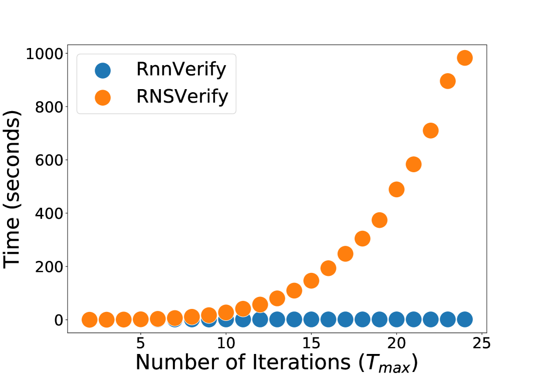
Figure 6: Average running time (in seconds) of RnnVerify and RNSVerify, as a function of $T_{\max}{}$.

Results. We began by comparing our technique to the state-of-the-art, unrolling-based RNSVerify tool [1], using the small network we had trained. Each dot in Fig. 6 represents a tool’s average run time on the 25 input points, for a specific $T_{\max}{}$. Both methods returned UNSAT on all queries; however, the runtimes clearly demonstrate that our approach is far less sensitive to large $T_{\max}{}$ values. In a separate experiment, our tool was able to solve a verification query on the same network with $T_{\max}{}=180$ in 2.5 seconds, whereas RNSVerify timed out after 24 hours.

Next, we used RnnVerify on all $2850$ benchmark queries on the 6 larger networks. The results appear in Sec. 11 of the appendix and are summarized as follows: (i) RnnVerify terminated on all benchmarks, with a median runtime of 5.39 seconds and an average runtime of $48.67$ seconds. The maximal solving time was 5701 seconds; (ii) $85\%$of RnnVerify’s runtime was spent within the underlying FFNN verification engine, solving $\varphi_{I}$ queries. This indicates that as the underlying FFNN verification technology improves, our approach will become significantly more scalable; (iii) for $1919$ ($67\%$) of the benchmarks, RnnVerify proved that the RNN was robust around the tested point. For the remaining $931$ benchmarks, the results are inconclusive: we do not know whether the network is vulnerable, or whether more sophisticated invariants are needed to prove robustness. This demonstrates that for a majority of tested benchmarks, the linear template proved useful; and (iv) RnnVerify could generally prove fewer instances with larger values of $T_{\max}$. This is because the linear bounds afforded by our invariants become more loose as $t$ increases, whereas the neuron’s values typically do not increase significantly over time. This highlights the need for more expressive invariants.

6 Related Work

Due to the discovery of undesirable behaviors in many DNNs, multiple approaches have been proposed for verifying them. These include the use of SMT solving [15, 17, 19, 23], LP and MILP solving [8, 32], symbolic interval propagation [34], abstract interpretation [9, 10], and many others (e.g., [2, 11, 14, 20, 25, 26]). Our technique focuses on RNN verification, but uses an FFNN verification engine as a back-end. Consequently, it could be integrated with many of the aforementioned tools, and will benefit from any improvement in scalability of FFNN verification technology.

Whereas FFNN verification has received a great deal of attention, only little research has been carried out on RNN verification. Akintunde et al. [1] were the first to propose such a technique, based on the notion of unrolling the network into an equivalent FFNN. Ko et al. [21] take a different approach, which aims at quantifying the robustness of an RNN to adversarial inputs — which can be regarded as an RNN verification technique tailored for a particular kind of properties. The scalability of both approaches is highly sensitive to the number of time steps, $T_{\max}{}$, specified by the property at hand. In this regard, the main advantage of our approach is that it is far less sensitive to the number of time steps being considered. This affords great potential for scalability, especially for long sequences of inputs. A drawback of our approach is that it requires invariant inference, which is known to be challenging.

In a very recent paper, Zhang et al. [37] propose a verification scheme aimed at RNNs that perform cognitive tasks. This scheme includes computing polytope invariants for the neuron layers of an RNN, using abstract interpretation and fixed-point analysis. We consider this as additional evidence of the usefulness of invariant generation in the context of RNN verification.

Automated invariant inference is a key problem in program analysis. A few notable methods for doing so include abstract-interpretation (e.g., [29]); counterexample-guided approaches (e.g., [27]); and learning-based approaches (e.g., [30]). It will be interesting to apply these techniques within the context of our framework, in order to more quickly and effectively discover useful invariants.

7 Conclusion

Neural network verification is becoming increasingly important to industry, regulators, and society as a whole. Research to date has focused primarily on FFNNs. We propose a novel approach for the verification of recurrent neural networks — a kind of neural networks that is particularly useful for context-dependent tasks, such as NLP. The cornerstone of our approach is the reduction of RNN verification to FFNN verification through the use of inductive invariants. Using a proof-of-concept implementation, we demonstrated that our approach can tackle many benchmarks orders-of-magnitude more efficiently than the state of the art. These experiments indicate the great potential that our approach holds. In the future, we plan to experiment with more expressive invariants, and also to apply compositional verification techniques in order to break the RNN into multiple, smaller networks, for which invariants can more easily be inferred.

Acknowledgements. This work was partially supported by the Semiconductor Research Corporation, the Binational Science Foundation (2017662), the Israel Science Foundation (683/18), and the National Science Foundation (1814369).

Appendix

8 Time-Dependent Properties

Our technique for verifying inferred invariants and for using them to solve the snapshot query (and hence to prove the property in question) hinges on our ability to reduce each step into an FFNN verification query. In order to facilitate this, we made the simplifying assumption that properties $P$ and $Q$ of the RNN verification query are time-agnostic; i.e. they are of the form $P=\bigwedge_{t=1}^{T_{\max}}\psi_{1}$ and $Q=\bigvee_{t=1}^{T_{\max}}\psi_{2}$ for $\psi_{1}$ and $\psi_{2}$ that are conjunctions of linear constraints. However, this limitation can be relaxed significantly.

Currently, input property $P$ specifies a constant range for the inputs, e.g. $-3\leq v_{1,1}^{t}\leq 3$ for all $1\leq t\leq T_{\max}{}$. However, we observe that our technique can be applied also for input properties that encode linear time constraints; e.g. $4t\leq v_{1,1}^{t}\leq 5t$. These properties can be transferred, as-is, to the FFNN snapshot network, and are compatible with our proposed technique. Likewise, the output property $Q$ can also include constraints that are linear in $t$; and can also restrict the query to a particular time step $t=t_{0}$. In fact, even more complex, piecewise-linear constraints can be encoded and are compatible with our technique. However, encoding these constraints might entail adding additional neurons to the RNN. For example, the constraint $(\max(v_{1,1}^{t},v_{1,2}^{t})\geq 5t)$ is piecewise-linear and can be encoded [3]; the encoding itself is technical, and is omitted. As for constraints that are not piecewise-linear, if these can be soundly approximated using piecewise-linear constraints, then they can be soundly handled using our technique.

9 Verification Algorithm for RNNs with Multiple Memory Units in Separate Layers

As described in Sec. 4.1, we take an iterative approach to verify networks with multiple memory units, each in a separate layer. We start from the input layer and prove an invariant for each layer that has memory units; and when proving an invariant for layer $i+1$, we use the already-proven invariants of layers $1$ through $i$.

An example appears in Fig. 7. Let $P=\bigwedge_{t=1}^{5}(-3\leq v^{t}_{1,1}\leq 3)$ and $Q=\bigvee_{t=1}^{5}(v_{4,1}^{t}\geq 60)$. First we construct the snapshot network shown in the figure. Next, we prove the invariant $v_{2,1}^{m}\leq 3(t-1)$, same as we did before. This invariant bounds the values of $v_{2,1}^{m}$. Next, we use this information in proving an invariant also for $v_{3,1}$; e.g., $v_{3,1}^{m}\leq 9\cdot(t-1)$. To see why this is an invariant, observe that

$$v_{3,1}^{t}\leq\sum_{i=1}^{t}v_{2,1}^{i}\stackrel{{\scriptstyle*}}{{\leq}}\sum_{i=1}^{t}3i=(3+3t)\frac{t}{2}\leq(3+3T_{\max})\frac{t}{2}=9t$$

Note that the invariant for $v_{2,1}$ was used in the $*$ transition. Once this second invariant is proved, we can show that the original property holds, by using FFNN verification to show that $\langle P,\mathcal{S}(N),v_{4,1}\geq 60\rangle$ is UNSAT; where $\mathcal{S}(N)$ is the FFNN from Fig. 7, and

$$P=(-3\leq v_{1,1}\leq 3)\wedge(1\leq t\leq 5)\wedge(v_{2,1}^{m}\leq 3(t-1))\wedge(v_{3,1}^{m}\leq 9(t-1))$$

(a) Original Netowrk

(b) Snapshot network

Figure 7: An RNN with multiple memory units, in separate layers (on the left), and its snapshot network (on the right).

Algorithm 2 describe the complete process. We assume for simplicity that every hidden layer in the RNN has a (single) memory unit. Initially (Lines 2-5), the algorithm guesses and verifies a very coarse upper bound on each of the memory units. Next, it repeatedly attempts to solve the snapshot query $\hat{\varphi}$ using the current invariants. If successful, we are done (Line 9); and otherwise, we start another pass over the network’s layers, attempting to strengthen each invariant in turn. We know we have reached an optimal invariant for a layer when the search range for that layer’s $\alpha$ becomes smaller than some small $\epsilon$ constant (Line 13). The algorithm fails (Line 22) when (i) optimal invariants for all layers have been discovered; and (ii) these optimal invariants are insufficient for solving the snapshot query. For simplicity, the algorithm only deals with upper bounds, but it can be extended to incorporate lower bound invariants as well in a straightforward manner.

Algorithm 2 Automatic Multiple Memory Units Verification($P,N,Q,T_{\max}$)

1:Construct the snapshot network $\hat{N}$

2:for $i=2$ to $n-1$ do

3:     $lb_{i}\leftarrow-M\cdot i,ub_{i}\leftarrow M\cdot i,\alpha_{i}\leftarrow M\cdot i$ COMMENT$\triangleright$ M is a large constant

4:     $I_{i}\leftarrow v_{i}^{m}\leq\alpha_{i}\cdot t$ COMMENT$\triangleright$ Loose invariant, should hold

5:     if $\varphi_{I_{i}}$ is SAT then return False COMMENT$\triangleright$ Loose invariant fails, give up      

6:while True do

7:     Construct $\hat{\varphi}$ using the invariant $\bigwedge_{i=2}^{n-1}I_{i}$

8:     if $\hat{\varphi}$ is UNSAT then

9:         return True COMMENT$\triangleright$ Invariants sufficiently strong

10:     else

11:         progressMade $\leftarrow$ False

12:         for $i=2$ to $n-1$ do

13:              if $ub_{i}-lb_{i}\leq\epsilon$ then

14:                  Continue COMMENT$\triangleright$ Already have optimal invariant               

15:              progressMade $\leftarrow$ True COMMENT$\triangleright$ Still searching for optimal invariant

16:              $\alpha_{i}^{\prime}\leftarrow(ub_{i}+lb_{i})/2$

17:              $I_{i}^{\prime}\leftarrow v_{i}^{m}\leq\alpha_{i}^{\prime}\cdot t$

18:              if $\varphi_{I_{i}}^{\prime}$ is UNSAT then

19:                  $I_{i}\leftarrow I_{i}^{\prime},\alpha_{i}\leftarrow\alpha_{i}^{\prime},ub_{i}\leftarrow\alpha_{i}$ COMMENT$\triangleright$ Better invariant found

20:              else

21:                  $lb_{i}\leftarrow\alpha_{i}^{\prime}$ COMMENT$\triangleright$ Invariant unchanged, range shrinks                        

22:         if !progressMade then return False COMMENT$\triangleright$ Best invariants too weak               

A key property of our layer-by-layer approach for invariant inference is that accurate invariants for layer $i$ are crucial for proving invariants for layer $i+1$. When each layer contains a single neuron, finding the optimal invariant for each layer is straightforward; but, as we discuss in Sec. 4.2, things are not as simple when multiple memory units reside in the same layer.

10 Invariant Inference without MILP

In cases where using an MILP solver is undesirable (for example, if $T_{\max}$ is very large and the MILP instances become a bottleneck), we propose an incremental approach. Here, we start with an arbitrary assignment of $\alpha$ values, which may or may not constitute an invariant, and iteratively change one $\alpha$ at a time. This change needs to be “in the right direction” — i.e., if our $\alpha$’s do not currently constitute an invariant, we need to weaken the bounds; and if they do constitute an invariant but that invariant is too weak to solve $\hat{\varphi}$, we need to tighten the bounds. The selection of which $\alpha$ to change and by how much to change it can be random, arbitrary, or according to some heuristic. In our experiments we observed that while this approach is computationally cheaper than solving MILP instances, it tends to lead to longer sequences of refining the $\alpha$’s before an appropriate invariant is found. Devising heuristics that will improve the efficiency of this approach remains a topic for future work.

11 Experimental Results

Table 1 fully describes the result of running RnnVerify on all $2850$ benchmark queries that we used. Network $N_{x,y}$ has a hidden layer with $x$ memory units; a second hidden layer with $y$ memory units, if $y>0$; and $5$ fully connected layers, each with $32$ nodes. All experiments were run using using an Intel Xeon E5 machine with $6$ cores and $3$GB of memory. Each entry depicts the average runtime, in seconds, over the 25 input points; and also the number $x/25$ of queries where RnnVerify successfully proved adversarial robustness. In the remaining $25-x$ queries, linear invariants were insufficient for proving that the snapshot query is UNSAT. The results are generally monotonic: as $T_{\max}{}$ increases, fewer instances can be verified. We used $\dagger$ to mark the few cases where monotonicity was broken. Our inspection revealed that these cases were due to numerical instability that occurred in either the underlying MILP solver or the FFNN verification tools.

Table 1: Running RnnVerify on our $2850$ benchmarks.

$T_{\max}{}$			$N_{2,0}$			$N_{2,2}$			$N_{4,0}$			$N_{4,2}$			$N_{4,4}$			$N_{8,0}$
2			0.21(25/25)			0.69(25/25)			0.56(25/25)			0.60(25/25)			1.13(25/25)			1.80(25/25)
3			4.00(25/25)			21.72(25/25)			17.06(25/25)			39.05(25/25)			21.42(25/25)			28.82(5/25)
4			4.94(25/25)			28.54(25/25)			27.52(25/25)			80.18(23/25)			42.04(25/25)			9.08(2/25)
5			5.57(25/25)			30.01(25/25)			24.22(25/25)			48.97(19/25)			11.61(25/25)			12.61(2/25)
6			6.01(25/25)			22.92(25/25)			57.14(24/25)†			78.09(17/25)			4.80(25/25)			18.01(2/25)
7			6.39(25/25)			31.43(25/25)			61.79(25/25)			68.70(17/25)			3.03(9/25)			19.43(2/25)
8			6.64(25/25)			7.80(25/25)			47.60(25/25)			98.05(15/25)†			3.07(8/25)†			27.65(2/25)
9			7.05(25/25)			8.66(25/25)			85.26(23/25)			147.65(16/25)			3.73(9/25)			26.49(2/25)
10			7.06(25/25)			10.72(25/25)			82.29(14/25)			239.96(16/25)			3.99(8/25)†			33.12(2/25)
11			7.38(25/25)			13.38(25/25)			122.94(14/25)			150.03(16/25)			4.71(8/25)†			29.59(2/25)
12			7.46(25/25)			10.28(25/25)			107.15(14/25)			15.75(16/25)			4.33(8/25)†			47.05(2/25)
13			14.61(25/25)			10.61(25/25)			218.79(13/25)			16.93(16/25)			4.87(9/25)			43.38(2/25)
14			7.95(25/25)			11.41(25/25)			149.37(12/25)			18.08(16/25)			5.41(8/25)			44.16(2/25)
15			14.50(25/25)			11.99(25/25)			365.37(12/25)			19.56(16/25)			6.12(8/25)			52.22(2/25)
16			8.24(25/25)			12.56(25/25)			294.83(12/25)			20.71(16/25)			6.67(8/25)			55.62(2/25)
17			8.30(25/25)			13.30(25/25)			323.97(12/25)			20.90(15/25)			6.65(8/25)			66.14(2/25)
18			8.35(25/25)			13.93(25/25)			481.18(12/25)			21.68(15/25)			7.71(8/25)			82.93(2/25)
19			8.56(25/25)			14.46(25/25)			350.61(12/25)			23.36(15/25)			7.85(8/25)			75.68(2/25)
20			8.61(25/25)			15.17(25/25)			264.39(12/25)			24.28(15/25)			8.24(8/25)			71.26(2/25)

References

- [1] M. Akintunde, A. Kevorchian, A. Lomuscio, and E. Pirovano. Verification of RNN-Based Neural Agent-Environment Systems. In Proc. 33rd Conf. on Artificial Intelligence (AAAI), pages 6006–6013, 2019.
- [2] R. Bunel, I. Turkaslan, P. Torr, P. Kohli, and P. Mudigonda. A Unified View of Piecewise Linear Neural Network Verification. In Proc. 32nd Conf. on Neural Information Processing Systems (NeurIPS), pages 4795–4804, 2018.
- [3] N. Carlini, G. Katz, C. Barrett, and D. Dill. Provably Minimally-Distorted Adversarial Examples, 2017. Technical Report. https://arxiv.org/abs/1709.10207.
- [4] C.-H. Cheng, G. Nührenberg, C.-H. Huang, and H. Ruess. Verification of Binarized Neural Networks via Inter-Neuron Factoring. In Proc. 10th Working Conf. on Verified Software: Theories, Tools, and Experiments (VSTTE), pages 279–290, 2018.
- [5] C.-H. Cheng, G. Nührenberg, and H. Ruess. Maximum Resilience of Artificial Neural Networks. In Proc. 15th Int. Symp. on Automated Technology for Verification and Analysis (ATVA), pages 251–268, 2017.
- [6] M. Cisse, Y. Adi, N. Neverova, and J. Keshet. Houdini: Fooling Deep Structured Visual and Speech Recognition Models with Adversarial Examples. In Proc. 30th Advances in Neural Information Processing Systems (NIPS), pages 6977–6987, 2017.
- [7] J. Devlin, M. Chang, K. Lee, and K. Toutanova. BERT: Pre-training of Deep Bidirectional Transformers for Language Understanding, 2018. Technical Report. http://arxiv.org/abs/1810.04805.
- [8] R. Ehlers. Formal Verification of Piece-Wise Linear Feed-Forward Neural Networks. In Proc. 15th Int. Symp. on Automated Technology for Verification and Analysis (ATVA), pages 269–286, 2017.
- [9] Y. Elboher, J. Gottschlich, and G. Katz. An Abstraction-Based Framework for Neural Network Verification. In Proc. 32nd Int. Conf. on Computer Aided Verification (CAV), 2020.
- [10] T. Gehr, M. Mirman, D. Drachsler-Cohen, E. Tsankov, S. Chaudhuri, and M. Vechev. AI2: Safety and Robustness Certification of Neural Networks with Abstract Interpretation. In Proc. 39th IEEE Symposium on Security and Privacy (S&P), 2018.
- [11] S. Gokulanathan, A. Feldsher, A. Malca, C. Barrett, and G. Katz. Simplifying Neural Networks using Formal Verification. In Proc. 12th NASA Formal Methods Symposium (NFM), 2020.
- [12] B. Goldberger, Y. Adi, J. Keshet, and G. Katz. Minimal Modifications of Deep Neural Networks using Verification. In Proc. 23rd Int. Conf. on Logic for Programming, Artificial Intelligence and Reasoning (LPAR), pages 260–278, 2020.
- [13] I. Goodfellow, Y. Bengio, and A. Courville. Deep Learning. MIT Press, 2016.
- [14] D. Gopinath, G. Katz, C. Pǎsǎreanu, and C. Barrett. DeepSafe: A Data-driven Approach for Assessing Robustness of Neural Networks. In Proc. 16th. Int. Symposium on on Automated Technology for Verification and Analysis (ATVA), pages 3–19, 2018.
- [15] X. Huang, M. Kwiatkowska, S. Wang, and M. Wu. Safety Verification of Deep Neural Networks. In Proc. 29th Int. Conf. on Computer Aided Verification (CAV), pages 3–29, 2017.
- [16] Y. Jacoby, C. Barrett, and G. Katz. RnnVerify, 2020. https://github.com/yuvaljacoby/RnnVerify.
- [17] G. Katz, C. Barrett, D. Dill, K. Julian, and M. Kochenderfer. Reluplex: An Efficient SMT Solver for Verifying Deep Neural Networks. In Proc. 29th Int. Conf. on Computer Aided Verification (CAV), pages 97–117, 2017.
- [18] G. Katz, C. Barrett, D. Dill, K. Julian, and M. Kochenderfer. Towards Proving the Adversarial Robustness of Deep Neural Networks. In Proc. 1st Workshop on Formal Verification of Autonomous Vehicles, (FVAV), pages 19–26, 2017.
- [19] G. Katz, D. Huang, D. Ibeling, K. Julian, C. Lazarus, R. Lim, P. Shah, S. Thakoor, H. Wu, A. Zeljić, D. Dill, M. Kochenderfer, and C. Barrett. The Marabou Framework for Verification and Analysis of Deep Neural Networks. In Proc. 31st Int. Conf. on Computer Aided Verification (CAV), pages 443–452, 2019.
- [20] Y. Kazak, C. Barrett, G. Katz, and M. Schapira. Verifying Deep-RL-Driven Systems. In Proc. 1st ACM SIGCOMM Workshop on Network Meets AI & ML (NetAI), pages 83–89, 2019.
- [21] C. Ko, Z. Lyu, T. Weng, L. Daniel, N. Wong, and D. Lin. POPQORN: Quantifying Robustness of Recurrent Neural Networks. In Proc. 36th IEEE Int. Conf. on Machine Learning and Applications (ICML), 2019.
- [22] F. Kreuk, Y. Adi, M. Cisse, and J. Keshet. Fooling End-to-End Speaker Verification with Adversarial Examples. In Proc. IEEE Int. Conf. on Acoustics, Speech and Signal Processing (ICASSP), pages 1962–1966, 2018.
- [23] L. Kuper, G. Katz, J. Gottschlich, K. Julian, C. Barrett, and M. Kochenderfer. Toward Scalable Verification for Safety-Critical Deep Networks, 2018. Technical Report. https://arxiv.org/abs/1801.05950.
- [24] Z. Lipton, D. Kale, C. Elkan, and R. Wetzel. Learning to Diagnose with LSTM Recurrent Neural Networks. In Proc. 4th Int. Conf. on Learning Representations (ICLR), 2016.
- [25] A. Lomuscio and L. Maganti. An Approach to Reachability Analysis for Feed-Forward ReLU Neural Networks, 2017. Technical Report. http://arxiv.org/abs/1706.07351.
- [26] N. Narodytska, S. Kasiviswanathan, L. Ryzhyk, M. Sagiv, and T. Walsh. Verifying Properties of Binarized Deep Neural Networks, 2017. Technical Report. http://arxiv.org/abs/1709.06662.
- [27] T. Nguyen, T. Antonopoulos, A. Ruef, and M. Hicks. Counterexample-Guided Approach to Finding Numerical Invariants. In Proc. 11th Joint Meeting on Foundations of Software Engineering (FSE), pages 605–615, 2017.
- [28] O. Padon, N. Immerman, S. Shoham, A. Karbyshev, and M. Sagiv. Decidability of Inferring Inductive Invariants. In Proc. 43th Symposium on Principles of Programming Languages (POPL), pages 217–231, 2016.
- [29] R. Sharma, I. Dillig, T. Dillig, and A. Aiken. Simplifying Loop Invariant Generation Using Splitter Predicates. In Proc. 23rd Int. Conf. on Computer Aided Verification (CAV), pages 703–719, 2011.
- [30] X. Si, H. Dai, M. Raghothaman, M. Naik, and L. Song. Learning Loop Invariants for Program Verification. In Proc. 32nd Conf. on Neural Information Processing Systems (NeurIPS), pages 7762–7773, 2018.
- [31] C. Szegedy, W. Zaremba, I. Sutskever, J. Bruna, D. Erhan, I. Goodfellow, and R. Fergus. Intriguing Properties of Neural Networks, 2013. Technical Report. http://arxiv.org/abs/1312.6199.
- [32] V. Tjeng, K. Xiao, and R. Tedrake. Evaluating Robustness of Neural Networks with Mixed Integer Programming. In Proc. 7th Int. Conf. on Learning Representations (ICLR), 2019.
- [33] L. Wan, Q. Wang, A. Papir, and I. Lopez-Moreno. Generalized End-to-End Loss for Speaker Verification, 2017. Technical Report. http://arxiv.org/abs/1710.10467.
- [34] S. Wang, K. Pei, J. Whitehouse, J. Yang, and S. Jana. Formal Security Analysis of Neural Networks using Symbolic Intervals. In Proc. 27th USENIX Security Symposium, pages 1599–1614, 2018.
- [35] H. Wu, A. Ozdemir, A. Zeljić, A. Irfan, K. Julian, D. Gopinath, S. Fouladi, G. Katz, C. Păsăreanu, and C. Barrett. Parallelization Techniques for Verifying Neural Networks, 2020. Technical Report. https://arxiv.org/abs/2004.08440.
- [36] J. Yamagishi, C. Veaux, and K. MacDonald. CSTR VCTK Corpus: English Multi-speaker Corpus for CSTR Voice Cloning Toolkit, 2019. University of Edinburgh. https://doi.org/10.7488/ds/2645.
- [37] H. Zhang, M. Shinn, A. Gupta, A. Gurfinkel, N. Le, and N. Narodytska. Verification of Recurrent Neural Networks for Cognitive Tasks via Reachability Analysis. In Proc. 24th Conf. of European Conference on Artificial Intelligence (ECAI), 2020.