A Count Sketch Kaczmarz Method For Solving Large Overdetermined Linear Systems

Abstract

In this paper, combining count sketch and maximal weighted residual Kaczmarz method, we propose a fast randomized algorithm for large overdetermined linear systems. Convergence analysis of the new algorithm is provided. Numerical experiments show that, for the same accuracy, our method behaves better in computing time compared with the state-of-the-art algorithm.

1 Introduction

We consider the following consistent linear systems

$$Ax=b,$$ (1)

where $A\in R^{m\times n}$ with $m\gg n$, $b\in R^{m}$, and $x$ is the $n$-dimensional unknown vector. As we know, the Kaczmarz method [1] is a popular so-called row-action method for solving the systems (1). In 2009, Strohmer and Vershynin [2] proved the linear convergence of the randomized Kaczmarz (RK) method. Latter, many Kaczmarz type methods were proposed for different possible systems settings; see for example [3, 4, 5, 6, 7, 8, 9, 10] and references therein.

Recently, Bai and Wu [11] constructed a greedy randomized Kaczmarz (GRK) method by introducing an efficient probability criterion for selecting the working rows from the coefficient matrix, which avoids a weakness of the one adopted in the RK method. Based on GRK method, a so-called relaxed greedy randomized Kaczmarz (RGRK) method was proposed in [12] by introducing a relaxation parameter, which makes the convergence factor of RGRK method be smaller than that of GRK method when the relaxation parameter $\theta\in[\frac{1}{2},1]$, and the convergence factor reaches the minimum when $\theta=1$. For the latter case, i.e., $\theta=1$, Du and Gao [13] called it the maximal weighted residual Kaczmarz (MWRK) method and carried out extensive experiments to test this method.

In this paper, inspired by dimensionality reduction techniques [14], we propose a count sketch Kaczmarz (CSK) method by combining count sketch [15, 16] and MWRK method. The convergence of CSK method is proved. Numerical experiments show that our method outperforms MWRK method in computing time.

The rest of this paper is organized as follows. In Section 2, some notations and the definition of count sketch are first given. Then, the CSK method is presented and its convergence is analyzed. Numerical experiments are given in Section 3.

2 The CSK method

Throughout the paper, for a matrix $A$, $A^{(i)}$, $A_{(j)}$, $\sigma_{i}(A)$, $\sigma_{r}(A)$, $\|A\|_{F}$ and ${\rm R(A)}$ denote its $i$th row (or $i$th entry in the case of a vector), $j$th column, $i$th singular value, smallest nonzero singular value, Frobenius norm, and column space, respectively.

We now list the definition of count sketch which can be found in [15, 16].

Definition 1

(Count Sketch transform). A count sketch transform is defined to be $\mathbf{S}=\Phi D\in{R^{d\times m}}$. Here, $D$ is an $m\times m$ random diagonal matrix with each diagonal entry independently chosen to be $+1$ or $-1$ with equal probability, and $\Phi\in\{0,1\}^{d\times m}$ is a $d\times m$ binary matrix with $\Phi_{h(i),i}=1$ and all remaining entries 0, where $h:[m]\rightarrow[d]$ is a random map such that for each $i\in[m]$, $h(i)=j$ with probability $1/d$ for each $j\in[d]$.

Next, we give our new method.

Algorithm 1

The CSK method for the solution of the linear systems (1)

1. INPUT:   Matrix $A\in R^{m\times n}$, vector $b\in R^{m}$, parameter $d$, initial estimate $x_{0}$

2. OUTPUT:  Approximate $x$ solving $Ax=b$

3. Initialize:  Create a count sketch $\mathbf{S}\in{R^{d\times m}}$ with $d<m$, and compute $\widetilde{A}=\mathbf{S}A$ and $\widetilde{b}=\mathbf{S}b$.

4. For $k=0,1,2,\ldots,$ do until satisfy the stopping criteria

5. Compute $i_{k}={\rm arg}\max\limits_{1\leq i\leq d}\{\frac{|\widetilde{b}^{(i)}-\widetilde{A}^{(i)}x_{k}|}{\|\widetilde{A}^{(i)}\|_{2}}\}$.

6. Set $x_{k+1}=x_{k}+\frac{\widetilde{b}^{(i_{k})}-\widetilde{A}^{(i_{k})}x_{k}}{\|\widetilde{A}^{(i_{k})}\|_{2}^{2}}(\widetilde{A}^{(i_{k})})^{T}$.

7. End for

Remark 1

In MWRK method, the selection strategy for index is $i_{k}=\arg\max\limits_{1\leq i\leq m}\{\frac{|b^{(i)}-A^{(i)}x_{k}|}{\|A^{(i)}\|_{2}}\}$. So, the difference between Algorithm 1 and MWRK method is that we introduce the count sketch transform $\mathbf{S}$. From [14] and [17], we know that S can reduce the computation cost with keeping the most of the information of original problem. So, our method will behave better in runtime and a little worse in accuracy, which are conformed by numerical experiments given in Section 3.

In the following, we provide theoretical guarantees for the convergence of the CSK method. A lemma is first given as follows, which plays a fundamental role in the convergence analysis.

Lemma 1

([14]) If $\mathbf{S}$ is a count sketch transform with $O(n^{2}/(\delta\varepsilon^{2}))$ rows, where $0<\delta,\varepsilon<1$, then we have that

$$(1-\varepsilon)\|Ax\|^{2}_{2}\leq\|\mathbf{S}Ax\|^{2}_{2}\leq(1+\varepsilon)\|Ax\|^{2}_{2}~{}for~{}all~{}x\in R^{n},$$ (2)

and

$$(1-\varepsilon)\sigma_{i}(\textbf{S}A)\leq\sigma_{i}(A)\leq(1+\varepsilon)\sigma_{i}(\textbf{S}A)~{}for~{}all~{}1\leq i\leq n$$ (3)

hold with probability $1-\delta$.

Theorem 2

Let $\mathbf{S}\in{R^{d\times m}}$ be a count sketch transform with $d=O(n^{2}/(\delta\varepsilon^{2}))$ and $x_{\star}=A^{\dagger}b$ be the solution of the systems (1). From an initial guess $x_{0}\in R^{n}$ in the column space of $A^{T}$, for the sequence $\{x_{k}\}_{k=0}^{\infty}$ generated by the CSK method, we have that

$$\|x_{k+1}-x_{\star}\|^{2}_{2}\leq\left(1-\frac{(1-\varepsilon)^{3}}{n}\cdot\frac{\sigma^{2}_{r}(A)}{\|A\|^{2}_{2}}\right)\|x_{k}-x_{\star}\|^{2}_{2}$$

holds with probability at least $1-2\delta$.

Proof 1

From Algorithm 1, using the fact $Ax_{\star}=b$, we have

$$x_{k+1}-x_{\star} = x_{k}-x_{\star}+\frac{\widetilde{b}^{(i_{k})}-\widetilde{A}^{(i_{k})}x_{k}}{\|\widetilde{A}^{(i_{k})}\|_{2}^{2}}(\widetilde{A}^{(i_{k})})^{T}$$

$$= x_{k}-x_{\star}+\frac{\mathbf{S}^{(i_{k})}b-\mathbf{S}^{(i_{k})}Ax_{k}}{\|\mathbf{S}^{(i_{k})}A\|_{2}^{2}}(\mathbf{S}^{(i_{k})}A)^{T}$$

$$= \left(I-\frac{(\mathbf{S}^{(i_{k})}A)^{T}\mathbf{S}^{(i_{k})}A}{\|\mathbf{S}^{(i_{k})}A\|_{2}^{2}}\right)(x_{k}-x_{\star}).$$

Taking the square of the Euclidean norm on both sides and applying some algebra, we get

$$\|x_{k+1}-x_{\star}\|^{2}_{2} =\left\|\left(I-\frac{(\mathbf{S}^{(i_{k})}A)^{T}\mathbf{S}^{(i_{k})}A}{\|\mathbf{S}^{(i_{k})}A\|_{2}^{2}}\right)(x_{k}-x_{\star})\right\|^{2}_{2}$$

$$=(x_{k}-x_{\star})^{T}\left(I-\frac{(\mathbf{S}^{(i_{k})}A)^{T}\mathbf{S}^{(i_{k})}A}{\|\mathbf{S}^{(i_{k})}A\|_{2}^{2}}\right)(x_{k}-x_{\star})$$

$$=\|x_{k}-x_{\star}\|^{2}_{2}-\frac{|\mathbf{S}^{(i_{k})}A(x_{k}-x_{\star})|^{2}}{\|\mathbf{S}^{(i_{k})}A\|_{2}^{2}}.$$ (4)

Note that, from Algorithm 1,

$$i_{k} = {\rm arg}\max\limits_{1\leq i\leq d}\{\frac{|\widetilde{b}^{(i)}-\widetilde{A}^{(i)}x_{k}|}{\|\widetilde{A}^{(i)}\|_{2}}\}={\rm arg}\max\limits_{1\leq i\leq d}\frac{|\textbf{S}^{(i)}b-\textbf{S}^{(i)}Ax_{k}|^{2}}{\|\textbf{S}^{(i)}A\|^{2}_{2}}$$

$$= {\rm arg}\max\limits_{1\leq i\leq d}\frac{|\mathbf{S}^{(i)}A(x_{k}-x_{\star})|^{2}}{\|\mathbf{S}^{(i)}A\|_{2}^{2}}.$$

Then

$$\frac{|\mathbf{S}^{(i_{k})}A(x_{k}-x_{\star})|^{2}}{\|\mathbf{S}^{(i_{k})}A\|_{2}^{2}} =\max\limits_{1\leq i\leq d}\frac{|\mathbf{S}^{(i)}A(x_{k}-x_{\star})|^{2}}{\|\mathbf{S}^{(i)}A\|_{2}^{2}}\geq\sum_{i=1}^{d}\frac{\|\mathbf{S}^{(i)}A\|^{2}_{2}}{\|\mathbf{S}A\|^{2}_{F}}\frac{|\mathbf{S}^{(i)}A(x_{k}-x_{\star})|^{2}}{\|\mathbf{S}^{(i)}A\|_{2}^{2}}$$

$$=\frac{\|\mathbf{S}A(x_{k}-x_{\star})\|^{2}_{2}}{\|\mathbf{S}A\|^{2}_{F}}.$$ (5)

Substituting (5) into (4), we obtain

$$\|x_{k+1}-x_{\star}\|^{2}_{2} \leq\|x_{k}-x_{\star}\|^{2}_{2}-\frac{\|\mathbf{S}A(x_{k}-x_{\star})\|^{2}_{2}}{\|\mathbf{S}A\|^{2}_{F}}\leq\|x_{k}-x_{\star}\|^{2}_{2}-\frac{\|\mathbf{S}A(x_{k}-x_{\star})\|^{2}_{2}}{n\|\mathbf{S}A\|^{2}_{2}},$$ (6)

where the last inequality follows from the inequality $\|\mathbf{S}A\|^{2}_{F}\leq n\|\mathbf{S}A\|^{2}_{2}$.

As explained in [11], since $x_{\star}=A^{\dagger}b\in{\rm R(A^{T})}$, by starting from an arbitrary initial guess $x_{0}$ in the column space of $A^{T}$, we have from the algorithm that $x_{k}$ also doe for each $k$ and hence, $x_{k}-x_{\star}$ is in the column space of $A^{T}$, which indicates that

$$\|A(x_{k}-x_{\star})\|^{2}_{2}\geq\sigma^{2}_{r}(A)\|x_{k}-x_{\star}\|^{2}_{2}.$$

Exploiting the above inequality and (2), with probability $1-\delta$, we have

$$\|\mathbf{S}A(x_{k}-x_{\star})\|^{2}_{2} \geq(1-\varepsilon)\|A(x_{k}-x_{\star})\|^{2}_{2}\geq(1-\varepsilon)\sigma^{2}_{r}(A)\|x_{k}-x_{\star}\|^{2}_{2}.$$ (7)

Meanwhile, by (3), with probability $1-\delta$, we have

$$(1-\varepsilon)\sigma_{1}(\textbf{S}A) \leq \sigma_{1}(A).$$

That is, with probability $1-\delta$, we have

$$\|\textbf{S}A\|^{2}_{2} \leq\frac{1}{(1-\varepsilon)^{2}}\|A\|^{2}_{2}.$$ (8)

Thus, combining (7) and (8), with probability at least $1-2\delta$, we get

$$\frac{\|\mathbf{S}A(x_{k}-x_{\star})\|^{2}_{2}}{\|\textbf{S}A\|^{2}_{2}} \geq(1-\varepsilon)^{3}\cdot\frac{\sigma^{2}_{r}(A)\|x_{k}-x_{\star}\|^{2}_{2}}{\|A\|^{2}_{2}}.$$ (9)

Substituting (9) into (6), with probability at least $1-2\delta$, we have

$$\|x_{k+1}-x_{\star}\|^{2}_{2} \leq \|x_{k}-x_{\star}\|^{2}_{2}-\frac{(1-\varepsilon)^{3}}{n}\cdot\frac{\sigma^{2}_{r}(A)\|x_{k}-x_{\star}\|^{2}_{2}}{\|A\|^{2}_{2}},$$

which implies the desired result.

Remark 2

Note that $(1-\frac{(1-\varepsilon)^{3}}{n}\cdot\frac{\sigma^{2}_{r}(A)}{\|A\|^{2}_{2}})<(1-\frac{\sigma^{2}_{r}(A)}{\max\limits_{1\leq i\leq m}\sum\limits^{m}_{j=1,j\neq i}\|A^{(j)}\|^{2}_{2}})$, where the latter is the convergence factor of MWRK method. So the convergence factor of CSK method is a little lager. This is because introducing count sketch transform $\mathbf{S}$ produces additional errors for algorithm.

3 Numerical experiments

In this section, we mainly compare the CSK method and the MWRK method in terms of the iteration numbers (denoted as “IT”) and computing time in seconds (denoted as “CPU”). We also report the iteration number speedup of CSK against MWRK, which is defined as

$$\texttt{IT speedup}=\frac{\texttt{IT of }\texttt{MWRK}}{\texttt{IT of }\texttt{CSK}},$$

and the computing time speedup of CSK against MWRK, which is defined as

$$\texttt{CPU speedup}=\frac{\texttt{CPU of }\texttt{MWRK}}{\texttt{CPU of }\texttt{CSK}}.$$

In all the following specific experiments, we generate the coefficient matrix $A\in R^{m\times n}$ and the solution vector $x_{\star}\in R^{n}$ using the MATLAB function randn, and the vector $b\in R^{m}$ by setting $b=Ax_{\star}$ and set $d=n^{2}$. We repeat 50 experiments and all the experiments start from an initial vector $x_{0}=0$, and terminate once the relative solution error (RES), defined by

$$\rm RES=\frac{\left\|x_{k}-x_{\star}\right\|^{2}_{2}}{\left\|x_{\star}\right\|^{2}_{2}},$$

satisfies $\rm RES\leq 10^{-6}$, or the number of iteration steps exceeds 20000.

Table 1: Numerical results for the CSK and MWRK methods.

$m\times n$	IT			CPU
	CSK	MWRK	IT speedup	CSK	MWRK	CPU speedup
$300000\times 50$	54.9000	31.0000	0.5647	0.2209	1.6878	7.6393
$300000\times 100$	94.8600	63.0000	0.6641	0.4569	5.1097	11.1840
$300000\times 150$	132.7600	96.0000	0.7231	1.4894	10.3728	6.9645
$400000\times 50$	54.3600	29.0000	0.5335	0.2597	1.9737	7.6005
$400000\times 100$	95.1400	60.0000	0.6306	0.5778	6.0903	10.5403
$400000\times 150$	132.5600	94.0000	0.7091	1.8509	13.1016	7.0783
$500000\times 50$	55.1000	29.0000	0.5263	0.3312	2.5878	7.8123
$500000\times 100$	94.9600	60.0000	0.6318	0.7366	8.2903	11.2554
$500000\times 150$	132.5400	91.0000	0.6866	2.0513	17.3091	8.4383
$600000\times 50$	54.8800	28.0000	0.5102	0.4053	3.1672	7.8142
$600000\times 100$	95.1600	58.0000	0.6095	0.8566	10.2019	11.9103
$600000\times 150$	132.5800	92.0000	0.6939	2.3828	22.0388	9.2490
$700000\times 50$	54.7000	29.0000	0.5302	0.4550	3.9312	8.6401
$700000\times 100$	95.4200	58.0000	0.6078	1.0025	12.2144	12.1839
$700000\times 150$	132.3600	89.0000	0.6724	2.7194	25.7228	9.4591

The numerical results on IT and CPU are listed in Table 1. Here, it should be pointed out that the IT and CPU in Table 1 denote the means of IT and CPU of 50 tests. From Table 1, we see that the CSK method requires more iterations compared with the MWRK method. This is because the CSK method has larger convergence factor and hence converges a little slower, which is consistent with the analysis of Remarks 2 and 1. However, the runtime of the CSK method is less than that of the MWRK method, and the CPU speedup can be as large as 12.1839 in our experiments, which is consistent with the analysis of Remark 1.

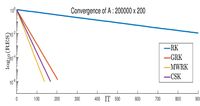
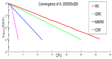
Figure 1: ${\rm log_{10}(RES)}$ versus IT (left) and CPU (right) for RK, GRK, MWRK, and CSK when $A\in R^{200000\times 200}$.

We also compare the performance of four algorithms (RK, GRK, MWRK, CSK). In Figure 1, we plot the RES in base-10 logarithm versus the IT and CPU of four algorithms for $A\in R^{200000\times 200}$. Each line represents the median RES at that iteration or CPU time over 50 trials. From the figure, we find that the CSK and MWRK methods outperform the RK and GRK methods in terms of IT and CPU, the MWRK method converges fastest, and the CSK method needs the least runtime for the same accuracy.

References

- [1] S. Kaczmarz, Angenäherte auflösung von systemen linearer gleichungen, Bull. Int. Acad. Pol. Sci. Lett. A 35 (1937) 355–357.
- [2] T. Strohmer, R. Vershynin, A randomized Kaczmarz algorithm with exponential convergence, J. Fourier Anal. Appl. 15 (2009) 262–278.
- [3] D. Needell, Randomized Kaczmarz solver for noisy linear systems, BIT Numer. Math. 50 (2010) 395–403.
- [4] Y. Eldar, D. Needell, Acceleration of randomized Kaczmarz method via the Johnson-Lindenstrauss lemma, Numer. Algor. 58 (2011) 163–177.
- [5] A. Zouzias, M. N. Freris, Randomized extended Kaczmarz for solving least squares, SIAM J. Matrix Anal. Appl. 34 (2013) 773–793.
- [6] A. Ma, D. Needell, A. Ramdas, Convergence properties of the randomized extended gauss-seidel and Kaczmarz methods, SIAM J. Matrix Anal. Appl. 36 (2015) 1590–1604.
- [7] Y. Liu, C. Q. Gu, Variant of greedy randomized Kaczmarz for ridge regression, Appl. Numer. Math. 143 (2019) 223–246.
- [8] K. Du, Tight upper bounds for the convergence of the randomized extended Kaczmarz and Gauss–Seidel algorithms, Numer. Linear Algebra Appl. 26 (3) (2019) e2233.
- [9] N. C. Wu, H. Xiang, Projected randomized Kaczmarz methods, J. Comput. Appl. Math. 372 (2020) 112672.
- [10] J. Q. Chen, Z. D. Huang, On the error estimate of the randomized double block Kaczmarz method, Appl. Math. Comput. 370 (2020) 124907.
- [11] Z. Z. Bai, W. T. Wu, On greedy randomized Kaczmarz method for solving large sparse linear systems, SIAM J. Sci. Comput. 40 (1) (2018) A592–A606.
- [12] Z. Z. Bai, W. T. Wu, On relaxed greedy randomized Kaczmarz methods for solving large sparse linear systems, Appl. Math. Lett. 83 (2018) 21–26.
- [13] K. Du, H. Gao, A new theoretical estimate for the convergence rate of the maximal weighted residual Kaczmarz algorithm, Numer. Math. Theor. Meth. Appl. 12 (2) (2019) 627–639.
- [14] D. P. Woodruff, Sketching as a tool for numerical linear algebra, Found. Trends Theor. Comput. Sci. 10 (1-2) (2014) 1–157.
- [15] M. Charikar, K. Chen, M. Farach-Colton, Finding frequent items in data streams, In Automata, Languages and Pragramming. (2002) 693–703.
- [16] M. Thorup, Y. Zhang, Tabulation-based 5-independent hashing with applications to linear probing and second moment estimation, SIAM J. Comput. 41 (2) (2012) 293–331.
- [17] K. L. Clarkson, D. P. Woodruff, Low-rank approximation and regression in input sparsity time, J. ACM. 63 (6) (2017) 1–45.