Seebeck effect in a thermal QCD medium in the presence of strong magnetic field

Abstract

The strongly interacting partonic medium created post ultrarelativistic heavy ion collision experiments exhibits a significant temperature-gradient between the central and peripheral regions of the collisions, which in turn, is capable of inducing an electric field in the medium; a phenomenon known as Seebeck effect. The effect is quantified by the magnitude of the induced electric field per unit temperature-gradient - the Seebeck coefficient ($S$). We study the coefficient, $S$ with the help of the relativistic Boltzmann transport equation in relaxation-time approximation, as a function of temperature ($T$) and chemical potential ($\mu$), wherein we find that with current quark masses, the magnitude of $S$ for individual quark flavours as well as that for the partonic medium decreases with $T$ and increases with $\mu$, with the electric charge of the flavour deciding the sign of $S$. The emergence of a strong magnetic field ($B$) in the non-central collisions at heavy-ion collider experiments motivates us to study the effect of $B$ on the Seebeck effect. The strong $B$ affects $S$ in multifold ways, via : a) modification of phase-space due to the dimensional reduction, b) dispersion relation in lowest Landau level (occupation probability), and c) relaxation-time. We find that a strong $B$ not only decreases the magnitudes of $S$’s of individual species, it also flips their signs. This leads to a faster reduction of the magnitude of $S$ of the medium than its counterpart at $B=0$. We then explore how the interactions among partons described in perturbative thermal QCD in the quasiparticle framework affect the Seebeck effect. The interactions indeed affect the coefficient drastically. For example, even in strong B, there is no more a flip of the sign of $S$ for individual species and the magnitudes of $S$ of individual species as well as that of the medium get enhanced in comparison with the current quark mass description at either $B=0$ or $B\neq 0$.

Keywords: Seebeck effect, QCD, quasiparticle description, QCD, strong magnetic field, Boltzmann Transport equation

I Introduction

The formation of a Quark-Gluon Plasma (QGP) under extreme temperatures and/or chemical potentials and its subsequent confinement into interacting hadrons has been an intense area of research for more than three decades. Ultra relativistic Heavy-Ion Collisions (UHRICs) at the CERN Super Proton Synchrotron (SPS), Brookhaven National Laboratory Relativistic Heavy Ion Collider (RHIC), and Large Hadron Collider (LHC) accelerators, reach center of mass energies that are much larger than the critical energy density required for a transition from hadrons to QGP as predicted by lattice QCD calculations[1]. Experimental data for hadrons of low to medium transverse momenta from the RHIC appeared to quantitatively agree with theoretical results obtained from the macroscopic description of QGP using ideal fluid dynamics, indicating that the viscosity of the matter created in the early stages post heavy ion collisions is small, thus establishing the nature of flow of QGP as that of a perfect fluid[2, 3, 4, 5]. Since then, understanding the strongly interacting medium formed under extreme temperatures via studying its transport coefficients has been a relevant and a challenging task. In an amazing theoretical discovery, Kovtun, Son and Starinets conjectured that all substances have the value of the ratio $\eta/s=1/4\pi$ (in units with $\hbar=k_{B}=c=1$) as the lower limit[6]. The smallness of this ratio indeed helped to explain the flow data[7]. There are theoretical results that indicate that the ratio of bulk viscosity to entropy density $\zeta/s$ may attain a maximum value in the vicinity of phase transition, in agreement with lattice QCD simulations[8, 9, 10, 11]. The effect of thermal conductivity on the medium has also been studied, specifically in relation to the determination of the critical point in the QCD phase diagram[12]. Several methods have been employed in the evaluation and study of these transport coefficients, which include perturbative QCD, different effective models, etc[13, 14, 15].

Two ultrarelativistic highly charged ions colliding with a finite impact parameter can give rise to large magnetic fields[16]. These fields can be as large as $eB\sim 10^{-1}m_{\pi}^{2}\,(\simeq 10^{17}$ Gauss) for SPS energies, $eB\sim m_{\pi}^{2}$ for RHIC energies and $eB\sim 15m_{\pi}^{2}$ for LHC energies[17]. The created magnetic field was believed to be strong for a very short span of time ($\sim$0.2 fm for RHIC energies) whereafter it decays very fast[18, 19]. However, it was later pointed out[20, 21] that owing to a finite electrical conductivity, $\sigma_{el}$ of the plasma, the magnetic field does not decay very rapidly and hence contributes non trivially towards the evolution of the medium [22]. As such, the effect of magnetic field on the transport coefficients also needs to be investigated [22].

In this work, the thermoelectric behaviour of the QGP medium is analyzed via the relevant transport coefficient, viz., the Seebeck coefficient. The first of such effects was discovered by T.J. Seebeck in 1821 wherein he showed that an electromotive force was generated on heating the junction between two dissimilar metals[23]. This phenomenon of conversion of a temperature-gradient in a conducting medium into an electric current is termed as the Seebeck effect and depends on the bulk properties of the medium involved. When a temperature-gradient is established in a conducting medium, the more energetic charge carriers diffuse from the region of higher temperature to the region of lower temperature, resulting in the creation of an electric field. The diffusion stops when the created electric field becomes strong enough to impede the further flow of charges. The Seebeck coefficient is defined as the electric field (magnitude) generated in a conducting medium per unit temperature-gradient when the electric current is set to zero[24, 25], i.e. $\vec{E}=S\,\vec{\nabla}T$ ($S$ is the Seebeck coefficient). Conventionally, the Seebeck coefficient is taken to be positive if the thermoelectric current flows from the hotter end to the colder end. Thus, the Seebeck coefficient is positive for positive charge carriers and negative for negative charge carriers, its magnitude being very low for metals (only a few micro volts per degree Kelvin temperature-gradient) whereas much higher for semiconductors (typically a few hundred micro volts per degree Kelvin temperature-gradient)[26]. It is to be noted that while for condensed matter systems, a temperature gradient is sufficient to give rise to an induced current, this is not the case with a system such as the electron-positron plasma or the QGP. This is because in a condensed matter system, the ions are stationary and the majority charge carriers are responsible for conduction of electric current. However, in a medium consisting of mobile charged particles and antiparticles, a temperature gradient will cause them to diffuse in the same direction, giving rise to equal and opposite currents, which cancel. In such media, therefore, in addition to a temperature-gradient, a finite chemical potential is also required for a net induced current to exist. Thermoelectric properties have been an extensive area of investigation in the field of condensed matter physics over the past three decades. Some of the notable works include the study of the Seebeck effect in superconductors[27, 28, 29, 30, 31], Seebeck effect in the graphene superconductor junction[32], electric and thermoelectric transport properties of correlated quantum dots coupled to superconducting electrode[33], transport coefficients of high temperature cuprates[34], thermoelectric properties of a ferromagnet- superconductor hybrid junction[35], Seebeck coefficient in low dimensional correlated organic metals[36], etc.

The deconfined hot QCD medium created post heavy ion collisions can possess a significant temperature-gradient between the central and peripheral regions of the collisions. Majority of collisions in such experiments being non-central, a strong magnetic field perpendicular to the reaction plane is also expected to be created and could be sustained by a finite electrical conductivity of the medium. Study of thermoelectric properties in the context of heavy ion collisions is still uncharted territory, apart from a single paper[37], wherein the authors calculated the Seebeck coefficient of a baryon rich hot hadronic gas with zero meson chemical potential, modelled by the Hadron Resonance Gas (HRG) model at chemical freeze-out[38, 39] with a resonance mass cut-off of $2.25$ GeV. However, in the present work, we wish to do the aforesaid investigation on a color deconfined medium of quarks and gluons. In addition, we also explore the effects of a strong magnetic field and quasiparticle description of the medium constituents, on the Seebeck effect, where the quasiparticle/effective masses of the partons (mainly quarks) are evaluated from perturbative thermal QCD up to one-loop. The noteworthy differences from a hadronic medium are two-fold: i) The degrees of freedom are more fundamental, i.e. the elementary quarks and gluons instead of mesons and baryons. ii) The system is relativistic, i.e. $m_{f}\ll T$ ($m_{f}$ refers to the mass of $f^{\mbox{th}}$ flavour).

The paper is organised as follows: In Section II, we discuss the thermoelectric effect in a thermal QCD medium in a kinetic theory approach. In subsection, II. A, we will discuss the Relativistic Boltzmann Transport Equation (RBTE) in the relaxation-time approximation, where we will derive the relaxation-time fora thermal QCD medium with a finite chemical potential. Then in II. B and II. C, we quantify the effect by the Seebeck coefficients with the current quark masses of the partons in the absence and presence of a strong magnetic field, respectively. In Section III, we calculate the same, taking into account the interactions in the medium by perturbative thermal QCD in a strong magnetic field, which in turn generates (quasiparticle) masses for the partons. In Section IV, the conclusions are drawn and the results are summarized.

II Seebeck effect in hot partonic medium with current quark masses

In this section, we construct a general framework for studying the thermoelectric effect for a hot partonic medium and then use the framework to estimate the Seebeck coefficient for the individual species as well as for the composite medium. Then we study the effects of strong magnetic field on the aforesaid study of the thermoelectric effect.

II.A Boltzman transport equation and relaxation time

In this subsection, we will begin with the relativistic Boltzmann transport equation (RBTE) to estimate the response of a thermal QCD mediun to an external electric field. The rate of change of the distribution function of the $i^{\mbox{th}}$ flavour possessing quark chemical potential $\mu_{i}$, immersed in a thermal medium of quarks and gluons at temperature $T$ is given by RBTE

$$p^{\mu}\frac{\partial f_{i}(x,p)}{\partial x^{\mu}}+q_{i}F^{\rho\sigma}p_{\sigma}\ \frac{\partial f_{i}(x,p)}{\partial p^{\rho}}=C[f_{i}(x,p)],$$ (1)

where $C[f_{i}(x,p)]$ is the collision term and $F^{\rho\sigma}$ is the electromagnetic field strength tensor. Since the treatment of the collision term using quantum scattering theory is a very cumbersome problem, we resort to the relaxation-time approximation, which is valid when the deviation ($\delta f_{i}$) is much smaller than the original system, i.e. $\delta f_{i}\ll f_{i}^{\rm iso}$, where the original distribution $f_{i}^{iso}$ is assumed as the equilibrium (isotropic) distribution function. In this approximation, the collision term is given by

$$C[f_{i}(x,p)]\simeq-\frac{p_{\nu}u^{\nu}}{\tau_{i}}\delta f_{i},$$ (2)

where $u^{\nu}=(1,0,0,0)$, is the 4-velocity of the medium in the local rest frame and $\tau_{i}$ is the relaxation time for quarks in a hot partonic medium. It is known that for a thermal medium of quarks and antiquarks, in addition to a temperature gradient, a finite chemical potential is also required for a net thermoelectric current to exist. This motivates us to evaluate the relaxation time for a thermal QCD medium with a finite chemical potential.

Let us first calculate the momentum transport coefficient, namely the shear viscosity ($\eta$), which, in turn, gives the relaxation-time. This can be understood physically: $\eta$ is a transport coefficient which measures how efficiently the momentum could be transported across the layers and hence dimensionally its inverse tells how quick the perturbed system comes back into the (originally) equilibrated system. We shall start with a pure gluon medium and then include quarks in the medium. The gluon-gluon interaction plays the dominant role in bringing the perturbed medium back to the original system. Thus, the relevant scattering process is the gluon-gluon scattering. In the leading-order ($g^{2}$) of coupling ($g$), three gluon vertex gives the three - $s$, $t$ and $u$ channel diagrams

(a)

(b)

(c)

Figure 1: $s$ (left), $t$ (middle) and $u$ (right) channel diagram

and the fourth diagram give the four-gluon vertex diagram.

Figure 2: Four-gluon vertex

We have thus calculated the matrix element of all four diagrams in terms of Mandelstam variables in Appendix A.

$$\overline{|\mathcal{M}|^{2}}=\frac{9}{2}g^{4}\left[3-\frac{ut}{s^{2}}-\frac{us}{t^{2}}-\frac{st}{u^{2}}\right].$$ (3)

In the case of near forward scattering, $t$ is much smaller than $s$, so the above matrix element squared is simplified into the form (Appendix B.1)

$$\overline{|\mathcal{M}|^{2}}\simeq\frac{9}{2}g^{4}\frac{s^{2}}{t^{2}},$$ (4)

which, however, results in a singularity in the differential cross-section in the forward direction as

$$\frac{\mbox{d}\sigma}{\mbox{d}\Omega}\sim\frac{1}{\sin^{4}\theta/2},$$ (5)

where, $\theta$ is the scattering angle in the centre of mass (cm) frame.

The singularity appears due to the fact that the gluons are massless. The above singularity in the cross-section of ${\rm gg}\rightarrow{\rm gg}$ process in vacuum could be circumvented by the resummed gluon propagator in thermal medium.
We consider a frame of reference where the momenta of the incoming gluons are designated as $P(p^{0},\vec{p})$ and $P_{1}(p_{1}^{0},\vec{p_{1}})$ while that of outgoing (scattered) gluons as $P^{\prime}(p^{\prime\,0},\vec{p^{\prime}})$ and $P_{1}^{\prime}(p_{1}^{\prime\,0},\vec{p_{1}}^{\prime})$, with $p^{0}\equiv E$, $p_{1}^{0}\equiv E_{1}$ and so on. It will be easier kinematically to study the gluon-gluon scattering in the forward direction in terms of new four-momenta, $Q(q_{0},\vec{q})$, $K(k_{0},\vec{k})$ and $K^{\prime}(k_{0}^{\prime},\vec{k^{\prime}})$. These new momenta are realted to the incmoning and outgoing momenta as

$$P =K+Q/2\,,\qquad\qquad\qquad P_{1}=K^{\prime}-Q/2\,$$

$$P^{\prime} =K-Q/2\,,\qquad\qquad\qquad P_{1}^{\prime}=K^{\prime}+Q/2.$$ (6)

Now,the Mandelstam variables can be expressed in terms of the new momenta as

$$t =(P-P^{\prime})^{2}$$

$$=-q^{2}(1-x^{2}),$$ (7)

$$s =(P+P_{1})^{2}$$

$$\simeq 2kk^{\prime}(1-x^{2})(1-\mbox{cos}\,\phi),$$ (8)

where, $x=\mbox{cos}\,\alpha=q_{0}/q$. The angle between $\vec{q}$ and $\vec{k}$ is $\alpha$ and the angle between the $\vec{p}$-$\vec{p^{\prime}}$ and $\vec{p_{1}}$-$\vec{p_{1}^{\prime}}$ planes is $\phi$.

Thus, substituting $s$ and $t$ in eq.(4), the matrix element squared can be written as

$$\overline{|\mathcal{M}|^{2}}\simeq 18g^{4}\frac{k^{2}\,k^{\prime\,2}}{q^{4}}(1-\mbox{cos}\,\phi)^{2}.$$ (9)

To have a consistent perturbative expansion at finite temperature, resummation of the gluon propagator is carried out. At finite temperature, this propagator gets decomposed into the longitudinal ($\Delta_{L}$) and transverse ($\Delta_{T}$) components with respect to the spatial 3-momentum ($\vec{q}$) of gluons as:

$$D_{\mu\nu}(P)=P^{T}_{\mu\nu}\Delta_{T}+P^{L}_{\mu\nu}\frac{Q^{2}}{q^{2}}\Delta_{L},$$ (10)

where $\Delta_{L}$ and $\Delta_{T}$ are given by:

$$\Delta_{L}(q_{0},q) =\frac{-1}{q^{2}+2m_{\rm gT}^{2}(1-\frac{x}{2}\,\mbox{ln}\frac{x+1}{x-1})}$$

$$\Delta_{T}(q_{0},q) =\frac{-1}{q_{0}^{2}-q^{2}-m_{\rm gT}^{2}\left[x^{2}+\frac{x(1-x^{2})}{2}\,\mbox{ln}\frac{x+1}{x-1}\right]},$$ (11)

where, $x=\frac{q_{0}}{q}.$

As a result, the longitudinal component of the propagator in the static limit (${\rm q}_{0}\rightarrow 0$) manifests the gluons to acquire an effective mass, $m_{\rm gT}$.

$$\Delta_{L}(0,\vec{q})=\frac{-1}{q^{2}+2m_{{}_{gT}}^{2}}.$$ (12)

The effective mass, also known as the thermal mass arises due to the temperature and screens the infrared singularity. This is known as Debye screening, which screens the long range electrostatic fields. On the contrary, the transverse component in the static limit, at first sight, does not show the generation of mass, like in the longitudinal component. The singular form of $\Delta_{T}$ in the static limit is given by

$$\Delta_{T}(0,q)=\frac{1}{q^{\,2}},$$ (13)

implying no screening of the magnetostatic fields. However, if the leading term in $x$ (=$q_{0}/|\vec{q}|$) is retained, then the form of $\Delta_{T}$ manifests a dynamical screening with a cut-off frequency, $\omega_{c}={(\pi m_{{}_{gT}}^{2}x})^{1/2}$ as

$$\Delta_{T}(q_{0},\vec{q})\simeq\frac{1}{q^{2}-\frac{i}{2}\pi m^{2}_{gT}\,x}.$$ (14)

Thus the transverse component of the gluon propagator will now be able to screen dynamically the infrared singularities to make the cross-sections finite, which would otherwise diverge in the bare perturbation theory.

Now we are in a position to calculate the averaged matrix element squared for the process $gg\longrightarrow gg$ in near-forward scattering (9) with the resummed gluon propagator (10). The resummation in the matrix element can be effectively introduced by the current-current interaction mediated by the exchange of a resummed gluon. Thus, the matrix element is proportional to the current-current correlation

$$\mathcal{M} \propto J^{1}_{\mu}D^{\mu\nu}J^{2}_{\nu}$$ (15)

$$\propto J^{1}_{L}\Delta_{L}(q_{0},q)J^{2}_{L}+\vec{J}^{1}_{T}\cdot\vec{J}^{2}_{T}\Delta_{T}(q_{0},q).$$

The currents, $J^{1}$, $J^{2}$ are related to the sources of incoming and outgoing beam of particles, which, in the limit of small momentum transfer ($\vec{q}$), yields into [68]:

$$J^{1}_{\mu}=g\lambda_{\alpha}^{1}P_{\mu}\,,\qquad J^{2}_{\mu}=g\lambda_{\alpha}^{2}P_{1\,\mu},$$ (16)

where the $\lambda$’s are the Gell-Mann matrices. Thus, the temporal and spatial components are read off as

$$J^{1}_{0} =g\lambda_{\alpha}^{1}E\,,\,\quad\vec{J}^{\,1}_{T}=g\lambda_{\alpha}^{1}E\,\vec{v}_{T}\,$$

$$J^{2}_{0} =g\lambda_{\alpha}^{2}E_{1},\,\quad\vec{J}^{\,2}_{T}=g\lambda_{\alpha}^{2}E_{1}\vec{v_{1}}_{T}.$$ (17)

The longitudinal components of currents ($J_{L}$’s) are obtained from $J_{0}$’s by the constraint of the current conservation and $|\vec{v}_{T}|=|\vec{v_{1}}_{T}|=\sqrt{1-x^{2}}$.

Thus, the matrix element in eq.(15) becomes

$$\mathcal{M}=A(k,k^{\prime})\left(\Delta_{L}(q_{0},q)+(1-x^{2})\mbox{cos}\,\phi\Delta_{T}(q_{0},q)\right).$$ (18)

The function, $A(k,k^{\prime})$ is fixed by the fact that in the limit of vanishing temperature, the matrix element squared with the resummed propagator should reduce to its vacuum counterpart. This implies that in the limit of vanishing of thermal mass ($m_{\rm gT}\rightarrow 0$), the resummed matrix element (18) goes to its vacuum result (9). Therefore, the matrix element squared (18) is thus obtained (Appendix B.2).

$$\overline{|\mathcal{M}|^{2}}=18g^{4}k^{2}k^{\prime\,2}|\Delta_{L}(q_{0},q)+(1-x^{2})\mbox{cos}\,\phi\,\Delta_{T}(q_{0},q)|^{2}.$$ (19)

Now we can calculate the collision integral in (1) by the matrix element for ${\rm gg}\rightarrow{\rm gg}$ scattering,

$$C[f] = \frac{\nu_{g}}{2E_{\vec{p}}}\int\frac{d^{3}p_{1}}{{(2\pi)}^{3}2E_{\vec{p}_{1}}}\frac{d^{3}p^{\prime}}{{(2\pi)}^{3}2E_{\vec{p}^{\prime}}}\frac{d^{3}p_{1}^{\prime}}{{(2\pi)}^{3}2E_{\vec{p}_{1}^{\prime}}}(2\pi)^{4}\delta^{(4)}(P+P_{1}-P^{\prime}-P_{1}^{\prime})$$ (20)

$$\left[f^{\prime}f_{1}^{\prime}(1+f)(1+f_{1})-ff_{1}(1+f^{\prime})(1+f_{1}^{\prime})\right]\overline{|\mathcal{M}|^{2}},$$

where, $\nu_{g}$ is the sum over color and spin degrees of freedom of target gluons.

For a plasma with a local, time independent flow velocity $\vec{u}$, the equilibrium distribution function is given by in the Landau frame

$$f^{(0)}=\left(\mbox{exp}\left[\beta(E-\vec{p}.\vec{u})\right]-1\right)^{-1}.$$ (21)

For a non-uniform fluid velocity of the form: $u_{x}\sim u_{x}(y)$, the distribution function for the infinitesimally perturbed system becomes

$$f =f^{(0)}+\delta f$$

$$=f^{(0)}+\frac{\partial f^{(0)}}{\partial E}\,\Gamma(p)\frac{\partial u_{x}}{\partial y}.$$ (22)

The deviation from equilibrium $\delta f$ is conveniently written by $\Gamma(p)$, which also satisfies the transport equation. This yields the condition for the energy-momentum conservation:

$$\frac{f^{(0)}}{1+f^{(0)}}\frac{f_{1}^{(0)}}{1+f_{1}^{(0)}}=\frac{f^{\prime\,(0)}}{1+f^{\prime\,(0)}}\frac{f_{1}^{\prime\,(0)}}{1+f_{1}^{\prime\,(0)}}.$$ (23)

In the above equation, we use the symbols $f$, $f_{1}$ etc. to denote $f\equiv f(\vec{x},\vec{p},\vec{t})$, $f_{1}\equiv f(\vec{x_{1}},\vec{p_{1}},t)$ etc., respectively.

For uniform $\vec{u}$, we note that $f^{(0)}$ satisfies the Boltzmann transport equation,

$$Df^{(0)}=C[f^{(0)}]=0,$$ (24)

whereas for the non-uniform velocity ($u_{x}(y)$), the rate of change of the distribution function in Boltzman transport equation in the leading-order of the velocity gradient yields

$$Df = v_{y}\frac{\partial f^{(0)}}{\partial y}$$ (25)

$$\simeq \beta p_{x}v_{y}n(p)\left(1+n(p)\right)\frac{\partial u_{x}}{\partial y},$$

where, $n\equiv n(p)=(e^{\beta|p|}-1)^{-1}$.

The prefactor $f^{\prime}f_{1}^{\prime}(1+f)(1+f_{1})-ff_{1}(1+f^{\prime})(1+f_{1}^{\prime})$ of the collision integral (20) with the help of Eqs.(22) and (23) comes out to be (details are given in Appendix B.3).

$$f^{\prime}f_{1}^{\prime}(1+f)(1+f_{1})-ff_{1}(1+f^{\prime})(1+f_{1}^{\prime}) = \beta(1+f^{\prime\,(0)})(1+f_{1}^{\prime\,(0)})f^{(0)}f_{1}^{(0)}\frac{\partial u_{x}}{\partial y}\left[\Gamma+\Gamma_{1}-\Gamma^{\prime}-\Gamma_{1}^{\prime}\right]$$ (26)

$$\simeq \beta(1+n^{\prime})(1+n_{1}^{\prime})\,n\,n_{1}\frac{\partial u_{x}}{\partial y}\left[\Gamma+\Gamma_{1}-\Gamma^{\prime}-\Gamma_{1}^{\prime}\right],$$

where, $\Gamma\equiv\Gamma(p)$, $\Gamma_{1}\equiv\Gamma(p_{1})$ and so on. Thus the Eqs.(25) and (26) have been used to rewrite the Boltzman transport equation (1) as

$$\beta p_{x}v_{y}= \frac{\nu_{g}}{2E}\int\frac{\mbox{d}^{3}p_{1}}{(2\pi)^{3}}\,\frac{\mbox{d}^{3}p^{\prime}}{(2\pi)^{3}}\,\frac{\mbox{d}^{3}p_{1}^{\prime}}{(2\pi)^{3}}(2\pi)^{4}\delta^{(4)}(P+P_{1}-P^{\prime}-P_{1}^{\prime})\overline{|\mathcal{M}|^{2}}$$

$$\times\frac{n_{1}(1+n^{\prime})(1+n_{1}^{\prime})}{1+n}\left[\Gamma+\Gamma_{1}-\Gamma^{\prime}-\Gamma_{1}^{\prime}\right],$$ (27)

By definition, the $x$-$y$ component of the stress tensor to first-order in velocity gradient is,

$$S_{xy} = \nu_{g}\int\frac{\mbox{d}^{3}p}{(2\pi)^{3}}p_{x}v_{y}\frac{\partial f^{(0)}}{\partial E}\Gamma\frac{\partial u_{x}}{\partial y}$$ (28)

$$= -\eta\frac{\partial u_{x}}{\partial y},$$

This, in turn, expresses the viscosity as

$$\eta\simeq-\nu_{g}\int\frac{\mbox{d}^{3}p}{(2\pi)^{3}}p_{x}v_{y}\frac{\partial n}{\partial E}\,\Gamma.$$ (29)

Thus, the usage of Boltzaman transport equation (Eq.(27)) and the symmetry properties of the collision term facilitate to write down the viscosity in terms of the matrix element (details are given in Appendix B.4)

$$\frac{1}{\eta}= \Bigg{(}\frac{\beta}{4}\int\frac{\mbox{d}^{3}p}{(2\pi)^{3}}\,\frac{\mbox{d}^{3}p_{1}}{(2\pi)^{3}}\,\frac{\mbox{d}^{3}p^{\prime}}{(2\pi)^{3}}\,\frac{\mbox{d}^{3}p_{1}^{\prime}}{(2\pi)^{3}}\,n\,n_{1}(1+n^{\prime})(1+n_{1}^{\prime})\,\overline{|\mathcal{M}|^{2}}\times(2\pi)^{4}$$ (30)

$$\times\left.\delta^{(4)}(P+P_{1}-P^{\prime}-P_{1}^{\prime})[\Gamma+\Gamma_{1}-\Gamma^{\prime}-\Gamma_{1}^{\prime}]^{2}\Bigg{)}\middle/\left(\int\frac{d^{3}p}{(2\pi)^{3}}p_{x}v_{y}\frac{\partial n}{\partial E}\Gamma\right)^{2}\right..$$ (31)

The integral in the denominator in $\eta$ becomes a standard integral and has been evaluated in Appendix B.5.

$$\int\frac{d^{3}p}{(2\pi)^{3}}p_{x}v_{y}\frac{\partial n}{\partial E}\Gamma=\frac{4T^{5}\zeta(5)}{\pi^{2}}.$$ (32)

The numerator in $\eta$ is given by the integral (Appendix B.6):

$$N\equiv \frac{\beta}{4}(2\pi)^{4}\int\frac{\mbox{d}^{3}p}{(2\pi)^{3}}\,\frac{\mbox{d}^{3}p_{1}}{(2\pi)^{3}}\,\frac{\mbox{d}^{3}p^{\prime}}{(2\pi)^{3}}\,\frac{\mbox{d}^{3}p_{1}^{\prime}}{(2\pi)^{3}}\,n\,n_{1}(1+n^{\prime})(1+n_{1}^{\prime})~{}\overline{|\mathcal{M}|^{2}}\times$$

$$\delta^{(4)}(P+P_{1}-P^{\prime}-P_{1}^{\prime})[\Gamma+\Gamma_{1}-\Gamma^{\prime}-\Gamma_{1}^{\prime}]^{2}$$

$$= \frac{18\beta g^{4}}{32(2\pi)^{5}}\int k^{2}\frac{\mbox{d}n}{\mbox{d}k}\mbox{d}k\int k^{\prime\,2}\frac{\mbox{d}n}{\mbox{d}k^{\prime}}\mbox{d}k^{\prime}\int\mbox{d}x\int\frac{\mbox{d}\phi}{2\pi}\int\mbox{d}q\,q^{3}(qx)^{2}f(qx)[1+f(qx)]$$

$$\times W(k,k^{\prime};x,\phi)|\Delta_{L}(q_{0},q)+(1-x^{2})\mbox{cos}\,\phi\,\Delta_{T}(q_{0},q)|^{2}~{},$$ (33)

which diverges in the static limit ($x=0$) of the transverse component of the resumed propagator, $\Delta_{T}$ (13). However, as mentioned earlier, the divergence could be circumvented by retaining the leading term in $x$ in (14). Thus, the numerator comes out to be finite (shown in Appendix B.6)

$$N=\frac{\pi^{3}T^{7}\alpha_{s}^{2}}{30}.$$ (34)

Therefore, the inverse of the shear viscosity in Eq.(31) yields into the form

$$\frac{1}{\eta}=\frac{\pi^{7}\alpha_{s}^{2}}{T^{3}\,480\,(\zeta(5))^{2}}\,\mbox{ln}\left(\frac{T}{m_{gT}}\right).$$ (35)

where the gluon thermal mass for the pure gluonic medium is given by [42]

$${m_{gT}}^{2}(T)=\frac{g^{2}T^{2}}{2}.$$ (36)

Thus, the shear viscosity for a pure gluonic medium becomes

$$\frac{1}{\eta}=\frac{\pi^{7}\alpha_{s}^{2}}{T^{3}\,960\,(\zeta(5))^{2}}\,\mbox{ln}\left(\frac{1}{2\pi\alpha_{s}}\right).$$ (37)

Let us now calculate the relaxation-time from the Boltzmann transport equation, which, in relaxation-time approximation, is given by (Appendix B.7)

$$p_{x}v_{y}=\frac{\Gamma}{\tau}.$$ (38)

Therefore, in conjunction with the definition of stress tensor, we obtain the relaxation-time from Eq.(29) (the relevant integral is given in Appendix B.8)

$$\frac{1}{\tau}\simeq\frac{1.404\,T^{4}}{\eta}$$ (39)

$$i.e.,\quad\frac{1}{\tau}\approx 4.11\,T\alpha_{s}^{2}\,\mbox{ln}\left(\frac{1}{2\pi\alpha_{s}}\right).$$ (40)

The preceding discussion can now be easily generalized to include the quarks by including the relevant processes: ${\rm qg}\rightarrow{\rm qg}$, ${\rm qq}\rightarrow{\rm qq}$, in addition to the aforesaid ${\rm gg}\rightarrow{\rm gg}$ process. Like earlier, the infra-red singularities are again tamed by the masses generated in thermal medium, which will now acquire additional flavour factor as

$${m_{gT}}^{2}(T)=\frac{g^{2}T^{2}}{2}\left(1+\frac{N_{f}}{6}\right).$$ (41)

One then finds that the gluon ($g$) and quark ($q$) contributions are simply added to yield the final form of the relaxation time. The quark ($\eta_{q}$) and gluon ($\eta_{g}$) contributions to the viscosity of the medium are given by [41]

$$\eta_{g} = \frac{\eta}{1+N_{f}/6},$$ (42)

$$\eta_{q} \simeq 1.70N_{f}\,\eta_{g},$$ (43)

respectively. Thus the total viscosity becomes

$$\eta_{tot} = \eta_{g}+\eta_{q}$$ (44)

$$= \frac{\eta}{1+N_{f}/6}\left(1+1.70\,N_{f}\right),$$

where, $\eta$ is given by Eq.(37). Hence, the relaxation-time for a quark-gluon thermal medium is obtained from Eq.(39) as

$$\frac{1}{\tau(T)}\approx\frac{0.4(N_{f}+6)}{(N_{f}+0.6)}~{}T\alpha_{s}^{2}\,\mbox{ln}\left(\frac{1}{2\pi\alpha_{s}}\right).$$ (45)

The case discussed above was limited to the baryonless medium ($\mu_{q}=0$, $\mu_{q}$ is the quark chemical potential). Now we wish to evaluate the above relaxation time for a thermal QCD medium with a finite chemical potential. Then, in addition to the temperature, the dependence of the chemical potential will also enter into the gluon self-energy, which, in turn, introduces $T$ and $\mu_{q}$ dependence into the above-mentioned longitudinal and transverse components of the propagator. As a consequence, the gluon thermal mass will now depend on both $T$ and $\mu_{q}$, which will ultimately screen the infrared singularities, resulting the cross sections of the above processes finite. Thus the relaxation-time will ultimately be modified by the $m_{\rm gT}$, which, in turn, makes the relaxation-time ($\tau$) temperature and chemical potential dependent.

Thus we start with a thermal QCD medium with finite chemical potential and the thermal mass for gluons for such an medium comes out to be [42]

$${m_{gT}}^{2}(T,\mu)=\frac{g^{2}T^{2}}{2}\left[1+\frac{N_{f}}{6}\left(1+\frac{1}{\pi^{2}}\frac{\sum_{i}\mu_{i}^{2}}{T^{2}}\right)\right],$$ (46)

where $\mu_{i}$ is the chemical potential for ${\rm i}^{\mbox{th}}$ flavour. Therefore, proceeding as before, we finally arrive at the expression of relaxation-time

$$\frac{1}{\tau(T,\mu)}=\frac{0.4.(N_{f}+6)}{(N_{f}+0.6)}~{}T\alpha_{s}^{2}\,\mbox{ln}\left[\frac{1}{2\pi\alpha_{s}}\,\frac{1}{\left((N_{f}+1)+\frac{3}{\pi^{2}}\sum_{i}\frac{\mu_{i}^{2}}{T^{2}}\right)}\right].$$ (47)

Here, the strong coupling runs with the temperature and chemical potential as [43]

$$\alpha_{s}(T,\mu_{i}) =\frac{g^{2}(T,\mu_{i})}{4\pi}$$

$$=\frac{6\pi}{(33-2N_{f})\,\mbox{ln}\left(\frac{2\pi\sqrt{T^{2}+\mu_{i}^{2}/\pi^{2}}}{\Lambda_{QCD}}\right)}.$$ (48)

II.B Seebeck coefficient in the absence of magnetic filed

Thus, once the collision integral (eq.2) is known, one can in principle obtain the infinitesimal disturbance, $\delta f_{i}$ from RBTE (eq.1). For the thermoelectric effect, we are interested only in the quark distribution for which the equilibrium distribution for $i^{\mbox{th}}$ flavour, $f_{i}$, is given by

$$f_{i}=\frac{1}{\exp\left(\frac{w_{i}-\mu_{i}}{T(\vec{r})}\right)+1}.$$ (49)

Suppose an infinitesimal electric field, $\vec{E}$ (= $F^{i0}$ or - $F^{0i}$) disturbs the above equilibrium distribution in phase-space infinitesimally and the infinitesimal disturbance from equilibrium ($\delta f_{i}$) also satisfies the RBTE. Thus, the disturbance is obtained by considering the $\rho=i$ and $\sigma=0$ components in RBTE (eq.1).

$$\delta f_{i}=\frac{\vec{p_{i}}\,\tau_{i}}{\omega_{i}}f_{i}(1-f_{i})\left(-\frac{1}{T^{2}}\right)\nabla_{\vec{r}}\,T(\vec{r})+2q_{i}f_{i}(1-f_{i})\left(\vec{E_{i}}.\vec{p_{i}}\right)\frac{\tau_{i}}{\omega_{i}\,T},$$ (50)

which, in turn, produces the induced four-current through the relation

$$j_{\mu}=\sum_{i}q_{i}g_{i}\int\frac{d^{3}\,\mbox{p}}{(2\pi)^{3}\,\omega_{i}}p_{\mu}\left[\delta f_{i}^{q}(x,p)-\delta f_{i}^{\bar{q}}(x,p)\right],$$ (51)

where $q_{i}$ and $g_{i}$ are the charge and degeneracy factors of the $i^{\mbox{th}}$ quark flavour, respectively.

We thus obtain the spatial-part of the induced four-current, i.e. the induced current density

$$\vec{j_{i}}=\frac{g_{i}q_{i}\tau_{i}}{2\pi^{2}}\Bigg{[}\int_{0}^{\infty}\mbox{dp}\,\frac{p_{i}^{4}}{\omega_{i}^{2}(p)}\left\{f_{i}(1-f_{i})(\omega_{i}(p)-\mu_{i})+\bar{f_{i}}(1-\bar{f}_{i})(\omega_{i}(p)+\mu_{i})\right\}\left(-\frac{1}{T^{2}}\right)\nabla_{\vec{r}}T(\vec{r})\\ +\,2q_{i}\int_{0}^{\infty}\mbox{dp}\,\frac{p_{i}^{4}}{\omega_{i}^{2}(p)}\left\{f_{i}(1-f_{i})+\bar{f}_{i}(1-\bar{f}_{i})\right\}\frac{\vec{E_{i}}}{T(\vec{r})}\Bigg{]}.$$ (52)

The above current density is set equal to zero to yield the electric field due to the temperature-gradient [44]. Thus, the relation between the temperature-gradient in the coordinate space and the induced electric field is obtained:

$$\vec{E_{i}}=\frac{1}{2Tq_{i}}\frac{\int_{0}^{\infty}\mbox{dp}\,\frac{p_{i}^{4}}{\omega_{i}^{2}(p)}\left\{f_{i}(1-f_{i})(\omega_{i}(p)-\mu_{i})-\bar{f_{i}}(1-\bar{f_{i}})(\omega_{i}(p)+\mu_{i})\right\}}{\int_{0}^{\infty}\mbox{dp}\,\frac{p_{i}^{4}}{\omega_{I}^{2}(p)}\left\{f_{i}(1-f_{i})+\bar{f}_{i}(1-\bar{f}_{i})\right\}}\,\nabla_{\vec{r}}\,T(\vec{r}),$$ (53)

For a single species, the degeneracy factor and the relaxation time cancel out from the numerator and denominator. Thus, the induced electric field can be recast in the form

$$\vec{E}=\frac{1}{2Tq}\frac{I_{2}}{I_{1}}\,\nabla_{\vec{r}}T(\vec{r}),$$ (54)

where the integrals $I_{1}$ and $I_{2}$ are defined by

$$I_{1} \equiv\int_{0}^{\infty}\mbox{dp}\,\frac{p^{4}}{\omega^{2}(p)}\left\{f(1-f)+\bar{f}(1-\bar{f})\right\}$$ (55)

$$I_{2} \equiv\int_{0}^{\infty}\mbox{dp}\,\frac{p^{4}}{\omega^{2}(p)}\left\{f(1-f)(\omega(p)-\mu)-\bar{f}(1-\bar{f})(\omega(p)+\mu)\right\},$$ (56)

where the chemical potential ($\mu_{i}$) for all flavours are taken the same, i.e. $\mu_{i}=\mu.$

Therefore, the coefficient of the temperature-gradient in the above relation (eq.54) gives the Seebeck coefficient ($S$) for a single species

$$S=\frac{1}{2Tq}\frac{I_{2}}{I_{1}}.$$ (57)

We compute the coefficient, $S$ as a function of temperature at fixed chemical potentials, $\mu_{q}$ =30 MeV, 40 MeV and 50 MeV to observe the Seebeck effect in a hot and dense medium. As per recent studies, the transition temperature for the transition from hadron phase to QGP phase for $2+1$ flavours is $154\pm 9$ MeV [45]. The temperature range considered here, is $T=$ 165 MeV- 450 MeV.

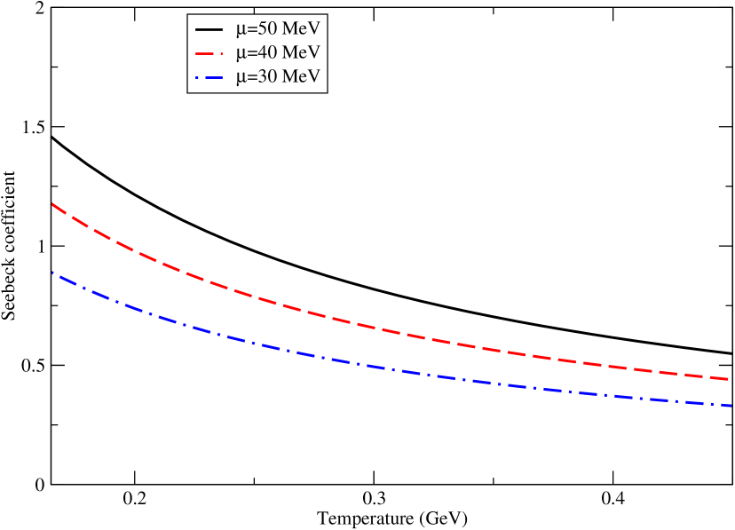
(a)

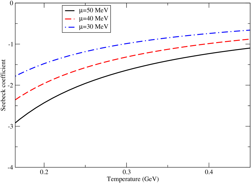
(b)

Figure 3: Variation of Seebeck coefficient of $u$ (left) and $d$ (right) quarks with temperature for different fixed values of chemical potentials.

We observe that the Seebeck coefficients (magnitudes) for $u$ and $d$ quark (Figs. 3(a) and 3(b)) decrease with the temperature for a fixed chemical potential, which is due to the fact that the net number density, ($n-\bar{n}$) (which is proportional to the net charge) decreases with the temperature for a fixed $\mu$. However, the coefficient is found to increase with chemical potential at a given temperature. This is because a larger $\mu$ is indicative of a larger surplus of particles over anti-particles, which, in the case of $u$ quark implies a larger abundance of positive over negative charges, leading to a larger thermoelectric current and hence a larger $S$. However, for the $d$ quark, a larger $\mu_{q}$ would mean a larger abundance of negative charges (particles) over positive charges (anti-particles), leading to a more negative value of $S$. Here, the sign of the Seebeck coefficient is solely determined by the sign of the electric charge the particle carries, because the other factors in the coefficient- the integrals $I_{1}$ and $I_{2}$ (eq.(57)), for both the quarks, are positive as can be seen from Fig(5) and Fig(6). The current quark masses of $u$ and $d$ quarks being very close to each other leads to almost identical values of the $I_{1}$ and $I_{2}$ integrals for both the quarks. As such, the magnitude of the electric charge of $u$ quark being twice that of $d$ quark is directly reflected in the magnitude of Seebeck coefficient of $d$ quark being almost twice that of the $u$ quark.

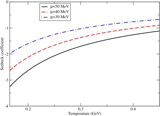
Figure 4: Variation of $s$ quark Seebeck coefficient with temperature for different fixed values of chemical potentials.

The Seebeck coefficient for $S$ quark shows the same characteristics as that of $u$ and $d$ quarks. The $I_{1}$ and $I_{2}$ integrals are positive for the $s$ quark as well. However, its mass is almost $100$ times more than that of $u$ or $d$. This leads to a larger range of $I_{1}$ and $I_{2}$ values for the $s$ quark as compared to the $d$ quark. However, the ratio $I_{1}/I_{2}$ yields values that are not too different from that of $d$ quark (Fig (5) & Fig (6)). The electric charge for the $s$ quark is the same as $d$ quark, so they exhibit close agreement in the values of respective individual Seebeck coefficients.

(a)

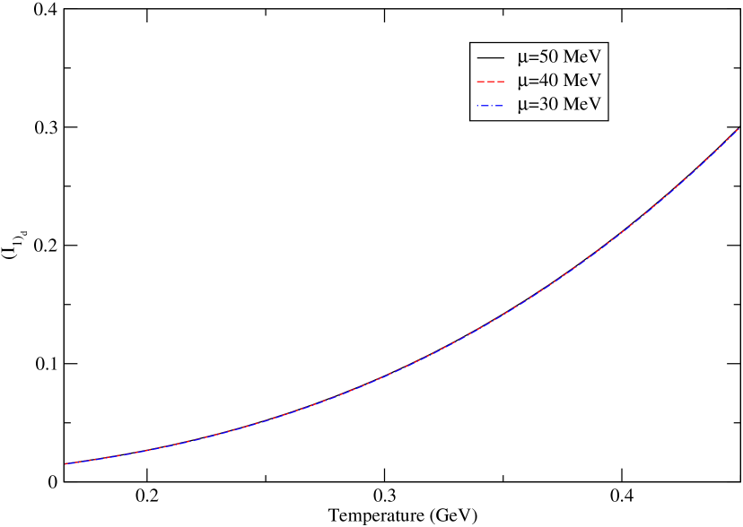
(b)

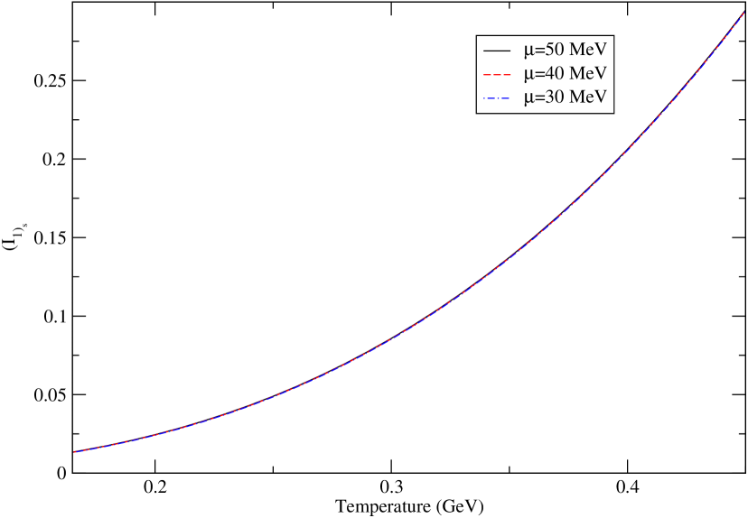
(c)

Figure 5: Variation of $I_{1}$ integrals for $u$ (left), $d$ (middle) and $s$ (right) quarks with temperature for different fixed values of chemical potential.

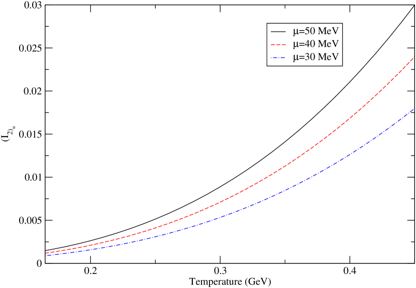
(a)

(b)

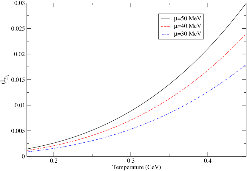
(c)

Figure 6: Variation of $I_{2}$ integrals for $u$ (left), $d$ (middle) and $s$ (right) quarks with temperature for different fixed values of chemical potential.

After having calculated the Seebeck coefficient for a thermal medium consisting of a single species, we move on to the more realistic case of a multi-component system, which in our case corresponds to multiple flavours of quarks in the QGP. However, gluons being electrically neutral, do not contribute to the thermoelectric current, therefore, the total electric current in the medium is the vector sum of currents due to individual species:

$$\vec{J} =\vec{J_{(1)}}+\vec{J_{(2)}}+\vec{J_{(3)}}+\cdots$$

$$=\left(\frac{q_{1}^{2}g_{1}\tau_{1}}{T\pi^{2}}(I_{1})_{1}+\frac{q_{2}^{2}g_{2}\tau_{1}}{T\pi^{2}}(I_{1})_{2}+...\right)\vec{E}-\bigg{(}\frac{q_{1}g_{1}\tau_{1}}{2T^{2}\pi^{2}}(I_{2})_{1}+\frac{q_{2}g_{2}\tau_{2}}{2T^{2}\pi^{2}}(I_{2})_{2}+...\bigg{)}\nabla_{\vec{r}}T(\vec{r}).$$ (58)

Setting the total current, $\vec{J}=0$ as earlier, we get the induced electric field,

$$\vec{E}=\frac{\sum_{i}\frac{q_{i}g_{i}\tau_{i}(I_{2})_{i}}{2T}}{\sum_{i}q_{i}^{2}g_{i}\tau_{i}(I_{1})_{i}}\nabla_{\vec{r}}T(\vec{r}),$$ (59)

which yields the Seebeck coefficient for the multi-component medium:

$$S=\frac{1}{2T}\frac{\sum_{i}q_{i}g_{i}\tau_{i}(I_{2})_{i}}{\sum_{i}q_{i}^{2}g_{i}\tau_{i}(I_{1})_{i}}.$$ (60)

All quarks have the same degeneracy factor and their relaxation times (seen from eq.(47)) are also identical for each flavour. Hence, the total Seebeck coefficient for the multi-component systems can be rewritten as

$$S=\frac{\sum_{i}S_{i}\,q_{i}^{2}(I_{1})_{i}}{\sum_{i}q_{i}^{2}(I_{1})_{i}},$$ (61)

which could be viewed as a weighted average of the Seebeck coefficients of individual species ($S_{i}$) present in the medium. In our calculation, we have considered only three flavours of quarks, viz: $u$, $d$ and $s$, thus, the explicit expression comes out to be:

$$S=\frac{4S_{u}(I_{1})_{u}+S_{d}(I_{1})_{d}+S_{s}(I_{1})_{s}}{4(I_{1})_{u}+(I_{1})_{d}+(I_{1})_{s}},$$ (62)

where $S_{u}$, $S_{d}$, $S_{s}$ denote the individual Seebeck coefficients for the $u$, $d$ and $s$ quarks respectively. Likewise, the $I_{1}$ integrals for different flavours are denoted by the respective flavour indices.

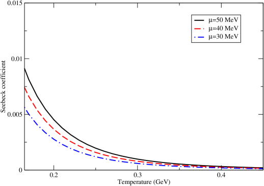
Figure 7: Variation of total Seebeck coefficient with temperature for different fixed values of chemical potentials.

As can be seen from Fig(7), the Seebeck coefficient of the medium is positive and decreases with the temperature. Like earlier for single species, it increases with the chemical potential. Although $S_{d}$ and $S_{s}$ are both negative, the relative magnitudes of $S_{u}$, $S_{d}$ and $S_{s}$ are such that eq.(62) renders the Seebeck coefficient of the medium positive with a small magnitude.

The magnitude of the Seebeck coefficient is the magnitude of electric field produced in the medium for a unit temperature-gradient. Qualitatively, it is a measure of how efficiently a medium can convert a temperature-gradient into electricity. The sign of the Seebeck coefficient expresses the direction of the induced field with respect to the direction of temperature gradient, which is conventionally taken to point towards the direction of increasing temperature. A positive value of the Seebeck coefficient means that the induced field is in the direction of the temperature-gradient. In the convention mentioned above, this will happen when the majority charge carriers are positively charged. As expected, individual Seebeck coefficient is positive for a positively charged species ($u$ quark) and negative for a negatively charged species ($d$ and $s$ quarks).

II.C Seebeck coefficient in the presence of a strong magnetic field

In the presence of magnetic field, we decompose the quark momentum into components longitudinal ($p_{L}$) and transverse ($p_{T}$) to the direction of the magnetic field. Quantum mechanically the energy levels of the $i^{\mbox{th}}$ quark flavour get discretized into Landau levels, so the dispersion relation becomes

$$\omega_{(i,n)}(p_{L})=\sqrt{p_{L}^{2}+m_{i}^{2}+2n|q_{i}B|},$$ (63)

where $n=0,1,2,\cdots$ are quantum numbers specifying the Landau levels. It is well known that in the strong magnetic field (SMF) limit (characterised by $|q_{f}B|\gg T^{2}$, where $B$ is the magnetic field and $q_{f}$ is the electric charge of the $f^{\mbox{th}}$ flavour), quarks are rarely excited thermally to higher Landau levels owing to the large energy gap between the levels, which is of the order of $\sqrt{|eB|}$[46]. Therefore, they are constrained to be populated exclusively in the lowest Landau level (n=0), implying that the quark momentum in the presence of a strong magnetic field is purely longitudinal[47, 48, 49]. Taking the magnetic field to be in the 3-direction, we identify $p_{L}$ with $p_{3}$, so the above dispersion relation is simplified into a relation for a one-dimensional free particle :

$$\omega_{i}(p_{3})=\sqrt{p_{3}^{2}+m_{i}^{2}}.$$ (64)

Thus, the equilibrium quark distribution function in SMF limit becomes:

$$f_{i,B}=\frac{1}{e^{\beta(\omega_{i}-\mu_{i})}+1}.$$ (65)

Owing to the quark momentum being purely longitudinal in the presence of a strong magnetic field, the electromagnetic current generated in response to the electric field ($J_{3}$) is also purely longitudinal.

$$J_{3}=\sum_{i}q_{i}g_{i}\int\frac{d^{3}\,\mbox{p}}{(2\pi)^{3}\,\omega_{i}}p_{3}\left[\delta f_{i}^{q}(\tilde{x},\tilde{p})-\delta f_{i}^{\bar{q}}(\tilde{x},\tilde{p})\right],$$ (66)

where, $\tilde{x}=(x_{0},0,0,x_{3})$ and $\tilde{p}=(p_{0},0,0,p_{3})$. In addition, as an artifact of strong magnetic field, the density of states in two spatial directions perpendicular to the direction of magnetic field becomes $|q_{i}B|$ [50, 51], i.e.

$$\int\frac{d^{3}p}{(2\pi)^{3}}\rightarrow\frac{q_{i}B}{2\pi}\int\frac{dp_{3}}{2\pi}.$$ (67)

The infinitesimal change in the distribution function in the strong magnetic field is thus obtained from the RBTE in the relaxation-time approximation

$$p^{0}\frac{\partial f_{i,B}}{\partial t}+p^{3}\frac{\partial f_{i,B}}{\partial x^{3}}+q_{i}F^{03}p_{3}\frac{\partial f_{i,B}}{\partial p^{0}}+q_{i}F^{30}p_{0}\frac{\partial{f_{i,B}}}{\partial{p_{3}}}=-\frac{p^{0}}{\tau^{B}}\delta f_{i,B},$$ (68)

where $\tau_{i}$ denotes the relaxation-time for quarks in the presence of strong magnetic field, which, in the Lowest Landau Level (LLL) approximation is given by[52]:

$$\tau_{i}(T,B)=\frac{w_{i}\left(e^{\beta\omega_{i}}-1\right)}{\alpha_{s}\left(\Lambda^{2},eB\right)C_{2}m_{i}^{2}\left(e^{\beta\omega_{i}}+1\right)}\left[\frac{1}{\int dp^{\prime 3}\frac{1}{w^{\prime}_{i}\left(e^{\beta\omega^{\prime}_{i}}+1\right)}}\right],$$ (69)

which has been evaluated for massless quarks. However, it has been shown in Ref.[53] that the effect of finite quark mass in the evaluation of scattering cross sections is very small, and hence, the relaxation-time is largely unaffected. $C_{2}=4/3$ is the Casimir factor. We use a one loop running coupling constant $\alpha_{s}(\Lambda^{2},eB)$, which runs with both the magnetic field and temperature. In the strong magnetic field (SMF) regime, its form is given by:[54]

$$\alpha_{s}(\Lambda^{2},|eB|)=\frac{\alpha_{s}(\Lambda^{2})}{1+b_{1}\alpha_{s}(\Lambda^{2})\,\mbox{ln}\left(\frac{\Lambda^{2}}{\Lambda^{2}+|eB|}\right)}.$$ (70)

where, $\alpha_{s}(\Lambda^{2})$ is the one- loop running coupling in the absence of a magnetic field.

$$\alpha_{s}(\Lambda^{2})=\frac{1}{b_{1}\,\mbox{ln}\left(\frac{\Lambda^{2}}{\Lambda_{QCD}^{2}}\right)},$$

where $b_{1}=(11N_{c}-2N_{f})/12\pi$ and $\Lambda_{QCD}\sim 0.2$ GeV. The renormalisation scale is chosen to be $\Lambda=2\pi\sqrt{T^{2}+\frac{\mu^{2}}{\pi^{2}T^{2}}}$. Thus, via the strong coupling, the relaxation time acquires an implicit dependence on the chemical potential.

Now, the infinitesimal change for quark and anti-quark distribution functions can be obtained from the RBTE (eq.68) in SMF regime as

$$\delta f_{i,B} =-\frac{\tau_{i}^{B}}{p^{0}}\frac{p_{z}f_{i,B}(1-f_{i,B})}{T}\left[\frac{\omega_{i}-\mu_{i}}{T}(\vec{\nabla}T)_{z}-2q_{i}E_{z}\right]$$ (71)

$$\bar{\delta f_{i,B}} =-\frac{\tau_{i}^{B}}{p^{0}}\frac{p_{z}\bar{f}_{i,B}(1-\bar{f}_{i,B})}{T}\bigg{[}\frac{\omega_{i}+\mu_{i}}{T}(\vec{\nabla}T)_{z}+2q_{i}E_{z}\bigg{]},$$ (72)

which gives the induced current density from (66) for a single species,

$$J_{z}=(\vec{\nabla}T)_{z}\left[\frac{qg|qB|}{T(2\pi)^{2}}\int\frac{dp_{z}}{\omega^{2}}p_{z}^{2}(\tau^{B})\left\{\bar{f}(1-\bar{f})\frac{\omega+\mu}{T}-f(1-f)\frac{\omega-\mu}{T}\right\}\right]\\ -2qE_{z}\left[\frac{qg|qB|}{T(2\pi)^{2}}\int\frac{dp_{z}}{\omega^{2}}p_{z}^{2}(\tau^{B})\left\{\bar{f}(1-\bar{f})+f(1-f)\right\}\right],$$ (73)

where, $g$ is the degeneracy factor. Defining the following integrals

$$H_{1} = \int\frac{dp_{z}}{w_{i}^{2}}\,\tau_{B}^{i}\,p_{z}^{2}\left\{-\bar{f}(1-\bar{f})(\omega+\mu)+f(1-f)(\omega-\mu)\right\},$$ (74)

$$H_{2} = \int\frac{dp_{z}}{w_{i}^{2}}\,\tau_{B}^{i}\ ,p_{z}^{2}\left\{\bar{f}(1-\bar{f})+f(1-f)\right\},$$ (75)

the current density (3rd-component) from eq.(73) can be recast in the form

$$J_{z}=(\vec{\nabla}T)_{z}\,\frac{qg|qB|}{T^{2}(2\pi)^{2}}H_{1}-E_{z}\,\frac{qg|qB|}{T(2\pi)^{2}}2qH_{2}$$ (76)

As earlier, the induced electric field due to the temperature-gradient is obtained by setting $J_{z}=0$,

$$E_{z}=\frac{1}{2Tq}\frac{H_{1}}{H_{2}}(\vec{\nabla}T)_{z}.$$ (77)

The proportionally constant gives the Seebeck coefficient:

$$S=\frac{1}{2Tq}\frac{H_{1}}{H_{2}}$$ (78)

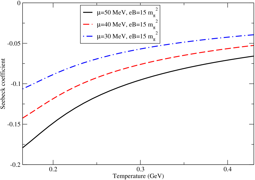
(a)

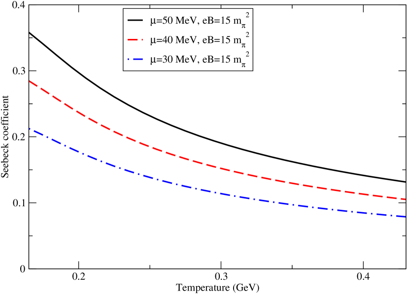
(b)

Figure 8: Variation of Seebeck coefficient of $u$ (left) and $d$ (right) quarks with temperature for a fixed chemical potential and magnetic field.

As can be seen from Fig.(8), the variation of the individual Seebeck coefficients (magnitudes) of the $u$ and $d$ quarks with temperature and chemical potential shows the same trend as in the earlier case. However, the sign of the Seebeck coefficient in this case is negative for $u$ quark and positive for $d$ quark. This is opposite to what was encountered earlier. This is because the $H_{1}$ integrals for both $u$ and $d$ quarks turn out to be negative in this case (Fig.(10)) and the $H_{2}$ integrals positive (Fig.(11)). Considered along with the dependence on the particle charge, this explains the sign of the Seebeck coefficient for $u$ and $d$ quarks. The Seebeck coefficients for the $u$ and $d$ quarks in this case turn out to be about 1 order of magnitude smaller, compared to their $B=0$ counterparts.

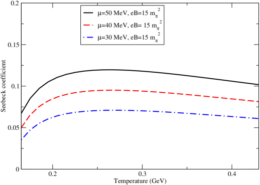
Figure 9: Variation of $s$ quark Seebeck coefficient with temperature for a fixed magnetic field and different fixed values of chemical potential.

The sign of the $s$ quark Seebeck coefficient is again opposite to that of the $B=0$ case owing to the $H_{1}$ integral for $s$ quark being negative. The magnitude of the Seebeck coefficient rises with temperature upto about $T=270$ MeV and starts decreasing therefrom. Although the ratio $H_{1}/H_{2}$ is an increasing function of $T$ for the entire temperature range, it does not increase fast enough after $T=270$ MeV to compensate for the rising temperature (in the denominator of $S$; eq.(78)).

It should be noted that contrary to the case of pure thermal medium, the relaxation time here is momentum dependent. As such, it cannot be taken out of the momentum integrations ($H_{1},H_{2}$) and hence does not cancel out in $S$.

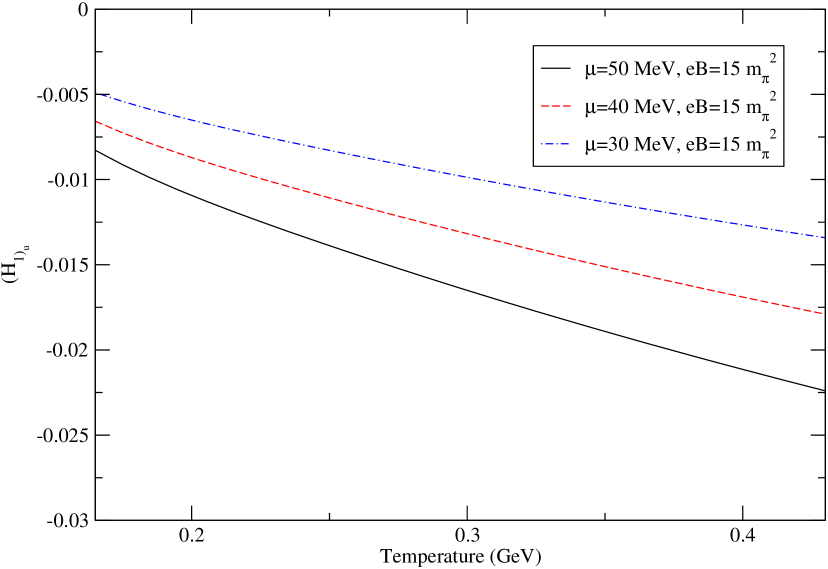
(a)

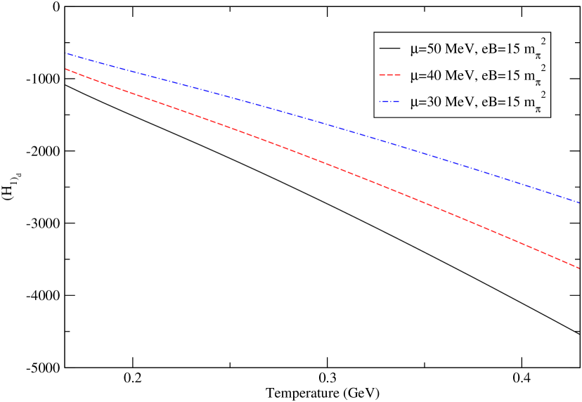
(b)

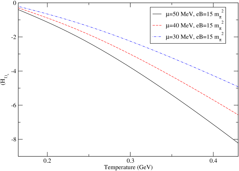
(c)

Figure 10: Variation of $H_{1}$ integrals for $u$ (left), $d$ (middle) and $s$ (right) quarks with temperature

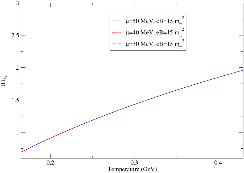
(a)

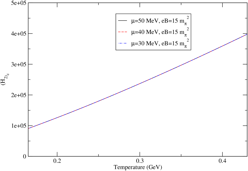
(b)

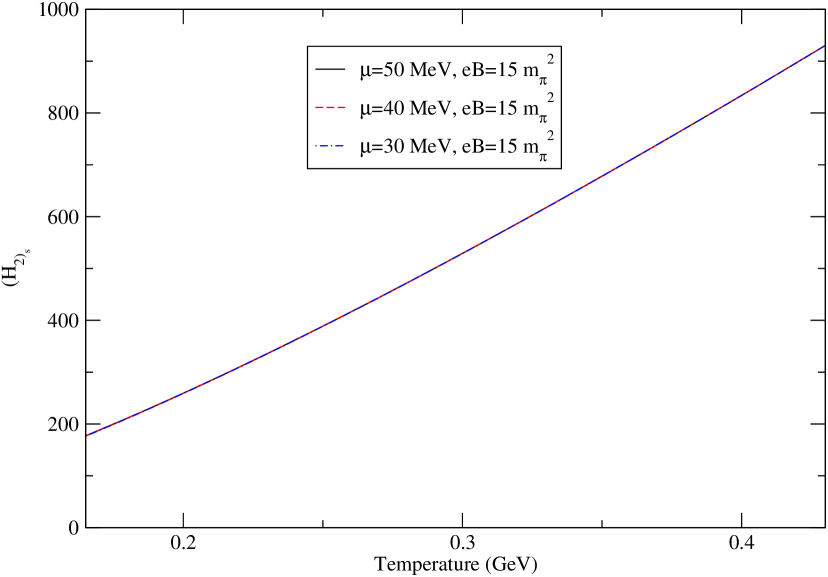
(c)

Figure 11: Variation of $H_{2}$ integrals for $u$ (left), $d$ (middle) and $s$ (right) quarks with temperature.

Now we generalize our formalism to a medium consisting of multiple species, therefore, the total current is given by the sum of currents due to individual species:

$$J_{z} = J_{z}^{1}+J_{z}^{2}+J_{z}^{3}+\cdots$$ (79)

$$= (\vec{\nabla}T)_{z}\left\{\frac{q_{1}g_{1}|q_{1}B|}{T^{2}(2\pi)^{2}}(H_{1})_{1}+\frac{q_{2}g_{2}|q_{2}B|}{T^{2}(2\pi)^{2}}(H_{1})_{2}+\frac{q_{3}g_{3}|q_{3}B|}{T^{2}(2\pi)^{2}}(H_{1})_{3}+\cdots\right\}$$

$$- E_{z}\left\{\frac{q_{1}g_{1}|q_{1}B|}{T(2\pi)^{2}}2q_{1}(H_{2})_{1}+\frac{q_{2}g_{2}|q_{2}B|}{T(2\pi)^{2}}2q_{2}(H_{2})_{2}+\frac{q_{3}g_{3}|q_{3}B|}{T(2\pi)^{2}}2q_{3}(H_{2})_{3}+\cdots\right\}$$

Again, the Seebeck coefficient of the medium in a strong magnetic field is obtained by setting $J_{z}=0$,

$$S=\frac{1}{2T}\frac{\sum_{i}q_{i}|q_{i}B|(H_{1})_{i}}{\sum_{i}q_{i}^{2}|q_{i}B|(H_{2})_{i}},$$ (80)

which could be further expressed in terms of the weighted average of individual Seebeck coefficients.

$$S=\frac{\sum_{i}S_{i}|q_{i}|^{3}(H_{2})_{i}}{\sum_{i}|q_{i}|^{3}(H_{2})_{i}}.$$ (81)

Thus, unlike the Seebeck coefficient in the absence of magnetic field (eq.57), both the individual as well as total Seebeck coefficient of the medium depend on the relaxation-time in the presence of a strong magnetic field.

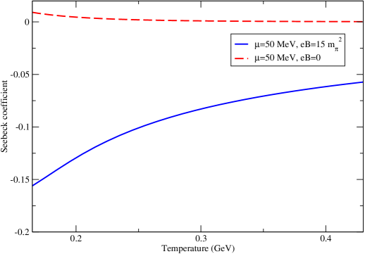
Figure 12: Variation of Seebeck coefficient of the medium with temperature for a fixed chemical potential in the absence and presence of a magnetic field.

We can now visualize the sole effect of strong magnetic field on the (total) Seebeck coefficient from the comparison of $B\neq 0$ and $B=0$ results in Fig.(12). Unlike the $B=0$ (red line) case, the total Seebeck coefficient in strong $B$ (black line) becomes negative, indicating that the induced electric field is opposite to the direction of temperature-gradient. However, the magnitude of total Seebeck coefficient decreases with the temperature and increases with the chemical potential, much like, the $B=0$ case. However, the strong magnetic field enhances the magnitude of $S$ by one order of magnitude, compared to the $B=0$ case.

III Seebeck effect of hot partonic medium in a quasiparticle model

Quasiparticle description of quarks and gluons in a thermal QCD medium in general, introduces a thermal mass, apart from their current masses in QCD Lagrangian. These masses are generated due to the interaction of a given parton with other partons in the medium, therefore, quasiparticle description in turn describes the collective properties of the medium. However, in the presence of strong magnetic field in the thermal QCD medium, different flavors acquire masses differently due to their different electric charges. Different versions of quasiparticle description exist in the literature based on different effective theories, such as Nambu-Jona-Lasinio (NJL) model and its extension PNJL model [55, 56, 57], Gribov-Zwanziger quantization [58, 59], thermodynamically consistent quasiparticle model [60], etc. However, our description relies on perturbative thermal QCD, where the medium generated masses for quarks and gluons are obtained from the poles of dressed propagators calculated by the respective self-energies at finite temperature and/or strong magnetic field.

III.A Seebeck coefficient in the absence of magnetic field

In the quasiparticle description of quarks and gluons in a thermal medium with $3$ flavours, all flavours (with current/vacuum masses, $m_{i}<<T$) acquire the same thermal mass [61, 62]

$$m_{T}^{2}=\frac{g^{2}(T)T^{2}}{6},$$ (82)

which is, however, modified in the presence of a finite chemical potential [63]

$$m_{T,\mu}^{2}=\frac{g^{2}(T)T^{2}}{6}\left(1+\frac{\mu^{2}}{\pi^{2}T^{2}}\right),$$ (83)

where $g$ is the running coupling constant already mentioned in eq.(48).

We take the quasiparticle mass (squared) of $i^{\mbox{th}}$ flavor in a pure thermal medium to be [60]:

$$m_{iT}^{\prime~{}2}=m_{i}^{2}+\sqrt{2}\,m_{i}\,m_{T}+m_{T}^{2},$$ (84)

where $m_{i}$ is the current quark mass of the $i^{\mbox{th}}$ flavour. So the dispersion relation for the $i^{\mbox{th}}$ flavour takes the form

$$\omega_{i}^{2}(p)=\vec{p_{i}}^{\,\,2}+m_{i}^{2}+\sqrt{2}\,m_{i}\,m_{T}+m_{T}^{2}.$$ (85)

Using this expression of $\omega_{i}(p)$ in the quark distribution functions as well as in the integrals $I_{1}$ and $I_{2}$ (eq.56), we proceed in a similar fashion and evaluate the individual Seebeck coefficients for the $u$, $d$ and $s$ quarks in quasiparticle description from eq.(57)

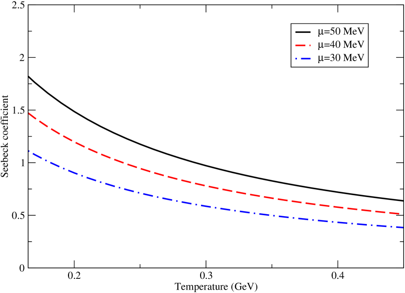
(a)

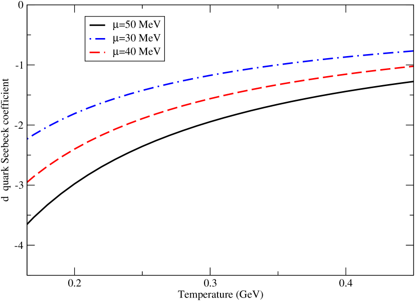
(b)

Figure 13: Variation of Seebeck coefficient of $u$ (left) and $d$ (right) quarks with temperature for different fixed values of chemical potentials.

As can be seen from Figs. 13(a) and 13(b), the Seebeck coefficients of $u$ and $d$ quarks show a trend similar to their current quark mass counterparts in the absence of magnetic field (Figs. 3(a) & 3(b)) and their magnitudes decrease with temperature and increase with chemical potential. The $I_{1}$ and $I_{2}$ integrals for both quarks are also found to be positive and as such, the sign of the coefficient is again determined by the electric charge of the particle. The change due to the quasiparticle description adopted here, is a slight increase in the magnitudes of the Seebeck coefficients for both quarks.

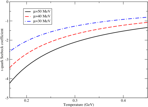
Figure 14: Variation of $s$ quark Seebeck coefficient with temperature for different fixed values of chemical potentials.

Similar to the current quark mass case (in Fig. 4), the coefficient for $s$ quark decreases in magnitude with increasing temperature (Fig. 14). Owing to its negative electric charge and the positive value of $I_{1}$, $I_{2}$ integrals, the sign of the coefficient is negative. Thus, the overall behaviour of individual Seebeck coefficients in the quasiparticle description is similar to that of the current mass description with slightly enhanced magnitudes. Numerically the average percentage increase for the $u$, $d$ and $s$ quarks are around 19.52%, 19.70% and 24.38%, respectively.

Similarly, the total Seebeck coefficient of the medium in quasiparticle description

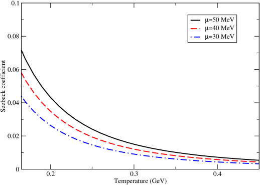
Figure 15: Variation of Seebeck coefficient of the medium with temperature for different fixed values of chemical potential.

(in Fig. 15) is found to have a small positive value, which decreases with the temperature and increases with the chemical potential as earlier, but with a significantly elevated magnitude in comparison with the current quark mass case (in Fig 7).

III.B Seebeck coefficient in the presence of strong magnetic field

In the presence of magnetic field, only quarks are affected while the gluons are not directly influenced. As a result, only the quark-loop of the gluon self-energy will be affected and the gluon-loops remains altered. Furthermore, only quarks contribute to the thermoelectric effect, and hence, we proceed to calculate the thermal quark mass in the presence of a strong magnetic field, which can be obtained from the pole ($p_{0}=0,\mathbf{p}\rightarrow 0$ limit) of the full propagator.

As we know, the full quark propagator can be obtained self-consistently from the Schwinger-Dyson equation (assuming massless flavours, which is assumed to be true at least for light flavours),

$$S^{-1}(p_{\parallel})=\gamma^{\mu}p_{\parallel\mu}-\Sigma(p_{\parallel})~{},$$ (86)

where $\Sigma(p_{\parallel})$ is the quark self-energy at finite temperature in the presence of strong magnetic field. We can evaluate it up to one-loop

$$\Sigma(p)=-\frac{4}{3}g_{s}^{2}i\int{\frac{d^{4}k}{(2\pi)^{4}}}\left[\gamma_{\mu}{S(k)}\gamma_{\nu}{D^{\mu\nu}(p-k)}\right],$$ (87)

where $4/3$ denotes the Casimir factor and $g_{s}=\sqrt{4\pi\alpha_{s}}$ represents the running coupling with the $\alpha_{s}$ already defined in Eq.(70). $D^{\mu\nu}(p-k)$ is the gluon propagator, which is not affected by the magnetic field, so its form is given by

$$D^{\mu\nu}(p-k)=\frac{ig^{\mu\nu}}{{(p-k)}^{2}}~{}.$$ (88)

However, the quark propagator, $S(K)$ in the strong magnetic field limit, is affected and is obtained by the Schwinger proper-time method at the lowest Landau level (n=0) in momentum space,

$$S(k)=ie^{-\frac{k^{2}_{\perp}}{|q_{i}B|}}\frac{\left(\gamma^{0}k_{0}-\gamma^{3}k_{z}+m_{i}\right)}{k^{2}_{\parallel}-m^{2}_{i}}\left(1-\gamma^{0}\gamma^{3}\gamma^{5}\right),$$ (89)

where the 4-vectors are defined as $k_{\perp}\equiv(0,k_{x},k_{y},0),~{}~{}k_{\parallel}\equiv(k_{0},0,0,k_{z})$.

Next we obtain the form of quark and gluon propagators at finite temperature in the imaginary-time formalism and subsequently replace the energy integral ($\int\frac{dp_{0}}{2\pi}$) by Matsubara frequency sum. However, in a strong magnetic field along $z$-direction, the transverse component of the momentum becomes vanishingly small ($k_{\perp}\approx 0$), so the exponential factor in eq.(89) becomes unity and the integration over the transverse component of the momentum becomes $|q_{f}B|$. Thus, the quark self-energy in eq.(87) at finite temperature in the SMF limit will be of the form

$$\Sigma(p_{\parallel}) = \frac{2g_{s}^{2}}{3\pi^{2}}|q_{i}B|T\sum_{n}\int dk_{z}\frac{\left[\left(1+\gamma^{0}\gamma^{3}\gamma^{5}\right)\left(\gamma^{0}k_{0}-\gamma^{3}k_{z}\right)-2m_{i}\right]}{\left[k_{0}^{2}-\omega^{2}_{k}\right]\left[(p_{0}-k_{0})^{2}-\omega_{pk}^{2}\right]}$$ (90)

$$= \frac{2g_{s}^{2}|q_{i}B|}{3\pi^{2}}\int dk_{z}\left[(\gamma^{0}+\gamma^{3}\gamma^{5})L^{1}-(\gamma^{3}+\gamma^{0}\gamma^{5})k_{z}L^{2}\right],$$

where $\omega^{2}_{k}=k_{z}^{2}+m_{i}^{2}$,  $\omega_{pk}^{2}=(p_{z}-k_{z})^{2}$ and $L^{1}$ and $L^{2}$ are the two frequency sums, which are given by

$$L^{1}=T\sum_{n}k_{0}~{}\frac{1}{\left[k_{0}^{2}-\omega_{k}^{2}\right]}\frac{1}{\left[(p_{0}-k_{0})^{2}-\omega_{pk}^{2}\right]}~{},$$ (91)

$$L^{2}=T\sum_{n}\frac{1}{\left[k_{0}^{2}-\omega_{k}^{2}\right]}\frac{1}{\left[(p_{0}-k_{0})^{2}-\omega_{pk}^{2}\right]}~{}.$$ (92)

We first do the frequency sums [64, 41] and then integrate the momentum $k_{z}$ to obtain the simplified form of quark self-energy eq.(90) [65] as

$$\Sigma(p_{\parallel})=\frac{g_{s}^{2}|q_{i}B|}{3\pi^{2}}\left[\frac{\pi T}{2m_{i}}-\ln(2)\right]\left[\frac{\gamma^{0}p_{0}}{p_{\parallel}^{2}}+\frac{\gamma^{3}p_{z}}{p_{\parallel}^{2}}+\frac{\gamma^{0}\gamma^{5}p_{z}}{p_{\parallel}^{2}}+\frac{\gamma^{3}\gamma^{5}p_{0}}{p_{\parallel}^{2}}\right].$$ (93)

To solve the Schwinger-Dyson equation eq.(86), one needs to first express the self-energy at finite temperature in magnetic field in a covariant form [66, 67],

$$\Sigma(p_{\parallel})=A{(\rm p_{0},\bf p)}\gamma^{\mu}u_{\mu}+B{(\rm p_{0},\bf p)}\gamma^{\mu}b_{\mu}+C{(\rm p_{0},\bf p)}\gamma^{5}\gamma^{\mu}u_{\mu}+D{(\rm p_{0},\bf p)}\gamma^{5}\gamma^{\mu}b_{\mu}~{},$$ (94)

where $u^{\mu}$ (1,0,0,0) and $b^{\mu}$ (0,0,0,-1) denote the preferred directions of heat bath and magnetic field, respectively and these vectors mimic the breaking of Lorentz and rotational invariances, respectively. The form factors, $A$, $B$, $C$ and $D$ are computed in strong $B$ with LLL approximation as

$$A=\frac{g_{s}^{2}|q_{i}B|}{3\pi^{2}}\left[\frac{\pi T}{2m_{i}}-\ln(2)\right]\frac{p_{0}}{p_{\parallel}^{2}}~{},$$ (95)

$$B=\frac{g_{s}^{2}|q_{i}B|}{3\pi^{2}}\left[\frac{\pi T}{2m_{i}}-\ln(2)\right]\frac{p_{z}}{p_{\parallel}^{2}}~{},$$ (96)

$$C=-\frac{g_{s}^{2}|q_{i}B|}{3\pi^{2}}\left[\frac{\pi T}{2m_{i}}-\ln(2)\right]\frac{p_{z}}{p_{\parallel}^{2}}~{},$$ (97)

$$D=-\frac{g_{s}^{2}|q_{i}B|}{3\pi^{2}}\left[\frac{\pi T}{2m_{i}}-\ln(2)\right]\frac{p_{0}}{p_{\parallel}^{2}}~{}.$$ (98)

Then the self-energy (94) can be expressed in terms of chiral projection operators ($P_{R}$ and $P_{L}$) as

$$\Sigma(p_{\parallel})=P_{R}\left[(A-B)\gamma^{\mu}u_{\mu}+(B-A)\gamma^{\mu}b_{\mu}\right]P_{L}+P_{L}\left[(A+B)\gamma^{\mu}u_{\mu}+(B+A)\gamma^{\mu}b_{\mu}\right]P_{R}~{}.$$ (99)

Hence, the Schwinger-Dyson equation is able to express the inverse of the full propagator in terms of $P_{L}$ and $P_{R}$,

$$S^{-1}(p_{\parallel})=P_{R}\gamma^{\mu}X_{\mu}P_{L}+P_{L}\gamma^{\mu}Y_{\mu}P_{R}~{},$$ (100)

where

$$\gamma^{\mu}X_{\mu}=\gamma^{\mu}p_{\parallel\mu}-(A-B)\gamma^{\mu}u_{\mu}-(B-A)\gamma^{\mu}b_{\mu}~{},$$ (101)

$$\gamma^{\mu}Y_{\mu}=\gamma^{\mu}p_{\parallel\mu}-(A+B)\gamma^{\mu}u_{\mu}-(B+A)\gamma^{\mu}b_{\mu}~{}.$$ (102)

Thus, the effective propagator is finally obtained by inverting eq. (100)

$$S(p_{\parallel})=\frac{1}{2}\left[P_{R}\frac{\gamma^{\mu}Y_{\mu}}{Y^{2}/2}P_{L}+P_{L}\frac{\gamma^{\mu}X_{\mu}}{X^{2}/2}P_{R}\right],$$ (103)

where

$$\frac{X^{2}}{2}=X_{1}^{2}=\frac{1}{2}\left[p_{0}-(A-B)\right]^{2}-\frac{1}{2}\left[p_{z}+(B-A)\right]^{2}~{},$$ (104)

$$\frac{Y^{2}}{2}=Y_{1}^{2}=\frac{1}{2}\left[p_{0}-(A+B)\right]^{2}-\frac{1}{2}\left[p_{z}+(B+A)\right]^{2}~{}.$$ (105)

Thus, the thermal mass (squared) for $i^{\mbox{th}}$ flavor at finite temperature and strong magnetic field is finally obtained by taking the $p_{0}=0,p_{z}\rightarrow 0$ limit in either $X_{1}^{2}$ or $Y_{1}^{2}$ (because both of them are equal),

$$m_{iT,B}^{2}=\frac{g_{s}^{2}|q_{i}B|}{3\pi^{2}}\left[\frac{\pi T}{2m_{i}}-\ln(2)\right],$$ (106)

which depends both on temperature and magnetic field. The quark distribution functions with medium generated masses in the absence and presence of magnetic field therefore manifest the interactions present in the respective medium in terms of modified occupation probabilities in the phase space and thus affect the Seebeck coefficients. The quasiparticle (or effective) mass of $i^{\mbox{th}}$ quark flavor is generalized in finite temperature and strong magnetic field into

$$m_{i~{}T,B}^{\prime~{}2}=m_{i}^{2}+\sqrt{2}\,m_{i}\,m_{iT,B}+m_{iT,B}^{2}.$$ (107)

Now, using the above quasiparticle mass in the distribution function and proceeding identically, we compute the individual Seebeck coefficients from eq.(78) as a function of temperature, which is shown in Fig. 16.

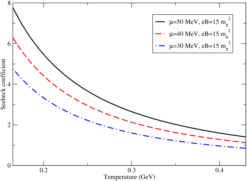
(a)

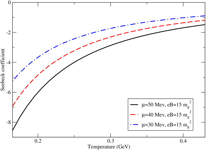
(b)

Figure 16: Variation of Seebeck coefficient of $u$ (left) and $d$ (right) quarks with temperature for a fixed chemical potential and magnetic field.

We find that the magnitudes of both $u$ and $d$ quark Seebeck coefficients decrease with the temperature and increase with the chemical potential. In quasiparticle description, the $H_{1}$ integrals for both $u$ and $d$ quarks becomes positive, unlike the case with current quark masses in strong $B$ (Fig. 8), so the sign of the individual Seebeck coefficient is decided only by the electric charge of quarks, similar to the $B=0$ case. The magnitudes of the Seebeck coefficients are found to increase by two-order of magnitude over their current quark mass case counterparts (seen in Fig. 8), which could thus be attributed to the quasiparticle description.

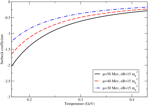
Figure 17: Variation of $s$ quark Seebeck coefficient with temperature for a fixed magnetic field and different fixed values of chemical potential.

The sign of the Seebeck coefficient for $s$-quark in quasiparticle description now becomes negative, opposite to the case of current quark mass description (Fig.9 ). Again, this is because the quasiparticle description flips the signs of $H_{1}$ integral for the $s$ quark from negative (in Fig.10) to positive, so the deciding factor for the sign of the coefficient is the sign of the electric charge of $s$ quark (which is negative). Furthermore, the variation of the magnitude of Seebeck coefficient with temperature in quasiparticle description is quite different compared to the current quarks mass case (Fig.9) and is rather similar to that of $d$ quark (Fig. 16(b)) but with smaller magnitude.

Comparison between the $B=0$ and $B\neq 0$ results within the quasiparticle description reveals summarily that the percentage increase is more pronounced at lower temperatures. The average percentage increase over the entire temperature range is 467.61% and 212.63% for $u$ and $d$ quarks, respectively. However, the percentage increase for $s$ quark is -36.81%, suggesting that the $s$ quark Seebeck coefficient in the presence of a strong $B$ is smaller in magnitude than its pure thermal ($B=0$) counterpart (Fig.14). Hence, in the presence of strong $B$, the Seebeck effect depends strongly on the interactions among the constituents in the medium, encoded by the appropriate quasiparticle description.

(a)

(b)

(c)

Figure 18: Variation of $H_{1}$ integrals for $u$ (left), $d$ (middle) and $s$ (right) quarks with temperature for different fixed values of chemical potential.

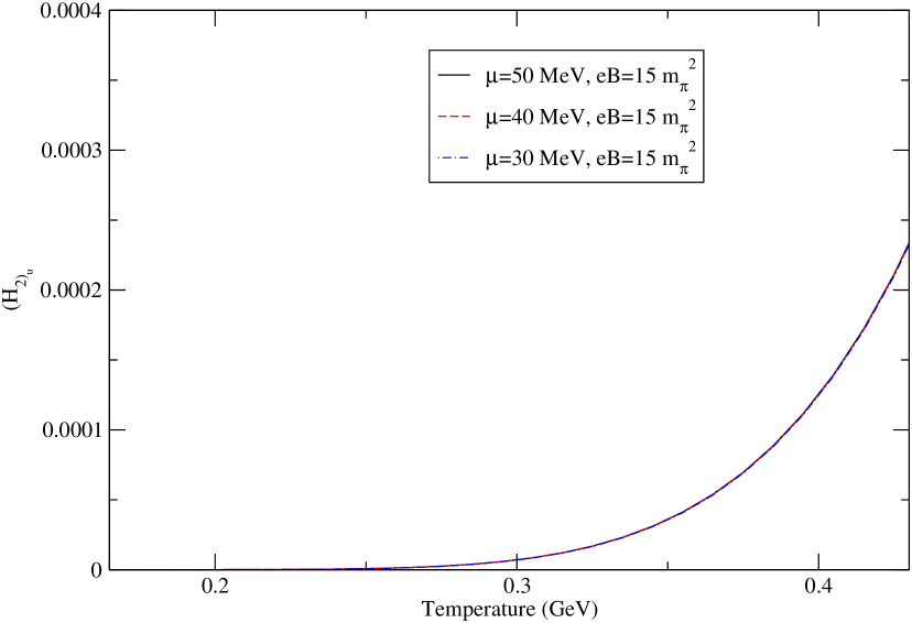
(a)

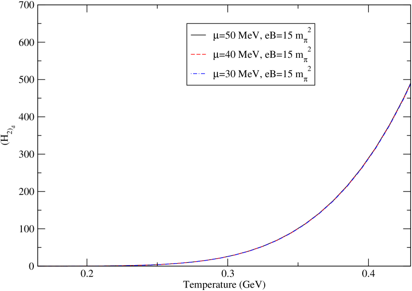
(b)

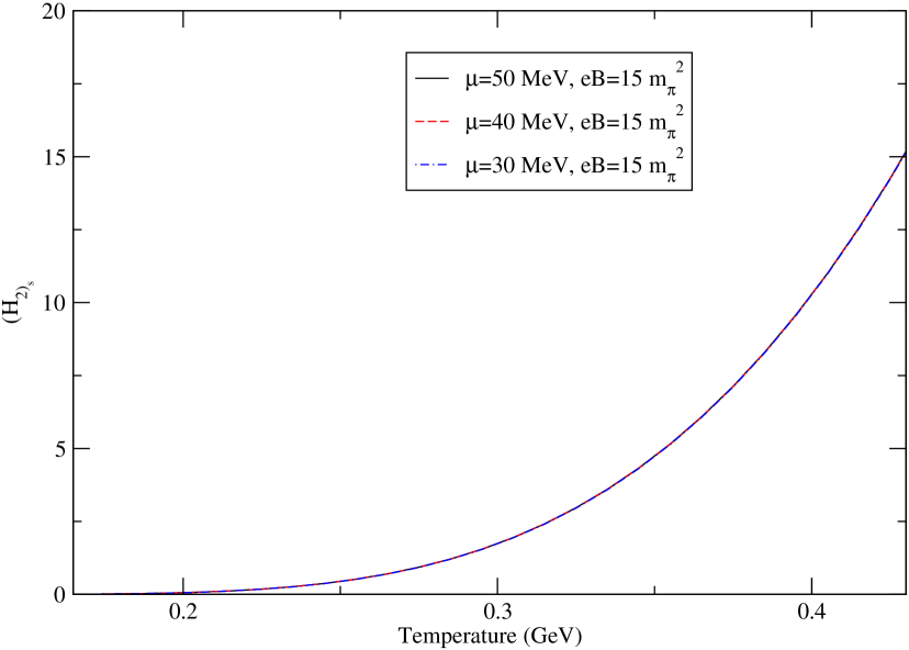
(c)

Figure 19: Variation of $H_{2}$ integrals for $u$ (left), $d$ (middle) and $s$ (right) quarks with temperature for different fixed values of chemical potential.

Once the individual Seebeck coefficients of $u$, $d$ and $s$ quarks have been evaluated in quasiparticle description, we compute the weighted average of the above individual coefficients to obtain the (total) Seebeck coefficient of the medium as a function of temperature from eq.(81). This is shown in Fig. 20. To see the effects of magnetic field in quasiparticle description, we have also displayed the same in the absence of magnetic field (shown by black solid line in Fig. 15) in the same figure for better visual effects.

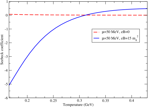
Figure 20: Variation of Seebeck coefficient of the medium with temperature for a fixed chemical potential in the absence and presence of a magnetic field.

The seebeck coefficient starts out negative and one order of magnitude larger than its immediate counterpart in the absence of magnetic field. The magnitude decreases rapidly with increasing temperature, eventually crosses the zero mark and continues to higher positive values thereafter. Physically, the direction of the induced field is opposite to that of the temperature gradient to start with. As the temperature rises, the strength of this field gets weaker. At a particular value of the temperature, the individual seebeck coefficients have values so as to make the weighted average zero. For still higher values of temperature, the weighted average becomes positive, indicating that the induced electric field is now along the temperature gradient.

IV Summary and conclusions

In this paper, we have investigated the thermoelectric phenomenon of Seebeck effect in a hot QCD medium in two descriptions: i) when the quarks are treated in QCD with their current masses and ii) when the quarks are treated in quasiparticle model. The emergence of a strong magnetic field in the non-central events of the ultra-relativistic heavy ion collisions provides a further impetus to carry out the aforesaid investigations both in the absence and presence of a strong magnetic field, in order to isolate the effects of strong magnetic fields and interactions present among partons. For this purpose, the Seebeck coefficients are calculated individually for the $u$, $d$ and $s$ quarks, which, in turn, give the Seebeck coefficient of the medium via a weighted average of the individual coefficients. Thus, effectively, four different scenarios have been analysed:

1. Current mass description with $B=0$.

2. Current mass description with $B\neq 0$.

3. Quasiparticle description with $B=0$.

4. Quasiparticle description with $B\neq 0$.

Comparison between the cases 1 and 3 is able to decipher the effect of the intereactions among the partons through the quasiparticle description on the Seebeck effect in the absence of strong magnetic field, where the magnitudes of Seebeck coefficient of individual species as well as that of the medium get(s) sightly enhanced with respect to the current mass description. The sign of the individual Seebeck coefficients is positive for positively charged particles ($u$ quark) and negative for negatively charged particles ($d$ and $s$ quarks) except for the case 2, where, owing to the $H_{1}$ integral becoming negative (for each quark), the situation is reversed. Comparison between cases 2 and 4 brings out the sole effect of the quasiparticle description in the presence of a strong magnetic field, where it is seen that the magnitude of the coefficients are amplified. The sign of the Seebeck coefficient of the medium, is however same in both the cases. Lastly, the comparison between cases 3 and 4 brings forth the sole effect of strong constant magnetic field on the Seebeck effect in the quasiparticle description. The variation of individual and total Seebeck coefficients with temperature and chemical potential are found to show similar trends in both the cases but with enhanced magnitudes in the latter case.

The trend of overall decrease (increase) of the magnitude of Seebeck coefficient with the increase in temperature (chemical potential) is seen for all cases. However, in the quasiparticle description, the magnitude of the coefficient gets enhanced in the presence of strong magnetic field, so the inclusion of interactions among partons plays a crucial role in thermoelectric phenomenon in thermal QCD.

V Acknowledgements

We are thankful to Sumit and Pushpa for their fruitful discussin in the calculaton for the matrix element. BKP is thankful to the Council of Scientific and Industrial Research Grant No.03 (1407)/17/EMR-II), Government of India for the financial assistance.

Appendix A Matrix Element for gluon-gluon scattering in vacuum

We will study the scattering in Figs. 1 and 2 in the cm frame with the four momenta for incoming particles as $K_{1}(k_{1}^{0},\vec{k_{1}})$ and $K_{2}(k_{2}^{0},\vec{k}_{2})$, and that for outgoing particles as $K_{3}(k_{3}^{0},\vec{k_{3}})$ and $K_{4}(k_{4}^{0},\vec{k_{4}})$. Moreover, we assume that the trajectory of the incoming particles is along the $z$-direction and the scattered particles lie in the $x$-$z$ plane, such that $\hat{k_{3}}.\hat{z}=\mbox{cos}\,\theta$ (where, $\hat{k_{3}}=\frac{\vec{k_{3}}}{k_{3}}$). The external gluons are lightlike, viz. $K_{i}^{2}=0$, i.e. $k_{i}=(k_{i})_{z}=\epsilon$, where $\epsilon$ is the energy of the gluons and $i=1,2,3,4.$ Thus the four momenta of the external gluons are written as:

$$K_{1}(k_{1}^{0},\vec{k_{1}}) \equiv K_{1}(\epsilon,0,0,\epsilon)\,,\qquad\qquad\qquad\qquad K_{2}(k_{2}^{0},\vec{k}_{2})\equiv K_{2}(\epsilon,0,0,-\epsilon)\,$$

$$K_{3}(k_{3}^{0},\vec{k_{3}}) \equiv K_{3}(\epsilon,\epsilon\,\mbox{sin}\,\theta,0,\epsilon\,\mbox{cos}\,\theta)\,,\qquad\quad K_{4}(k_{4}^{0},\vec{k_{4}})\equiv K_{4}(\epsilon,-\epsilon\,\mbox{sin}\,\theta,0,-\epsilon\,\mbox{cos}\,\theta).$$ (108)

Since the polarisations of the external gluons are transverse to the respective four-momenta, so we could write the polarisation vectors as

$$\epsilon^{\mu}_{\lambda_{1}}(K_{1}) =\frac{1}{\sqrt{2}}(0,1,\pm i,0)\,,\qquad\qquad\qquad\quad\epsilon^{\mu}_{\lambda_{2}}(K_{2})=\frac{1}{\sqrt{2}}(0,-1,\pm i,0)\,$$

$$\epsilon^{\mu\,*}_{\lambda_{3}}(K_{3}) =\frac{1}{\sqrt{2}}(0,-\mbox{cos}\,\theta,\pm i,\mbox{sin}\,\theta)\,,\qquad\quad\,\epsilon^{\mu\,*}_{\lambda_{4}}(K_{4})=\frac{1}{\sqrt{2}}(0,\mbox{cos}\,\theta,\pm i,-\mbox{sin}\,\theta),$$ (109)

where, $\lambda_{1}$, $\lambda_{2}$ are the polarizations of incoming gluons and $\lambda_{3}$ and $\lambda_{4}$ are the same for the outgoing (scattered) gluons. Since the gluons in vacuum are massless, the $\lambda_{i}$’s can only be either right-handed (R) or left-handed polarizations (L).

We begin with the $s$ channel diagram in Fig.1(a). Using the Feynman rules, we write the matrix element for it as

$$i\mathcal{M}_{s}=-ig_{s}^{2}f^{abc}f^{cde}\epsilon_{\mu}^{\lambda_{1}}(K_{1})\epsilon_{\nu}^{\lambda_{2}}(K_{2})\epsilon_{\rho}^{*\lambda_{3}}(K_{3})\epsilon_{\sigma}^{*\lambda_{4}}(K_{4})\Big{[}g^{\mu\nu}(K_{1}-K_{2})^{\alpha}+g^{\nu\alpha}(K_{1}+2K_{2})^{\mu}$$

$$+g^{\alpha\mu}(-2K_{1}-K_{2})^{\nu}\Big{]}\times\left(\frac{-ig_{\alpha\alpha^{\prime}}}{{(K_{1}+K_{2})}^{2}}\right)\left[g^{\rho\sigma}(-K_{3}+K_{4})^{\alpha^{\prime}}+g^{\sigma\alpha^{\prime}}(-K_{3}-2K_{4})^{\rho}+g^{\alpha^{\prime}\rho}(2K_{3}+K_{4})^{\sigma}\right],$$ (110)

which takes the form, after contracting the lorentz indices,

$$i\mathcal{M}_{s} =\frac{-ig_{s}^{2}f^{abc}f^{cde}}{(K_{1}+K_{2})^{2}}\Big{[}\epsilon^{\lambda_{1}}(K_{1})\cdot\epsilon^{\lambda_{2}}(K_{2})\times(K_{2}-K_{1})\cdot(K_{3}-K_{4})\times\epsilon^{*\lambda_{3}}(K_{3})\cdot\epsilon^{*\lambda_{4}}(K_{4})$$

$$+\epsilon^{\lambda_{1}}(K_{1})\cdot(K_{1}+2K_{2})\times\epsilon^{\lambda_{2}}(K_{2})\cdot(K_{4}-K_{3})\times\epsilon^{*\lambda_{3}}(K_{3})\cdot\epsilon^{*\lambda_{4}}(K_{4})-(2K_{1}+K_{2})\cdot\epsilon^{\lambda_{2}}(K_{2})$$

$$\times(K_{4}-K_{3})\cdot\epsilon^{\lambda_{1}}(K_{1})\times\epsilon^{*\lambda_{3}}(K_{3})\cdot\epsilon^{*\lambda_{4}}(K_{4})+\epsilon^{\lambda_{1}}(K_{1})\cdot\epsilon^{\lambda_{2}}(K_{2})\times(K_{3}+2K_{4})\cdot\epsilon^{*\lambda_{3}}(K_{3})$$

$$\times(K_{2}-K_{1})\cdot\epsilon^{*\lambda_{4}}(K_{4})-(K_{1}+2K_{2})\cdot\epsilon^{\lambda_{1}}(K_{1})\times(K_{3}+2K_{4})\cdot\epsilon^{*\lambda_{3}}(K_{3})\times\epsilon^{\lambda_{2}}(K_{2})\cdot\epsilon^{*\lambda_{4}}(K_{4})$$

$$-\epsilon^{\lambda_{1}}(K_{1})\cdot\epsilon^{\lambda_{2}}(K_{2})\times\epsilon^{*\lambda_{4}}(K_{4})\cdot(2K_{3}+K_{4})\times(K_{2}-K_{1})\cdot\epsilon^{*\lambda_{3}}(K_{3})+(K_{1}+2K_{2})\cdot\epsilon^{\lambda_{1}}(K_{1})$$

$$\times(2K_{3}+K_{4})\cdot\epsilon^{*\lambda_{4}}(K_{4})\times\epsilon^{\lambda_{1}}(K_{1})\cdot\epsilon^{\lambda_{2}}(K_{2})-(2K_{2}+K_{1})\cdot\epsilon^{\lambda_{2}}(K_{2})\times(2K_{3}+K_{4})\cdot\epsilon^{*\lambda_{4}}(K_{4})$$

$$\times\epsilon^{*\lambda_{3}}(K_{3})\cdot\epsilon^{\lambda_{1}}(K_{1})\times+(2K_{3}+K_{4})\cdot\epsilon^{\lambda_{2}}(K_{2})\times(K_{3}+2K_{4})\cdot\epsilon^{*\lambda_{3}}(K_{3})\times\epsilon^{\lambda_{1}}(K_{1})\cdot\epsilon^{*\lambda_{4}}(K_{4})\Big{]}.$$ (111)

Similarly, the matrix element for the $t$-channel diagram (Fig. 1(b)), is given by

$$i\mathcal{M}_{t}= -ig_{s}^{2}f^{ace}f^{bde}\epsilon_{\mu}^{\lambda_{1}}(K_{1})\epsilon_{\nu}^{\lambda_{2}}(K_{2})\epsilon_{\rho}^{*\lambda_{3}}(K_{3})\epsilon_{\sigma}^{*\lambda_{4}}(K_{4})\Big{[}g^{\mu\rho}(K_{1}+K_{3})^{\alpha}+g^{\rho\alpha}(K_{1}-2K_{3})^{\mu}$$

$$+g^{\alpha\mu}(-2K_{1}-K_{3})^{\rho}\Big{]}\times\left(\frac{-ig_{\alpha\alpha^{\prime}}}{t}\right)\left[g^{\nu\sigma}(K_{4}+K_{2})^{\alpha^{\prime}}+g^{\sigma\alpha^{\prime}}(-K_{2}-2K_{4})^{\nu}+g^{\alpha^{\prime}\nu}(-2K_{2}+K_{4})^{\sigma}\right]$$

$$=\frac{-ig_{s}^{2}f^{ace}f^{bde}}{(K_{1}-K_{3})^{2}}\Big{[}(K_{1}+K_{3})\cdot(K_{2}+K_{4})\times\epsilon^{*\lambda_{1}}(K_{1})\cdot\epsilon^{*\lambda_{3}}(K_{3})\times\epsilon^{*\lambda_{3}}(K_{3})\cdot\epsilon^{*\lambda_{4}}(K_{4})$$

$$+\epsilon^{\lambda_{2}}(K_{2})\cdot(K_{2}-2K_{4})\times\epsilon^{*\lambda_{4}}(K_{4})\cdot(K_{1}+K_{3})\times\epsilon^{*\lambda_{1}}(K_{1})\cdot\epsilon^{*\lambda_{3}}(K_{3})+\epsilon^{*\lambda_{2}}(K_{2})\cdot(K_{1}+K_{3}) \times\epsilon^{*\lambda_{4}}(K_{4})\cdot(K_{4}-2K_{2})$$

$$\times\epsilon^{*\lambda_{2}}(K_{2})\cdot\epsilon^{*\lambda_{4}}(K_{4})+\epsilon^{*\lambda_{1}}(K_{1})\cdot(K_{1}-2K_{3})\times\epsilon^{*\lambda_{3}}(K_{3})\cdot(K_{2}+K_{4})\times\epsilon^{\lambda_{2}}(K_{2})\cdot\epsilon^{*\lambda_{4}}(K_{4})$$

$$+\epsilon^{\lambda_{2}}(K_{2})\cdot(K_{1}-2K_{3})\times\epsilon^{\lambda_{2}}(K_{2})\cdot(K_{1}-2K_{4})\times\epsilon^{*\lambda_{3}}(K_{3})\cdot\epsilon^{*\lambda_{4}}(K_{4})+\epsilon^{*\lambda_{1}}(K_{1})\cdot(K_{1}-2K_{3})$$

$$\times\epsilon^{*\lambda_{3}}(K_{3})\cdot(K_{4}-2K_{2})\times\epsilon^{\lambda_{2}}(K_{2})\cdot\epsilon^{*\lambda_{3}}(K_{3})+\epsilon^{*\lambda_{3}}(K_{3})\cdot(K_{3}-2K_{1})\times\epsilon^{*\lambda_{1}}(K_{1})\cdot(K_{2}+K_{4})$$

$$\times\epsilon^{*\lambda_{2}}(K_{2})\cdot\epsilon^{*\lambda_{4}}(K_{4})+\epsilon^{*\lambda_{1}}(K_{1})\cdot(K_{2}-2K_{4})\times\epsilon^{*\lambda_{3}}(K_{3})\cdot(K_{3}-2K_{1})\times\epsilon^{*\lambda_{1}}(K_{1})\cdot\epsilon^{*\lambda_{4}}(K_{4})$$

$$+\epsilon^{*\lambda_{4}}(K_{4})\cdot(K_{4}-2K_{2})\times\epsilon^{*\lambda_{3}}(K_{3})\cdot(K_{3}-2K_{1})\times\epsilon^{\lambda_{1}}(K_{1})\cdot\epsilon^{\lambda_{2}}(K_{2})\Big{]},$$ (112)

and the matrix element for the $u$-channel diagram in Fig 1(c) is calculated as

$$i\mathcal{M}_{u} =-ig_{s}^{2}f^{ade}f^{bce}\epsilon_{\mu}^{\lambda_{1}}(K_{1})\epsilon_{\nu}^{\lambda_{2}}(K_{2})\epsilon_{\rho}^{*\lambda_{3}}(K_{3})\epsilon_{\sigma}^{*\lambda_{4}}(K_{4})\Big{[}g^{\mu\sigma}(K_{1}+K_{3})^{\alpha}+g^{\sigma\alpha}(K_{1}-2K_{4})^{\mu}$$

$$+g^{\alpha\mu}(-2K_{1}+K_{4})^{\sigma}\Big{]}\times\left(\frac{-ig_{\alpha\alpha^{\prime}}}{u}\right)\left[g^{\nu\rho}(K_{3}+K_{2})^{\alpha^{\prime}}+g^{\rho\alpha^{\prime}}(K_{2}-2K_{4})^{\nu}+g^{\alpha^{\prime}\nu}(-2K_{2}+K_{3})^{\rho}\right]$$

$$=-\frac{ig_{s}^{2}f^{ade}f^{bce}}{{(K_{1}-K_{4})}^{2}}\Big{[}(K_{1}+K_{4})\cdot(K_{3}+K_{2})\times\epsilon^{\lambda_{1}}(K_{1})\cdot\epsilon^{*\lambda_{4}}(K_{4})\times\epsilon^{\lambda_{2}}(K_{2})\cdot\epsilon^{*\lambda_{3}}(K_{3})$$

$$+\epsilon^{\lambda_{2}}(K_{2})\cdot(K_{2}-2K_{3})\times\epsilon^{*\lambda_{3}}(K_{3})\cdot(K_{1}+K_{4})\times\epsilon^{\lambda_{1}}(K_{1})\cdot\epsilon^{*\lambda_{4}}(K_{4})+\epsilon^{*\lambda_{3}}(K_{3})\cdot(K_{3}-2K_{2})$$

$$\times\epsilon^{\lambda_{2}}(K_{2})\cdot(K_{1}+K_{4})\times\epsilon^{\lambda_{1}}(K_{1})\cdot\epsilon^{*\lambda_{4}}(K_{4})+\epsilon^{\lambda_{1}}(K_{1})\cdot(K_{2}-2K_{4})\times\epsilon^{*\lambda_{4}}(K_{4})\cdot(K_{2}+K_{3})$$

$$\times\epsilon^{\lambda_{2}}(K_{2})\cdot\epsilon^{*\lambda_{3}}(K_{3})+\epsilon^{\lambda_{2}}(K_{2})\cdot(K_{2}-2K_{3})\times\epsilon^{\lambda_{1}}(K_{1})\cdot(K_{2}-2K_{4})\times\epsilon^{*\lambda_{3}}(K_{3})\epsilon^{*\lambda_{4}}(K_{4})$$

$$+\epsilon^{*\lambda_{3}}(K_{3})\cdot(K_{3}-2K_{2})\times\epsilon^{\lambda_{1}}(K_{1})\cdot(K_{2}-2K_{4})\times\epsilon^{\lambda_{2}}(K_{2})\cdot\epsilon^{*\lambda_{4}}(K_{4})+\epsilon^{*\lambda_{4}}(K_{4})\cdot(K_{4}-2K_{1})$$

$$\times\epsilon^{\lambda_{1}}(K_{1})\cdot(K_{2}+K_{3})\times\epsilon^{\lambda_{2}}(K_{2})\cdot\epsilon^{*\lambda_{3}}(K_{3})+\epsilon^{\lambda_{2}}(K_{2})\cdot(K_{2}-2K_{3})\times\epsilon^{*\lambda_{4}}(K_{4})\cdot(K_{4}-2K_{1})$$

$$\times\epsilon^{\lambda_{1}}(K_{1})\cdot\epsilon^{*\lambda_{3}}(K_{3})+\epsilon^{*\lambda_{3}}(K_{3})\cdot(K_{3}-2K_{2})\times\epsilon^{*\lambda_{4}}(K_{4})\cdot(K_{4}-2K_{1})\times\epsilon^{\lambda_{1}}(K_{1})\cdot\epsilon^{\lambda_{2}}(K_{2})\Big{]}.$$ (113)

Finally, the amplitude for the 4-gluon vertex diagram (Fig. 2) is given by:

$$i\mathcal{M}_{4} =-ig_{s}^{2}f^{ade}f^{bce}\epsilon_{\mu}^{\lambda_{1}}(K_{1})\epsilon_{\nu}^{\lambda_{2}}(K_{2})\epsilon_{\rho}^{*\lambda_{3}}(K_{3})\epsilon_{\sigma}^{*\lambda_{4}}(K_{4})\Big{[}f^{abe}f^{abe}(g^{\mu\rho}g^{\nu\sigma}-g^{\mu\sigma}g^{\nu\rho})$$

$$+f^{abe}f^{abe}(g^{\mu\nu}g^{\rho\sigma}-g^{\mu\sigma}g^{\nu\rho})+f^{abe}f^{abe}(g^{\mu\nu}g^{\rho\sigma}-g^{\mu\rho}g^{\nu\sigma})\Big{]}$$

$$=-ig^{2}\Big{[}f^{abc}f^{cde}\Big{(}\epsilon^{\lambda_{1}}(K_{1})\cdot\epsilon^{*\lambda_{3}}(K_{3})\times\epsilon^{\lambda_{2}}(K_{2})\cdot\epsilon^{*\lambda_{4}}(K_{4})-\epsilon^{*\lambda_{1}}(K_{1})\cdot\epsilon^{*\lambda_{4}}(K_{4})$$

$$\times\epsilon^{\lambda_{2}}(K_{2})\cdot\epsilon^{*\lambda_{3}}(K_{3})\Big{)}+f^{ace}f^{bde}\Big{(}\epsilon^{*\lambda_{1}}(K_{1})\cdot\epsilon^{\lambda_{2}}(K_{2})\times\epsilon^{*\lambda_{3}}(K_{3})\cdot\epsilon^{*\lambda_{4}}(K_{4})-\epsilon^{*\lambda_{1}}(K_{1})\cdot\epsilon^{*\lambda_{4}}(K_{4})$$

$$\times\epsilon^{*\lambda_{2}}(K_{2})\cdot\epsilon^{*\lambda_{3}}(K_{3})\Big{)}+f^{ade}f^{bce}\Big{(}\epsilon^{\lambda_{1}}(K_{1})\cdot\epsilon^{\lambda_{2}}(K_{2})\times\epsilon^{*\lambda_{3}}(K_{3})\cdot\epsilon^{*\lambda_{4}}K_{4})$$

$$-\epsilon^{*\lambda_{1}}(K_{1})\cdot\epsilon^{*\lambda_{3}}(K_{3})\times\epsilon^{\lambda_{2}}(K_{2})\cdot\epsilon^{*\lambda_{4}}(K_{4})\Big{)}\Big{]}.$$ (114)

Since each of the polarisation indices ($\lambda_{1}$, $\lambda_{2}$, $\lambda_{3}$, $\lambda_{4}$) can take $R$, $L$ in (109), therefore the total possibilities of the amplitude in a scattering event will be 16, such as, $\mathcal{M}(RR\rightarrow RR)$, $\mathcal{M}(RL\rightarrow RL)$, $\mathcal{M}(LL\rightarrow LL)$, etc. However, the constraint of helicity conservation, reduces the 16 possibilities to 6 only, namely

$$\mathcal{M}(RR\rightarrow RR)\,,\quad\mathcal{M}(LL\rightarrow LL)\,,\quad\mathcal{M}(RL\rightarrow RL)\,,$$

$$\mathcal{M}(LR\rightarrow LR)\,,\quad\mathcal{M}(RL\rightarrow LR)\,,\quad\mathcal{M}(LR\rightarrow RL).$$

Moreover, the parity conservation further reduces the number of possibilities because some processes become same, viz.

$$i\mathcal{M}(RR\rightarrow RR) =i\mathcal{M}(LL\rightarrow LL)\,$$ (115)

$$i\mathcal{M}(RL\rightarrow RL) =i\mathcal{M}(LR\rightarrow LR)\,,$$ (116)

$$i\mathcal{M}(RL\rightarrow LR) =i\mathcal{M}(LR\rightarrow RL).$$ (117)

Thus, effectively we need to calculate the matrix element only for three possibilities. Thus the amplitude for the $RR\rightarrow RR$ process is obtained by adding the amplitudes of all the diagrams in terms of Mandelstam variables, $s$, $t$ and $u$

$$i\mathcal{M}(RR\rightarrow RR) = i\mathcal{M}_{s}(RR\rightarrow RR)+i\mathcal{M}_{t}(RR\rightarrow RR)+i\mathcal{M}_{u}(RR\rightarrow RR)+i\mathcal{M}_{4}(RR\rightarrow RR)$$ (118)

$$= -2ig^{2}\left[f^{ace}f^{bde}\frac{s}{t}+f^{ade}f^{bce}\frac{s}{u}\right].$$

The remaining process (115) and (116) can be obtained by the following crossing symmetry:

$$i\mathcal{M}(RR\rightarrow RR)\xrightarrow{s\leftrightarrow u,b\leftrightarrow d}i\mathcal{M}(RL\rightarrow RL)$$ (119)

$$i\mathcal{M}(RL\rightarrow RL)\xrightarrow{u\leftrightarrow t,d\leftrightarrow c}i\mathcal{M}(RL\rightarrow LR),$$ (120)

which facilitates to obatin the matrix element as

$$i\mathcal{M}(RL\rightarrow RL) =2ig^{2}\left[f^{ace}f^{bde}\frac{u}{t}+f^{abe}f^{cde}\frac{u}{s}\right]$$ (121)

$$i\mathcal{M}(RL\rightarrow LR) =-2ig^{2}\left[f^{abe}f^{cde}\frac{t}{s}-f^{ade}f^{bce}\frac{t}{u}\right].$$ (122)

Therefore the matrix element squared for the three processes (eq.(118), eq.(121), eq.(122)), after summing over the final states is given by:

$$\overline{|\mathcal{M}(RR\rightarrow RR)|^{2}} = \overline{|\mathcal{M}(LL\rightarrow LL)|^{2}}$$ (123)

$$= 288\,g^{4}\left[\frac{s^{2}}{t^{2}}+\frac{s^{2}}{u^{2}}+\frac{s^{2}}{ut}\right],$$

$$\overline{|\mathcal{M}(RL\rightarrow RL)|^{2}} = \overline{|\mathcal{M}(LR\rightarrow LR)|^{2}}$$ (124)

$$= 288\,g^{4}\left[\frac{u^{2}}{t^{2}}+\frac{u^{2}}{s^{2}}+\frac{u^{2}}{ts}\right],$$

$$\overline{|\mathcal{M}(RL\rightarrow LR)|^{2}} = \overline{|\mathcal{M}(LR\rightarrow RL)|^{2}}$$ (125)

$$= 288\,g^{4}\left[\frac{t^{2}}{s^{2}}+\frac{t^{2}}{u^{2}}+\frac{t^{2}}{us}\right].$$

Finally, we average over the polarisations and colours in the initial state to give rise the matrix element squared for ${\rm gg}\rightarrow{\rm gg}$ in the leading-order:

$$\overline{|\mathcal{M}|^{2}} =\frac{2}{8^{2}\times 2^{2}}\left[\overline{|\mathcal{M}(RR\rightarrow RR)|^{2}}+\overline{|\mathcal{M}(RL\rightarrow RL)|^{2}}+\overline{|\mathcal{M}(RL\rightarrow LR)|^{2}}\right]$$

$$=\frac{9}{2}g_{s}^{4}\left[3-\frac{ut}{s^{2}}-\frac{us}{t^{2}}-\frac{st}{u^{2}}\right].$$ (126)

Appendix B Different Integrals/Intermediate Steps

B.1 Differential cross section in near-forward scattering.

Since the gluons are massless, so

$$s+t+u=0.$$ (127)

Analyzing the scattering process in cm frame, the Mandelstam variables become

$$s =(K_{1}+K_{2})^{2}$$

$$=4\epsilon^{2}$$ (128)

$$t =(K-K_{3})^{2}$$

$$=-4\epsilon^{2}\sin^{2}\theta/2,$$ (129)

where, $\epsilon$ is the energy of the scattering gluons and $\theta$ is the scattering angle in the cm frame. Thus,

$$\left|\frac{s}{t}\right|=\frac{1}{\sin^{2}\theta/2}.$$ (130)

In the near forward scattering, $\theta$ is close to $0$, therefore

$$\left(\frac{s}{t}\right)^{2}\gg 1\gg\frac{t}{s},\left(\frac{t}{s}\right)^{2}.$$ (131)

Therefore the matrix element squared in Eq.(126) gets simplified into a form

$$\overline{|\mathcal{M}|^{2}}\simeq\frac{9}{2}g_{s}^{4}\frac{s^{2}}{t^{2}}.$$

Thus, using Eq.(4)

$$\frac{d\sigma}{d\Omega} =\frac{1}{64\pi^{2}s}\overline{|\mathcal{M}|^{2}}$$

$$\propto\frac{1}{\sin^{4}\theta/2}.$$

B.2 Matrix element squared for resummed gluon exchange

$$\mathcal{M}\propto J_{L}^{1}\Delta_{L}(q_{0},q)J_{L}^{2}+\vec{J}_{T}^{1}.\vec{J}^{2}_{T}\Delta_{T}(q_{0},q)$$

where $J_{L}$ and $J_{0}$ of a general external current $J_{\mu}$ are connected by the current conservation via

$$q^{\mu}J_{\mu}=q_{0}J_{0}-qJ_{L}=0$$ (132)

and $|\vec{v}_{T}|$ and $|\vec{v_{1}}_{T}|$ are the transverse velocity components (with respect to $\vec{q}$) of the incoming gluons. Thus,

$$|\vec{v}_{T}|=|v|\sin\alpha\,,\qquad|\vec{v_{1}}_{T}|=|v_{1}|\sin\alpha.$$ (133)

Hence,

$$\vec{v}_{T}.\vec{v_{1}}_{T} = \sin^{2}\alpha\cos\phi$$ (134)

$$= (1-x^{2})\cos\phi,$$

where, $\phi$ is the angle between $\vec{v}$ and $\vec{v_{1}}$. Thus, the matrix element $\mathcal{M}$ becomes:

$$\mathcal{M} \propto g_{s}^{2}\lambda^{1}_{\alpha}\lambda^{2}_{\alpha}E\,E_{1}\Delta_{L}(q_{0},q)+g_{s}^{2}\lambda^{1}_{\alpha}\lambda^{2}_{\alpha}E\,E_{1}(1-x^{2})\cos\phi\Delta_{T}(q_{0},q)$$

$$\propto\Delta_{L}(q_{0},q)+(1-x^{2})\cos\phi\,\Delta_{T}(q_{0},q)$$

$$=A(k,k^{\prime})\left(\Delta_{L}(q_{0},q)+(1-x^{2})\cos\phi\,\Delta_{T}(q_{0},q)\right),$$ (135)

which, in the limit of $m_{gT}\rightarrow 0$, reduces to

$$\overline{|\mathcal{M}|^{2}} =A^{2}\left[-\frac{1}{q^{2}}+(1-x^{2})\,\mbox{cos}\,\phi\,\frac{1}{q^{2}-q_{0}^{2}}\right]^{2}$$

$$=A^{2}\frac{(1-\mbox{cos}\,\phi)^{2}}{q^{4}}.$$ (136)

The function, $A(k,k^{\prime})$ could be fixed by the condition, where the matrix element squared in (136) should reduce to the matrix element squared calculated in vacuum:

$$\overline{|\mathcal{M}|^{2}}=18g^{4}\frac{k^{2}\,k^{\prime\,2}}{q^{4}}(1-\mbox{cos}\,\phi)^{2}.$$

Thus, $A(k,k^{\prime})$ has been obtained as

$$A^{2}=18g^{4}k^{2}k^{\prime\,2},$$ (137)

hence the matrix element squared with resummed gluon propagator becomes

$$\overline{|\mathcal{M}|^{2}}=18g^{4}k^{2}k^{\prime\,2}|\Delta_{L}(q_{0},q)+(1-x^{2})\mbox{cos}\,\phi\,\Delta_{T}(q_{0},q)|^{2}.$$

B.3 Derivation of Eq.(26)

The collision term is given by:

$$C[f] = \frac{\nu_{g}}{2E_{\vec{p}}}\int\frac{d^{3}p_{1}}{{(2\pi)}^{3}2E_{\vec{p}_{1}}}\frac{d^{3}p^{\prime}}{{(2\pi)}^{3}2E_{\vec{p}^{\prime}}}\frac{d^{3}p_{1}^{\prime}}{{(2\pi)}^{3}2E_{\vec{p}_{1}^{\prime}}}(2\pi)^{4}\delta^{(4)}(P+P_{1}-P^{\prime}-P_{1}^{\prime})$$

$$\left[f^{\prime}f_{1}^{\prime}(1+f)(1+f_{1})-ff_{1}(1+f^{\prime})(1+f_{1}^{\prime})\right]\overline{|\mathcal{M}|^{2}}.$$

$$f^{\prime}f_{1}^{\prime}(1+f)(1+f_{1})=f^{\prime\,(0)}\left[1-\beta(1+f^{\prime\,(0)})\,\Gamma^{\prime}\,\frac{\partial u_{x}}{\partial y}\right]f_{1}^{\prime\,(0)}\left[1-\beta(1+f_{1}^{\prime\,(0)})\,\Gamma_{1}^{\prime}\,\frac{\partial u_{x}}{\partial y}\right]\\ \left\{1+f^{(0)}\left[1-\beta(1+f^{(0)})\,\Gamma\,\frac{\partial u_{x}}{\partial y}\right]\right\}\times\left\{1+f_{1}^{(0)}\left[1-\beta(1+f_{1}^{(0)})\,\Gamma_{1}^{\prime}\,\frac{\partial u_{x}}{\partial y}\right]\right\}.$$ (138)

The relevant terms in the above product are the ones linear in $\frac{\partial u_{x}}{\partial y}$:

$$-\Bigg{[}f^{\prime\,(0)}f_{1}^{\prime\,(0)}(1+f_{1}^{\prime\,(0)})\beta\,\Gamma_{1}^{\prime}\frac{\partial u_{x}}{\partial y}+f^{\prime\,(0)}f_{1}^{\prime\,(0)}(1+f^{\prime\,(0)})\beta\,\Gamma^{\prime}\frac{\partial u_{x}}{\partial y}+f^{\prime\,(0)}f_{1}^{\prime\,(0)}(1+f_{1}^{\prime\,(0)})\beta\,\Gamma_{1}^{\prime}f_{1}^{(0)}\frac{\partial u_{x}}{\partial y}+\\ f^{\prime\,(0)}f_{1}^{\prime\,(0)}(1+f^{\prime\,(0)})\beta\,\Gamma^{\prime}f_{1}^{(0)}\frac{\partial u_{x}}{\partial y}+f^{\prime\,(0)}f_{1}^{\prime\,(0)}(1+f_{1}^{\prime\,(0)})\beta\,\Gamma_{1}^{\prime}f^{(0)}\frac{\partial u_{x}}{\partial y}+f^{\prime\,(0)}f_{1}^{\prime\,(0)}(1+f_{1}^{\prime\,(0)})\beta\,\Gamma_{1}^{\prime}f^{(0)}f_{1}^{(0)}\frac{\partial u_{x}}{\partial y}+\\ f^{\prime\,(0)}f_{1}^{\prime\,(0)}(1+f^{\prime\,(0)})\beta\,\Gamma^{\prime}f^{(0)}f_{1}^{(0)}\frac{\partial u_{x}}{\partial y}+f^{\prime\,(0)}f_{1}^{\prime\,(0)}f^{(0)}(1+f^{(0)})\beta\,\Gamma\frac{\partial u_{x}}{\partial y}+f^{\prime\,(0)}f_{1}^{\prime\,(0)}f_{1}^{(0)}(1+f_{1}^{(0)})\beta\,\Gamma_{1}\frac{\partial u_{x}}{\partial y}\\ +f^{\prime\,(0)}f_{1}^{\prime\,(0)}f^{(0)}f_{1}^{(0)}(1+f_{1}^{(0)})\beta\,\Gamma_{1}\frac{\partial u_{x}}{\partial y}+f^{\prime\,(0)}f_{1}^{\prime\,(0)}f^{(0)}f_{1}^{(0)}(1+f^{(0)})\beta\,\Gamma\frac{\partial u_{x}}{\partial y}\Bigg{]}.$$

$$=-\beta(1+f^{\prime\,(0)})(1+f_{1}^{\prime\,(0)})f^{(0)}f_{1}^{(0)}\frac{\partial u_{x}}{\partial y}\Bigg{[}\Gamma_{1}^{\prime}\frac{f^{\prime\,(0)}f_{1}^{\prime\,(0)}}{1+f^{\prime\,(0)}}\frac{(1+f^{(0)})(1+f_{1}^{(0)})}{f^{(0)}f_{1}^{(0)}}+\\ \Gamma^{\prime}\frac{f^{\prime\,(0)}f_{1}^{\prime\,(0)}}{1+f_{1}^{\prime\,(0)}}\frac{(1+f^{(0)})(1+f_{1}^{(0)})}{f^{(0)}f_{1}^{(0)}}+\Gamma\frac{f^{\prime\,(0)}f_{1}^{\prime\,(0)}(1+f^{(0)})(1+f_{1}^{(0)})}{(1+f^{\prime\,(0)})(1+f_{1}^{\prime\,(0)})f_{1}^{(0)}}+\Gamma_{1}\frac{f^{\prime\,(0)}f_{1}^{\prime\,(0)}(1+f^{(0)})(1+f_{1}^{(0)})}{(1+f^{\prime\,(0)})(1+f_{1}^{\prime\,(0)})f^{(0)}}\Bigg{]}.$$

We finally arrive at

$$f^{\prime}f_{1}^{\prime}(1+f)(1+f_{1})=-\beta(1+f^{\prime\,(0)})(1+f_{1}^{\prime\,(0)})f^{(0)}f_{1}^{(0)}\frac{\partial u_{x}}{\partial y}\left[\Gamma_{1}^{\prime}(1+f_{1}^{\prime\,(0)})+\Gamma^{\prime}(1+f^{\prime\,(0)})+\Gamma f^{(0)}+\Gamma_{1}f_{1}^{(0)}\right].$$

Similarly, it can be shown that

$$ff_{1}(1+f^{\prime})(1+f_{1}^{\prime})=-\beta(1+f^{\prime\,(0)})(1+f_{1}^{\prime\,(0)})f^{(0)}f_{1}^{(0)}\frac{\partial u_{x}}{\partial y}\left[\Gamma_{1}^{\prime}f_{1}^{\prime\,(0)}+\Gamma^{\prime}f^{\prime\,(0)}+\Gamma(1+f^{(0)})+\Gamma_{1}(1+f_{1}^{(0)})\right].$$

Thus,

$$f^{\prime}f_{1}^{\prime}(1+f)(1+f_{1})-ff_{1}(1+f^{\prime})(1+f_{1}^{\prime}) =\beta(1+f^{\prime\,(0)})(1+f_{1}^{\prime\,(0)})f^{(0)}f_{1}^{(0)}\frac{\partial u_{x}}{\partial y}\left[\Gamma+\Gamma_{1}-\Gamma^{\prime}-\Gamma_{1}^{\prime}\right]$$

$$\simeq\beta(1+n^{\prime})(1+n_{1}^{\prime})\,n\,n_{1}\frac{\partial u_{x}}{\partial y}\left[\Gamma+\Gamma_{1}-\Gamma^{\prime}-\Gamma_{1}^{\prime}\right].$$ (139)

B.4 Derivation of Eq.(30)

$$\eta=-\nu_{g}\int\frac{\mbox{d}^{3}p}{(2\pi)^{3}}p_{x}v_{y}\frac{\partial n}{\partial E}\,\Gamma.$$

$$\beta p_{x}v_{y}= \frac{\nu_{g}}{2E}\int\frac{\mbox{d}^{3}p}{(2\pi_{1})^{3}}\,\frac{\mbox{d}^{3}p}{(2\pi^{\prime})^{3}}\,\frac{\mbox{d}^{3}p_{1}^{\prime}}{(2\pi)^{3}}(2\pi)^{4}\delta^{(4)}(P+P_{1}-P^{\prime}-P_{1}^{\prime})\times\overline{|\mathcal{M}|^{2}}$$

$$\frac{n_{1}(1+n^{\prime})(1+n_{1}^{\prime})}{1+n}\left[\Gamma+\Gamma_{1}-\Gamma^{\prime}-\Gamma_{1}^{\prime}\right].$$

Thus,

$$\eta =\nu_{g}^{2}\beta\int\frac{\mbox{d}^{3}p}{(2\pi)^{3}}\,\frac{\mbox{d}^{3}p_{1}}{(2\pi)^{3}}\,\frac{\mbox{d}^{3}p^{\prime}}{(2\pi)^{3}}\,\frac{\mbox{d}^{3}p_{1}^{\prime}}{(2\pi)^{3}}\,n\,n_{1}(1+n^{\prime})(1+n_{1}^{\prime})(2\pi)^{4}\times$$

$$\delta^{(4)}(P+P_{1}-P^{\prime}-P_{1}^{\prime})\times\overline{|\mathcal{M}|^{2}}\left[\Gamma+\Gamma_{1}-\Gamma^{\prime}-\Gamma_{1}^{\prime}\right]\Gamma.$$ (140)

The integration is over all the variables $p$, $p_{1}$, $p^{\prime}$, $p_{1}^{\prime}$ and so, it is possible to rename the variables without altering the value of the integral.

Effecting $p\leftrightarrow p_{1}$, $p^{\prime}\leftrightarrow p_{1}^{\prime}$, we get

$$\eta= \nu_{g}^{2}\beta\int\frac{\mbox{d}^{3}p}{(2\pi)^{3}}\,\frac{\mbox{d}^{3}p_{1}}{(2\pi)^{3}}\,\frac{\mbox{d}^{3}p^{\prime}}{(2\pi)^{3}}\,\frac{\mbox{d}^{3}p_{1}^{\prime}}{(2\pi)^{3}}\,n\,n_{1}(1+n^{\prime})(1+n_{1}^{\prime})(2\pi)^{4}\times$$

$$\delta^{(4)}(P+P_{1}-P^{\prime}-P_{1}^{\prime})\times\overline{|\mathcal{M}|^{2}}\left[\Gamma+\Gamma_{1}-\Gamma^{\prime}-\Gamma_{1}^{\prime}\right]\Gamma_{1}.$$ (141)

From eq.(141) and eq.(140), we have,

$$\eta= \frac{\nu_{g}^{2}\beta}{2}\int\frac{\mbox{d}^{3}p}{(2\pi)^{3}}\,\frac{\mbox{d}^{3}p_{1}}{(2\pi)^{3}}\,\frac{\mbox{d}^{3}p^{\prime}}{(2\pi)^{3}}\,\frac{\mbox{d}^{3}p_{1}^{\prime}}{(2\pi)^{3}}\,n\,n_{1}(1+n^{\prime})(1+n_{1}^{\prime})(2\pi)^{4}\times$$

$$\delta^{(4)}(P+P_{1}-P^{\prime}-P_{1}^{\prime})\times\overline{|\mathcal{M}|^{2}}\left[\Gamma+\Gamma_{1}-\Gamma^{\prime}-\Gamma_{1}^{\prime}\right][\Gamma+\Gamma_{1}].$$ (142)

Again, we effect $p_{1}\leftrightarrow p^{\prime}$, $p\leftrightarrow p_{1}^{\prime}$, to get

$$\eta= \frac{\nu_{g}^{2}\beta}{2}\int\frac{\mbox{d}^{3}p}{(2\pi)^{3}}\,\frac{\mbox{d}^{3}p_{1}}{(2\pi)^{3}}\,\frac{\mbox{d}^{3}p^{\prime}}{(2\pi)^{3}}\,\frac{\mbox{d}^{3}p_{1}^{\prime}}{(2\pi)^{3}}\,n^{\prime}n_{1}^{\prime}(1+n)(1+n_{1})(2\pi)^{4}\times$$

$$\delta^{(4)}(P^{\prime}+P_{1}^{\prime}-P-P_{1})\times\overline{|\mathcal{M}|^{2}}\left[-(\Gamma+\Gamma_{1}-\Gamma^{\prime}-\Gamma_{1}^{\prime})\right][\Gamma^{\prime}+\Gamma_{1}^{\prime}]$$

$$= \frac{\nu_{g}^{2}\beta}{2}\int\frac{\mbox{d}^{3}p}{(2\pi)^{3}}\,\frac{\mbox{d}^{3}p_{1}}{(2\pi)^{3}}\,\frac{\mbox{d}^{3}p^{\prime}}{(2\pi)^{3}}\,\frac{\mbox{d}^{3}p_{1}^{\prime}}{(2\pi)^{3}}\,n\,n_{1}(1+n^{\prime})(1+n_{1}^{\prime})(2\pi)^{4}\times$$

$$\delta^{(4)}(P+P_{1}-P^{\prime}-P_{1}^{\prime})\times\overline{|\mathcal{M}|^{2}}\left[-(\Gamma+\Gamma_{1}-\Gamma^{\prime}-\Gamma_{1}^{\prime})\right][\Gamma^{\prime}+\Gamma_{1}^{\prime}].$$ (143)

Finally,

$$\eta= \frac{\nu_{g}^{2}\beta}{2}\int\frac{\mbox{d}^{3}p}{(2\pi)^{3}}\,\frac{\mbox{d}^{3}p_{1}}{(2\pi)^{3}}\,\frac{\mbox{d}^{3}p^{\prime}}{(2\pi)^{3}}\,\frac{\mbox{d}^{3}p_{1}^{\prime}}{(2\pi)^{3}}\,n\,n_{1}(1+n^{\prime})(1+n_{1}^{\prime})(2\pi)^{4}\times$$

$$\delta^{(4)}(P+P_{1}-P^{\prime}-P_{1}^{\prime})\times\overline{|\mathcal{M}|^{2}}\left[\Gamma+\Gamma_{1}-\Gamma^{\prime}-\Gamma_{1}^{\prime}\right][\Gamma+\Gamma_{1}-\Gamma^{\prime}-\Gamma_{1}^{\prime}]^{2}.$$ (144)

Using eq.(29) and eq.(144), a convenient formula for $\eta$ is:

$$\frac{1}{\eta}= \Bigg{(}\frac{\beta}{4}\int\frac{\mbox{d}^{3}p}{(2\pi)^{3}}\,\frac{\mbox{d}^{3}p_{1}}{(2\pi)^{3}}\,\frac{\mbox{d}^{3}p^{\prime}}{(2\pi)^{3}}\,\frac{\mbox{d}^{3}p_{1}^{\prime}}{(2\pi)^{3}}\,n\,n_{1}(1+n^{\prime})(1+n_{1}^{\prime})\,\overline{|\mathcal{M}|^{2}}\times(2\pi)^{4}$$

$$\left.\delta^{(4)}(P+P_{1}-P^{\prime}-P_{1}^{\prime})[\Gamma+\Gamma_{1}-\Gamma^{\prime}-\Gamma_{1}^{\prime}]^{2}\Bigg{)}\middle/\left(\int\frac{d^{3}p}{(2\pi)^{3}}p_{x}v_{y}\frac{\partial n}{\partial E}\,\Gamma\right)^{2}\right..$$

B.5 Integral in denominator of Eq.(30)

Instead of $\Gamma$, let us choose a function $\Psi=p\,p_{x}v_{y}$, and solve for $\eta$. Then, we have:

$$p_{x}v_{y}\frac{\mbox{d}n}{\mbox{d}E}\,\Psi =p_{x}v_{y}\frac{\mbox{d}n}{\mbox{d}E}\,p\,p_{x}v_{y}$$

$$=p_{x}^{2}\,\frac{p_{y}}{E}\frac{\mbox{d}n}{\mbox{d}p}\,p_{y}$$

$$=p_{x}^{2}\,p_{y}^{2}\,\frac{\mbox{d}n}{\mbox{d}p}\frac{1}{p},$$

where, we have used the fact that the 4-momentum of an external gluon is lightlike. With this, the integral in the denominator of Eq.(31) becomes:

$$\int\frac{\mbox{d}^{3}p}{(2\pi)^{3}}p_{x}^{2}\,p_{y}^{2}\,\frac{1}{p}\frac{\mbox{d}n}{\mbox{d}p}.$$ (145)

This is a standard integral and evaluates to:

$$\int\frac{\mbox{d}^{3}p}{(2\pi)^{3}}p_{x}^{2}\,p_{y}^{2}\,\frac{1}{p}\frac{\mbox{d}n}{\mbox{d}p}=-\frac{4T^{5}\zeta(5)}{\pi^{2}}.$$

B.6 Integral in numerator of Eq.(30)

Next, to evaluate the integral in the the numerator of Eq.(31), we change the integration variables to $\vec{k}$, $\vec{k^{\prime}}$ and $\vec{q}$. From Eq.(19), it is evident that $\overline{|\mathcal{M}|^{2}}$ depends only on the magnitudes and relative orientations of $\vec{k}$, $\vec{k^{\prime}}$ and $\vec{q}$. By fixing the magnitudes and relative orientations of $\vec{k}$, $\vec{k^{\prime}}$ and $\vec{q}$, $[\Psi+\Psi_{1}-\Psi^{\prime}-\Psi_{1}^{\prime}]^{2}$ is averaged over the three euler angles between the aforementioned vectors and a fixed reference frame. For two arbitrary vectors $\vec{X}$ and $\vec{Y}$, the angular average is given by:

$$\langle X_{i}X_{j}Y_{k}Y_{l}\rangle=C_{1}\delta_{ij}\delta_{kl}+C_{2}(\delta_{ik}\delta_{jl}+\delta_{il}\delta_{jk}).$$ (146)

with

$$C_{1}=\frac{1}{15}\left[2\vec{X}^{2}\,\vec{Y}^{2}-(\vec{X}.\vec{Y})^{2}\right]\,,\qquad C_{2}=\frac{1}{30}\left[-\vec{X}^{2}\,\vec{Y}^{2}+3(\vec{X}.\vec{Y})^{2}\right].$$

Thus, the angular averages evaluates to

$$\langle[\Psi+\Psi_{1}-\Psi^{\prime}-\Psi_{1}^{\prime}]^{2}\rangle =q^{2}W(k,k^{\prime};x,\phi)$$

$$=\frac{q^{2}}{15}\left[3(k^{2}+k^{\prime\,2})+x^{2}(k-k^{\prime})^{2}-kk^{\prime}(\hat{k}.\hat{k^{\prime}})\right].$$ (147)

We now simplify the Boltzmann factors in the numerator term of eq.(31). From eq.(6), we have

$$E=k+q^{0}/2\,,\qquad E^{\prime}=k-q^{0}/2.$$ (148)

Thus,

$$n(1+n^{\prime})=n(k+q^{0}/2)\left\{1+n(k-q^{0}/2)\right\}.$$

We make use of the relation $f(k^{0})f(q^{0}-k^{0})=f(q^{0})+f(q^{0})f(k^{0})+f(q^{0})f(q^{0}-k^{0})$ to write:

$$n(1+n^{\prime})=f(q^{0})\left\{f(k-q^{0}/2)-f(k+q^{0}/2)\right\}.$$ (149)

Taylor expanding, we get:

$$n(1+n^{\prime})=-q^{0}\frac{\mbox{d}n}{\mbox{d}k}f(q^{0}).$$ (150)

Similarly, it can be shown that

$$n_{1}(1+n_{1}^{\prime})=q^{0}\frac{\mbox{d}n}{\mbox{d}k^{\prime}}f(-q^{0}).$$ (151)

With the new integration variables, the phase space factor becomes:

$$\int\mbox{d}^{3}p\cdots\mbox{d}^{3}p_{1}^{\prime}(2\pi)^{4}\delta^{(4)}(P+P_{1}-P^{\prime}-P_{1}^{\prime})=2\times(2\pi)^{7}\int q\,\mbox{d}q\,k^{2}\mbox{d}k\,k^{\prime\,2}\mbox{d}k^{\prime}\mbox{d}x\frac{\mbox{d}\phi}{2\pi}.$$ (152)

Substituting eq.(152), eq.(151), eq.(150), eq.(147), in eq.(31), the numerator term becomes:

$$N= \frac{18\beta g^{4}}{32(2\pi)^{5}}\int k^{2}\frac{\mbox{d}n}{\mbox{d}k}\mbox{d}k\int k^{\prime\,2}\frac{\mbox{d}n}{\mbox{d}k^{\prime}}\mbox{d}k^{\prime}\int\mbox{d}x\int\frac{\mbox{d}\phi}{2\pi}\int\mbox{d}q\,q^{3}(qx)^{2}f(qx)$$

$$[1+f(qx)]W(k,k^{\prime};x,\phi)\times|\Delta_{L}(q_{0},q)+(1-x^{2})\mbox{cos}\,\phi\,\Delta_{T}(q_{0},q)|^{2}.$$ (153)

Using the approximation $(qx)^{2}f(qx)[1+f(qx)]\simeq T^{2}$ for $q\ll T$, the $x\mbox{-}q$ integral is written as

$$\int_{-1}^{1}\mbox{d}x\int\mbox{d}q\,q^{3}|\Delta_{L}(q_{0},q)+(1-x^{2})\mbox{cos}\,\phi\,\Delta_{T}(q_{0},q)|^{2}.$$ (154)

The only possible source of divergence in the above integration is from $|\Delta_{T}(q_{0},q)|^{2}$ in the region $x\rightarrow 0$. In that limit, retaining the leading term in $x$ leads to the following expression of $\Delta_{T}$:

$$\Delta_{T}(q_{0},q)\simeq\frac{1}{q^{2}-i\pi m_{gT}^{2}x/2}.$$ (155)

So we investigate the contribution of $|\Delta_{T}(q_{0},q)|^{2}$ in the above integral. Since the $q$ integration is cut-off at $q_{max}\sim T$ by the Bose-einstein factors, we write:

$$\int_{0}^{T}\left|\Delta_{T}(q_{0},q)\right|^{2}=\int_{0}^{T}\frac{q^{3}\,\mbox{d}q}{|q^{2}-i\pi m_{gT}^{2}x/2|^{2}}.$$ (156)

$$\left|q^{2}-i\pi m_{gT}^{2}\frac{x}{2}\right|^{2}=\left(q^{2}-i\pi m_{gT}^{2}\frac{x}{2}\right)\left(q^{2}+i\pi m_{gT}^{2}\frac{x}{2}\right)$$

$$=\left(q^{4}+\pi^{2}m_{gT}^{4}\frac{x^{2}}{4}\right)$$

So, the integral becomes

$$I=\int_{0}^{T}\frac{q^{3}}{q^{4}+\pi^{2}m_{gT}^{4}\frac{x^{2}}{4}}dq.$$

With the substitution $q^{4}+\pi^{2}m_{gT}^{4}\frac{x^{2}}{4}=u$, the integral becomes:

$$\begin{split}I&=\frac{1}{4}\int_{a}^{b}\frac{du}{u}\,;\qquad\mbox{with}\,\,a=\pi^{2}m_{gT}^{4}\frac{x^{2}}{4}\,,\qquad b=T^{4}+\pi^{2}m_{gT}^{4}\frac{x^{2}}{4}\\ &=\frac{1}{4}\left[\ln(b)-\ln(a)\right]\\ &=\frac{1}{4}\ln\left(\pi^{2}\frac{x^{2}}{4}+\frac{T^{4}}{m_{gT}^{4}}\right)-\frac{1}{4}\ln\left(\frac{\pi x}{2}\right)^{2}.\end{split}$$

We can put $x=0$ in the first logarithm, to get,

$$I=\frac{1}{4}\ln\left(\frac{T}{m_{gT}}\right)^{4}-\frac{1}{2}\ln\left(\frac{\pi x}{2}\right).$$

Thus,

$$\int_{0}^{T}\frac{q^{3}}{|q^{2}-i\pi m_{gT}^{2}\frac{x}{2}|^{2}}dq=\ln\left(\frac{T}{m_{gT}}\right)-\frac{1}{2}\ln\left(\frac{\pi x}{2}\right).$$

Thus, transverse gluon exchange is screened by the thermal gluon mass $m_{gT}$. The contribution of the interference term can be evaluated similarly and in the leading logarithmic approximation, we have:

$$\int\mbox{d}q\,q^{3}|\Delta_{L}(q_{0},q)+(1-x^{2})\mbox{cos}\,\phi\,\Delta_{T}(q_{0},q)|^{2}=(1-\mbox{cos}\,\phi)^{2}\,\mbox{ln}\left(\frac{T}{m_{gT}}\right).$$ (157)

Next, we evaluate the $x$ and $\phi$ integrals.

$$\int_{-1}^{1}\mbox{d}x\int_{0}^{2\pi}\frac{\mbox{d}\phi}{2\pi}\,W(k,k^{\prime};x,\phi)(1-\mbox{cos}\,\phi)^{2}$$

$$= \int_{-1}^{1}\mbox{d}x\int_{0}^{2\pi}\frac{\mbox{d}\phi}{2\pi}\,\frac{k^{2}+k^{\prime\,2}}{5}(1-\mbox{cos}\,\phi)^{2}+\int_{-1}^{1}\mbox{d}x\int_{0}^{2\pi}\frac{\mbox{d}\phi}{2\pi}\,\frac{x^{2}(k-k^{\prime})^{2}}{15}(1-\mbox{cos}\,\phi)^{2}-$$

$$\int_{-1}^{1}\mbox{d}x\int_{0}^{2\pi}\frac{\mbox{d}\phi}{2\pi}\,\frac{1}{15}k\,k^{\prime}\mbox{cos}\,\phi(1-\mbox{cos}\,\phi)^{2}.$$

The three integrals above, evaluate to $\frac{3}{5}(k^{2}+k^{\prime\,2})$, $\frac{(k-k^{\prime})^{2}}{15}$ and $\frac{-2}{15}\,kk^{\prime}$ respectively. Thus,

$$\int_{-1}^{1}\mbox{d}x\int_{0}^{2\pi}\frac{\mbox{d}\phi}{2\pi}\,W(k,k^{\prime};x,\phi)(1-\mbox{cos}\,\phi)^{2}=\frac{2}{3}(k^{2}+k^{\prime\,2}).$$ (158)

Finally, we are left with the $k\mbox{-}k^{\prime}$ integral:

$$\frac{2}{3}\int_{0}^{\infty}k^{2}\,\frac{\mbox{d}n}{\mbox{d}k}\,k^{\prime\,2}\frac{\mbox{d}n}{\mbox{d}k^{\prime}}\,(k^{2}+k^{\prime\,2})\,\mbox{d}k\,\mbox{d}k^{\prime}=\frac{2}{3}\times 2\times\int_{0}^{\infty}k^{4}\,\frac{\mbox{d}n}{\mbox{d}k}\,\mbox{d}k\,k^{\prime\,2}\frac{\mbox{d}n}{\mbox{d}k^{\prime}}\,\mbox{d}k^{\prime}.$$ (159)

Now,

$$\int_{0}^{\infty}k^{4}\,\frac{\mbox{d}n}{\mbox{d}k}\,\mbox{d}k =-4\,T^{4}\,\zeta(4)\Gamma(4)\,;\qquad\Gamma\equiv\mbox{Gamma function}$$

$$=-\frac{4}{15}T^{4}\,\pi^{4}.$$

Similarly,

$$\int_{0}^{\infty}k^{\prime\,2}\frac{\mbox{d}n}{\mbox{d}k^{\prime}}\,\mbox{d}k^{\prime}=-\frac{\pi^{2}\,T^{2}}{3}.$$

Thus, the $k\mbox{-}k^{\prime}$ integral evaluates to:

$$\frac{4}{3}\times\frac{4}{15}T^{4}\,\pi^{4}\times\frac{\pi^{2}\,T^{2}}{3}=\frac{16}{3\times 45}\pi^{6}\,T^{6}.$$

Collating all the results, the numerator term comes out to be:

$$N=\frac{\pi^{3}T^{7}\alpha_{s}^{2}}{30}.$$

B.7 Boltzmann transport equation in relaxation time approximation

The relaxation time approximation of the Boltzmann transport equation is defined as:

$$Df =-\frac{f-f^{(0)}}{\tau}$$

$$=-\frac{\delta f}{\tau},$$ (160)

where, $\tau$ is the relaxation time. As already mentioned in the text,

$$Df=-p_{x}v_{y}\frac{\partial f^{(0)}}{\partial E}\frac{\partial u_{x}}{\partial y},$$

and,

$$\delta f=\frac{\partial f^{(0)}}{\partial E}\Gamma(p)\frac{\partial u_{x}}{\partial y}.$$

Thus, eq.(160) reduces to:

$$p_{x}v_{y}=\frac{\Gamma(p)}{\tau}.$$

B.8 Derivation of eq.(38)

Using Eq.(38), Eq.(29) becomes

$$\eta=-\nu_{g}\tau\int\frac{\mbox{d}^{3}p}{(2\pi)^{3}}p_{x}^{2}v_{y}^{2}\frac{\partial n}{\partial E}.$$ (161)

$$i.e.\quad\frac{1}{\tau} =\frac{-\nu_{g}}{\eta}\int\frac{\mbox{d}^{3}p}{(2\pi)^{3}}p_{x}^{2}v_{y}^{2}\frac{\partial n}{\partial E}$$

$$=\frac{-\nu_{g}}{\eta(2\pi)^{3}}\int\mbox{d}p\,p^{4}\frac{\mbox{d}n}{\mbox{d}p}\int\sin^{4}\theta^{\prime}\cos^{2}\phi^{\prime}\sin^{2}\phi^{\prime}\,\mbox{d}\Omega^{\prime},$$ (162)

where, $\theta^{\prime}$ and $\phi^{\prime}$ are the polar and azimuthal angles respectively, with $\mbox{d}\Omega^{\prime}=\sin\theta^{\prime}\,\mbox{d}\theta^{\prime}\,\mbox{d}\phi^{\prime}$. The radial integral has already been evaluated earlier and its value is $\frac{-4}{15}\pi^{4}T^{4}$. The angular integral evaluates to $\frac{4\pi}{15}$. Thus,

$$\frac{1}{\tau} =\frac{32}{225}\pi^{2}\frac{T^{4}}{\eta}$$

$$\simeq 1.404\frac{T^{4}}{\eta}.$$

References

- [1] F. Karsch et al., Nucl. Phys. B605, 579 (2001).
- [2] P. F. Kolb , U. Heinz, Quark-Gluon Plasma 3, ed. RC Hwa, X-N Wang, p. 634. Singapore: World Sci.(2004)
- [3] P. Romatschke and U. Romatschke, Phys.Rev.Lett. 99 172301,2007.
- [4] B. Schenke, S. Jeon and C. Gale, Phys.Rev. C82 014903,2010.
- [5] H. Niemi, G. S. Denicol, P. Huovinen, E. Molnar and D. H. Rischke, Phys.Rev.Lett. 106 212302,2011.
- [6] P. K. Kovtun, D. T. Son and A. O. Starinets, Phys. Rev. Lett. 94, 111601 (2005).
- [7] U. W. Heinz and R. Snellings, Annu. Rev. Nucl. Part. Sci. 63, 123 (2013).
- [8] A. Dobado and J. M. Torres-Rincon, Phys. Rev. D 86, 074021 (2012).
- [9] C. Sasaki and K. Redlich, Phys. Rev. C 79, 055207 (2009).
- [10] C. Sasaki and K. Redlich, Nucl. Phys. A832, 62 (2010).
- [11] F. Karsch, D. Kharzeev, and K. Tuchin, Phys. Lett. B 663, 217 (2008).
- [12] J. I. Kapusta and J. M. Torres-Rincon, Phys. Rev. C 86, 054911 (2012).
- [13] M. Prakash, M. Prakash, R. Venugopalan, and G. Welke, Phys. Rep. 227, 321 (1993).
- [14] S. Ghosh, Phys. Rev. C 90, 025202 (2014).
- [15] G. Kadam and H. Mishra, Nucl. Phys. A934, 133 (2015).
- [16] K. Tuchin, Adv.High Energy Phys. 2013, 490495.
- [17] V. Skokov, A. Illarionov, and V. Toneev, Int. J. Mod. Phys. A 24, 5925 (2009).
- [18] D. E. Kharzeev, L. D. McLerran, and H. J. Warringa, Nucl. Phys. A 803, 227 (2008).
- [19] M. Asakawa, A. Majumder, and B. Muller, Phys. Rev. C 81, 064912 (2010).
- [20] K. Tuchin, Phys. Rev. C 82, 034904 (2010).
- [21] K. Tuchin, Phys. Rev. C 83, 017901 (2011).
- [22] S. Rath and B. K. Patra, PHYSICAL REVIEW D 100, 016009 (2019).
- [23] H. J. Goldsmid, Introduction to Thermoelectricity, second edition, Springer Series in Materials Science, Volume 121.
- [24] H. B. Callen, Thermodynamics (Wiley, New York, 1960).
- [25] T. J. Scheidemantel, C. Ambrosch-Draxi, T. Thonhauser, J. V. Badding, and J. O. Sofo, Phys. Rev. B 68, 125210 (2003).
- [26] A. F. Ioffe, Semiconductor Thermoelements and Thermoelectric Cooling, 1957, London: Infosearch
- [27] P. Ao, arXiv:cond-mat/9505002.
- [28] M. Matusiak, K. Rogacki, and T. Wolf, Phys. Rev. B 97, 220501(R) (2018);
- [29] M. K. Hooda and C. S. Yadav, Europhys. Lett. 121, 17001 (2018).
- [30] O. Cyr-Choiniere et al., Phys. Rev. X 7, 031042 (2017).
- [31] L. P. Gaudart, D. Berardan, J. Bobroff, and N. Dragoe, Phys. Status Solidi 2, 185 (2008).
- [32] M. Wysokinski and J. Spalek, J. Appl. Phys. 113, 163905 (2013).
- [33] K. P. Wojcik and I. Weymann, Phys. Rev. B 89, 165303 (2014).
- [34] K. Seo and S. Tewari, Phys. Rev. B 90, 174503, 2014.
- [35] P. Dutta, A. Saha, and A. M. Jayannavar, Phys. Rev. B 96, 115404 (2017).
- [36] M. Shahbazi and C. Bourbonnais, Phys. Rev. B 94, 195153, 2016.
- [37] J. R. Bhatt, A. Das, and H. Mishra Phys. Rev. D 99, 014015, 2018.
- [38] P. Braun-Munzinger, K. Redlich, and J. Stachel, Particle Production in Heavy Ion Collisions Quark Gluon Plasma 3 (World Scientific, Singapore, 2004), pp. 491–599.
- [39] A. Andronic, P. Braun-Munzinger, and J. Stachel, Nucl. Phys. A772, 167 (2006).
- [40] C. Crecignani and G. M. Kremer, The Relativistic Boltz-mann Equation: Theory and Applications. (Birkhiiuser, Boston, 2002).
- [41] M. L. Bellac, Thermal Field Theory. (Cambridge University Press, 2000)
- [42] H. Vija, M. H. ThomaPhysics Letters B 342 (1995)
- [43] N. Haque, Munshi G. Mustafa, and M. Strickland Physical Review D 87, 105007 (2013).
- [44] G. S. Nolas, J. Sharp, and H. J. Goldsmid, Thermoelectrics: Basic Principles and New Materials Developments, Springer series in Materials Science Vol. 45, (Springer-Verlag, Berlin Heidelberg, 2001).
- [45] H. T. Ding, F. Karsch and S. Mukherjee, International Journal of Modern Physics E, Vol. 24, No. 10 (2015).
- [46] L. D. Landau and E. M. Lifschitz (1977); Quantum Mechanics: Non-relativistic Theory. Course of Theoretical Physics. Vol. 3 (3rd ed. London: Pergamon Press).
- [47] V. P. Gusynin and A. V. Smilga, Phys. Lett. B 450, 267 (1999).
- [48] S. Rath and B. K. Patra, J. High Energy Phys. 12 (2017) 098.
- [49] S. Rath and B. K. Patra, arXiv:1806.03008.
- [50] V. P. Gusynin, V. A. Miransky, and I. A. Shovkovy, Nucl. Phys. B462, 249 (1996).
- [51] F. Bruckmann, G. Endrődi, M. Giordano, S. D. Katz, T. G. Kovács, F. Pittler, and J. Wellnhofer, Phys. Rev. D 96, 074506 (2017).
- [52] K. Hattori, S. Li, D. Satow, and H.-U. Yee, Phys. Rev. D 95, 076008 (2017).
- [53] H. Berrehrah, E. Bratkovskaya, W. Cassing, P. B. Gossiaux, J. Aichelin, and M. BleicherPhys. Rev. C 89, 054901, 2014.
- [54] A. Ayala, C. A. Dominguez, S. Hernandez-Ortiz, L. A. Hernandez, M. Loewe, D. Manreza Paret, and R. Zamora, Phys. Rev. D 98, 031501(R) (2018).
- [55] K. Fukushima, Phys. Lett. B 591, 277 (2004).
- [56] S. K. Ghosh, T. K. Mukherjee, M. G. Mustafa, and R. Ray, Phys. Rev. D 73, 114007 (2006).
- [57] H. Abuki and K. Fukushima, Phys. Lett. B 676, 57 (2009).
- [58] N. Su and K. Tywoniuk, Phys. Rev. Lett. 114, 161601 (2015).
- [59] W. Florkowski, R. Ryblewski, N. Su, and K. Tywoniuk, Phys. Rev. C 94, 044904 (2016).
- [60] V. M. Bannur J. High Energy Phys. 09 (2007) 046.
- [61] E. Braaten and R. D. Pisarski, Phys. Rev. D 45, R1827 (1992).
- [62] A. Peshier, B. Kämpfer, and G. Soff, Phys. Rev. D 66, 094003 (2002).
- [63] U. Kakade and B. K. Patra, Phys. Rev. C 92, 024901 – Published 4 August 2015.
- [64] J. I. Kapusta and C. Gale, Finite-Temperature Field Theory: Principles and Applications, (Cambridge University Press, 2006)
- [65] S. Rath, B. K. Patra The European Physical Journal A, 55, 220 (2019).
- [66] A. Ayala, J.J. Cobos-Martinez, M. Loewe, M.E. Tejeda-Yeomans, and R. Zamora, Phys. Rev. D 91, 016007, 2015.
- [67] B. Karmakar, R. Ghosh, A. Bandyopadhyay, N. Haque, and M. G. Mustafa, Phys. Rev. D 99, 094002, 2019.
- [68] H. Heiselberg, C. J. Pethick, Phys. Rev. D 48, 2916, 1993