YITP-20-34
Phases of a matrix model
with non-pairwise index contractions

Recently a matrix model with non-pairwise index contractions has been studied in the context of the canonical tensor model, a tensor model for quantum gravity in the canonical formalism. This matrix model also appears in the same form with different ranges of parameters and variables, when the replica trick is applied to the spherical $p$-spin model ($p=3$) in spin glass theory. Previous studies of this matrix model suggested the presence of a continuous phase transition around $R\sim N^{2}/2$, where $N$ and $R$ designate its matrix size $N\times R$. This relation between $N$ and $R$ intriguingly agrees with a consistency condition of the tensor model in the leading order of $N$, suggesting that the tensor model is located near or on the continuous phase transition point and therefore its continuum limit is automatically taken in the $N\rightarrow\infty$ limit. In the previous work, however, the evidence for the phase transition was not satisfactory due to the slowdown of the Monte Carlo simulations. In this work, we provide a new setup for Monte Carlo simulations by integrating out the radial direction of the matrix. This new strategy considerably improves the efficiency, and allows us to clearly show the existence of the phase transition. We also present various characteristics of the phases, such as dynamically generated dimensions of configurations, cascade symmetry breaking, and a parameter zero limit, to discuss some implications to the canonical tensor model.

1 Introduction

Quantization of gravity is one of the most challenging fundamental problems in physics, and various approaches to this problem have been proposed so far. These include sophisticated applications of the renormalization group procedure to general relativity [1] as well as approaches that use discretization of spacetime in the definition of theory, for instance the approaches in [2, 3, 4, 5], matrix models [6, 7, 8, 9, 10], and tensor models [11, 12, 13, 14]. One of the goals of these discretized approaches is to show the emergence of macroscopic spacetime as a continuous manifold, with general relativity emerging as the effective description of dynamics. This is still a challenging goal for any of these approaches.

In this paper, we study the dynamics of a matrix model which contains non-pairwise index contractions [15, 16]. This matrix model has only the $O(N)\times S_{R}$ symmetry for the index spaces of the matrix variable $\phi_{a}^{i}\ (a=1,2,\ldots,N,\ i=1,2,\ldots,R)$, where $S_{R}$ denotes the symmetric group and $O(N)$ the orthogonal group. The symmetry is not enough to diagonalize an arbitrary matrix, and therefore this matrix model is not solvable by the methods usually employed to solve matrix models [6, 7, 8, 9, 10] or rectangular matrix models [17, 18, 19]. Our matrix model can also be regarded as a vector model of $R$ vector variables, but our setup is different from the exactly solved ones in [20, 21].

The background motivation for our matrix model comes from the fact that this model has an intimate connection [15, 16] to an exact wave function [22] of a tensor model in the Hamilton formalism, which we call the canonical tensor model [23, 24]. Previously it has been found that this wave function peaks around Lie-group symmetric configurations of the tensor-variable of the model [25, 26]. This is encouraging towards potential emergence of a spacetime as mentioned above, because Lie-group symmetries, such as Lorentz, deSitter, gauge, and so on, are ubiquitous in the universe. However, it is still difficult to show whether the peaks contain configurations which can be interpreted as some sort of spacetime, for instance, in the manner described for a classical treatment in [27]. Understanding the properties of the dynamics of our matrix model will potentially provide useful insights about the relation between the wave function of the tensor model and spacetime emergence.

It is an intriguing coincidence that a matrix model with the same form has previously appeared in the context of spin glasses. It is obtained, when the replica trick is applied to the spherical $p$-spin model ($p=3$) [28, 29] for spin glasses, where $R$ designates the replica number. However, the physics of the spin glass and that of our model will be largely different, because the parameter and variable regions of interests are different from each other. In the spin glass case, the replica number $R$ is taken to the limit $R\rightarrow 0$ as part of its process, while our interest is rather in the limit $R\sim N^{2}/2\rightarrow\infty$, the reason of which comes from the consistency of the tensor model, as explained more in Section 7. In addition, the coupling parameter (called $\lambda$ in later sections) of the models has opposite signs, and the spin glass case has a spherical constraint, $\phi_{a}^{i}\phi_{a}^{i}=1$, for each $i$. Considering these differences, it seems necessary to analyze our model independently from the spin glass case.

In the previous paper [16], Monte Carlo simulations of the model were performed with the usual Metropolis update method. This has revealed various interesting characteristics of the model. However, there was an issue which affects the reliability of the Monte Carlo simulations: For some values of the parameters important to study its properties, the iterative updates in the radial direction of the matrix variable were too slow to reach thermodynamic equilibriums in a reasonable amount of time. For instance, it could not be determined with confidence whether the transition is a phase transition or just a crossover, since the parameters could not be tuned to make the transition more evident. The major improvement of the present paper is that we integrate out the troublesome radial direction before doing the numerical calculation, obtaining a model essentially defined on a compact manifold (the hypersphere). In addition, the more efficient Hamiltonian Monte Carlo method is employed instead of the more straightforward Metropolis algorithm. This replacement of the model drastically improves the efficiency of the simulations, and we have successfully obtained much more evident results than the previous ones.

We summarize below the properties of the transition and the phases derived from the numerical results:

• The transition becomes sharper as $N$ is taken larger. This implies the transition is a phase transition in the thermodynamic limit. We have not observed any discrete behavior of observables around the transition point, implying that the transition is continuous.

• The value of $R$ at the transition point, which we call the critical value $R_{c}$, is a little smaller than $(N+1)(N+2)/2$, that was previously obtained by the perturbative analytic computations in [15, 16]. The critical value $R_{c}$ is better approximated by $R_{c}\sim(N+1)(N+2)/2-N+2$ in our numerical results, where the parameters of the model are taken in the range $k/\lambda\gtrsim O(10^{-10})$ and $N\lesssim 12$.

• It has been shown that the Monte Carlo results and the results of the perturbative analytical computations in [15, 16] do not agree with each other near $R\sim R_{c}$. The ratios between them on the peaks increase with the decrease of $k/\lambda$, and increase or converge to some $k/\lambda$-dependent limiting values with the increase of $N$. Away from $R\sim R_{c}$, the two approach each other, quickly for $R>R_{c}$ and gradually for $R<R_{c}$.

• It has been reported in [16] that the dimensions of the configurations change under the change of $R$ in the vicinity of the transition point $R_{c}$. This behavior is more precisely investigated in this paper. For small $k/\lambda$, the dimensions take the smallest values at the transition point, and take larger values as $R$ is taken further away from $R_{c}$.

• Though we worked with the improved setup explained above, we still encountered rapid slowdown of iterative updates of Monte Carlo simulations in the parameter region $R\gtrsim R_{c}$ and $k/\lambda\lesssim O(10^{-8})$. However, the slowdown seemed to be smoothly improved by taking smaller step sizes and performing longer simulations. This implies that there is no transition associated to the slowdown. Thus, for $R\gtrsim R_{c}$, the model behaves like a fluid with a viscosity which continuously grows as $k/\lambda$ decreases.

• For $R\lesssim R_{c}$, it has been observed that the dynamics of the model converges in the $k/\lambda\rightarrow+0$ limit, in which expectation values of observables and the free energy converge to finite values.

• For $R\gtrsim R_{c}$, it has been observed that the free energy diverges in the limit $k/\lambda\rightarrow+0$.

• $SO(N)$ symmetry breaking occurs at $R\gtrsim R_{c}$ due to large $\phi_{a}^{i}$. This occurs in a cascade manner as $R$ increases: the breaking of $SO(N)$ occurs first, then $SO(N-1)$, …, and finally $SO(2)$ breaks down.

We also discuss some implications of the numerical results to the tensor model. The most important is the coincidence between the location of the transition point and a consistency condition of the tensor model in the leading order of $N$. Combining this with the result that the phase transition is continuous, this suggests the possibility that a continuum theory can be associated to the tensor model. Moreover, the fact that the transition point is where the dimensions of the configurations quickly decrease towards low values suggests the possibility of emergent spacetimes with sensible dimensions in the tensor model.

This paper is organized as follows. In Section 2, we explain the matrix model and derive the new setup for the numerical simulations, which is obtained by integrating out the radial direction of the matrix variable. In Section 3, observables are introduced. There are roughly two classes of observables, one directly related to the matrix model, and the other directly related to our setup. The two classes are connected by a formula. In Section 4, we derive some formulas which compute the expectation values of some observables by using the analytic results obtained previously in [15, 16]. In Section 5, we comment on our actual Hamiltonian Monte Carlo method for the angular variables in our setup. In Section 6, we summarize our results of the Monte Carlo simulations. In Section 6.1, we present several pieces of evidence of the phase transition. In Section 6.2, we compare the results of the numerical simulations and the analytic perturbative computations, and show that there are differences in the vicinity of the transition point, which grow or converge to some $k/\lambda$-dependent values as $N$ increases. In Section 6.3, the $k/\lambda\rightarrow+0$ limit is discussed. Its behaviour severely differs in the two phases. In Section 6.4, the geometry of dominant configurations is discussed. In particular, the dimensions take minimum values at the transition point. In Section 6.5, symmetry breaking in a cascade manner for $R\geq R_{c}$ is shown. In Section 6.6, the slowdown of iterative updates in our simulations is discussed. This appears to occur quickly as $k/\lambda$ becomes smaller at $k/\lambda\lesssim O(10^{-8})$ in our simulations, but a quantitative investigation shows that this is a smooth change, implying that there is no transition to another phase with slow dynamics. In Section 7, the implications of the numerical results to the tensor model are discussed. In Section 7.1, the coincidence of the transition point with a consistency condition of the tensor model is discussed. In Section 7.2, the behavior of the dimensions is explained from the symmetry-peak relation argued in [25, 26]. In Section 7.3, the normalizability of the wave function of the tensor model is discussed. The last section is devoted to a summary and future prospects.

2 The matrix model and the setup for simulations

The matrix model we consider in this paper is defined by the partition function,

$$Z_{N,R}(\lambda,k):=\int_{\mathbb{R}^{NR}}\prod_{a=1}^{N}\prod_{i=1}^{R}d\phi_{a}^{i}\exp\left(-\lambda\sum_{i,j=1}^{R}U_{ij}(\phi)-k\sum_{i=1}^{R}U_{ii}(\phi)\right),$$ (1)

where $\phi_{a}^{i}\ (a=1,2,\ldots,N,\ i=1,2,\ldots,R)$ denote the matrix variable, the integration is over the whole $NR$-dimensional real space, and the coupling parameters, $k$ and $\lambda$, are assumed to be positive real for the convergence of the integral as will be explained in more detail below. Here $U_{ij}(\phi):=(\phi^{i}_{a}\phi_{a}^{j})^{3}$, where the repeated lower indices are assumed to be summed over. Throughout this paper, repeated lower indices always appear pairwise, and we assume the common convention they are summed over, unless otherwise stated. On the other hand, the upper indices are triply or sixfold contracted in (1), and summation over them will always be written explicitly.

The matrix model (1) has the $O(N)\times S_{R}$ symmetry, where $O(N)$ denotes the orthogonal group transformation in the $N$-dimensional vector space of the lower index, and $S_{R}$ denotes the permutation symmetry for the upper index values $\{1,2,\ldots,R\}$. The $O(N)\times S_{R}$ symmetry is generally not enough to diagonalize the matrix $\phi_{a}^{i}$, and therefore the model cannot exactly be solved by the well-known methods often applied to the usual matrix models [6, 7, 8, 9, 10] or the rectangular matrix models [17, 18, 19]. Because of the $O(N)$ symmetry, the model can also be regarded as a vector model [20, 21] with the multiplicity of vectors labeled by the upper index. In fact, our model can be solved in the $N\rightarrow\infty$ limit with finite $R$ [15], as in the vector models [20, 21] and in the spherical $p$-spin model [28, 29]. However, this solution is not so useful, because our major interest is the vicinity of the phase transition point with $R\sim N^{2}/2$, as will be explained later.

The first term of the exponent of the matrix model (1) is positive semi-definite, since

$$\sum_{i,j=1}^{R}U_{ij}(\phi)=\sum_{i,j=1}^{R}(\phi^{i}_{a}\phi_{a}^{j})^{3}=\left(\sum_{i=1}^{R}\phi_{a}^{i}\phi_{b}^{i}\phi_{c}^{i}\right)\left(\sum_{j=1}^{R}\phi_{a}^{j}\phi_{b}^{j}\phi_{c}^{j}\right)\geq 0.$$ (2)

The equality on the rightmost is actually satisfied by various configurations, including straightforward ones like $\phi_{a}^{1}=-\phi_{a}^{2},\ldots$. Moreover, when $R$ is larger than a certain value, there will be a continuous infinite number of solutions. Therefore, if $k=0$, it is not obvious whether the integral (1) is convergent or not. On the other hand, if $k>0$, one can immediately see

$$Z_{N,R}(\lambda,k)<\left(\int_{\mathbb{R}^{N}}\prod_{a=1}^{N}d\phi_{a}e^{-k(\phi_{a}\phi_{a})^{3}}\right)^{R}<\infty.$$ (3)

Thus $k>0$ assures the convergence of the integral (1) for general cases, while it will be shown later that the $k/\lambda\rightarrow+0$ limit can be taken if $R<R_{c}$.

As explained above, the second term in the exponent of (1) acts as a regularization of the integral. A term with the same role existed in the previous studies of the model [15, 16], but had a different, namely quadratic, form, $k\sum_{i=1}^{R}\phi_{a}^{i}\phi_{a}^{i}$. The main reason for this choice of quadratic form was that then the action (the exponent) had the standard form used in perturbative computations. It is however not necessary to take a quadratic term as a regularization term for the perturbative computations, as we will review in Section 4. The present choice $\sum_{i=1}^{R}U_{ii}(\phi)$, which has the same order as the first term, is more convenient in the current analysis, because then the radial direction of $\phi_{a}^{i}$ can be integrated out in a straightforward way, as we will perform below. Since the radial direction was the main source of the difficulties in the previous simulations [16], the present choice will ease the deadlock of the simulations.

Now let us divide $\phi_{a}^{i}$ into the radial and the angular coordinates, $\phi_{a}^{i}=r\tilde{\phi}_{a}^{i}$, where $r$ denotes the radial coordinate, and $\tilde{\phi}_{a}^{i}$ denote the angular coordinates. Putting this reparameterization into (1) and integrating over $r$, one obtains

$$Z_{N,R}(\lambda,k) =\int_{S^{NR-1}}d\tilde{\phi}\int_{0}^{\infty}dr\,r^{NR-1}\exp\left(-\left(\lambda\sum_{i,j=1}^{R}U_{ij}(\tilde{\phi})+k\sum_{i=1}^{R}U_{ii}(\tilde{\phi})\right)r^{6}\right)$$

$$=\frac{1}{6}\,\Gamma\left(\frac{NR}{6}\right)\int_{S^{NR-1}}d\tilde{\phi}\left(\lambda\sum_{i,j=1}^{R}U_{ij}(\tilde{\phi})+k\sum_{i=1}^{R}U_{ii}(\tilde{\phi})\right)^{-\frac{NR}{6}},$$ (4)

where $\Gamma(\cdot)$ is the gamma function, and $S^{NR-1}$ denotes the unit $NR-1$ dimensional sphere. We will use (4) as the weight of our simulations, where the variables are only the angular ones. Our implementation of the Hamiltonian Monte Carlo method for this system will briefly be explained in Section 5.

Finally, let us comment about the relation between the matrix model (1) and the spherical $p$-spin model for spin glasses, leaving the relation to the canonical tensor model for Section 7. The partition function of the spherical $p$-spin model for $p=3$ is given by

$$Z_{p\hbox{-}{\rm spin}}(P):=\int_{\phi_{a}\phi_{a}=1}d\phi\,\exp\left(-P_{abc}\phi_{a}\phi_{b}\phi_{c}\right),$$ (5)

with a random real coupling $P_{abc}$ to simulate a spin glass system. Considering $R$ replicas of the same system in the replica trick and simulating the random coupling by a Gaussian distribution $e^{-\alpha P_{abc}P_{abc}}$ with positive $\alpha$, one obtains

$$\int_{\mathbb{R}^{\#P}}\prod_{a,b,c=1\atop a\leq b\leq c}^{N}dP_{abc}\,e^{-\alpha P_{abc}P_{abc}}\left(Z_{p\hbox{-}{\rm spin}}(P)\right)^{R}={\cal N}\int_{\phi_{a}^{i}\phi_{a}^{i}=1}\prod_{i=1}^{R}d\phi^{i}\exp\left(\frac{1}{4\alpha}\sum_{i,j=1}^{R}U_{ij}(\phi)\right),$$ (6)

where $\cal N$ is an overall coefficient. The righthand side has a similar form as (1), but there are two major differences. There are the restrictions, $\phi_{a}^{i}\phi_{a}^{i}=1$ for each $i$, which assure the finiteness of the integration, taking the role of the second term in the exponent of (1). The other difference is that the coefficient of the exponent has the inverse sign compared to (1). This physically means that the dominant configurations will be largely different between the matrix model (1) and that of the spherical $p$-spin model. In addition, the $R\rightarrow 0$ limit is finally taken as part of the replica trick, while this is not necessary in the matrix model (1) itself. We are rather interested in the dependence on $R$ of the system, especially in the regime $R\sim N^{2}/2$, as we will see later. In particular, the last relation requires $R\rightarrow\infty$ in the thermodynamic limit $N\rightarrow\infty$, which is opposite to the spin glass case.

3 Expectation values of observables

For convenience, let us first slightly generalize the definition of the partition function (1) of the matrix model to

$$Z_{N,R}(\Lambda):=\int_{\mathbb{R}^{NR}}\prod_{a=1}^{N}\prod_{i=1}^{R}d\phi_{a}^{i}\exp\left(-\sum_{i,j=1}^{R}\Lambda_{ij}U_{ij}(\phi)\right).$$ (7)

We assume the symmetric matrix coupling $\Lambda$ is taken so that the integral is convergent. This includes the original case (1) with $\Lambda=\Lambda^{\lambda,k}$, where

$$\Lambda^{\lambda,k}_{ij}:=\lambda+k\,\delta_{ij}$$ (8)

with positive $\lambda,k$.

Let us introduce

$$\begin{split}&z_{N,R}(\Lambda,\beta):=\int_{S^{NR-1}}d\tilde{\phi}\left(\sum_{i,j=1}^{R}\Lambda_{ij}U_{ij}(\tilde{\phi})\right)^{-\beta},\\ &z_{N,R}(\Lambda,\beta,{\cal O}):=\int_{S^{NR-1}}d\tilde{\phi}\ {\cal O}(\tilde{\phi})\left(\sum_{i,j=1}^{R}\Lambda_{ij}U_{ij}(\tilde{\phi})\right)^{-\beta},\end{split}$$ (9)

where $U_{ij}(\tilde{\phi}):=(\tilde{\phi}^{i}_{a}\tilde{\phi}_{a}^{j})^{3}$, and ${\cal O}(\tilde{\phi})$ is an arbitrary observable expressed as a function of $\tilde{\phi}_{a}^{i}$. As derived in Section 3, by integrating over $r$, the partition function (7) can be expressed by

$$Z_{N,R}(\Lambda)=\frac{1}{6}\Gamma(\Delta_{NR})z_{N,R}(\Lambda,\Delta_{NR}),$$ (10)

where $\Delta_{NR}:=\frac{1}{6}NR$. From (10), the expectation value of an observable ${\cal O}(\tilde{\phi})$ is given by

$$\langle O(\tilde{\phi})\rangle=\frac{z_{N,R}(\Lambda,\Delta_{NR},{\cal O})}{z_{N,R}(\Lambda,\Delta_{NR})}.$$ (11)

These are the observables which are directly obtained in our Monte Carlo simulations for the angular variables.

There is another kind of observable that is expressed as a function of $\phi_{a}^{i}$. The difference is just the normalization of $\phi_{a}^{i}$. Let us introduce a weight $[\cdot]$ which counts the multiplicity of $\phi_{a}^{i}$ contained in an observable that is assumed to be a homogeneous function of $\phi_{a}^{i}$. For example, the weight of $\phi_{a}^{i}\phi_{a}^{i}$ is given by $[\phi_{a}^{i}\phi_{a}^{i}]=2$.

Let us consider an observable ${\cal O}(\phi)$ with weight $w$. This can be rewritten as ${\cal O}(\phi)={\cal O}(\tilde{\phi})\,r^{w}$ by the reparameterization $\phi_{a}^{i}=r\tilde{\phi}_{a}^{i}$ with the radial and angular variables. Then the expectation value is given by

$$\begin{split}\langle{\cal O}(\phi)\rangle&=\frac{1}{Z_{N,R}(\Lambda)}\int_{\mathbb{R}^{NR}}\prod_{a=1}^{N}\prod_{i=1}^{R}d\phi_{a}^{i}\,{\cal O}(\phi)\exp\left(-\sum_{i,j=1}^{R}\Lambda_{ij}U_{ij}(\phi)\right)\\ &=\frac{1}{Z_{N,R}(\Lambda)}\int_{S^{NR-1}}d\tilde{\phi}\int_{0}^{\infty}dr\,r^{NR-1+w}{\cal O}(\tilde{\phi})\exp\left(-r^{6}\sum_{i,j=1}^{R}\Lambda_{ij}U_{ij}(\tilde{\phi})\right)\\ &=\frac{\Gamma\left(\Delta_{NR}+w/6\right)z_{N,R}(\Lambda,\Delta_{NR}+w/6,{\cal O})}{\Gamma(\Delta_{NR})z_{N,R}(\Lambda,\Delta_{NR})}\\ &=\frac{\Gamma\left(\Delta_{NR}+w/6\right)}{\Gamma(\Delta_{NR})}\left\langle{\cal O}(\tilde{\phi})\left(\sum_{i,j=1}^{R}\Lambda_{ij}U_{ij}(\tilde{\phi})\right)^{-\frac{w}{6}}\right\rangle,\end{split}$$ (12)

where we have used the obvious property, $z_{N,R}(\Lambda,\Delta+w/6,{\cal O})=z_{N,R}(\Lambda,\Delta,{\cal O}\ (\sum_{ij}\Lambda_{ij}U_{ij}(\tilde{\phi}))^{-w/6})$. This formula relates the expectation values of the observables of the matrix model (1) expressed by $\phi_{a}^{i}$ with those in our Monte Carlo simulations for the angular variables. This formula is used for deriving some results in Section 6.

4 Analytic computations by a perturbative method

In the previous papers [15, 16], the authors introduced a function defined by

$$f_{N,R}(\Lambda):=\frac{1}{V_{S^{NR-1}}}\int_{S^{NR-1}}d\tilde{\phi}\,\exp\left(-\sum_{i,j=1}^{R}\Lambda_{ij}(\tilde{\phi}_{a}^{i}\tilde{\phi}_{a}^{j})^{3}\right),$$ (13)

where $V_{S^{NR-1}}$ designates the volume of the unit sphere, $\int_{S^{NR-1}}d\tilde{\phi}$, for the normalization $f_{N,R}(\Lambda=0)=1$. This function is related to the partition function (7) of the matrix model by

$$Z_{N,R}(\Lambda)=V_{S^{NR-1}}\int_{0}^{\infty}dr\,r^{NR-1}f_{N,R}(\Lambda\,r^{6}).$$ (14)

A merit of introducing the function (13) is that it can obviously be defined for arbitrary complex values of $\Lambda_{ij}$ since the integral region in (13) is compact, meaning that it is an entire function of $\Lambda_{ij}$ [15]. Therefore, if the whole perturbative series expansion in $\Lambda_{ij}$ of this function is obtained, this is convergent for any $\Lambda_{ij}\neq\infty$, and hence determines the function completely in the whole complex region of $\Lambda_{ij}$. This means that, in principle, the dynamics of the matrix model (1) can be determined as precisely as one can by improving the perturbative series expansion of $f_{N,R}(\Lambda)$. This is in contrast with the partition function $Z_{N,R}(\lambda,k)$, which is singular at $\lambda=0$ or $k=0$ and merely an asymptotic perturbative series expansion of it in $\lambda$ or $k$ can be obtained.

The perturbative computations of $f_{N,R}(\Lambda)$ using Feynman diagrams have been performed in [15, 16]. This can be done by mapping the integrals $\int_{S^{NR-1}}d\tilde{\phi}\,\tilde{\phi}_{a_{1}}^{i_{1}}\tilde{\phi}_{a_{2}}^{i_{2}}\cdots\tilde{\phi}_{a_{n}}^{i_{n}}$, which appear in the expansion of the integrand in (13), to the standard computations using Wick contractions. The final result derived in the leading order is given by

$$f^{leading}_{N,R}(\Lambda)=\prod_{e_{\Lambda}}h_{N,R}(e_{\Lambda}),$$ (15)

where the product is over the eigenvalues of the matrix $\Lambda_{ij}$ with degeneracies taken into account, and

$$h_{N,R}(t):=(1+12\gamma_{3}t)^{-\frac{N(N+4)(N-1)}{12}}\,(1+6(N+4)\gamma_{3}t)^{-\frac{N}{2}}$$ (16)

with

$$\gamma_{3}:=\frac{\Gamma\left(\frac{NR}{2}\right)}{8\,\Gamma\left(\frac{NR}{2}+3\right)}.$$ (17)

In the case with $\Lambda^{\lambda,k}_{ij}=\lambda+k\,\delta_{ij}$, the eigenvalues are $k+\lambda R$ for the eigenvector $(1,1,\ldots,1)$ and $k$ for all the other vectors transverse to that. Therefore

$$f^{leading}_{N,R}(\Lambda^{\lambda,k}t)=h_{N,R}\left((k+\lambda R)\,t\right)\left(h_{N,R}\left(k\,t\right)\right)^{R-1}.$$ (18)

To obtain formulas for expectation values of observables, let us introduce

$$g_{N,R}(\Lambda,\beta):=\int_{0}^{\infty}dt\,t^{\beta-1}f_{N,R}(\Lambda t).$$ (19)

From (13), one finds

$$g_{N,R}(\Lambda,\beta)=\frac{\Gamma(\beta)}{V_{S^{NR-1}}}\int_{S^{NR-1}}d\tilde{\phi}\left(\sum_{i,,j=1}^{R}\Lambda_{ij}(\tilde{\phi}_{a}^{i}\tilde{\phi}_{a}^{j})^{3}\right)^{-\beta}.$$ (20)

Therefore, it has a relation with (9) as

$$g_{N,R}(\Lambda,\beta)=\frac{\Gamma(\beta)}{V_{S^{NR-1}}}z_{N,R}(\Lambda,\beta).$$ (21)

Then, by comparing with the results in Section 3, the correlation functions of $U_{ij}(\tilde{\phi}):=(\tilde{\phi}_{a}^{i}\tilde{\phi}_{a}^{j})^{3}$ for the angular variables can be expressed as

$$\begin{split}\langle U_{i_{1}j_{1}}(\tilde{\phi})\cdots U_{i_{M}j_{M}}(\tilde{\phi})\rangle&:=\frac{\int_{S^{NR-1}}d\tilde{\phi}\,U_{i_{1}j_{1}}(\tilde{\phi})\cdots U_{i_{M}j_{M}}(\tilde{\phi})\left(\sum_{i,,j=1}^{R}\Lambda_{ij}(\tilde{\phi}_{a}^{i}\tilde{\phi}_{a}^{j})^{3}\right)^{-\Delta_{NR}}}{\int_{S^{NR-1}}d\tilde{\phi}\left(\sum_{i,,j=1}^{R}\Lambda_{ij}(\tilde{\phi}_{a}^{i}\tilde{\phi}_{a}^{j})^{3}\right)^{-\Delta_{NR}}}\\ &=\frac{(-1)^{M}}{g_{N,R}(\Lambda,\Delta_{NR})}\frac{\partial}{\partial\Lambda_{i_{1}j_{1}}}\cdots\frac{\partial}{\partial\Lambda_{i_{M}j_{M}}}g_{N,R}(\Lambda,\Delta_{NR}-M).\end{split}$$ (22)

Therefore, by combining with (15) (or (18)) and (19) and numerically integrating over $t$, one can compute the correlation functions of $U_{ij}(\tilde{\phi})$ in the leading order of the analytic perturbative computation.

Let us next consider the correlation functions of $U_{ij}(\phi)$ for the variable $\phi_{a}^{i}$. We can use the formula (12), where each of $U_{ij}(\phi)$ has weight $w=6$. We obtain

$$\begin{split}\langle U_{i_{1}j_{1}}(\phi)\cdots U_{i_{M}j_{M}}(\phi)\rangle&=\frac{\Gamma\left(\Delta_{NR}+M\right)}{\Gamma(\Delta_{NR})}\left\langle U_{i_{1}j_{1}}(\tilde{\phi})\cdots U_{i_{M}j_{M}}(\tilde{\phi})\left(\sum_{i,j=1}^{R}\Lambda_{ij}U_{ij}(\tilde{\phi})\right)^{-M}\right\rangle\\ &=\frac{(-1)^{M}}{g_{N,R}(\Lambda,\Delta_{NR})}\frac{\partial}{\partial\Lambda_{i_{1}j_{1}}}\cdots\frac{\partial}{\partial\Lambda_{i_{M}j_{M}}}g_{N,R}(\Lambda,\Delta_{NR}).\end{split}$$ (23)

This also gives the correlation functions of $U_{ij}(\phi)$ in the leading order from the analytic perturbative method.

Later we consider an observable given by $U_{d}(\phi):=\sum_{i=1}^{R}U_{ii}(\phi)=\sum_{i=1}^{R}(\phi_{a}^{i}\phi_{a}^{i})^{3}$. In our actual case with $\Lambda=\Lambda^{\lambda,k}$ given in (8), the derivatives in (22) and (23) for the observable can be performed by $\frac{\partial}{\partial k}$. Therefore the correlation functions are given by

$$\begin{split}\left\langle(U_{d}(\tilde{\phi}))^{M}\right\rangle&=\frac{(-1)^{M}}{g_{N,R}(\Lambda^{\lambda,k},\Delta_{NR})}\frac{\partial^{M}}{\partial k^{M}}g_{N,R}(\Lambda^{\lambda,k},\Delta_{NR}-M),\\ \left\langle(U_{d}(\phi))^{M}\right\rangle&=\frac{(-1)^{M}}{g_{N,R}(\Lambda^{\lambda,k},\Delta_{NR})}\frac{\partial^{M}}{\partial k^{M}}g_{N,R}(\Lambda^{\lambda,k},\Delta_{NR}).\end{split}$$ (24)

This formula is used when we compare the numerical results with the analytical ones in Section 6.2.

5 Hamiltonian Monte Carlo method for angular variables

In this paper, we use Hamiltonian Monte Carlo method [30] for the numerical simulations. This method upgrades the configuration space of some integral to a phase space by introducing conjugate variables, and creates a Hamilton system and (locally) solves the equations of motion in order to find new, more remote, candidates for the Metropolis update. This process is called leapfrog, which consists of a sequence of discrete jumps from one phase space location to another. While it is enough for presenting update candidates to approximately solve classical equation of motion, the time reversal symmetry and the conservation of phase space volume must be exactly satisfied under the discrete jumps for correct sampling of configurations. For a flat configuration space, these conditions are easily satisfied by alternately sequencing the following two processes:

$$\begin{split}\hbox{(i) }&\delta q_{i}=\epsilon\,p_{i},\ \delta p_{i}=0,\\ \hbox{(ii) }&\delta q_{i}=0,\ \delta p_{i}=-\epsilon\frac{\partial V(q)}{\partial q_{i}},\end{split}$$ (25)

where $(q_{i},p_{i})$ designate phase space variables indexed by $i$, $\epsilon$ is the size of one jump, and $V(q)$ is the Gibbs potential for a weight $\exp(-V(q))$. Observe that (i) is a free motion in a flat space, and only (ii) takes effects from $V(q)$. Each of the two jumps obviously satisfies the conservation of the phase space volume, $\det|\partial(q_{i}+\delta q_{i}),\partial(p_{i}+\delta p_{i})/\partial q_{j},\partial p_{j}|=1,$ due to the fact that $q_{i}$ and $p_{i}$ do not jump simultaneously. The time reversal symmetry is also satisfied, since $(q_{i}+\delta q_{i},p_{i}+\delta p_{i})\rightarrow(q_{i},p_{i})$ when $\epsilon$ is replaced with $-\epsilon$.

When the configuration space $q_{i}$ is constrained to a non-flat sub-manifold embedded in a flat space, a free motion corresponding to (i) is generally a simultaneous jump of $p_{i}$ and $q_{i}$, since the tangent space of the sub-manifold containing $p_{i}$ changes along $q_{i}$. In such a case, finding an appropriate jump corresponding to (i) satisfying the two necessary conditions above is generally a difficult problem. An obvious solution to an appropriate jump is to exactly solve the classical equation of the free (geodesic) motion on the sub-manifold [31]. This is possible when a sub-manifold is simple enough to allow us to obtain such exact solutions. In our case, the embedded manifold is a unit hypersphere, which gives the constraints, $\sum_{i}q_{i}^{2}=1$ and $\sum_{i}q_{i}p_{i}=0$, and the jump describing the exact free (geodesic) motion on the sphere is given by

$$\hbox{(i') }\left(\begin{matrix}q^{\prime}_{i}\\ p^{\prime}_{i}\end{matrix}\right)=\left(\begin{matrix}\cos\theta&\frac{\sin\theta}{|p|}\\ -|p|\sin\theta&\cos\theta\end{matrix}\right)\left(\begin{matrix}q_{i}\\ p_{i}\end{matrix}\right),$$ (26)

where $|p|=\sqrt{\sum_{i}p_{i}^{2}}$ and $\theta=\epsilon\,|p|$. The second jump (ii) does not contain a jump in $q_{i}$, therefore there are no difficult issues, and it can just be replaced by

(ii’) $$\delta q_{i}=0,\ \delta p_{i}=-\epsilon\frac{\partial V(q)}{\partial q_{i}}+\epsilon q_{i}\sum_{j}q_{j}\frac{\partial V(q)}{\partial q_{j}},$$ (27)

where the additional term takes into account the constraint $\sum_{i}q_{i}p_{i}=0$.

In our present case (4), the coordinates $\tilde{\phi}_{a}^{i}$ are constrained on a unit sphere $\sum_{i=1}^{R}\tilde{\phi}_{a}^{i}\tilde{\phi}_{a}^{i}=1$, and we employ these jumps (i’) and (ii’). The potential energy can be read from (4) as

$$V(\tilde{\phi}_{a}^{i})=\Delta_{NR}\log\left(\sum_{i,j=1}^{R}\Lambda_{ij}U_{ij}(\tilde{\phi})\right)$$ (28)

with $\Lambda=\Lambda^{\lambda,k}$.

6 Results of Monte Carlo simulations

In this section, we summarize the results of our Hamiltonian Monte Carlo simulations from several view points. Since the overall factor of the exponent of (1) can be absorbed in the rescaling of $\phi_{a}^{i}$, we set $\lambda=1$ in all the simulations, leaving $N$, $R$, and $k$ as variable parameters. Errors were estimated by the Jackknife method described for example in [32]. We took the leapfrog numbers to be about 1000-10000, depending on the hardness of the simulations explained in Section 6.6, and the step sizes were tuned so that the acceptance rates were about 80-99 percent, which were a little higher than the commonly taken ones because of the reason explained in Section 6.6. Parallel tempering [33] was also used in some of the computations to take some datas which systematically study $k$-dependencies. However, as will be explained more in Section 6.6, parallel tempering did not seem to essentially affect the expectation values computed.

In the following subsections, we show the results of the simulations of the expectation values of various observables depending on the purposes. The observables are taken to be invariant under the $O(N)\times S_{R}$ symmetry.

6.1 Phase transition point

There are various observables which can be used to study the location of the phase transition. We will present one example for $\tilde{\phi}_{a}^{i}$ and another for $\phi_{a}^{i}$.

The observable we first consider is

$${\cal O}_{1}:=N\sum_{i,j=1\atop i\neq j}^{R}(\tilde{\phi}_{a}^{i}\tilde{\phi}_{a}^{j})^{2}.$$ (29)

An important reason for considering this observable is that this has the natural normalization factor $N$. This factor is determined by the uncorrelated case, in which each of $\tilde{\phi}_{a}^{i}$ is regarded as an equally independent variable. More precisely, the uncorrelated case corresponds to $\langle\tilde{\phi}_{a}^{i}\tilde{\phi}_{b}^{j}\rangle_{uncorrelated}\sim\delta_{ab}\delta^{ij}/(RN)$ up to sub-leading corrections in $N$ and $R$ by taking into account the constraint, $\sum_{i=1}^{R}\tilde{\phi}_{a}^{i}\tilde{\phi}_{a}^{i}=1$. Under this assumption,

$$\begin{split}\langle{\cal O}_{1}\rangle_{uncorrelated}&=N\sum_{i,j=1\atop i\neq j}^{R}\langle\tilde{\phi}_{a}^{i}\tilde{\phi}_{a}^{j}\tilde{\phi}_{b}^{i}\tilde{\phi}_{b}^{j}\rangle_{uncorrelated}\\ &\sim N\sum_{i,j=1\atop i\neq j}^{R}\langle\tilde{\phi}_{a}^{i}\tilde{\phi}_{b}^{i}\rangle_{uncorrelated}\langle\tilde{\phi}_{a}^{j}\tilde{\phi}_{b}^{j}\rangle_{uncorrelated}\\ &\sim 1,\end{split}$$ (30)

where we have ignored sub-leading corrections in $N$ and $R$.

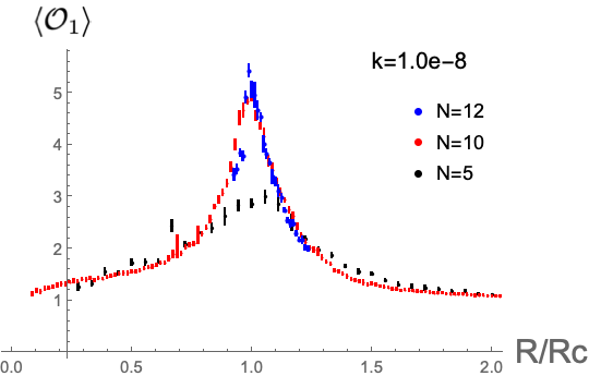
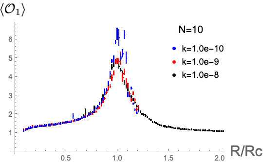
Figure 1: The results of the Monte Carlo simulations for $\langle{\cal O}_{1}\rangle$. The horizontal axes are $R/R_{c}$, where $R_{c}=(N+1)(N+2)/2-N+2$.

Figure 1 shows the results of the Monte Carlo simulations for $\langle{\cal O}_{1}\rangle$. The normalization factor $R_{c}$ for the horizontal axes is chosen as $R_{c}=(N+1)(N+2)/2-N+2$. The perturbative computations in the leading order predict the transition point to be at $R_{c}=(N+1)(N+2)/2$ [15, 16]. However, for the datas shown in the left figure for $k=10^{-8}$, it is better to take $R_{c}=(N+1)(N+2)/2-N+2$ to locate all the peaks near $R/R_{c}=1$. The values of $\langle{\cal O}_{1}\rangle$ approach $1$ as $R$ takes more distant values from $R_{c}$, implying that the correlations become more independent there. On the other hand, the values of $\langle{\cal O}_{1}\rangle$ at the peaks become larger for larger $N$. This can be checked more clearly in Figure 2. This means that the correlation becomes larger at the transition point for larger $N$, which is a typical signature of a continuous phase transition.

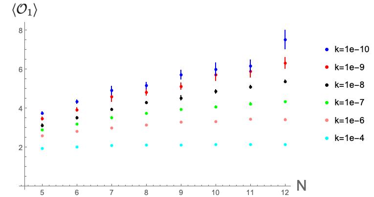
Figure 2: $\langle{\cal O}_{1}\rangle$ from the simulations are plotted against $N$ with $R=(N+1)(N+2)/2-N+2$.

The right picture of Fig. 1 shows the dependence of $\langle{\cal O}_{1}\rangle$ on $k$ for $N=10$. The dependence on $k$ seems little for $R\lesssim R_{c}$, as we will discuss more of this aspect in Section 6.3. On the other hand, at $R\gtrsim R_{c}$, $\langle{\cal O}_{1}\rangle$ seems to become larger as $k$ becomes smaller, slightly shifting the locations of the peaks to the right. This implies that the correlations become larger for smaller $k$ and the critical value $R_{c}$ depends not only on $N$ but also on $k$ as well. The last statement implies that what we have taken as $R_{c}$ above cannot be considered to be a correct expression valid for the general values of the parameters, but can at most be considered to be an approximate expression valid for our parameter range $N\lesssim 12$ and $10^{-10}\lesssim k\lesssim 10^{-8}$.

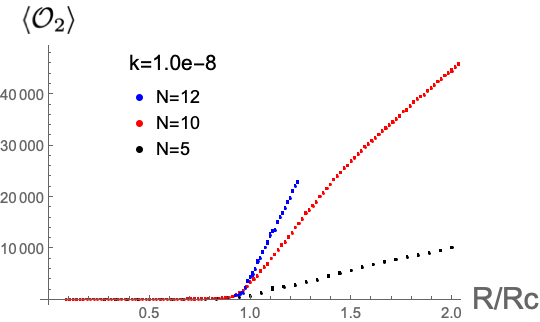
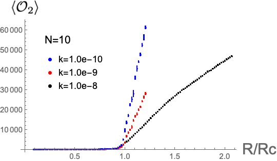
Figure 3: The results of the Monte Carlo simulations for $\langle{\cal O}_{2}\rangle$. The horizontal axes are $R/R_{c}$, where $R_{c}=(N+1)(N+2)/2-N+2$.

Let us next turn to the observable,

$${\cal O}_{2}:=\sum_{i=1}^{R}\phi_{a}^{i}\phi_{a}^{i}=r^{2}.$$ (31)

From the formula (12), by setting the weight $w=2$ and noting ${\cal O}_{2}(\tilde{\phi})=1$ identically, we obtain

$$\langle r^{2}\rangle=\frac{\Gamma\left(\Delta_{NR}+1/3\right)}{\Gamma(\Delta_{NR})}\left\langle\left(\sum_{i,j=1}^{R}\Lambda_{ij}U_{ij}(\tilde{\phi})\right)^{-\frac{1}{3}}\right\rangle$$ (32)

with $\Lambda=\Lambda^{\lambda,k}$. The results of the simulations for $\langle r^{2}\rangle$ are plotted in Figure 3. The figures clearly show that the two phases are characterized by $\langle r^{2}\rangle\sim 0$ for $R<R_{c}$ and $\langle r^{2}\rangle>0$ for $R>R_{c}$, respectively. The transition becomes sharper as $N$ becomes larger or $k$ becomes smaller. $\langle r^{2}\rangle$ changes continuously at $R\sim R_{c}$, supporting the claim that the transition is continuous.

6.2 Comparison with the perturbative computation

In this section, we compare the results of the simulations with the analytic perturbative computation in the leading order, which was reviewed in Section 4. In particular, we see that the analytic computation does not explain the peaks of the correlations of $\tilde{\phi}_{a}^{i}$, which was shown in Section 6.1. We find clear deviations between them around the phase transition point $R\sim R_{c}$, while they converge as $R$ takes distant values from $R_{c}$.

To see this we consider the observables, $U_{d}(\tilde{\phi}):=\sum_{i=1}^{R}U_{ii}(\tilde{\phi})$ and $U_{d}(\phi):=\sum_{i=1}^{R}U_{ii}(\phi)$, whose formulas of the analytic computation are given in (24). The explicit values are obtained by performing the numerical integration of (19) with (18) contained in (24) for $M=1$. On the other hand, we compare these with $\langle U_{d}(\tilde{\phi})\rangle$ and

$$\langle U_{d}(\phi)\rangle=\Delta_{NR}\left\langle\frac{U_{d}(\tilde{\phi})}{\sum_{i,j=1}^{R}\Lambda^{\lambda,k}_{ij}U_{ij}(\tilde{\phi})}\right\rangle$$ (33)

from the simulations, where we have used (12) for $w=6$.

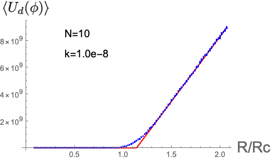
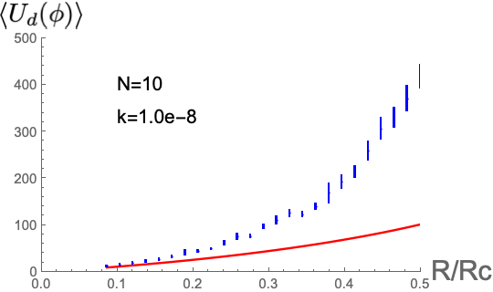
Figure 4: The comparison between the results of the Monte Carlo simulation and the analytic perturbative computation of $\langle U_{d}(\phi)\rangle$ for $N=10$ and $k=10^{-8}$. The blue dots with error bars are the Monte Carlo results, and the red lines are the analytic results. The horizontal axes are $R/R_{c}$, where $R_{c}=(N+1)(N+2)/2-N+2$. The right figure magnifies the region $R/R_{c}<0.5$ in the left figure.

Figure 4 shows the comparison between the Monte Carlo results and the analytic computations. There exist systematic deviations in the vicinity of $R=R_{c}$, as was previously reported in [16]. For $R>R_{c}$, they quickly converge as $R$ leaves $R_{c}$. For $R<R_{c}$, they slowly converge as $R$ becomes smaller.

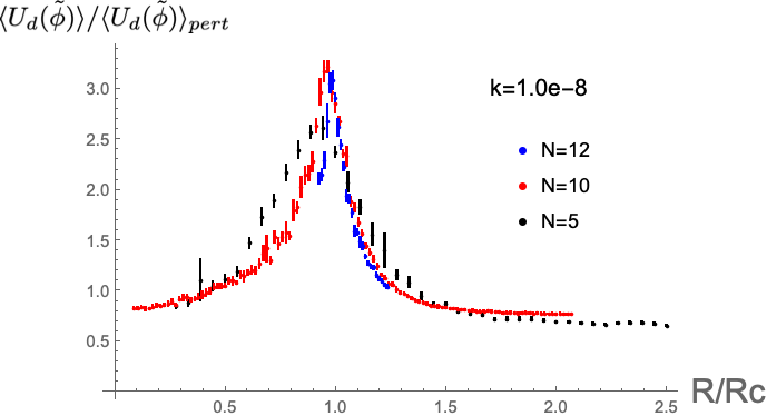
Figure 5: The ratio $\langle U_{d}(\tilde{\phi})\rangle/\langle U_{d}(\tilde{\phi})\rangle_{pert}$ between the Monte Carlo and the perturbative analytic results. The horizontal axes are $R/R_{c}$, where $R_{c}=(N+1)(N+2)/2-N+2$.

One can see similar deviations for the $\langle U_{d}(\tilde{\phi})\rangle$. Figure 5 plots the ratio $\langle U_{d}(\tilde{\phi})\rangle/\langle U_{d}(\tilde{\phi})\rangle_{pert}$ between the Monte Carlo results and the perturbative analytic computations. Indeed the ratio deviates from 1 in the vicinity of the transition point. The deviations at the peaks become larger as $k$ becomes smaller. On the other hand, as shown in Figure 6, it seems that the deviations increase with $N$ for $k<10^{-8}$, but this is not clear for $k\geq 10^{-8}$. We cannot rule out the possibility that they actually converge in the large $N$ limit to some values which increase with the decrease of $k$.

Figure 6: The ratio $\langle U_{d}(\tilde{\phi})\rangle/\langle U_{d}(\tilde{\phi})\rangle_{pert}$ from the simulations are plotted against $N$ with $R=(N+1)(N+2)/2-N+2$.

From the comparisons above, we conclude that the perturbative analytic computation in the leading order does not correctly reproduce the behavior of the matrix model in the vicinity of the transition point. As was previously performed in [16], the situation does not essentially change, even if we take into account the next leading order corrections to the analytic computation.

6.3 $k/\lambda\rightarrow+0$ limit

In this subsection, we focus on the $k/\lambda\rightarrow+0$ limit of the matrix model (1). There are a few reasons to study this. One is the characterization of the phases separated at $R=R_{c}$. We find different limits for each phase at $R>R_{c}$ and $R<R_{c}$. Another is its relevance to the tensor model. The behavior determines whether the wave function is normalizable or not. This will be discussed in Section 7.

Figure 7: The values of $\langle U_{d}(\phi)\rangle$ from the simulations are plotted against $-\log_{10}k$ for $N=10,\ R=45$, which belongs to the region $R<R_{c}$. The reason for a slightly larger error for $k=10^{-8}$ data point may come from the trapping in the narrow region explained in Section 6.6.

Firstly, let us show that the limit $k/\lambda\rightarrow+0$ converges in the phase $R<R_{c}$. This can be seen by looking at the behavior of expectation values of observables. Figure 7 shows the result of the simulation about the behavior of $\langle U_{d}(\phi)\rangle$ in (33) against $k$ for a case with $R<R_{c}$. As can be seen in the figure, the expectation value approaches a constant value in the $k\rightarrow+0$ limit. In fact, similar convergence can be observed also for other observables in other cases with $R<R_{c}$.

Let us discuss the consequence of this behavior to the free energy defined by $F_{N,R}(\lambda,k):=-\log Z_{N,R}(\lambda,k)$. By taking the derivative of (1) with respect to $k$, we obtain

$$\frac{\partial}{\partial k}F_{N,R}(\lambda,k)=\langle U_{d}(\phi)\rangle.$$ (34)

Therefore, as a function of $k$, $F_{N,R}(\lambda,k)$ can be determined by studying the $k$-dependence of $\langle U_{d}(\phi)\rangle$ and performing integration:

$$F_{N,R}(\lambda,k_{1})=\int_{k_{0}}^{k_{1}}dk\,\langle U_{d}(\phi)\rangle+F_{N,R}(\lambda,k_{0}).$$ (35)

In particular, $\lim_{k\rightarrow+0}\langle U_{d}(\phi)\rangle$ will determine $\lim_{k\rightarrow+0}F_{N,R}(\lambda,k)$.

Below let us discuss the behavior of the free energy in $k/\lambda\rightarrow+0$. By performing the rescaling of the variable $\phi_{a}^{i}\rightarrow\lambda^{-1/6}\phi_{a}^{i}$ in (1), one obtains

$$F_{N,R}(\lambda,k)=F_{N,R}(1,k/\lambda)+\frac{NR}{6}\log\lambda.$$ (36)

In the region $R<R_{c}$, there is a finite limit of $\lim_{k\rightarrow+0}\langle U_{d}(\phi)\rangle$ as shown above. Considering (35) and (36), the behavior of the free energy is obtained as

$$F_{N,R}(\lambda,k)=U_{d}^{0}\frac{k}{\lambda}+p_{N,R}(k/\lambda)+\frac{NR}{6}\log\lambda\ \ \hbox{ for }k/\lambda\sim+0\hbox{ and }R<R_{c},$$ (37)

where $U_{d}^{0}:=\lim_{k\rightarrow+0}\langle U_{d}(\phi)\rangle_{\lambda=1}$, and $p_{N,R}(k/\lambda)$ is smaller than $k/\lambda$ in order and has a finite limit $p_{N,R}(+0)$. We comment that this finiteness was proven analytically for $R=2$ and any $N$ previously in [16]. This finiteness of $F_{N,R}(\lambda,k)$ in the $k\rightarrow+0$ limit is non-trivial, as discussed in Section 2.

Figure 8: $k\langle U_{d}(\phi)\rangle$ from the simulations is plotted against $-\log_{10}k$ for $N=10,\ R=80$, which is a case of $R>R_{c}$. The data points can be fitted very well with $k\langle U_{d}(\phi)\rangle\simeq 23.3+107\sqrt{k}$.

On the other hand, for $R>R_{c}$, the simulations show that $\langle U_{d}(\phi)\rangle$ diverges in the $k\rightarrow+0$ limit. An interesting matter is that, instead, $k\langle U_{d}(\phi)\rangle$ converges in the $k\rightarrow+0$ limit, as can be seen from Figure 8. This implies that, from (35), $F_{N,R}(\lambda,k)$ logarithmically diverges in the limit $k/\lambda\rightarrow+0$.

Let us discuss this divergence of the free energy in more detail. As we have seen in Figure 8, if we take $k$ small enough, $k\langle U_{d}(\phi)\rangle$ can be regarded as its limiting value, $\lim_{k\rightarrow+0}k\,\langle U_{d}(\phi)\rangle$. By assuming this for the $N=10$ data in the large $R$ region in the left figure of Figure 4, and fitting a linear function of $R$ for the data in the region $R>1.4\cdot R_{c}$, one obtains,

$$k\,\langle U_{d}(\phi)\rangle|_{k=10^{-8}}\simeq 1.66\cdot(R-65.9).$$ (38)

This curiously agrees very well with what can be obtained by putting $N=10$ to a hypothetical expression for the righthand side,

$$\frac{N}{6}\left(R-\frac{(N+1)(N+2)}{2}\right)=\frac{NR}{6}-\frac{\#P}{2}$$ (39)

where $\#P:=N(N+1)(N+2)/6$ is the number of independent components of a symmetric three-index tensor $P_{abc}$. We have performed similar analyses for $N=5,7$ cases and have found good matches with the hypothesis (39). Assuming the hypothesis and reminding the form (36), we obtain

$$F_{N,R}(\lambda,k)=\tilde{U}_{d}^{0}\log(k/\lambda)+\frac{NR}{6}\log\lambda+\tilde{p}_{N,R}(k/\lambda)\ \ \hbox{ for }k/\lambda\sim+0\hbox{ and }R>R_{c},$$ (40)

where $\tilde{U}_{d}^{0}:=\lim_{k\rightarrow+0}k\,\langle U_{d}(\phi)\rangle$, $\tilde{p}_{N,R}(k/\lambda)$ is smaller than $\log(k/\lambda)$ in order, and

$$\tilde{U}_{d}^{0}=\frac{NR}{6}-\frac{\#P}{2}+\delta\tilde{U}_{d}^{0}$$ (41)

with $\delta\tilde{U}_{d}^{0}$ sub-leading in large $R$. Note that $\tilde{U}_{d}^{0}\geq 0$ due to $\langle U_{d}(\phi)\rangle>0$, and therefore $\delta\tilde{U}_{d}^{0}$ takes positive values in the range $R_{c}<R<(N+1)(N+2)/2$.

Here it is a non-trivial question whether $\tilde{p}_{N,R}(k/\lambda)$ has a finite limit $\tilde{p}_{N,R}(+0)$. For example, a slow correction of order $\sim 1/\log(k)$ to $k\langle U_{d}(\phi)\rangle$ for $k\sim+0$ leads to a double logarithmic divergence of $\tilde{p}_{N,R}(+0)$. However, as shown in Figure 8, the data points of $k\langle U_{d}(\phi)\rangle$ can be fitted very well with a correction of order $\sqrt{k}$, and there is no good motivation for introducing such slow corrections. Therefore it would be reasonable to assume $\tilde{p}_{N,R}(+0)$ to exist as a finite value. We also comment that the hypothesis (39) is nothing but what can be obtained from the perturbative computation in the leading order [15], as the coincidence in the left figure of Figure 4 shows. Therefore $\delta\tilde{U}_{d}^{0}$ is a correction beyond the leading order perturbative computation.

The difference between the behavior of the free energy (37) and (40) characterizes the two phases separated by $R=R_{c}$. These formulas will be used in Section 7.3, where we will discuss the normalizability of the wave function of the tensor model.

6.4 Geometric properties

In Section 6.2, we have found the deviation between the results of the simulations and the perturbative analytic results in the vicinity of the phase transition point. This suggests that some non-perturbative configurations are important in the vicinity of the phase transition point. In this subsection, to discuss the characteristics of the configurations around the phase transition point, we study the distributions of the vectors $\phi_{a}^{i}\ (i=1,2,\ldots,R)$ in the $N$-dimensional vector space associated to the lower index. These vectors define a point cloud with $R$ points, where $\phi^{i}_{a}$ for each $i$ determines the location of each point in the $N$-dimensional vector space. We study the dimensions of such point clouds. It turns out that the dimensions depend on the parameters of the matrix model. In particular, the dimensions take the smallest values at the transition point as functions of $R$.

To study the dimension of a point cloud we use angle distributions among the vectors. The angle between two vectors, say $\phi_{a}^{i}$ and $\phi_{a}^{j}$ $(i\neq j)$, in the $N$-dimensional vector space is given by

$${\rm ang}(\phi^{i},\phi^{j}):=\arccos\left(\frac{\phi_{a}^{i}\phi_{a}^{j}}{\sqrt{\phi_{a}^{i}\phi_{a}^{i}\phi_{b}^{j}\phi_{b}^{j}}}\right).$$ (42)

Assuming that the vectors approximately form a rotationally symmetric $d$-dimensional point cloud, the distribution of the angles should be approximately given by

$$\rho(\theta)\,d\theta={\cal N}\sin^{d-2}(\theta)\,d\theta,$$ (43)

where $\theta$ designates the angle, and ${\cal N}$ is a normalization factor. This formula can easily be obtained by radially projecting points to the unit sphere $S^{d-1}$, and computing infinitesimal areas associated with given mutual angles. The dimensions can be computed by fitting the formula (43) to the angle distributions obtained from the datas.

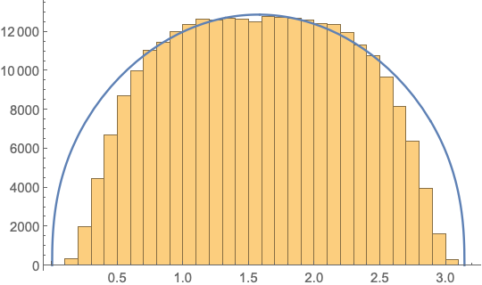
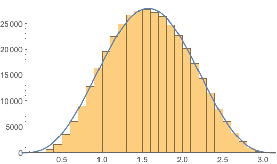
Figure 9: Examples of fitting (43) to the histograms of the mutual angles among $\phi^{i}$s from the actual datas. The horizontal axes represent the angle $\theta$. The parameters are $N=10,\ k=10^{-8}$ with $R=60$ (left) and $R=70$ (right), respectively. Fitting is performed only at the 3/5 portion around the center ($\theta\sim\pi/2$), ignoring 1/5 portions on each side. The fitted values of dimensions are $d=2.4$ and $d=4.7$, respectively, in these cases.

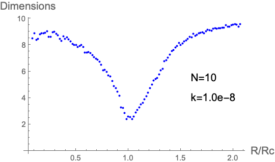
Figure 10: The $R$-dependence of the dimension for $N=10,\ k=10^{-8}$. It takes the lowest value at the transition point. $R_{c}=(N+1)(N+2)/2-N+2$ with $N=10$. Errors are not estimated in this plot.

In Figure 9, we show two examples of the fitting. As shown in the figures, the fitting is generally quite good for high dimensions but not so much for lower dimensions. The reason behind this is that the point clouds cannot be characterised as a single dimensional object but are a mixture of objects with different dimensions, as we discuss in Section 7.2. Yet, to characterize the configurations in terms of dimensions, we perform the fitting restricted to a portion around the center, namely $\theta\sim\pi/2$, because there exist dominant numbers of cases in this region. In this sense, the dimension is merely a qualitative characterization, but it still gives a fairly interesting observable: The dimension takes the lowest value at the phase transition point as a function of $R$. For instance, this can be observed for $N=10,\ k=10^{-8}$ in Figure 10.

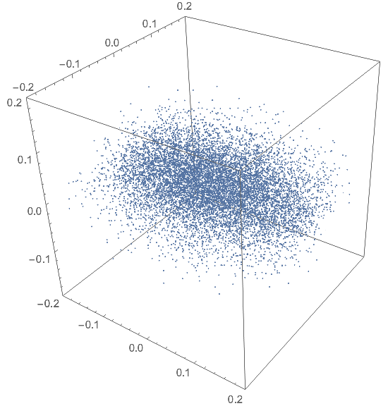
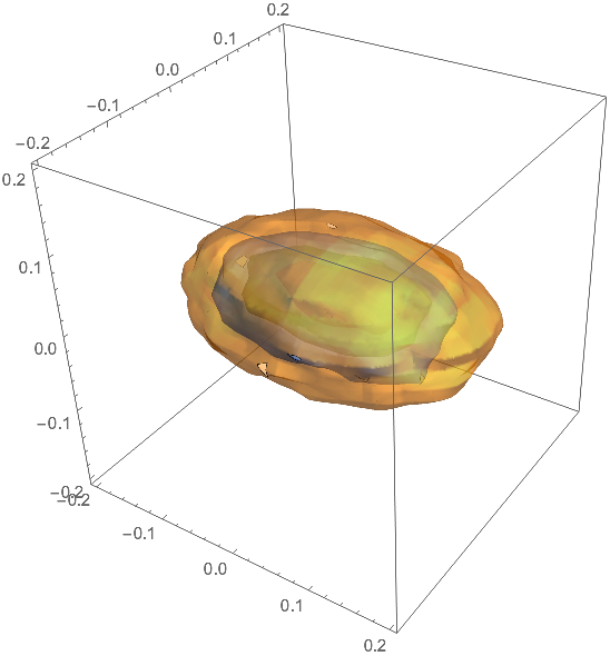
Figure 11: Left: The collection of the point clouds obtained from the simulation with $N=10,\ R=57$, and $k=10^{-8}$. The point cloud from each data of $\phi_{a}^{i}$ is projected into the three-dimensional space and the collection through all the datas are plotted. For the projection, PCA is used to take three major directions out of $N$ dimensions. Right: The corresponding density plot. The shape is like a squashed rugby ball, which may be regarded as an object with a dimension between 2 and 3.

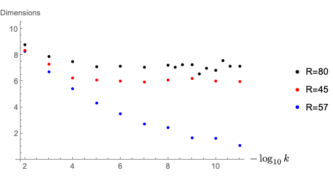
Figure 12: The $k$ dependence of the dimensions of the configurations from the data of $N=10$ and $R$ shown in the figure. The datas for $R=80$ do not converge well for small $k$ due to the difficulty of the simulations explained in Section 6.6. Errors are not estimated in this plot.

It is instructive to directly see a point cloud itself. A point cloud exists in an $N$-dimensional space, but if its dynamical dimension is lower than three, one can project it into a three-dimensional space by extracting the main three extending directions through principal component analysis (PCA). Figure 11 shows a collection of a number of such projected point clouds, which have been sampled from the simulation with $N=10,\ R=57,\ k=10^{-8}$. According to Figure 10, the point cloud has a dimension nearly two in this case, and we indeed find an approximately two-dimensional object which has the shape of a squashed rugby ball as shown in the right figure of Figure 11.

Finally, let us discuss the $k$-dependence of the dimension. The general behavior is that the dimensions decrease with the decrease of $k$ and converge to limiting values, as is shown in Figure 12.

6.5 Symmetry breaking

As shown in Section 6.1, the phase at $R>R_{c}$ is characterized by large values of $\langle r^{2}\rangle$. Since a non-vanishing value of $\phi_{a}^{i}$ breaks the $O(N)$ symmetry associated to the lower index vector space, the phase at $R>R_{c}$ will be characterized by symmetry breaking. In this subsection, we will study this aspect.

Let us consider one of the generators $T_{ab}$ of $SO(N)$. The size of the breaking of $T_{ab}$ by a vector $\phi_{a}^{i}$ will be characterized by the size of the vector $T_{ab}\phi_{b}^{i}$. By considering its square and summing over all the vectors, the breaking by a configuration can be characterized by $\sum_{i=1}^{R}T_{ab}T_{ab^{\prime}}\phi_{b}^{i}\phi_{b^{\prime}}^{i}$. Thus the natural quantity to study is

$$M_{m\,m^{\prime}}:=T^{(m)}{}_{ab}T^{(m^{\prime})}{}_{ab^{\prime}}\sum_{i=1}^{R}\phi_{b}^{i}\phi_{b^{\prime}}^{i},$$ (44)

where $T^{(m)}{}_{ab}\ (m=1,2,\ldots,N(N-1)/2)$ are a basis of the $so(N)$ generators with the normalization $T^{(m)}{}_{ab}T^{(m^{\prime})}{}_{ab}=2\delta_{mm^{\prime}}$ for later convenience. Note that the definition of $M_{m\,m^{\prime}}$ conserves the $S_{R}$ symmetry for the upper index.

An $O(N)$-invariant observable which can be obtained from $M_{m\,m^{\prime}}$ is the set of the eigenvalues of the matrix $M$. For an arbitrary $\phi_{a}^{i}$, we can diagonalize $m_{ab}:=\sum_{i=1}^{R}\phi_{a}^{i}\phi_{b}^{i}$ by an $SO(N)$ transformation. Then it is straightforward to prove that the eigenvalues of $M$ are given by

$$eg(M)=\{e^{\phi}_{a}+e^{\phi}_{b}\,|\,a,b=1,2,\ldots,N,\ a<b\},$$ (45)

where $e^{\phi}_{a}\ (a=1,2,\ldots,N)$ are the eigenvalues of the matrix $m$.

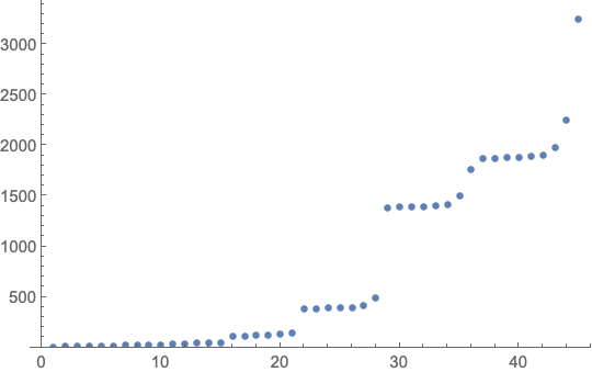
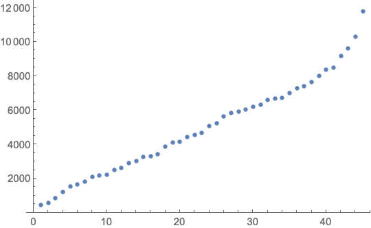
Figure 13: $eg(M)$ defined in (45) are plotted in ascending order for a sample of $\phi_{a}^{i}$, each from a simulation for $R=60$ (left) and for $R=80$ (right), respectively, with $N=10,\ k=10^{-8}$. The stair-like pattern in the left figure implies that the $SO(N)$ symmetry is hierarchically broken to $SO(N-1),\ SO(N-2),\ldots$. In fact, the horizontal locations of the steps agree with the numbers of the generators of $SO(n)\ (n=2,3,\ldots,N)$. All the symmetries are broken with no hierarchal structure in the right figure.

Figure 13 gives two examples of the eigenvalues $eg(M)$. In the figures, the eigenvalues are plotted in ascending order along the horizontal direction. In the case of the left figure, one can find an interesting stair-like pattern of the eigenvalues. This pattern means that the original $SO(N)$ symmetry is hierarchically broken to $SO(N-1),\ SO(N-2),\ldots$. In fact, the horizontal locations of the steps agree with the numbers of the generators of these symmetries. On the other hand, in the case of the right figure, all the symmetries are broken with no obvious hierarchal structure.

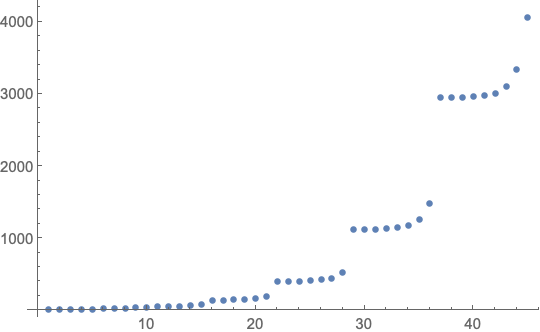
Figure 14: The mean values $\langle eg(M)\rangle$ are plotted for the datas of $R=60$ (left) and of $R=80$ (right), respectively, with $N=10,\ k=10^{-8}$.

Since the pattern above generally fluctuates over the samples of $\phi_{a}^{i}$ in a simulation, we consider an average, $\langle eg(M)\rangle$. The precise definition of this quantity is as follows: we run a simulation with a certain choice of parameters; for each sample of $\phi_{a}^{i}$ in a simulation, we compute eigenvalues $eg(M)$ and order them in ascending order; then we take mean values of each entry over all the datas of the simulation. Figure 14 shows $\langle eg(M)\rangle$ computed from the simulations respectively for $R=60$ (left) and for $R=80$ (right) with $N=10,\ k=10^{-8}$.

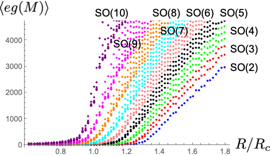
Figure 15: The mean eigenvalues $\langle eg(M)\rangle$ against $R/R_{c}$ for $N=10,\ k=10^{-8}$. $R_{c}=(N+1)(N+2)/2-N+2$. The eigenvalues are plotted vertically at each $R$. For clear distinction, the points are colored according to the numbers of the generators of the symmetries. Each symmetry is broken when the corresponding eigenvalues leave from the horizontal axis.

Figure 15 shows the dependence of $\langle eg(M)\rangle$ over the change of $R$ for $N=10,\ k=10^{-8}$. The eigenvalues start to increase from $R\sim 0.9R_{c}$ with the increase of $R$. The symmetry breaking occurs one by one: first $SO(10)$, then $SO(9)$, and so on, until finally all the symmetries are broken at $R\sim 1.3R_{c}$. In the figure, one can find some gaps between the eigenvalues in the vicinity of $R\sim R_{c}$. They correspond to the differences of the step heights, which for example exist in left figure of Figure 14. As $R$ becomes larger, the gaps gradually disappear, approaching the situation in the right figure of Figure 14.

The above symmetry breaking in a cascade manner is consistent with the results in the previous subsections. When $R<R_{c}$, since $\langle\phi^{2}\rangle$ is small, there is no symmetry breaking. As $R$ increases from $R\sim R_{c}$, the vectors $\phi_{a}^{i}\ (i=1,2,\ldots,R)$ start to take larger values and fill a subspace, the dimension of which increases with the increase of $R$. Since the subspace breaks part of the $SO(N)$ symmetry, depending on its dimensions, more symmetries are broken with the increase of $R$.

Let us comment about the fate of the discrete symmetry $\phi_{a}^{i}\rightarrow-\phi_{a}^{i}\ \forall i$. For $N=\hbox{odd}$, this corresponds to the $Z_{2}$ subgroup of the $O(N)$ symmetry. The quantity, $\sum_{i=1}^{R}\phi_{a}^{i}/R$, is not invariant under the discrete symmetry, and therefore the expectation value of its square, $\langle\sum_{i,j=1}^{R}\phi_{a}^{i}\phi_{a}^{j}\rangle/R^{2}$, will provide a good quantity to measure its breaking. It has turned out that the expectation values computed from the simulation datas stay small in the order $\lesssim O(1)$ over the range, and we have not observed any signatures of its breaking.

6.6 Slowdown of Monte Carlo updates

In the previous work [16], we encountered a rather serious difficulty of the Monte Carlo simulation: For $R\gtrsim R_{c}$ and small $k$, the step sizes of the simulations had to be tuned very small for reasonable acceptance rates of Metropolis updates, but then the updates of configurations were too slow for the system to reach thermodynamic equilibriums within our runtimes. Therefore, in this paper, we have improved the strategy: Integrating out the radial direction of the model and using the so-called Hamiltonian Monte Carlo method for simulations. Indeed the new strategy drastically improves the efficiency of the simulations, but we still encounter the slowdown for smaller $k$, which is however several orders of magnitude smaller than that in the previous work. This implies that this slowdown is an intrinsic property of the model, which is independent from methods of simulations, and would even suggest a possibility of the presence of a transition to a new phase characterized by slow dynamics. However, in this subsection, we will show that the last possibility is unlikely, and the system in the phase at $R>R_{c}$ is rather like a fluid with a viscosity which continuously grows for smaller $k$.

The speed of updates can be quantified by the mean value of distances between neighboring configurations in a sequence of updates, $\tilde{\phi}_{a}^{i}(1),\ \tilde{\phi}_{a}^{i}(2),\ldots,\ \tilde{\phi}_{a}^{i}(M+1)$:

$$\langle(\delta\tilde{\phi})^{2}\rangle:=\frac{1}{M}\sum_{m=1}^{M}\left|\tilde{\phi}(m+1)-\tilde{\phi}(m)\right|^{2},$$ (46)

where $|X|^{2}:=\sum_{i=1}^{R}X_{a}^{i}X_{a}^{i}$. In the ideal maximum situation that each entry of the sequence is independent from the others, $\langle(\delta\tilde{\phi})^{2}\rangle=2$ because of the normalization $|\tilde{\phi}(m)|^{2}=1$.

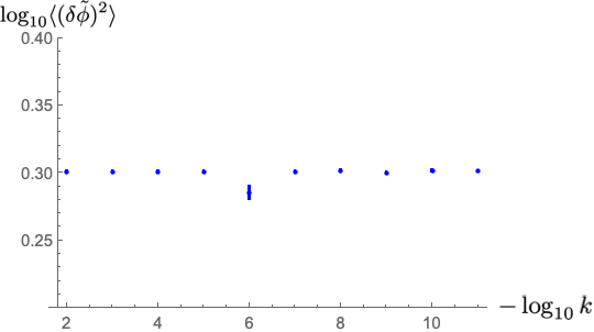
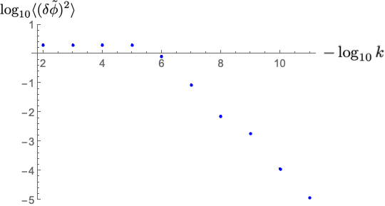
Figure 16: The average speed of updates, $\langle(\delta\tilde{\phi})^{2}\rangle$, is plotted for $R=45$ (left) and $R=80$, respectively, with $N=10$. In the simulations, the ideal maximum situation ($\log_{10}2\sim 0.3$) is realized for $R=45$, while there is a rapid decrease for $R=80$ with the decrease of $k$ for $k\lesssim 10^{-6}$.

Figure 16 shows the dependence of $\langle(\delta\tilde{\phi})^{2}\rangle$ against the value of $k$ for $R=45$ (left) and $R=80$ (right), respectively, with $N=10$. In the simulations, the step sizes, namely the value $\epsilon$ in Section 5, are properly chosen for reasonable acceptance rates for each $k$, while the other parameters of simulations, such as leapfrog numbers, are fixed. The $R=45$ case keeps the ideal values around $\log_{10}2\sim 0.3$ throughout the shown range of $k$. On the other hand, the $R=80$ case has a rapid decrease of the speed with the decrease of $k$ at $k\lesssim 10^{-6}$.

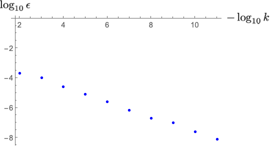
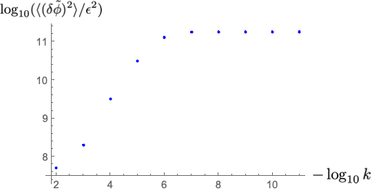
Figure 17: Left: The values of $\epsilon$ for the simulation of $N=10,\ R=80$. Right: The rescaled speed of updates.

The speed of updates defined above is dependent on the parameters of the simulation such as step size, leapfrog number, and even the frequency at which the data is saved, and is therefore not a quantity intrinsic to the model. For instance, the starting point of decreasing, $k\sim 10^{-6}$, has no physical meaning, since this can easily be changed by taking different simulation parameters. However, in the data above, the only parameter which is varied is the step size $\epsilon$ among different values of $k$, and it is therefore meaningful to compare the data for different values of $k$ by rescaling $\langle(\delta\tilde{\phi})^{2}\rangle/\epsilon^{2}$ to cancel the obvious dependence on $\epsilon$. The left figure of Figure 17 plots the values of $\epsilon$ taken for the simulation of $N=10,\ R=80$, and the right is for the corrected values, $\langle(\delta\tilde{\phi})^{2}\rangle/\epsilon^{2}$. In the right figure, leaving aside the irrelevant ideal region $k\gtrsim 10^{-6}$, one can see that the values are almost flat in the region $k\lesssim 10^{-6}$ with no essential change. This implies that the system is basically similar up to the obvious rescaling among different values of $k$.

We also used parallel tempering [33] in addition to the Hamiltonian Monte Carlo method for taking some datas which systematically study $k$-dependencies. The exchanges of configurations were performed among different values of $k$, typically taken $k=10^{-n}\ (n=2,3,\ldots,11)$, with common values of the other parameters. In the region $R>R_{c}$, as $R$ increases from $R_{c}$, the exchange rate quickly reduces for the above choices of $k$’s. Therefore, parallel tempering does not seem effective to solve the slow update problem, which exists at $R\gtrsim R_{c}$ for small $k$. On the other hand, the exchange rate is high for small $k$ at $R\lesssim R_{c}$, which can easily be understood by the presence of the well-defined $k/\lambda\rightarrow+0$ limit at $R<R_{c}$, as discussed in Section 6.3: the sets of configurations are similar among different values of $k$, when $k$ is small enough. However, we did not observe any major differences between the datas with or without parallel tempering. This would imply that there are no major isolated dominant configurations which can only be reached by employing parallel tempering. All in all, we have not observed any essential improvement by employing parallel tempering in addition to the Hamiltonian Monte Carlo method.

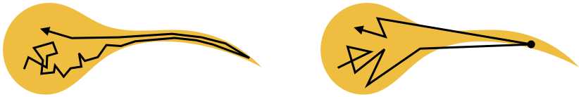
Figure 18: Left: Smooth sampling with relatively smaller $\epsilon$. Sampling smoothly visit both of the broad and narrow regions. Right: Sampling with relatively larger $\epsilon$. Sampling mainly moves within the broad region, but is occasionally trapped for a while in the narrow region.

Another interesting aspect of our actual Hamiltonian Monte Carlo simulation is that a relatively smaller choice of the step size $\epsilon$ seems to give better sampling, and we even took such small values that acceptance rates were nearly 1. This seems to be in contradiction with the more common situation that larger $\epsilon$ with a reasonable acceptance rate like several 10% would give better sampling. However, this apparent contradictory aspect could be explained in the following manner in our case. The positive semi-definite (2) of the first term in the exponent of the matrix model (1) implies that the dominant configurations for small $k$ are around $\sum_{i=1}^{R}\phi_{a}^{i}\phi_{b}^{i}\phi_{c}^{i}\sim 0$, and this condition becomes tighter as $\phi_{a}^{i}$ can take larger values when $k$ is taken smaller. Therefore, the space of dominant configurations can be illustrated as in Figure 18: the dominant configuration space is broad in the small $\phi_{a}^{i}$ region, but it becomes narrower as $\phi_{a}^{i}$ becomes larger. Here, we also assume that dominant configurations are connected, as suggested in the previous paragraph. Assuming the dominant configuration space as shown in the figure, the updates with relatively smaller $\epsilon$ will smoothly visit the narrow region as well as the broad region. On the other hand, sampling with relatively larger $\epsilon$ mainly moves within the broad region, occasionally jumps to the narrow region, and is trapped for a while to compensate the low possibility to visit the narrow region. We have actually observed such trapping to occur more frequently for relatively larger values of $\epsilon$. This occasional trapping damages quality of sampling and it generally takes longer time to obtain a dataset with lower margins of error.

Let us summarize this subsection. We encountered the slowdown of the Monte Carlo updates in the region $R\gtrsim R_{c}$ with small $k$. The speed of updates becomes slower as $k$ becomes smaller, but the dependence is continuous and is subject to the explanation with obvious rescaling. Therefore we have not observed any qualitative changes of the system under the change of the value of $k$, and it is unlikely that there is a phase transition to a new phase with characteristics of slow dynamics. Rather it seems that the system continues to behave like a fluid with a viscosity which continuously grows for smaller $k$ in the region $R\gtrsim R_{c}$.

7 Implications to the tensor model

In this section, we discuss the implications of the results of the simulations to the tensor model in the canonical formalism, the canonical tensor model [23, 24].

7.1 Phase transition point and the consistency of the tensor model

The wave function of the canonical tensor model, that is obtained by solving a number of first-class constraints to the wave function, has the following form [22],

$$\Psi(P)=\left(\int_{\mathbb{R}^{N}}\prod_{a=1}^{N}d\phi_{a}\,\exp\left(I\,P_{abc}\phi_{a}\phi_{b}\phi_{c}\right){\rm Ai}\left(\kappa\,\phi_{a}\phi_{a}\right)\right)^{\frac{\lambda_{H}}{2}},$$ (47)

where $P_{abc}$, a real symmetric tensor, is the configuration variable of the tensor model, $\lambda_{H}=(N+2)(N+3)/2$, $I$ is the imaginary unit (so $I^{2}=-1$), ${\rm Ai}(\cdot)$ designates the Airy Ai function, and $\kappa$ is a real constant in the tensor model. It is particularly important that $\lambda_{H}$ is determined by the hermiticity condition for the Hamiltonian constraint of the tensor model, and therefore must have this particular form depending on $N$. Physically, the sign of the parameter $\kappa$ is supposed to be opposite to that of the cosmological constant, based on the argument relating the mini-superspace approximation of GR and the tensor model with $N=1$ [34] (See an appendix of [16] for more details).

The simplest observable for the physical state represented by the wave function (47) would be given by

$$\begin{split}\langle\Psi|e^{-\alpha\hat{P}_{abc}\hat{P}_{abc}}|\Psi\rangle&=\int_{\mathbb{R}^{\#P}}\prod_{a,b,c=1\atop a\leq b\leq c}^{N}dP_{abc}\,e^{-\alpha P_{abc}P_{abc}}\left|\Psi(P)\right|^{2}\\ &={\cal N}\alpha^{-\#P/2}\int_{\mathbb{R}^{NR}}\prod_{a=1}^{N}\prod_{i=1}^{R}d\phi_{a}^{i}\exp\left(-\frac{1}{4\alpha}\sum_{i,j=1}^{R}U_{ij}(\phi)\right)\prod_{i=1}^{R}{\rm Ai}\left(\kappa\,\phi_{a}^{i}\phi_{a}^{i}\right),\end{split}$$ (48)

where $R=\lambda_{H}$, we have introduced replicas $\phi_{a}^{i}\ (i=1,2,\ldots,\lambda_{H})$ to replace the power coming from that of (47) in the first line, and have performed the Gaussian integration over $P_{abc}$. Here $\alpha$ is an arbitrary positive number, ${\cal N}$ is an unimportant factor independent from $\alpha$, $\#P=N(N+1)(N+2)/6$, i.e. the number of independent components of $P_{abc}$.

The system (48) is complicated due to the presence of the Airy functions. However, when $\kappa$ is taken to be positive, which physically corresponds to a negative cosmological constant, the Airy function ${\rm Ai}\left(\kappa\,\phi_{a}^{i}\phi_{a}^{i}\right)$ is a function that rapidly decays with the increase of $\phi_{a}^{i}\phi_{a}^{i}$. Therefore, as an interesting simplification, we could replace the Airy function by a rapidly damping function with a simpler form. In particular, to make the correspondence to the matrix model (1), we consider a simplified wave function,

$$\Psi_{simple}(P)=\left(\int_{\mathbb{R}^{N}}\prod_{a=1}^{N}d\phi_{a}\,\exp\left(I\,P_{abc}\phi_{a}\phi_{b}\phi_{c}-k(\phi_{a}\phi_{a})^{3}\right)\right)^{\frac{R}{2}}$$ (49)

with $R=\lambda_{H}$ and a positive $k$ by performing the replacement ${\rm Ai}\left(\kappa\,\phi_{a}^{i}\phi_{a}^{i}\right)\rightarrow\exp\left(-k(\phi_{a}^{i}\phi_{a}^{i})^{3}\right)$ in (47). With the observable mentioned above, this leads to

$$\begin{split}\langle\Psi|e^{-\alpha\hat{P}_{abc}\hat{P}_{abc}}|\Psi\rangle&\sim\langle\Psi_{simple}|e^{-\alpha\hat{P}_{abc}\hat{P}_{abc}}|\Psi_{simple}\rangle\\ &=\int_{\mathbb{R}^{\#P}}\prod_{a,b,c=1\atop a\leq b\leq c}^{N}dP_{abc}\,e^{-\alpha P_{abc}P_{abc}}\left|\Psi_{simple}(P)\right|^{2}\\ &={\cal N}\alpha^{-\#P/2}\int_{\mathbb{R}^{NR}}\prod_{a=1}^{N}\prod_{i=1}^{R}d\phi_{a}^{i}\exp\left(-\frac{1}{4\alpha}\sum_{i,j=1}^{R}U_{ij}(\phi)-k\sum_{i=1}^{R}(\phi_{a}^{i}\phi_{a}^{i})^{3}\right)\\ &={\cal N}\alpha^{-\#P/2}Z_{N,R}\left(\frac{1}{4\alpha},k\right),\end{split}$$ (50)

where $R=\lambda_{H}$.

One important matter in the relation (50) between the tensor and matrix models is that the parameter $R$ of the matrix model (1) is related to $N$ by $R=\lambda_{H}=(N+2)(N+3)/2$. What is striking is that this value agrees with the critical value $R_{c}\sim(N+1)(N+2)/2-N+2$ in the leading order of $N$. Considering the ambiguity of the approximate relation (50), we could say that the tensor model is exactly on or at least in the vicinity of (or a little above of) the continuous phase transition point of the matrix model. This is quite intriguing, because our common knowledge tells that continuum theories can often be obtained by taking continuum limits around continuous phase transition points in discretized theories. We could say that the consistency of the tensor model automatically puts the tensor model at the location where a continuum limit may be feasible, though it is currently difficult to conclude this because of the ambiguity contained in the simplification above.

7.2 Dimensions and symmetries of the configurations

In this subsection we will discuss the results of the simulations concerning dimensions and symmetries obtained in Section 6. For this purpose we refer to a property of the wave function (47) that the peaks (ridges) of the wave function are located on the values of $P_{abc}$ which are invariant under Lie-group transformations. This symmetry highlighting phenomenon has been found in [25, 26], where the qualitative argument was given as follows. The integration (47) is of an integrand which oscillates rather widely due to the pure imaginary cubic function in the exponent. Therefore, for a “generic” value of $P_{abc}$, the contributions from different integration spots generally have different phases and mutually cancel among themselves so that the total amount of integration does not take a large value. However, at the location where $P_{abc}$ is invariant under a representation $H$ of a Lie group, $P_{abc}=h_{a}^{a^{\prime}}h_{b}^{b^{\prime}}h_{c}^{c^{\prime}}P_{a^{\prime}b^{\prime}c^{\prime}}\ (\forall h\in H)$, the integration along the gauge orbit $h_{a}^{a^{\prime}}\phi_{a^{\prime}}\ (\forall h\in H)$ contributes coherently in (47), and the wave function has the chance to take a large value compared to that at a “generic” location. This is indeed realized and has concretely been shown for some tractable cases in [25, 26].

The above qualitative argument will hold at least partially after the simplification (49), since we can expect a similar coherence phenomenon in this case, too. Then, from the relation (50), the symmetry highlighting phenomenon of the wave function explained above will have a corresponding phenomenon in the matrix model (1) [16]. Note that this will be valid for general values of $R$, since the constraint $R=\lambda_{H}=(N+2)(N+3)/2$ coming from the consistency of the tensor model has nothing to do with the equalities in (50). In the relation (50), the contribution of a peak with a Lie group representation $H$ in the second line will correspond on the matrix model side to the contributions of $N$-dimensional vectors $\phi_{a}^{i}\ (i=1,2,\ldots,R)$ being distributed along a gauge orbit $h_{a}^{a^{\prime}}\phi_{a^{\prime}}\ (\forall h\in H)$. In the simulation data, such distributed vectors will appear as a point cloud discussed in Section 6.4. This point cloud will have the dimension of the Lie group representation, and will break part of the $SO(N)$ symmetry which is not commutative with $H$. Generally, the wave function contains a number of peaks with various Lie group representations, and therefore the point cloud will be that of a mixture of various gauge orbits. This mixed structure will induce a non-obvious pattern of symmetry breaking, which would be consistent with the hierarchical symmetry breaking in Section 6.5.

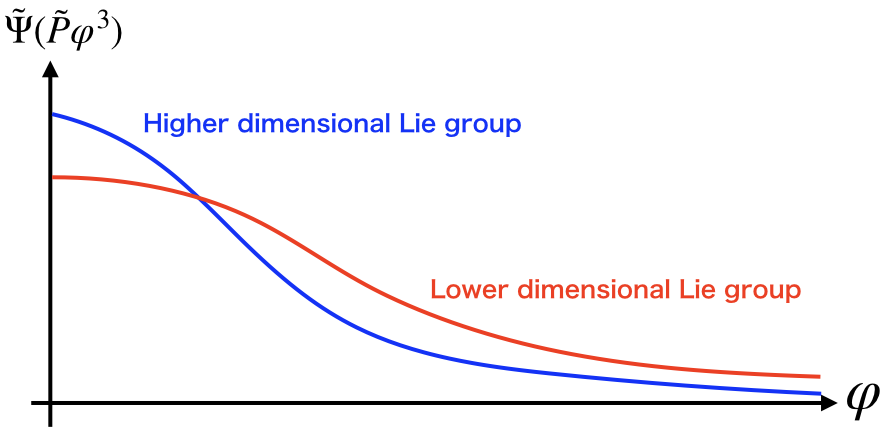
Figure 19: A possible profile of $\tilde{\Psi}(\tilde{P}\varphi^{3})$, depending on the Lie-group symmetry of $\tilde{P}_{abc}$.

To get more information from the behavior obtained in Section 6, let us rewrite the second line in (50) as

$$\begin{split}&\int_{\mathbb{R}^{\#P}}\prod_{a,b,c=1\atop a\leq b\leq c}^{N}dP_{abc}\,e^{-\alpha P_{abc}P_{abc}}\left(\int_{\mathbb{R}^{N}}\prod_{a=1}^{N}d\phi_{a}\,\exp\left(I\,P_{abc}\phi_{a}\phi_{b}\phi_{c}-k(\phi_{a}\phi_{a})^{3}\right)\right)^{R}\\ &={\cal N}\int_{0}^{\infty}dPP^{\#P-NR/3-1}e^{-\alpha P^{2}}\int_{S^{\#P-1}}d\tilde{P}\left(\int_{\mathbb{R}^{N}}\prod_{a=1}^{N}d\varphi_{a}\,\exp\left(I\,\tilde{P}_{abc}\varphi_{a}\varphi_{b}\varphi_{c}-k(\varphi_{a}\varphi_{a})^{3}/P^{2}\right)\right)^{R}\\ &={\cal N^{\prime}}\int_{0}^{\infty}dPP^{\#P-NR/3-1}e^{-\alpha kP^{2}}\int_{S^{\#P-1}}d\tilde{P}\left(\int_{0}^{\infty}d\varphi\,\varphi^{N-1}\ \tilde{\Psi}\left(\tilde{P}\varphi^{3}\right)e^{-\varphi^{6}/P^{2}}\right)^{R},\end{split}$$ (51)

where ${\cal N},\ {\cal N^{\prime}}$ are some unimportant coefficients. Here, to the second line, we have separated $P_{abc}$ into the radial and angular variables, $P_{abc}=P\tilde{P}_{abc}$, where $P=\sqrt{P_{abc}P_{abc}}$, and have introduced a rescaled variable, $\varphi_{a}=P^{1/3}\phi_{a}$. Then, to the last line, we have rescaled $P^{2}\rightarrow kP^{2}$, have divided $\varphi_{a}$ into the radial and angular variables, $\varphi_{a}=\varphi\tilde{\varphi}_{a}$ with $\varphi=\sqrt{\varphi_{a}\varphi_{a}}$, and have introduced

$$\tilde{\Psi}\left(\tilde{P}\varphi^{3}\right):=\int_{S^{N-1}}d\tilde{\varphi}\,e^{I\tilde{P}_{abc}\varphi^{3}\tilde{\varphi}_{a}\tilde{\varphi}_{b}\tilde{\varphi}_{c}}.$$ (52)

The function $\tilde{\Psi}(\tilde{P}\varphi^{3})$ will have a number of peaks at Lie-group symmetric $\tilde{P}_{abc}$. On such a peak, the value of $\tilde{\Psi}(\tilde{P}\varphi^{3})$ will generally become smaller as $\varphi$ increases, because the oscillation of the integrand in (52) will become wilder. In the following paragraphs we will further argue that the $\varphi$-dependence of $\tilde{\Psi}(\tilde{P}\varphi^{3})$ qualitatively depends on the symmetry of $\tilde{P}_{abc}$ as in Figure 19 to explain the dimensional behavior in Figure 10: Namely, for $\tilde{P}_{abc}$ symmetric under higher dimensional Lie-groups, $\tilde{\Psi}(\tilde{P}\varphi^{3})$ takes larger values at small $\varphi$ but quickly decays with $\varphi$, while it takes smaller values at small $\varphi$ but slowly decays with $\varphi$ for $\tilde{P}_{abc}$ symmetric under lower dimensional Lie-groups.

To see how the dimensional behavior in Figure 10 can be explained by the profile in Figure 19, let us first consider $R<(N+1)(N+2)/2$. In this case, the power of $P$ in the integrand of the last line of (51) is positive, and therefore the integral over $P$ will be over the range $0\leq P\lesssim 1/\sqrt{\alpha k}$ with some preference to larger $P$. As $k$ is taken smaller, the larger region of $\varphi$ in the integral of (51) becomes more dominant, making the peaks associated with lower dimensional Lie-groups more dominant than higher dimensional ones. Then the increase of the power $R$ in (51) will enhance the peaks of lower dimensional Lie groups. This explains the decrease of the dimensions with the increase of $R$ in the region $R<R_{c}$ in Figure 10.

Let us next consider $R>(N+1)(N+2)/2$. In this case the power of $P$ in the integrand of (51) is negative, and $P$ will have the preference to smaller values as $R$ increases. Then, the last term in (51) will bound the range of $\varphi$ in the integration, as $R$ increases. Because of the profile in Figure 19, increase of $R$ will enhance the peaks with higher dimensional Lie groups, explaining the increase of dimensions in the region $R>R_{c}$ in Figure 10.

7.3 Normalizability of the wave function of the tensor model

From the physical point of view, it would be interesting to discuss the norm of the wave function of the tensor model. If the wave function of the tensor model successfully represents a spacetime in some manner, the norm of the wave function will linearly diverge in the time direction, which is supposed to form a trajectory in the space of $P_{abc}$. Thus, the normalizability of the wave function has a connection to the question concerning time in the tensor model.

As an approximation or as an example case study similar to the actual case, we discuss the norm of the simplified wave function (49). More precisely, we study the $\alpha\rightarrow+0$ limit of the relation (50):

$$\lim_{\alpha\rightarrow+0}\int_{\mathbb{R}^{\#P}}\prod_{a,b,c=1\atop a\leq b\leq c}^{N}dP_{abc}\,e^{-\alpha P_{abc}P_{abc}}\left|\Psi_{simple}(P)\right|^{2}=\lim_{\alpha\rightarrow+0}{\cal N}\alpha^{-\#P/2}Z_{N,R}\left(\frac{1}{4\alpha},k\right),$$ (53)

where ${\cal N}$ is an unimportant factor independent of $\alpha$.

When $R<R_{c}$, by putting (37) with $\lambda=1/(4\alpha)$ on the righthand side of (53), the dominant $\alpha$ dependence in the $\alpha\rightarrow+0$ limit is obtained as

$$\alpha^{-\#P/2}Z_{N,R}\left(\frac{1}{4\alpha},k\right)\sim\alpha^{NR/6-\#P/2}.$$ (54)

This concludes that the norm diverges for this case by assuming that the critical value satisfies $R_{c}<(N+1)(N+2)/2$.

On the other hand, when $R>R_{c}$, by putting (40) with $\lambda=1/(4\alpha)$ on the righthand side, we obtain

$$\alpha^{-\#P/2}Z_{N,R}\left(\frac{1}{4\alpha},k\right)\sim\alpha^{-\delta\tilde{U}_{d}^{0}},$$ (55)

under the assumption that $\tilde{p}(+0)$ is finite, which has been supported from the data in Section 6.3. This is divergent in the limit $\alpha\rightarrow+0$ in the range $R_{c}<R<(N+1)(N+2)/2$, since $\delta\tilde{U}_{d}^{0}>0$, as discussed in Section 6.3. On the other hand, since $R=\lambda_{H}=(N+2)(N+3)/2$ of the tensor model is in the region $R>(N+1)(N+2)/2$, we cannot currently determine whether the simplified wave function of the tensor model is normalizable or not or how rapidly this diverges if it does. As explained in Section 6.3, this is beyond the leading order perturbative computation.

The simplification (49) of the real wave function (47) is to approximate the case with a positive $\kappa$, which corresponds to a negative cosmological constant. Therefore, it is an interesting future study to determine $\delta\tilde{U}_{d}^{0}$ to answer the physical question concerning the emergence of time in the tensor model for a negative cosmological constant. Note also that the above discussion deals with finite $N$, and therefore taking $N\rightarrow\infty$ would also require more study on this matter.

8 Summary and future prospects

In this paper, we have numerically studied a matrix model with non-pairwise index contractions by Monte Carlo simulations. The matrix model has an intimate connection to the canonical tensor model, a tensor model for quantum gravity in the Hamilton formalism [23, 24], and also has a similar structure as a matrix model that appears in the replica trick of the spherical $p$-spin model ($p=3$) for spin glasses [28, 29]. The matrix model had previously been analyzed by a few analytic methods and Monte Carlo simulations in [15, 16], which had suggested the presence of a continuous phase transition around $R\sim N^{2}/2$. This relation between $N$ and $R$ is particularly interesting, because this agrees with a consistency condition of the tensor model in the leading order of $N$, implying that the tensor model is automatically located exactly on or near a continuous phase transition point. However, in the previous works the evidence for the phase transition was not very clear. In this paper we have presented a new set up for Monte Carlo simulations by first integrating out the radial direction, and have studied the model by employing the more efficient Hamiltonian Monte Carlo method. We have obtained considerable improvement of the efficiency of the simulations, and have found a rather sharp continuous phase transition around $R=R_{c}\sim(N+1)(N+2)/2-N+2$. We have also studied various properties of the phase transition and the two phases: the dimensions of the configurations take the smallest values at the transition point; the phase at $R>R_{c}$ is characterized by cascade symmetry breaking; and the $k/\lambda\rightarrow+0$ limit is convergent in one phase and diverges in the other.

We have also discussed some implications to the tensor model. In particular, the most striking is the coincidence above between the location of the continuous phase transition point and the consistency condition of the tensor model in the leading order of $N$. A well known fact is that continuum theories can often be obtained by taking a continuum limit near a continuous phase transition point. This means that the tensor model seems to automatically put itself at the location where it is possible to find a sensible continuum limit. We have also discussed the wave function of the tensor model by using the connection between the matrix model and an approximation of a known exact wave function of the tensor model. In particular, we have provided a qualitative argument for the dependence on $R$ of both the dimension of the preferred class of configurations and the observed symmetry breaking patterns, using the intimate connection between Lie-group symmetries and peaks of the wave function as has been investigated before [25, 26].

While we have numerically obtained a rather clear picture of the phase structure of the matrix model, we are still seriously lacking analytic understanding. As shown in Section 6.2, there seem to exist essential differences between the numerical results and the analytic perturbative results performed in [15, 16]. Moreover, other than the qualitative argument given in Section 7.2, a more rigorous understanding of the behavior of the dimensions and the symmetry breaking would be desirable. Analytic understanding is also necessary to discuss the continuum limit discussed in the previous paragraph, since taking a large $N$ limit while simultaneously tuning $R$ and $k$ is difficult to do exclusively through numerical methods. Developing an analytical non-perturbative understanding is an important future direction to understand the dynamics of the matrix model.

Though this paper has given several clear pieces of evidence for the phase transition in the matrix model, explaining its interesting connection to the canonical tensor model, various things still need to be explored in order to understand more about the canonical tensor model through matrix models of the similar sort. Most importantly, the simplification of the wave function discussed in Section 7.1 by approximating the Airy function for $\kappa>0$ by a conveniently chosen damping function does not explain whether the obtained results are universal under a different choice of a damping function. Moreover, from a physical point of view we would like to explore the $\kappa<0$ case corresponding to the positive cosmological constant, rather than the $\kappa>0$ case corresponding to the negative cosmological constant. In the case of $\kappa<0$, the Airy function becomes oscillatory, and the dynamics will most likely be different from the $\kappa>0$ case. Since this case suffers from the notorious sign problem, it is technically very challenging. It would also be an interesting future direction to apply new Monte Carlo methods developed to analyze various other systems suffering from sign problems to our case, as well as to develop analytical treatment.

References

- [1] M. Reuter and F. Saueressig, “Quantum Gravity and the Functional Renormalization Group : The Road towards Asymptotic Safety,” Cambridge University Press, 2019.
- [2] R. Loll, “Quantum Gravity from Causal Dynamical Triangulations: A Review,” arXiv:1905.08669 [hep-th].
- [3] C. Rovelli and F. Vidotto, “Covariant Loop Quantum Gravity : An Elementary Introduction to Quantum Gravity and Spinfoam Theory,” Cambridge University Press, 2014.
- [4] S. Surya, “The causal set approach to quantum gravity,” arXiv:1903.11544 [gr-qc].
- [5] T. Konopka, F. Markopoulou and L. Smolin, “Quantum Graphity,” hep-th/0611197.
- [6] E. Wigner, “Characteristic vectors of bordered matrices with infinite dimensions”, Annals of Mathematics 62 (3): 548-564.
- [7] G. ’t Hooft, “A planar diagram theory for strong interactions,” Nucl. Phys. B 72, 461 (1974).
- [8] E. Brezin and V. A. Kazakov, “Exactly Solvable Field Theories of Closed Strings,” Phys. Lett. B 236, 144 (1990). doi:10.1016/0370-2693(90)90818-Q
- [9] M. R. Douglas and S. H. Shenker, “Strings in Less Than One-Dimension,” Nucl. Phys. B 335, 635 (1990). doi:10.1016/0550-3213(90)90522-F
- [10] D. J. Gross and A. A. Migdal, “Nonperturbative Two-Dimensional Quantum Gravity,” Phys. Rev. Lett. 64, 127 (1990). doi:10.1103/PhysRevLett.64.127
- [11] J. Ambjorn, B. Durhuus, and T. Jonsson, “Three-dimensional simplicial quantum gravity and generalized matrix models,” Mod. Phys. Lett. A06 (1991) 1133–1146.
- [12] N. Sasakura, “Tensor model for gravity and orientability of manifold,” Mod. Phys. Lett. A06 (1991) 2613–2624.
- [13] N. Godfrey and M. Gross, “Simplicial quantum gravity in more than two-dimensions,” Phys. Rev. D43 (1991) R1749–1753.
- [14] R. Gurau, “Colored Group Field Theory,” Commun. Math. Phys. 304, 69 (2011) doi:10.1007/s00220-011-1226-9 [arXiv:0907.2582 [hep-th]].
- [15] L. Lionni and N. Sasakura, “A random matrix model with non-pairwise contracted indices,” PTEP 2019, no. 7, 073A01 (2019) doi:10.1093/ptep/ptz057 [arXiv:1903.05944 [hep-th]].
- [16] N. Sasakura and S. Takeuchi, “Numerical and analytical analyses of a matrix model with non-pairwise contracted indices,” Eur. Phys. J. C 80, no. 2, 118 (2020) doi:10.1140/epjc/s10052-019-7591-9 [arXiv:1907.06137 [hep-th]].
- [17] A. Anderson, R. C. Myers and V. Periwal, “Complex random surfaces,” Phys. Lett. B 254, 89 (1991).
- [18] A. Anderson, R. C. Myers and V. Periwal, “Branched polymers from a double scaling limit of matrix models,” Nucl. Phys. B 360, 463 (1991).
- [19] R. C. Myers and V. Periwal, “From polymers to quantum gravity: Triple scaling in rectangular random matrix models,” Nucl. Phys. B 390, 716 (1993) [hep-th/9112037].
- [20] S. Nishigaki and T. Yoneya, “A nonperturbative theory of randomly branching chains,” Nucl. Phys. B 348, 787 (1991). doi:10.1016/0550-3213(91)90215-J
- [21] P. Di Vecchia, M. Kato and N. Ohta, “Double scaling limit in O(N) vector models in D-dimensions,” Int. J. Mod. Phys. A 7, 1391 (1992). doi:10.1142/S0217751X92000612
- [22] G. Narain, N. Sasakura and Y. Sato, “Physical states in the canonical tensor model from the perspective of random tensor networks,” JHEP 1501, 010 (2015) doi:10.1007/JHEP01(2015)010 [arXiv:1410.2683 [hep-th]].
- [23] N. Sasakura, “Canonical tensor models with local time,” Int. J. Mod. Phys. A 27, 1250020 (2012) doi:10.1142/S0217751X12500200 [arXiv:1111.2790 [hep-th]].
- [24] N. Sasakura, “Uniqueness of canonical tensor model with local time,” Int. J. Mod. Phys. A 27, 1250096 (2012) doi:10.1142/S0217751X12500960 [arXiv:1203.0421 [hep-th]].
- [25] D. Obster and N. Sasakura, “Emergent symmetries in the canonical tensor model,” PTEP 2018, no. 4, 043A01 (2018) doi:10.1093/ptep/pty038 [arXiv:1710.07449 [hep-th]].
- [26] D. Obster and N. Sasakura, “Symmetric configurations highlighted by collective quantum coherence,” Eur. Phys. J. C 77, no. 11, 783 (2017) doi:10.1140/epjc/s10052-017-5355-y [arXiv:1704.02113 [hep-th]].
- [27] T. Kawano, D. Obster and N. Sasakura, “Canonical tensor model through data analysis: Dimensions, topologies, and geometries,” Phys. Rev. D 97, no. 12, 124061 (2018) doi:10.1103/PhysRevD.97.124061 [arXiv:1805.04800 [hep-th]].
- [28] A. Crisanti and H.-J. Sommers, “The spherical p-spin interaction spin glass model: the statics,” Z. Phys. B 87, 341 (1992).
- [29] T. Castellani and A. Cavagna, “Spin-glass theory for pedestrians”, J. Stat. Mech.: Theo. Exp. 2005, 05012 [arXiv: cond-mat/0505032].
- [30] R. M. Neal, “MCMC using Hamiltonian dynamics,” in The Handbook of Markov Chain Monte Carlo, Brooks S, Gelman A, Jones G L, and Meng X L (eds.) Chapman & Hall, CRC Press, 113 (2010) [arXiv:1206.1901 [stat.CO]].
- [31] S. Byrne and M. Girolami. “Geodesic Monte Carlo on Embedded Manifolds,” Scandinavian Journal of Statistics 40.4 (2013): 825-845.
- [32] M. Hanada, “Markov Chain Monte Carlo for Dummies,” arXiv:1808.08490 [hep-th].
- [33] D. J. Earl, and M. W. Deem, “Parallel Tempering: Theory, Applications, and New Perspectives,” Physical Chemistry Chemical Physics 7.23 (2005): 3910.
- [34] N. Sasakura and Y. Sato, “Interpreting canonical tensor model in minisuperspace,” Phys. Lett. B 732, 32 (2014) doi:10.1016/j.physletb.2014.03.006 [arXiv:1401.2062 [hep-th]].