Bootstraps Regularize Singular Correlation Matrices

Abstract

I show analytically that the average of $k$ bootstrapped correlation matrices rapidly becomes positive-definite as $k$ increases, which provides a simple approach to regularize singular Pearson correlation matrices. If $n$ is the number of objects and $t$ the number of features, the averaged correlation matrix is almost surely positive-definite if $k>\frac{e}{e-1}\frac{n}{t}\simeq 1.58\frac{n}{t}$ in the limit of large $t$ and $n$. The probability of obtaining a positive-definite correlation matrix with $k$ bootstraps is also derived for finite $n$ and $t$. Finally, I demonstrate that the number of required bootstraps is always smaller than $n$. This method is particularly relevant in fields where $n$ is orders of magnitude larger than the size of data points $t$, e.g., in finance, genetics, social science, or image processing.

Keywords Correlation  $\cdot$ Regularization  $\cdot$ High-Dimensionality

1 Introduction

Correlation and covariance matrices are fundamental dependence estimators in statistical inference. Their use includes risk minimization in finance [1], analysis of functional genomics [2], or image processing [3]. However, when the number of objects under study ($n$) exceeds the number of available data points ($t$), theses matrices cannot be inverted. As a result, many standard inference methods cannot be applied directly. To overcome this issue, a large literature on eigenvalue regularization has been devoted to this issue over the last decades. The most relevant ones are the Ledoit-Wolf linear shrinkage [4] and the more recent non-linear shrinkage [5]. These methods, apart from regularizing singular correlation matrices, attempt to reduce the noise effect due to finite sample size. In addition, Ref. [6] proposes a recursive algorithm that aims to find the most similar positive-definite matrix to an initial problematic matrix that is not positive-definite. Similarly to the proposed method, this approach does not try to denoise the target matrix but corrects the eigenvalue distribution by removing the non-positive eigenvalues.

In this work, I propose a simple alternative approach based on bootstrap resampling to regularize correlation matrices with $z>0$ zero degenerate eigenvalues. In particular, I prove that the probability to obtain a positive defined matrix from the average of $k$ bootstrap resampling scenarios converges rapidly with respect to $k$ to one provided that $k$ is larger than $\frac{e}{e-1}\frac{n}{t}$.

2 The Bootstrap Average Correlation Matrix

Let $\textbf{X}\in\mathbb{R}^{n\times t}$ be the data matrix and $\textbf{C}\in\mathbb{R}^{n\times n}$ its Pearson correlation matrix. We assume that no column or row of X is a linear combination of the others; this implies that C has rank $r=\min\{n,t-1\}$. Let $\textbf{X}^{(b)}\in\mathbb{R}^{n\times t}$ be a bootstrap copy of X obtained by sample replacement of the columns of X, and $\textbf{C}^{(b)}$ its correlation matrix. A generic element of $\textbf{X}^{(b)}$ is $x^{(b)}_{ij}=x_{ih^{(b)}_{j}}$, where ${\bf{h}}^{(b)}$ is a vector of dimension $t$ obtained by random sampling with replacement of the elements of vector $(1,2,\cdots,t)$.

This paper derives an approximate expression of the probability that the smallest eigenvalue $\lambda_{0}$ of the correlation matrix $\langle\textbf{C}\rangle:=k^{-1}\sum_{i=0}^{k}\textbf{C}^{(i)}$ is larger than zero as a function of the number of bootstrap copies. The minimum number of bootstrap copies $k^{+}$, that guarantees $\langle\textbf{C}\rangle$ to be positive-definite within a chosen confidence level, shows a real transition in the large-system limit, defined here as $n,t\to\infty$ at fixed $q$.

3 The Distribution of the Number of Null Eigenvalues

The first step is to obtain a probability distribution of the number of zero eigenvalues $z_{b}$ of a given bootstrap correlation matrix $\textbf{C}^{(b)}$. One has

$$z_{b}=\max\{n+1-u_{b},\,0\},$$ (1)

where $u_{b}$ is the number of unique column indices sampled from X in the $b$-bootstrap copy. The exact probability distribution of $u_{b}$ is known to be [7]

$$\mathcal{P}(u_{b})=\frac{\mathcal{S}_{2}(t,u_{b})\,t!}{t^{t}\,(t-u_{b})!}$$ (2)

where $\mathcal{S}_{2}(t,u_{b})$ is the Sterling number of the second kind. Such a distribution has mean and variance

$$\left.\begin{aligned} \mu(t)&=t\,\left[1-\left(1-\frac{1}{t}\right)^{t}\right]\\ \sigma^{2}(t)&=t\,\left(1-\frac{1}{t}\right)^{t}+t^{2}\,\left(1-\frac{1}{t}\right)\left(1-\frac{2}{t}\right)^{t}-t^{2}\,\left(1-\frac{1}{t}\right)^{2t}.\end{aligned}\right.$$ (3)

In the limit of large $t$, eqs (3) become

$$\left.\begin{aligned} \mu(t)&\approx\left(1-\frac{1}{e}\right)t+\frac{1}{2e}\\ \sigma^{2}(t)&\approx\left(\frac{e-2}{e^{2}}\right)t+\frac{3-e}{2e^{2}}\,.\end{aligned}\right.$$ (4)

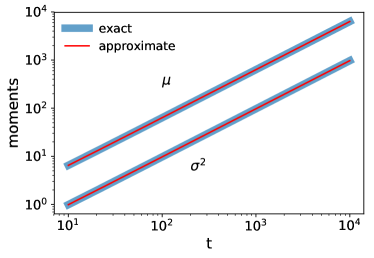
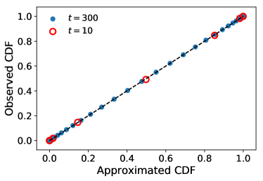
Figure 1: The left plot shows the exact (Eq. (3)) and approximate (eq. (4)) $t$-dependence of the first two moments of $\mathcal{P}(u_{b})$ distribution of Eq. (2). The right plot shows the approximate Normal Cumulative Distribution Function (CDF) against the observed CDF obtained with $10^{4}$ random sampling for every integer value of $u_{b}\in[0,t]$.

Furthermore, it is worth noticing that the deviation of the empirical $\mathcal{P}(u_{b})$ from a normal $\mathcal{N}(\mu(t),\sigma(t))$ is negligible for even for moderately large $t$ [7] , as reported in the right-hand side plot of Fig. 1.

If we consider a condition characterized by an abundance of expected zero eigenvalues, i.e., $n\gg t$, then the probability distribution of $z_{b}$ according to Eq. (1) can be approximate by a Normal distribution

$$\mathcal{P}(z_{b})\approx\mathcal{N}\left(n+1-\mu(t),\sigma(t)\right)\,.$$ (5)

Now that the distribution of the zero eigenvalues for the single bootstrap copy is known, we can answer the original question, and consider $k$ bootstrap copies of X such that $\langle\textbf{C}\rangle:=k^{-1}\sum_{i=1}^{k}\textbf{C}^{(i)}$.

To make further progress, it is necessary to recall the geometrical properties of the space associated to degenerate eigenvalues. Let us suppose that $\textbf{C}^{(i)}$ has $z_{i}$ zero eigenvalues. Then the set of eigenvectors associated with these zero eigenvalues defines a hyper-plane $V_{i}$ of dimension $z_{i}$ embedded in an $n$ dimensional space. Each vector w that lies in $V_{i}$ verifies $\textbf{w}\,\textbf{C}^{(i)}\,\textbf{w}^{\prime}=0$; however, if there is at least another $j\neq i$ whose $z_{j}$ zero eigenvalues of $\textbf{C}^{(j)}$ define hyper-plane $V_{j}$ such that $\mbox{dim}(V_{i}\cap V_{j})\ngeq 1$, then $\textbf{w}\,\textbf{C}^{(j)}\,\textbf{w}^{\prime}>0$; and thus $\textbf{w}\,\langle\textbf{C}\rangle\,\textbf{w}^{\prime}>0$ for every vector w that lies in $V_{i}$ or $V_{j}$.

It is important to point out that eigenvectors associated to $z_{i}$ zero eigenvalues can be assumed to be “randomly” chosen with the constraint to be orthogonal with $V_{i}^{\perp}$, the space defined by the eigenvectors associated with the $n-z_{i}$ non-zero eigenvalues; this because they do not carry any information about the correlation matrix $\textbf{C}^{(i)}$ since they explain zero variance. Therefore every rotation of the basis of $V_{i}$ constrained to be orthogonal with $V_{i}^{\perp}$ will produce exactly the same matrix $\textbf{C}^{(i)}$. In the $k=2$ case, the probability that $\mbox{dim}(V_{1}\cap V_{2})\ngeq 1$ will be approximately $1$ if $z_{1}+z_{2}\leq n$ and $0$ otherwise. It is possible to visualize this relationship easily in a three-dimensional space, i.e., $n=3$. In case of two random straight lines, that have dimensions $z_{1}=1$ and $z_{2}=1$, the probability that they intersect in a straight line is almost zero since they must be coincident; differently, if we consider two random planes $z_{1}=2$ and $z_{2}=2$ they will intersect in a straight line almost surely apart from only configurations in which they are parallels. The above-discussed approximation, in the case of the spectral decomposition, is valid if the probability that the orthogonal spaces $V_{1}^{\perp}$ and $V_{2}^{\perp}$ defined from the $n-z_{1}$ and $n-z_{2}$ non-zero eigenvalues perfectly overlap is negligible. In a bootstrap resampling, when $t$ is sufficiently large, this probability is approximately zero, as this requires to sample the same column indices of X for both bootstrap realizations, in other words, $\textbf{C}^{(1)}=\textbf{C}^{(2)}$.

More generally, for $k$ bootstrap copies, every hyper-plane $V_{i}$ will verify $\mbox{dim}(V_{i}\cap V_{j})\ngeq 1$ for at least one $j\neq i$ with probability $1$ if

$$\zeta:=\sum_{i=1}^{k}z_{i}\leq(k-1)\,n.$$ (6)

If the above inequality holds, then $\langle\textbf{C}\rangle$ has no zero eigenvalue. From Eq. (6), one can derive an upper bound for the number of bootstrap copies required. In fact, even if all bootstrap correlations have $n-1$ null eigenvalues, no more than $k=n$ bootstrap copies are necessary to obtain a positive define matrix $\langle\textbf{C}\rangle$.

According to Eq. (5), the distribution of $\zeta$ can be approximated by a sum of $k$ identical normal distributions that converges to

$$\mathcal{P}(\zeta)\approx\mathcal{N}\left(k\,(n+1-\mu(t)),\sqrt{k}\,\sigma(t)\right).$$ (7)

Therefore, the probability that the smallest eigenvalue $\lambda_{0}$ of $\langle\textbf{C}\rangle$ is larger than zero can be obtained from the cumulative distribution function of $\mathcal{P}(\zeta)$ estimated at $(k-1)\,n$, that is

$$\mathcal{P}(\lambda_{0}>0)\approx\mathcal{P}\left(\zeta\leq(k-1)\,n\right)=\int^{(k-1)\,n}_{-\infty}\mathcal{P}(\zeta)\,d\zeta\approx\frac{1}{2}\left[1+\mbox{erf}\left(\frac{[\mu(t)-1]\,k-n}{\sigma(t)\,\sqrt{2k}}\right)\right]$$ (8)

The above equation suggests to set a threshold $\alpha$ such that $\mathcal{P}(\lambda_{0}>0)>1-\alpha$, i.e. $1-\mbox{erf}(a)=\alpha$ (for example, $a\approx 1.82$ for $\alpha=0.01$). One can then define the number of bootstraps required to achieve $\mathcal{P}(\lambda_{0}>0)>1-\alpha$ by setting the argument of the erf function to $a$, which gives

$$k^{+}(a)\simeq\frac{a^{2}\sigma^{2}(t)+[\mu(t)-1]n+\sqrt{a^{4}\sigma^{4}(t)+2a^{2}\sigma^{2}(t)[\mu(t)-1]n}}{[\mu(t)-1]^{2}}$$ (9)

A bi-dimensional mapping of the values of $k^{+}(a)$ with $a=1.82$ as function of $n$ and $t$, shown in Fig. 2 left, shows that the number of bootstrap copies $k^{+}$ required to have a positive defined $\langle\textbf{C}\rangle$ is quite small, at least for not too extreme values of $q=n/t$.

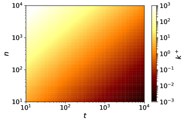
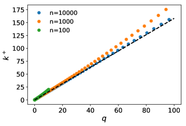
Figure 2: The left plot shows a color map of the analytical value of $k^{+}(a)$, with $a=1.82$, for different $n$ and $t$. The right plot shows the analytical (dots) and large-system limit (dotted line) values of $k^{+}$ obtained for $t$ that span a geometric progression range in $[10,10^{4}]$ such that $q\in[1,100]$. The large-system limit is obtained from Eq.(12).

To have a rough estimate of the transition point $k^{+}$ for $\mathcal{P}(\lambda_{0}>0)\approx 1$ in the limit of large $n$, we can substitute $t=n/q$, and compute the $k^{*}$ of the inflection point of the error function, obtained for the argument of erf equals to zero

$$k^{*}=\frac{2enq}{2(e-1)n+(1-2e)q}\,.$$ (10)

The large-system limit of the first derivative slope at the inflection point if the error function diverges to infinity

$$\lim_{n\to\infty}\frac{d}{dk}\,\left.\frac{k\left[2(e-1)n-2eq+q\right]-2enq}{2q\sqrt{k\left[\frac{2(e-2)n}{q}-e+3\right]}}\right|_{k=k^{*}}=\infty\,.$$ (11)

This means that $\mathcal{P}(\lambda_{0}>0)$ has a real transition in the large-system limit. The value of the inflection point of Eq. (10), in the large-system limit, converges to

$$\lim_{n\to\infty}k^{*}=\lim_{n\to\infty}k^{+}(a)=\frac{e}{(1-e)}q\approx 1.58\frac{n}{t}$$ (12)

The right-hand side of Fig. 2 shows that this approximation can provide a quite accurate estimation of the magnitude of $k^{+}$ even for $n$ small when $q$ is not extremely large.

In summary, both the approximate distribution of $\mathcal{P}(\lambda_{0}>0)$ of Eq. (8) and the bound limits $k^{+}$ of Eqs. (9) show a very good agreement with the observations, reported in Fig. 3.

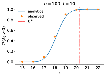
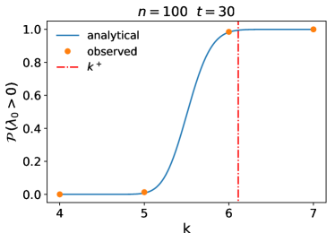
Figure 3: Observed and predicted probability that $\langle\textbf{C}\rangle$ has no zero eigenvalues with $k$ bootstrap copies, for various $n$ and $t$. The figure shows the predicted $k^{+}(a)$ limit, with $a=1.82$. The simulations are obtained by sampling X from a standardized multivariate normal distribution.

4 Discussion

I have shown that the average correlation matrix of $k$ bootstrap copies converges to a positive-defined matrix for $k$ much smaller than the order of the matrix. Such a matrix can be used in many applications which require to invert $C$, such as risk optimization. An extensive comparative analysis of the performance of these approaches will be addressed in future works.

References

References

- [1] Harry Markowitz. Portfolio selection: Efficient diversification of investments, volume 16. John Wiley New York, 1959.
- [2] Juliane Schäfer and Korbinian Strimmer. A shrinkage approach to large-scale covariance matrix estimation and implications for functional genomics. Statistical Applications in Genetics and Molecular Biology, 4(1), 2005.
- [3] Santiago Velasco-Forero, Marcus Chen, Alvina Goh, and Sze Kim Pang. Comparative analysis of covariance matrix estimation for anomaly detection in hyperspectral images. IEEE Journal of Selected Topics in Signal Processing, 9(6):1061–1073, 2015.
- [4] Olivier Ledoit and Michael Wolf. A well-conditioned estimator for large-dimensional covariance matrices. Journal of Multivariate Analysis, 88(2):365–411, 2004.
- [5] Olivier Ledoit and Michael Wolf. Nonlinear shrinkage of the covariance matrix for portfolio selection: Markowitz meets goldilocks. The Review of Financial Studies, 30(12):4349–4388, 2017.
- [6] Nicholas J Higham. Computing the nearest correlation matrix—a problem from finance. IMA Journal of Numerical Analysis, 22(3):329–343, 2002.
- [7] Alex F Mendelson, Maria A Zuluaga, Brian F Hutton, and Sébastien Ourselin. What is the distribution of the number of unique original items in a bootstrap sample? arXiv preprint arXiv:1602.05822, 2016.