Computing Local Sensitivities of Counting Queries with Joins

Abstract

Local sensitivity of a query Q given a database instance D, i.e. how much the output Q(D) changes when a tuple is added to D or deleted from D, has many applications including query analysis, outlier detection, and in differential privacy. However, it is NP-hard to find local sensitivity of a conjunctive query in terms of the size of the query, even for the class of acyclic queries. Although the complexity is polynomial when the query size is fixed, the naive algorithms are not efficient for large databases and queries involving multiple joins. In this paper, we present a novel approach to compute local sensitivity of counting queries involving join operations by tracking and summarizing tuple sensitivities – the maximum change a tuple can cause in the query result when it is added or removed. We give algorithms for the sensitivity problem for full acyclic join queries using join trees, that run in polynomial time in both the size of the database and query for an interesting sub-class of queries, which we call ‘doubly acyclic queries’ that include path queries, and in polynomial time in combined complexity when the maximum degree in the join tree is bounded. Our algorithms can be extended to certain non-acyclic queries using generalized hypertree decompositions. We evaluate our approach experimentally, and show applications of our algorithms to obtain better results for differential privacy by orders of magnitude.

1 Introduction

Understanding how adding or removing a tuple to the relations in the database affects the query output is an important task to many applications [28, 35, 30]. For instance, airline companies need to search for a new flight that can meet the requirements of popular trips. Sales companies should identify the critical part in the production to minimize the number of orders affected by this part. Besides these examples for query explanations, applications of the state-of-the-art privacy guarantee – differential privacy [20] – also need to add sufficient amount of noise to hide the change in the query output due to adding or removing a tuple. In particular, given a database instance $\mathcal{D}$, the maximum change to the query output when one of the given tables in the database adds or deletes a tuple is known as the local sensitivity of query on $\mathcal{D}$, and the tuple that matches this maximum change is known as the most sensitive tuple in the domain of this database.

Computing the local sensitivity of queries on a single relation is trivial, but it is challenging for queries that involve joins of multiple relations. These queries join several relations (the base relations or transformed relations) into a single table and count the number of tuples in the join output that satisfy certain predicates. For instance, to compute the number of possible connecting flights for a multi-city trip requires a join of flights from the given cities. Prior work on provenance for queries and deletion propagation [7, 14] focus on removing a tuple in the database, but adding new tuples from the full domain is equally important and even harder especially for complex queries over large domains.

Therefore, we are motivated to study the local sensitivity problem for counting queries with joins. In particular, given a conjunctive counting query $Q$ and a database instance $\mathcal{D}$, we would like to find the local sensitivity of $Q$ on $\mathcal{D}$ and find a tuple $t^{*}$ from the full domain whose sensitivity matches the local sensitivity. We make the following contributions for this local sensitivity problem.

• We show that it is NP-hard to find local sensitivity of a conjunctive query in terms of the size of the query, even for the class of acyclic queries.

• We find an efficient algorithm to solve the sensitivity problem and find the most sensitive tuple for path join queries, in polynomial time in combined complexity [43], irrespective of the output size. This is particularly interesting as the well-known algorithms for acyclic and path join queries [46] run in polynomial time in both the size of the input and also the output.

• We present an algorithm, TSens, that efficiently finds the most sensitive tuple for full acyclic conjunctive queries without self-joins using join trees, and for a sub-class of general conjunctive queries though extensions using generalized hypertree decompositions. TSens runs in polynomial time in both the size of the database and query for an interesting sub-class of queries, which we call ‘doubly acyclic queries’ that generalizes path queries, and in polynomial time in combined complexity when the maximum degree in the join tree is bounded.

This paper also shows an application of our proposed technique TSens for differential privacy. An algorithm satisfies differential privacy if its output is insensitive to adding or removing a tuple in any possible input database. This is usually achieved by injecting sufficient amount of noise to the mechanism in order to hide the changes caused by the most sensitive tuples from the domain. Hence, the utility of the mechanisms crucially depends on the upper bound of the local sensitivity. For general SQL counting queries with joins, current methods either offer no efficient or systematic solutions for computing sensitivity [29, 13, 17] or severly overestimate the sensitivity resulting in poor accuracy  [26]. Moreover, some queries are highly sensitive to adding or removing a tuple, and approaches that just add noise calibrated to the sensitivity fail to offer any utility.

In this paper, we combine TSens with an effective and general purpose technique for DP query answering, called truncation. Here the query is run on a truncated version of the database where tuples resulting in high sensitivity are removed. While this introduces error in the query answer (bias), it decreases the sensitivity and the noise added, and thus, the overall error. While prior work has used truncation [35, 30], obtaining high accuracy is challenging as it is nontrivial to determine which tuples to truncate. We show TSens can solve this challenge:

• Our algorithm TSens is able to compute the sensitivity of each tuple in the domain. This allows us to develop a new truncation-based differentially private mechanism (called TSensDP) to answer complex SQL queries by truncating a proper set of sensitive tuples.

• TSens provides tight estimates on the local sensitivity (as much as 2.2 million times better than the state of the art techniques for sensitivity estimation [27]). Moreover, TSensDP answers queries with significantly lower error than PrivSQL [30], a state of the art method for answering SQL queries.

Organization: We discuss preliminaries and state the problem in Section 2. We discuss complexity of our problem in Section 3. Section 4 and 5 respectively give algorithms for path join and acyclic conjunctive queries with possible extensions. These algorithms are used to construct a differentially private mechanism in Section 6. Section 7 presents an experimental evaluation of our approach. Related work and future direction are discussed in Sections 8 and 9.

2 Preliminaries

We consider a database instance ${\mathcal{D}}$ with $m$ tables $R_{1},\ldots,R_{m}$. Relation $R_{i}$ has attributes $\mathbb{A}_{i}$ where $k_{i}=|\mathbb{A}_{i}|$, and $n_{i}$ tuples. Database ${\mathcal{D}}$ has attributes $\mathbb{A}_{\mathcal{D}}=\cup_{i=1}^{m}\mathbb{A}_{i}$, and $k=|\mathbb{A}_{\mathcal{D}}|$ and $n=\sum_{i=1}^{m}n_{i}$ denotes the total number of attributes and tuples respectively in ${\mathcal{D}}$. For any attribute $A\subseteq\mathbb{A}_{\mathcal{D}}$, we use $\Sigma^{A}$ as the domain of $A$. For multiple attributes $\mathbb{A}=\{A_{1},\ldots,A_{\ell}\}\subseteq\mathbb{A}_{\mathcal{D}}$, the domain is $\Sigma^{\mathbb{A}}=\Sigma^{A_{1}}\times\ldots\times\Sigma^{A_{\ell}}$. For a tuple $t\in R_{i}$ and attribute $A\in\mathbb{A}_{i}$, $t.A$ denotes the value of attribute in $t$, and for $\mathbb{A}\subseteq\mathbb{A}_{i}$, $t.\mathbb{A}$ denotes a list of values of the attributes in $\mathbb{A}$ with an implicit order.

Full conjunctive queries without self-joins. We focus on counting queries that counts the number of output tuples (in bag semantics) for the class of full conjunctive queries (CQ) without self-joins, which is equivalent to the natural join in the SQL semantics (equal values of common attributes in different relations) and has been extensively studied in the literature [16, 25, 8]. A CQ $Q$ can be written as a datalog rule as:

$$Q(\mathbb{A}_{\mathcal{D}}){:-}R_{1}(\mathbb{A}_{1}),R_{2}(\mathbb{A}_{2}),\ldots,R_{m}(\mathbb{A}_{m}).$$

Here all the attributes $\mathbb{A}_{\mathcal{D}}$ appear in the head of the datalog rule, and $\mathbb{A}_{i}\cap\mathbb{A}_{j}\neq\emptyset$ captures natural join. We also call attributes as variables and relations as atoms. We interchangeably use the equivalent relational algebra (RA) form:

$$Q=R_{1}\Join\cdots\Join R_{m}.$$

where $\Join$ with no subscripts refer to natural joins. We denote $Q({\mathcal{D}})$ as the query result about $Q$ on ${\mathcal{D}}$. For example, in Figure 1, given 4 relations $(R_{1},R_{2},R_{3},R_{4})$ and attributes $(A,B,C,D,E,F)$, where each attribute has a domain of size 2, the natural join of these relations $Q(A,B,C,D,E,F)$ has an output of a single tuple $(a1,b1,c1,d1,e1,f1)$ (Figure 1(b)).

2.1 Problem Statement

Tuple and Local Sensitivity. Tuple and local sensitivity of a counting query measure the (maximum) possible change in the number of output tuples when a tuple is added to the database or is removed from the database, and are defined as follows. For two relations $R,R^{\prime}$ with the same set of attributes, $R\Delta R^{\prime}=(R-R^{\prime})\cup(R^{\prime}-R)$ is the symmetric set difference.

Definition 2.1 (Tuple Sensitivity).

Given a tuple $t$ from the domain of any table as $t\in\Sigma^{\mathbb{A}_{1}}\cup\Sigma^{\mathbb{A}_{2}}\ldots\cup\Sigma^{\mathbb{A}_{m}}$, a query $Q$, and a database instance ${\mathcal{D}}$,

• upward tuple sensitivity is:
  $\delta^{+}(t,Q,{\mathcal{D}})=|Q({\mathcal{D}}\cup\{t\})~{}\Delta~{}Q({\mathcal{D}})|$

• downward tuple sensitivity is:
  $\delta^{-}(t,Q,{\mathcal{D}})=|Q({\mathcal{D}})~{}\Delta~{}Q({\mathcal{D}}\setminus\{t\})|$

• tuple sensitivity is:
  $\delta(t,Q,{\mathcal{D}})=\max{(\delta^{+}(t,Q,{\mathcal{D}}),~{}\delta^{-}(t,Q,{\mathcal{D}}))}$

We often drop $t$, $Q$, and ${\mathcal{D}}$ and simply use $\delta^{+}$, $\delta^{-}$, or $\delta$.

Definition 2.2 (Local Sensitivity).

Given a query $Q$ and a database instance ${\mathcal{D}}$, the local sensitivity is defined as the maximum tuple sensitivity:

$$LS(Q,{\mathcal{D}})=\max_{t\in\Sigma^{\mathbb{A}_{1}}\cup\Sigma^{\mathbb{A}_{2}}\ldots\cup\Sigma^{\mathbb{A}_{m}}}\delta(t,Q,{\mathcal{D}})$$

Example 2.1.

In Figure 1, the tuple $(a1,b1,c1)$ in $R_{1}$ has a downward tuple sensitivity of 1 as removing this tuple will decrease the join output size by 1. Similarly, the tuple $(a2,b2,c1)$ from the full domain of $R_{1}$ has a downward tuple sensitivity of $0$ as no such tuple exists in the given database instance. On the other hand, the tuple $(a2,b2,c1)$ has an upward tuple sensitivity $4$, as adding this tuple will increase the output size by 4. To compute the local sensitivity of this query on the database instance given in Figure 1, we need to find the largest possible change to the output size when adding or removing any possible tuple from the domain. The local sensitivity of this query equals to 4, and the most sensitive tuple is $(a2,b2,c1)$ in $R_{1}$.

Definition 2.3 (The Local Sensitivity Problem).

Given a query $Q$ and a database instance ${\mathcal{D}}$, the local sensitivity problem aims to find the local sensitivity $LS(Q,{\mathcal{D}})$ of $Q$ on ${\mathcal{D}}$, and also find a tuple $t^{*}$ whose tuple sensitivity matches the local sensitivity.

The problem is trivial when there is only one relation $R$ in the database and $Q(R)=R$, since the local sensitivity is always 1 and any tuple can be the most sensitive tuple. In this paper, we focus on full CQs on multiple relations involving multiple joins.

2.2 Acyclic Queries

One sub-class of CQs that has been studied in depth in the literature is the class of acyclic queries [11, 23, 3], which we consider as one of the classes of queries in this paper. There are different notions of acyclicity [23], however, in this paper we will use one of the standard notions based on GYO decompositions (from Graham-Yu-Ozsoyoglu) [3].

Given a CQ $Q$, the query hypergraph has all the variables or attributes as vertices, and relations appearing in the body of the query as edges. An ear is a hyperedge $h$ whose vertices can be divided into two groups that (i) either exclusively belong to $h$, or (ii) are completely contained in another hyperedge $h^{\prime}$. The GYO-decomposition algorithm repeatedly picks an ear from the hypergraph, removes the vertices that are exclusively in the ear, and then removes the ear from the hypergraph, until the hypergraph is empty or no more ears are found. A CQ is acyclic if the GYO-decomposition algorithm returns an empty hypergraph. Further, the decomposition algorithm results in a join-tree, which will be described next (assuming the query hypergraph is connected, otherwise a join-forest is obtained).

Join-trees.  A join-tree $T$ for a CQ whose hypergraph is connected satisfies the following property: for any two relations $R_{i},R_{j}$ appearing in the body of the query such that $\mathbb{A}_{i}\cap\mathbb{A}_{j}\neq\emptyset$, all attributes in the intersection appear on a unique path from $R_{i}$ to $R_{j}$ in the tree. A join-tree can be obtained for an acyclic query from a GYO-decomposition by adding an edge from relation $R_{i}$ to another relation $R_{j}$, when the hyperedge for $R_{i}$ is being eliminated as an ear, and all the vertices that do not exclusively belong to $R_{i}$ belong to $R_{j}$. It is well-known that joins on acyclic queries can be computed in polynomial time in the size of the query and the input (combined complexity, see Section 3). The output can be generated by two passes on a join-tree using semi-join operators [3]. Figure 2 shows the hypergraph of the query $Q(A,B,C,D,E,F)$ in Figure 1 and its GYO decomposition.

(a) a database instance

(b) the join result

Figure 1: An example for a full conjunctive query

(a) the hypergraph

(b) the join tree

Figure 2: The GYO decomposition of the query in Figure 1 (left) and the resulted join tree (right). Here R3(AE), R4(BF) and R4(ABD) are all ears of R1(ABC), so we remove them from the hypergraph and connect them to R1(ABC) in the join tree.

3 Complexity Analysis

Query, Data, and Combined Complexity.  For evaluation of database queries, both the query size (the number of relations and attributes as $m$ and $k$) and the instance size (the number of tuples $n$) are inputs, and therefore based on the parameter that is considered as variable, three different notions of complexity are considered [43]. Query or expression complexity treats the query size ($m,k$) as a variable and the data size ($n$) as a constant. Data complexity treats data size as a variable and query size as a constant, whereas combined complexity treats both query and data size as variables. It is known that even query evaluation for general CQs is NP-hard for query and combined complexity (e.g., by a simple reduction from clique), but has polynomial data complexity.

3.1 Polynomial Data Complexity

The naive solution of computing the local sensitivity is to check the tuple sensitivity of all possible tuples from all tables. While for downward tuple sensitivity, we need to consider deletions of at most $n$ tuples from the database, for the upward tuple sensitivity when we consider inserting a tuple, the domain of a possible tuple can be arbitrarily larger than $n$ (and even infinite if any attribute has infinite, e.g., integer domain). However, we show below that we can always have a polynomial data complexity by narrowing down the domain of interest.

Active domain of an attribute with respect to a given instance typically refers to the set of values of that attribute appearing in the instance. In our context, given an instance ${\mathcal{D}}$, a relation $R_{i}$ in ${\mathcal{D}}$, and an attribute $A\in\mathbb{A}_{i}$, we use $\Sigma_{act}^{A,i}=\cup_{t\in R_{i}}t.A\subseteq\Sigma^{\mathbb{A}_{i}}$ to denote the active domain of $A$ with respect to $R_{i}$ in ${\mathcal{D}}$. If an attribute $A$ appears in two relations $R_{i},R_{j}$, it may happen that $\Sigma_{act}^{A,i}\neq\Sigma_{act}^{A,j}$.

For the upward tuple sensitivity, we only consider tuples that can possibly change the result after the insertion, so its attribute values should appear in all other relations. We define representative domain to capture this intuition:

Definition 3.1 (Representative domain).

Given an instance ${\mathcal{D}}$, a relation $R_{i}$ in ${\mathcal{D}}$, and an attribute $A\in\mathbb{A}_{i}$, we define the representative domain of $A$ with respect to $R_{i}$ as $\Sigma_{repr}^{A,i}=\bigcap_{j~{}:~{}A\in\mathbb{A}_{j},j\neq i}\Sigma_{act}^{A,i}$, if $A$ appears in at least two relations, and set it as $\{a\}$ for any arbitrary value $a\in\Sigma_{act}^{A,i}$, if $A$ does not appear in any other relation.

The representative domain for a relation $R_{i}$, denoted by $\Sigma_{repr}^{\mathbb{A}_{i}}\subseteq\Sigma^{\mathbb{A}_{i}}$, is defined as $\Sigma_{repr}^{\mathbb{A}_{i}}=\Sigma_{repr}^{A_{1},i}\times\ldots\times\Sigma_{repr}^{A_{k_{i}},i}$ where $\mathbb{A}_{i}=\{A_{1},\cdots,A_{k_{i}}\}$ are the attributes in $R_{i}$.

Example 3.1.

From Figure 1, the representative domain of $A$ in $R_{1}$ is $\Sigma_{repr}^{A,1}=\Sigma_{act}^{A,2}\cap\Sigma_{act}^{A,3}=\{a1,a2\}\cap\{a1,a2\}=\{a1,a2\}$

We show the following theorem with the proof in appendix.

Theorem 3.1.

The local sensitivity of a full CQ $Q$ with respect to a given instance ${\mathcal{D}}$ can be computed in polynomial time in data complexity.

3.2 Combined Complexity: NP-hardness

Theorem 3.1 shows that the sensitivity problem has polynomial data complexity, but the algorithm may run in $O(mn^{k})$ time, which is inefficient even for a small number of relations and attributes. Therefore, in this section, we study the combined complexity for the problem and show that the exponential dependency on the query size is essential under standard complexity assumptions not only for general CQs, but also for acyclic queries, thereby motivating the study of efficient, practical algorithms for the sensitivity problem discussed in the subsequent sections.

Theorem 3.2.

Given a CQ $Q$ and a database ${\mathcal{D}}$ as input, the sensitivity problem is NP-hard in combined complexity. In particular, checking whether $LS(Q,{\mathcal{D}})>0$ is NP-hard for combined complexity even if $Q$ is acyclic.

The proof can be found at the appendix and some intuitions of hard acyclic queries are discussed in Section 5.2. Although Theorem 3.2 gives a negative result even for acyclic queries, the proof suggests that we may get polynomial-time for special classes of acyclic queries. Indeed, as we show in Sections 4 and 5, we can get polynomial combined complexity for the sensitivity problem for path queries, and for an interesting sub-class that we call doubly acyclic queries. The algorithm uses join trees and works for other full acyclic CQ. It gives polynomial running time in combined complexity when the max degree in the join tree is bounded and can be extended to certain non-acyclic CQs.

4 Path Join Query

In this section, we give an efficient algorithm for a special class of acyclic queries called path join queries or path queries that run in polynomial time in combined complexity, irrespective of the output size (note that the polynomial combined complexity for query evaluation of acyclic and path queries is polynomial in input query, input database, and also the output size, which can be exponential in the query size). A path join query has the following form:

$$Q_{{\tt path}}(\mathbb{A}_{\mathcal{D}}){:-}R_{1}(A_{0},A_{1}),R_{2}(A_{1},A_{2}),\ldots,R_{m}(A_{m-1},A_{m})$$

where $\mathbb{A}_{\mathcal{D}}=\{A_{0},A_{1},\ldots,A_{m}\}$ and each relation $R_{i}$ contains two attributes: $A_{i-1}$ and $A_{i}$. Note that the above form can be used when two adjacent relations share more than one attributes, since we can replace multiple attributes with a single attribute using combinations of values for multiple attributes. Path joins can capture natural joins in many scenarios, like joining Students, Enrollment, Courses, TaughtBy, Instructors, $\cdots$ relations, or, joining Region, Nation, Customer, Orders, and Lineitem (e.g., in TPC-H data, see Section 7). In addition, our algorithm for path join queries will give the basic ideas of our algorithms that can handle general CQs discussed in Section 5.

Figure 3: A path join query $Q_{{\tt path-4}}(A,B,C,D,E):-R_{1}(A,B),R_{2}(B,C),R_{3}(C,D),R_{4}(D,E)$ and the procedure of computing tuple sensitivities from $R_{2}$.

4.1 Intuition

First, we discuss the basic idea of our algorithm using a toy example of a path query in Figure 3 with four relations:

$Q_{{\tt path-4}}(A,B,C,D,E):-R_{1}(A,B),R_{2}(B,C),R_{3}(C,D),R_{4}(D,E)$

The number of output tuples affected by adding or removing a tuple $t$ to any of the relations $R_{i}$ depends on the number of ways in which $t$ can combine with tuples, or in this case ‘join-paths’, from the remaining relations. Recall that we are using bag semantics from Section 2, so a ‘join-path’ can repeat multiple times and lead to multiple output tuples.

Example 4.1.

In Figure 3, if removing the tuple $R_{2}(b1,c1)$, all the 4 tuples in the current answer of $Q_{{\tt path-4}}({\mathcal{D}})$ will be removed. These 4 tuples are formed by the join between the 2 tuples from $R_{1}$ (the “incoming” paths ending at $b1$) and the 2 tuples from $R_{3}\bowtie R_{4}$ (the “outgoing” paths starting at $c1$). On the other hand, if the initial $R_{2}$ does not have the tuple $(b1,c1)$, inserting $(b1,c1)$ to $R_{2}$ will add 4 new tuples to the query answer.

It is easy to see that the sensitivity of adding or removing a tuple $(a_{i},b_{i})\in R_{i}$ is the product of the number of incoming paths ending in $a_{i}$ and the number of outgoing paths starting in $b_{i}$. However, computing sensitivity by enumerating all join paths is inefficient since the number of incoming/outgoing paths can be exponential in the number of relations (and thus not polynomial in combined complexity). We also need to consider tuples from all the relations including tuples that are not in the active domain but can possibly connect a new path, further worsening the runtime. Hence, we propose the following algorithm to avoid repeated query evaluation and capture the effects of adding and removing tuples simultaneously.

4.2 Efficient Algorithm for Path Queries

To efficiently represent the data, we first append each relation with an additional attribute ${\tt cnt}$ to record the multiplicity of the other attribute values in that relation. To keep track of the multiplicity of the incoming paths and outgoing paths for the tuples in $R_{i}$, we define the following terms.

Topjoin and botjoin.  We define topjoin ${\top}(R_{i})$ and botjoin ${\bot}(R_{i})$ for $R_{i}$ as follows, which respectively compute the multiplicities of the values of attribute $A_{i-1}$ for the partial path joins from $R_{1}$ to $R_{i-1}$, and $R_{i}$ to $R_{m}$.

$${\top}(R_{i}) ={\mathbf{\gamma}}_{A_{i-1}}{\big{(}\widetilde{\mathbf{\bowtie}}(R_{1},\ldots,R_{i-1})\big{)}}$$ (1)

$${\bot}(R_{i}) ={\mathbf{\gamma}}_{A_{i-1}}{\big{(}\widetilde{\mathbf{\bowtie}}(R_{i},\ldots,R_{m})\big{)}}$$ (2)

The notation $\widetilde{\mathbf{\bowtie}}(R_{i},\ldots,R_{j})$ for $j>i$ used above is a shorthand of two steps: (a) a natural join among $R_{i},R_{i+1},\ldots,R_{j}$ except the attributes ${\tt cnt}$, and (b) a projection of the product of these multiplicity attributes ${\tt cnt}$ to a new multiplicity column, i.e., abusing RA expressions: $\widetilde{\mathbf{\bowtie}}(R_{i},\ldots,R_{j})=\pi_{\mathbb{A}_{i},\ldots,\mathbb{A}_{j},(R_{i}.{\tt cnt}\times\cdots\times R_{j}.{\tt cnt})\rightarrow{\tt cnt}}(R_{i}\Join\ldots\Join R_{j})$. The group-by operation ${\mathbf{\gamma}}_{\mathbb{A}}(R)$ computes groups according to a set of attributes $\mathbb{A}\subseteq\mathbb{A}_{R}$, and also sums the counts as the new count attribute, i.e., ${\mathbf{\gamma}}_{\mathbb{A}}(R)=\gamma_{\mathbb{A},~{}sum({\tt cnt})\rightarrow{\tt cnt}}~{}(R)$.

Example 4.2.

In Figure 3, the topjoin for $R_{2}$ is ${\top}(R_{2})={\mathbf{\gamma}}_{B}{(R_{1})}=\{(B:b1,{\tt cnt}:2)\}$ and the botjoin for $R_{3}$ is ${\bot}(R_{3})={\mathbf{\gamma}}_{C}{(\widetilde{\mathbf{\bowtie}}(R_{3},R_{4}))}=\{(C:c1,{\tt cnt}:2)\}$. In order to compute the maximum change to the query output by adding/removing a tuple $(b1,c1)$ to/from $R_{2}$, we can multiply the ${\tt cnt}$ of $b1$ from ${\top}(R_{2})$ and the ${\tt cnt}$ of $c1$ from ${\bot}(R_{3})$, i.e., $2*2=4$. This is the largest possible change to the query answer if adding or removing a tuple to $R_{2}$, as the multiplicities of the other values are all smaller than the ${\tt cnt}$ of $b1$ and the ${\tt cnt}$ of $c1$.

Hence, to compute the most sensitive tuple $t^{*}_{i}$ within each $R^{i}$ just requires the tuple $t^{\top}_{i}$ from ${\top}(R_{i})$ with the largest multiplicity and the tuple $t^{\bot}_{i}$ from ${\bot}(R_{i})$ with the largest multiplicity, i.e.,

$$t^{\top}_{i}=\operatorname*{arg\,max}_{t\in{\top}(R_{i})}t.{\tt cnt}\text{ and }t^{\bot}_{i}=\operatorname*{arg\,max}_{t\in{\bot}(R_{i+1})}t.{\tt cnt}$$ (3)

Then $t^{*}_{i}$ takes $(t^{\top}_{i}.A_{i-1},t^{\bot}_{i}.A_{i})$ and its sensitivity takes $(t^{\top}_{i}.{\tt cnt}*t^{\bot}_{i}.{\tt cnt})$. For $R_{1}$, the most sensitive tuple $t^{*}_{1}.A_{1}$ can be derived from the most sensitive tuple in ${\bot}(R_{2})$ and $t^{*}_{1}.A_{0}$ can take any values. Similarly, for $R_{m}$, the most sensitive tuple $t^{*}_{m}.A_{m-1}$ can be derived from the most sensitive tuple in ${\top}(R_{m})$ and $t^{*}_{m}.A_{m}$ can take any values. The most sensitive tuple can be identified from these $m$ tuples $(t_{1}^{*},\ldots,t_{m}^{*})$.

The two relations ${\top}(R_{i})$ and ${\bot}(R_{i})$ for deriving $t^{*}_{i}$ do not share any attribute, so their join is equivalent to a cross product. Hence, we are not only getting the tuples in the active domain of $R_{i}$, but also considering all the tuples from its representative domain (Definition 3.1) that can lead to a non-zero local sensitivity by joining with tuples in the other relations, which takes care of both upward and downward tuple sensitivities.

Algorithm.  Explicitly computing topjoin (1) and botjoin (2) can require exponential combined complexity, so we give an iterative approach in Algorithm 1 to compute them in polynomial combined complexity. We first compute ${\top}(R_{2})$ as a base case in the way as topjoin is defined in equation (1). Next, we iteratively compute ${\top}(R_{i})$ for $i=$ 3 to m in the algorithm. As in the efficient query evaluation for acyclic queries[3], we use sort-merge joins to compute the pairwise joins and the then groupby (sort both relations on the join column, join together, then groupby and add the ${\tt cnt}$ values). which can be implemented in $O(n_{i}\log n_{i})$ time as $R_{i-1}$ can join at most one tuple in ${\top}(R_{i-1})$. We apply a similar approach to compute botjoin for all relations. In total it takes $O(n\log n)$ time.

After preparing topjoin and botjoin, the third step is to combine them together and find the most sensitive tuple. We first find the tuple $t^{\top}_{i}$ from ${\top}(R_{i})$ with the highest count and the tuple $t^{\bot}_{i}$ from ${\bot}(R_{i})$ with the highest count (Eqn. (3)). Then using these tuples, we can construct the most sensitive tuple $t^{*}_{i}$ and its sensitivity for each $T^{i}$ and identify the most sensitive tuple. Note that finding the tuple with the highest count in any of these relations can be done in $O(n_{i})$ time, taking $O(n)$ time in total. Therefore, the following theorem holds (formal correctness and complexity proofs are deferred to the full version due to lack of space):

Theorem 4.1.

Algorithm 1 solves the sensitivity problem and finds the most sensitive tuple for path join queries. The time complexity is $O(n\log n)$ where $n$ is the size of the database instance irrespective of the size of the output.

Connection with Yannakakis’s algorithm [46]: Algorithm 1 is inspired by Yannakakis’s algorithm [46] that computes join results for acyclic queries in (near)-linear time in the size of the input and output, and can be adapted to compute the join size in near-linear $O(n\log n)$ time only in the input size $n$ in a single pass. In Algorithm 1, we make two passes to compute intermediate topjoins and botjoins, and hence have a similar complexity. We note that, however, this is the total time complexity for sensitivity computation considering all possible tuple additions and deletions from all relations. If we naively repeat the $O(n\log n)$ time algorithm inspired by [46] to compute the output join size for all possible tuple deletions, the time would be multiplied by $n$. Further, if we repeat this algorithm for all possible tuple insertions using the representative domain in Definition 3.1, the time would be (approximately) multiplied by a factor of $O(n^{2})$. Algorithm 1 provides an approach to the sensitivity problem using ideas from [46] in $O(n\log n)$ time for path queries (we compare these experimentally in Section 7.2.)

However, the above theorem is not generalizable to even all acyclic queries (recall Theorem 3.2). In the next section, we give algorithms that can handle acyclic CQs in parameterized polynomial time and run in sub-quadratic time for a class called ‘doubly acyclic queries’ that generalizes path queries.

Algorithm 1 Compute Local Sensitivity of a Path Join Query and the corresponding Most Sensitive Tuple

1:Path query $Q_{{\tt path}}(A_{0}\ldots A_{m})$, the database instance ${\mathcal{D}}$

2:$LS(Q,{\mathcal{D}})$, and a most sensitive tuple $t^{*}$

3:procedure LSPathJoin

4:I) Prepare topjoin

5:    ${\top}(R_{2})={\mathbf{\gamma}}_{A_{1}}{R_{1}}$ /* also adds the ${\tt cnt}$ values */

6:    for $i=3,\ldots,m$ do

7:         ${\top}(R_{i})={\mathbf{\gamma}}_{A_{i-1}}{\widetilde{\mathbf{\bowtie}}{({\top}(R_{i-1}),R_{i-1}})}$ /* also multiplies and adds the ${\tt cnt}$ values */

8:    end for

9:II) Prepare botjoin

10:    ${\bot}(R_{m})={\mathbf{\gamma}}_{A_{m-1}}{R_{m}}$ /* also adds the ${\tt cnt}$ values */

11:    for $i=m-1,\ldots,2$ do

12:         ${\bot}(R_{i})={\mathbf{\gamma}}_{A_{i-1}}{\widetilde{\mathbf{\bowtie}}{({\bot}(R_{i+1}),R_{i})}}$ /* also multiplies and adds the ${\tt cnt}$ values */

13:    end for

14:III) Select most sensitive tuple

15:    for $i=1,\ldots,m$ do

16:         $t^{\top}_{i}=\operatorname*{arg\,max}_{t\in{\top}(R_{i})}t.{\tt cnt}$

17:         $t^{\bot}_{i}=\operatorname*{arg\,max}_{t\in{\bot}(R_{i+1})}t.{\tt cnt}$

18:         $t^{*}_{i}=(t^{\top}_{i}.A_{i-1},t^{\bot}_{i}.A_{i})$ with sensitivity ${\tt cnt}=(t^{\top}_{i}.{\tt cnt}*t^{\bot}_{i}.{\tt cnt})$ /* when $i=1$ (or $i=m$), $A_{0}$ and $A_{m}$ takes any value and $t^{\top}_{1}.{\tt cnt}=t^{\bot}_{m}.{\tt cnt}=1$. */

19:    end for

20:    $t^{*}=\operatorname*{arg\,max}_{i=1,\ldots,m}t_{i}^{*}.{\tt cnt}$

21:    $LS=t^{*}.{\tt cnt}$

22:    return $LS,t^{*}$

23:end procedure

5 Acyclic and Other Join Queries

In this section, we discuss a general solution to acyclic queries (Section 5.1), and then present an efficient algorithm with additional parameters in the running time complexity of the algorithm (Section 5.2). In Section 5.3, we show that a class of queries that we call doubly-acyclic queries has a polynomial combined complexity. Last, we discuss several extensions of this algorithm to general cases.

We consider queries with no self joins; i.e., there are no duplicated relations in the query body. For simplicity, we assume an acyclic full CQ of the following form:

$$Q_{{\tt acy}}(\mathbb{A}_{\mathcal{D}}):-R_{1}(\mathbb{A}_{1}),\ldots,R_{m}(\mathbb{A}_{m}).$$

We assume that the query hypergraph (Section 2.2) is connected. We also assume that each attribute appears in at least two relations in the body; further, there are no selections in the body, and no projections in the head of the query, i.e., $\mathbb{A}_{\mathcal{D}}=\cup_{i=1}^{m}\mathbb{A}_{i}$, and the total number of attributes $|\mathbb{A}_{\mathcal{D}}|$ is $k$. These assumptions, except the no-self-join assumption (which introduces new challenges and we leave it as a future direction), are without loss of generality as how they can be relaxed using our algorithm is discussed in Section 5.4.

5.1 Basic Idea using Join Trees

Similar to a path join query, the sensitivity of adding or removing a tuple in a relation depends on the number of the incoming/outgoing paths to/from this tuple. To compute the multiplicity of these paths, we represent an acyclic query using a join tree constructed from its GYO decomposition (Section 2.2). For example, given the join tree for a join between 12 relations in Figure 4, in order to compute the sensitivity of tuples in $R_{8}$ (node 8), we need to construct the join between two groups of relations: (i) the set of relations that are not the descendants of node 8, i.e., $\{11,12,9,10,1,2,7,3,4\}$ — the incoming paths and (ii) the relations rooted at node 8, i.e., $\{5,6\}$ — the outgoing paths.

Formally, we denote this join tree derived based on GYO decomposition as $\mathcal{T}(V,E)$, where the nodes in the tree $V=\{R_{1},\ldots,R_{m}\}$ correspond to relations in the query. Let $p(R_{j})$ denote the parent of node $R_{j}$ in the join tree, $C(R_{j})$ denote the children of $R_{j}$, and $N(R_{j})$ denote the neighbors or siblings of $R_{j}$, i.e. $N(R_{j})=C(p(R_{j}))\setminus\{R_{j}\}$. We denote $\mathcal{T}(R_{j})$ as the relations in the subtree rooted at $R_{j}$, while $\mathcal{T}^{c}(R_{j})$ is the set of relations in the complement of $\mathcal{T}(R_{j})$ on the tree $\mathcal{T}(V,E)$.

Example 5.1.

In Figure 4, the complementary tree of $R_{8}$, $\mathcal{T}^{c}(R_{8})$, includes $\{11,12,9,10,1,2,7,3,4\}$ and the subtrees at the children of $R_{8}$ are leaf node 5 and leaf node 6. Computing the joins of these relations can be exponential in the number of the relations or the number of attributes (and thus not have a polynomial combined complexity). We propose an algorithm to make two passes on $\mathcal{T}$ to efficiently track the incoming/outgoing paths.

5.2 Efficient Algorithm for Acyclic Queries

Topjoin and botjoin.  To compute the sensitivity of the tuples in $R_{i}$, we need to evaluate the join between two groups of relations: (i) the complementary tree of $R_{i}$, and (ii) the subtrees rooted at the children of $R_{i}$. These two groups of relations can be represented as topjoin ${\top}$ and botjoin ${\bot}$:

$${\top}(R_{i}) ={\mathbf{\gamma}}_{\mathbb{A}_{i}\cap\mathbb{A}_{p(R_{i})}}(\widetilde{\mathbf{\bowtie}}(\mathcal{T}^{c}(R_{i})))$$ (4)

$${\bot}(R_{i}) ={\mathbf{\gamma}}_{\mathbb{A}_{i}\cap\mathbb{A}_{p(R_{i})}}(\widetilde{\mathbf{\bowtie}}(\mathcal{T}(R_{i})))$$ (5)

The operators $\widetilde{\mathbf{\bowtie}}$ and ${\mathbf{\gamma}}$ are the same as the ones used for path queries in Section 4.2 which take into account multiplicities.

Since $\mathcal{T}$ is a join tree, for each attribute $A$, the relations that contain $A$ always form a connected subtree. Hence, all the attributes of $R_{i}$ that appear in the join tree should be either in the attributes of its complementary tree or the attributes of its descendants. Then applying group by according to the attributes in $R_{i}$, $\mathbb{A}_{R_{i}}$, on the join between all the remaining relations gives us the sensitivities of all the tuples in representative domain of $R_{i}$, i.e.,

$$T^{i}={\mathbf{\gamma}}_{\mathbb{A}_{R_{i}}}\big{(}\widetilde{\bowtie}({\top}(R_{i}),\{{\bot}(R_{j})\mid R_{j}\in C(R_{i})\})\big{)}$$ (6)

We name $T^{i}$ the multiplicity table of $R_{i}$. The expression for $T^{i}$ is simpler if $R_{i}$ is the root or a leaf. We will discuss it in the algorithm below.

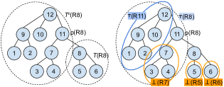
Figure 4: The given join tree consists of 12 relations. The node with number $i$ means $R_{i}$. The left figure circles the subtree rooted at $R_{8}$, $\mathcal{T}(R_{8})$, and the complementary subgraph of $\mathcal{T}(R_{8})$, $\mathcal{T}^{c}(R_{8})$. The right figure highlights that the multiplicity table of $R_{8}$, $T^{8}$, requires the join between the topjoin of $R_{8}$, ${\top}(R_{8})$ and the botjoins of all its children, $\{{\bot}(R_{5}),{\bot}(R_{6})\}$. The topjoin of $R_{8}$ can be iteratively computed from the join between the topjoin of the parent of $R_{8}$, i.e., ${\top}(R_{11})$, and the botjoins of the neighbors of $R_{8}$, i.e., $\{{\bot}(R_{7})\}$.

Algorithm. Algorithm 2 takes as input the join tree $\mathcal{T}$ of the acyclic query and database $\mathcal{D}$ . It first prepares botjoin and topjoin for each node with an iterative approach. To prepare botjoin $\bot(R_{i})$ (5), we start from the leaf nodes. The botjoin of a leaf node $R_{i}$ is simply a group by on the common attributes between $R_{i}$ and its parent node $p(R_{i})$ on $R_{i}$. Next, we compute ${\bot}$ for other nodes in a post-order traversal of the tree with this iterative formula:

$$\bot(R_{i})={\mathbf{\gamma}}_{\mathbb{A}_{i}\cap\mathbb{A}_{p(R_{i})}}(\widetilde{\mathbf{\bowtie}}(R_{i},\{\bot(R_{j})\mid R_{j}\in C(R_{i})\}))$$ (7)

For each ${\bot}(R_{i})$, the join starts with $R_{i}$ and follows by the children of $R_{i}$ one by one.

Example 5.2.

In Figure 4, we first compute the botjoins for all the leaf nodes including $\bot{(R_{1}})$, $\bot{(R_{2}})$, $\bot{(R_{3}})$, $\bot{(R_{4}})$,$\bot{(R_{5}})$, $\bot{(R_{6}})$, $\bot{(R_{10}})$. Next, if all the children of a node has a computed botjoin, then we can compute the botjoin of this node, e.g. ${\bot}(R_{8})={\mathbf{\gamma}}_{\mathbb{A}_{R_{8}}\cap\mathbb{A}_{R_{11}}}\left(\widetilde{\bowtie}\left(\widetilde{\bowtie}(R_{8},\bot{(R_{5})}),\bot{(R_{6})}\right)\right)$, where $R_{5}$ and $R_{6}$ are the children of $R_{8}$, and $R_{11}$ is the parent of $R_{8}$.

To prepare topjoin $\top(R_{i})$, we start with the children of the root node. The topjoin of each child $R_{i}$ of the root is the join between the root and the botjoins of all its neighbors followed by a group by on the common attributes between $R_{i}$ and the root. Next, we compute topjoin ${\top}$ for other nodes in a pre-order traversal of the tree with this iterative formula:

$$\top(R_{i})={\mathbf{\gamma}}_{\mathbb{A}_{i}\cap\mathbb{A}_{p(R_{i})}}(\widetilde{\mathbf{\bowtie}}(p(R_{i}),\top(p(R_{i})),\{\bot(R_{j})\mid R_{j}\in N(R_{i})\}))$$ (8)

For each $\top(R_{i})$, the join starts with $p(R_{i})$ and $\top(p(R_{i}))$ and follows by the botjoin of the neighbors of $R_{i}$ one by one. For example, computing the topjoin of $R_{8}$ in Figure 4 requires the join of its parent $R_{11}$, the topjoin of its parent ${\top}(R_{11})$, and the botjoins of all its neighbors, here $\{{\bot}(R_{7})\}$.

After preparing all the topjoins and botjoins, we combine these results to obtain the multiplicity tables $T^{i}$ for $i=1,\ldots,m$ based on Eqn. (6). For instance, to compute $T^{8}$ in Figure 4, we join the topjoin of $R_{8}$ and the botjoins of all its children, $\{\bot(R_{5}),\bot(R_{6})\}$. This does not require the topjoins of the root node or the botjoins of the leaf nodes. We iterate all the multiplicity tables $T_{i}$ and find the tuple with maximum ${\tt cnt}$. This tuple is returned as the most sensitive tuple with its ${\tt cnt}$ as the local sensitivity of this query on the given database instance.

The runtime of the algorithm depends on the max degree of the tree, which is the maximum children size + 1 (for a non-root node including the parent) of any node in the tree.

Algorithm 2 Compute Local Sensitivity of an acyclic CQ and the corresponding Most Sensitive Tuple

1:Acyclic CQ $Q_{{\tt acy}}(\mathbb{A}_{\mathcal{D}})$ as a join tree $\mathcal{T}$, the database ${\mathcal{D}}$

2:$LS(Q_{{\tt acy}},{\mathcal{D}})$, and the most sensitive tuple $t^{*}$

3:procedure LSAcyclicJoin

4:   I) Compute ${\bot}(R_{i})$ in post-order (leaf to root)

$$\begin{cases}{\mathbf{\gamma}}_{\mathbb{A}_{i}\cap\mathbb{A}_{p(R_{i})}}(R_{i}),&\text{if $R_{i}$ is leaf}\\ {\mathbf{\gamma}}_{\mathbb{A}_{i}}\widetilde{\bowtie}(R_{i},\{{\bot}(R_{j})\mid R_{j}\in C(R_{i})\}),&\text{if $R_{i}$ is root}\\ {\mathbf{\gamma}}_{\mathbb{A}_{i}\cap\mathbb{A}_{p(R_{i})}}\widetilde{\bowtie}(R_{i},\{{\bot}(R_{j})\mid R_{j}\in C(R_{i})\}),&\text{o.w.}\end{cases}$$

5:   II) Compute ${\top}(R_{i})$ in pre-oder (root to leaf)

$$\begin{cases}\emptyset,&\text{if $R_{i}$ is root}\\ {\mathbf{\gamma}}_{\mathbb{A}_{i}\cap\mathbb{A}_{p(R_{i})}}\widetilde{\bowtie}(p(R_{i}),\{{\bot}(R_{j})\mid R_{j}\in N(R_{i})\}),&\text{if $p(R_{i})$ is root}\\ {\mathbf{\gamma}}_{\mathbb{A}_{i}\cap\mathbb{A}_{p(R_{i})}}\widetilde{\bowtie}(p(R_{i}),{\top}(p(R_{i})),\{{\bot}(R_{j})\mid R_{j}\in N(R_{i})\}),&\hskip 3.0pt\text{o.w.}\end{cases}$$

6:   III) Prepare multiplicity tables $T^{i}$ of nodes for $i=1,\dots,m$

$$\begin{cases}{\mathbf{\gamma}}_{\mathbb{A}_{i}}({\top}{(R_{i}})),&\text{if $R_{i}$ is leaf}\\ {\mathbf{\gamma}}_{\mathbb{A}_{i}}\widetilde{\bowtie}(\{{\bot}(R_{j})\mid R_{j}\in C(R_{i})\}),&\text{if $R_{i}$ is root}\\ {\mathbf{\gamma}}_{\mathbb{A}_{i}}\widetilde{\bowtie}({\top}{(R_{i})},\{{\bot}(R_{j})\mid R_{j}\in C(R_{i})\}),&\text{o.w.}\end{cases}$$

7:IV) Select the most sensitive tuple

8:   $t^{*}=\operatorname*{arg\,max}_{t:t\in T^{i},i=1,\ldots,m}t.{\tt cnt}$ and $LS=t^{*}.{\tt cnt}$

9:   return $LS,t^{*}$

10:end procedure

Theorem 5.1.

Algorithm 2 computes the local sensitivity of an acyclic CQ and also finds the corresponding most sensitive tuple. Given $m$ tables with $k$ attributes in total, $n$ tuples in the database instance, and a join tree of the query with max degree $d$, the time complexity is $O(m~{}d~{}n^{d}~{}\log n)$.

Proof.

(sketch) If two nodes $R_{i}$ and $R_{j}$ share a common attribute $A$, then all the nodes on the path between $R_{i}$ and $R_{j}$ in the join tree also contain $A$. Hence, the iterative equations (7) and (8) correctly compute the botjoin (5) and topjoin (4) by tracking multiplicities through common attributes.

Now we analyze the running time of the algorithm. Notice that all joins in any topjoin equation (8) and botjoin equation (7) have at least one common join attribute, according to the definition of join tree and the fact that the projection of ${\top}(R_{i})$ and ${\bot}(R_{i})$ is always the subset of $\mathbb{A}_{i}$ and $\mathbb{A}_{p(R_{i})}$. For botjoin (7), we join relations with $R_{i}$ one at a time using sort-merge-join and then do groupby count. The size of each join is always $\leq n_{i}$ since each tuple $R_{i}$ can join at most one tuple from any botjoin of its children. In total, it takes $O(d_{i}n_{i}\log n_{i})$ for each botjoin and $O(mn\log n)$ for all botjoins since the summation of $d_{i}$ is m and $n_{i}\leq n$.

Next we discuss the running time for step III) in Algorithm 2. Unlike the computation for topjoins and botjoins, this step requires joining the botjoins of all the children of a node with the topjoin of that node $R_{i}$, and all these partial joins may not share any attributes in general (although all the join attributes are still subsets of $\mathbb{A}_{i}$). Hence, for arbitrary acyclic joins, there can be at most $d-1$ joins in this step for each $R_{i}$ where $d$ is the max degree in $\mathcal{T}$, which can be computed in $O(n^{d}\log n^{d})=O(dn^{d}\log n)$ time even by the brute force approach. The total time to compute the multiplicity tables $T^{i}$ for $m$ relations is $O(mdn^{d}\log n)$. Hence, the total time complexity is $O(mdn^{d}\log n)$. ∎

Similar to the discussion in Section 4.2, the computation of botjoins ${\bot}(R_{i})$ and topjoins $\top(R_{i})$ in Algorithm 2 is inspired by Yannakakis’s algorithm [46], which can track counts of intermediate tuples from the leaves to the root in a bottom-up pass, whereas in the second top-down pass, we need to traverse the join tree to compute the topjoins ${\top}({R_{i}})$. As explained earlier for path queries, Algorithm 2 computes changes in the join size for all possible tuple deletions and additions, and naively repeating [46] to evaluate query on all possible databases formed by adding or removing a tuple does not give the desired complexity. In fact, [46] works in near-linear time in the input size $n$ to output the output join size for any acyclic join query (and has polynomial combined complexity), whereas the sensitivity problem is NP-hard in combined complexity even for acyclic queries as stated in Theorem 3.2.

Given the NP-hardness result in Theorem 3.2, we next show an example acyclic query that may take $\omega(mn)$ time for the $T^{i}$ step. Suppose we have an acyclic query as $Q(A,B,C):-R_{1}(A,B,C),R_{2}(A,B),R_{3}(B,C),R_{4}(C,A)$ and we want to compute the multiplicity table $T^{1}$ for $R_{1}$. Given botjoins of $R_{2}(A,B)$, $R_{3}(B,C)$ and $R_{4}(C,A)$, we have a cyclic join among them, and in worst the join size is $O(n^{3/2})$ according to the AGM bound [9]. In general, if we replace the children with more complex queries, and if the number of relations (or the degree) is larger, the time to compute this join may be larger. Note that some of the complexity of this problem comes from the bag semantics considered in our model (that is also relevant for applications of sensitivity related to differential privacy), as for set semantics, changes in the join size can be computed more efficiently when a tuple is added or removed from a table. However, for bag semantics, adding any tuple, say to $R_{1}$, may increase the sensitivity significantly for $Q$ (product of the multiplicities of the edges forming the triangle), which adds to the complexity.

5.3 Doubly Acyclic Join Queries

For an acyclic query, if there exists a join tree $\mathcal{T}$ constructed from the GYO decomposition such that for each node $R_{i}$ in $\mathcal{T}$, the join between its parent $p(R_{i})$ and its children $C(R_{i})$ is also acyclic, then we say this query is a doubly acyclic join query. Given this property, the computation of the multiplicity table $T_{i}$ for $R_{i}$ involves an acyclic join between the topjoin and botjoins and hence has a time complexity $O(d_{i}n_{i}\log n_{i})$, where $d_{i}$ is the node degree of $R_{i}$ in $\mathcal{T}$. Since the sum of all node degrees is $m$ and $n_{i}\leq n$, the total time complexity to compute $T^{i}$ for all nodes is $O(mn\log n)$. When $d_{i}$ is a constant, such as at most 2, the complexity is written as $O(n\log n)$, which also matches the total runtime of Algorithm 2 including the computation of topjoins and botjoins.

Notice that a path join query is a special case of doubly acyclic join query, because for each $R_{i}$, ${\top}(R_{i})$ and ${\bot}(R_{i+1})$ (assuming $R_{i+1}$ is the child of $R_{i}$ in $\mathcal{T}$) share no attributes. and therefore is an acyclic join. The time complexity of path join queries in Algorithm 1 also matches the time complexity of doubly acyclic join queries.

5.4 Extensions

In this section we briefly discuss how to extend our framework relaxing the assumptions listed at the beginning of Section 5, and we defer the details in a full version.

Selections: We can easily extend Algorithm 2 to handle queries with arbitrary selection conditions (that can be applied to each tuple individually in any relation) in the body of the query by assigning 0 sensitivity to the tuples fail the selection condition.

Disconnected join trees: If the hypergraph of a query is not connected, Algorithm 2 can be applied to each join tree and merge them back to update each tuple sensitivity.

General joins: For a non-acyclic join query, if there exists a generalized hypertree decompositions[5] such that we can find a join plan from this tree by assigning each relation to one node, Algorithm 2 can be extended by computing the multiplicity table as including other relations within the same node, and the time complexity is parameterized by the max number $p$ of relations within a node as $O(mpdn^{pd}\log n)$. This is implemented in our experiments; q3 from TPC-H queries, and $q_{\triangle}$, $q_{\square}$ from Facebook queries are all non-acyclic queries and their generalized hypertree decompositions are shown in Figure 5.

Efficient approximations: We can extend our algorithm to tradeoff accuracy in the sensitivity for better runtime. As our experiment will show, the multiplicity tables that topjoins and botjoins compute can grow quadratically or faster in the input size depending on the query. To make the computation scalable, we can maintain the top $k$ frequent values instead of all the frequencies in the top and botjoins. We can set the frequencies of the rest of the active values in the top and botjoins to the kth largest frequency. This approach gives an upper bound of tuple sensitivity but can speed up runtime.

Self Joins: Acyclic join queries with self-joins can not be captured by our algorithms, because we only allow a relation to appear once in the query. For each relation, we compute the joins for the rest of relations to summarize how tuples from this relation can affect the full join. A possible workaround is to join the repeated base relations as a single and combined relation, run our algorithm, and then link the effect of adding or removing a tuple from the base relation to the combined relation and the effect of adding or removing a tuple from the combined relation to the rest. However, it is challenging to find all possible insertions to the base relation that allows the combined relation to join all possible pairs of ”incoming” and ”outcoming” path. We defer this line of research to future work.

Other: For attributes that appear only once in the query body, we ignore them in Algorithm 2 but in the end we extrapolate a value for these attributes.

6 Use in Differential Privacy

In this section, we will show how to use our algorithm TSens (section 5.2) for computing sensitivity to develop accurate differentially private algorithms. Section 6.1 gives a brief overview of differential privacy (DP), and Section 6.2 discusses how the tuple sensitivity measures can be used to develop accurate DP algorithms.

6.1 Differential Privacy

Differential privacy (DP) [19] is considered the gold standard for private data analysis. An algorithm satisfies DP if its output is insensitive to adding or removing a tuple in the input database. Formally,

Definition 6.1 (Differential Privacy).

A mechanism $\mathcal{M}:I\rightarrow\Omega$ is $\epsilon$-differentially private if for any two neighbouring relational database instances ${\mathcal{D}},{\mathcal{D}}^{\prime}\in I$ and $\forall O\subseteq\Omega$:

$$\left|\ln(\Pr[\mathcal{M}({\mathcal{D}})\in O]/\Pr[\mathcal{M}({\mathcal{D}}^{\prime})\in O])\right|\leq\epsilon$$

When ${\mathcal{D}}$ is a single relation, all neighboring relations are of the form ${\mathcal{D}}^{\prime}={\mathcal{D}}-\{t\}$. When ${\mathcal{D}}$ is a multi-relational database with foreign key constraints, then a neighboring instance ${\mathcal{D}}^{\prime}$ is gotten by deleting one tuple $t$ in ${\mathcal{D}}$’s primary private relation and cascadingly deleting other tuples that depend on $t$ through foreign keys [30].

Differential privacy has been successfully used to publish summary statistics, synthetic data, machine learning models, and answer SQL queries [40, 45, 2, 42, 35, 26, 30] . It has also been adopted at government [4] and commercial organizations [22, 44, 12, 18, 10].

Laplace Mechanism is a fundamental building block of DP algorithms [20]. It answers a query $Q$ by adding noise drawn from a Laplace distribution scaled to the ratio of the global sensitivity of $Q$ and the privacy loss parameter $\epsilon$.

Definition 6.2 (Global Sensitivity).

Given a counting query $Q:I\rightarrow\mathcal{R}$, the global sensitivity $GS$ is defined as the max difference of query result from any two neighbouring relational database instances ${\mathcal{D}},{\mathcal{D}}^{\prime}\in I$ :

$$GS(Q)=\max_{({\mathcal{D}}^{\prime}-{\mathcal{D}})\cup({\mathcal{D}}-{\mathcal{D}}^{\prime})=\{t\}}\left|Q({\mathcal{D}})-Q({\mathcal{D}}^{\prime})\right|$$

Unlike the local sensitivity of a query which depends on the given database instance, the global sensitivity of a query finds the largest possible local sensitivity among all possible database instances. Consider the join query in Figure 1(b), Example 2.1 shows that it has a local sensitivity of 4 on the database instance shown in Figure 1(a). However, there exist other database instances with a much larger local sensitivity than 4. For example, if $R_{2}$ in Figure 1(a) has 1000 copies of $(a_{1},b_{1},d_{1})$ which results in 1000 copies of $(a_{1},b_{1},c_{1},d_{1},e_{1},f_{1})$ in the join output, removing $(a_{1},b_{1},c_{1})$ from $R_{1}$ can result in a change of 1000 in the output size. If there is no a priori bound on the number of tuples that share the same join key, the global sensitivity of the query will be unbounded.

Definition 6.3 (Laplace Mechanism).

Given a counting query $Q:I\rightarrow\mathcal{R}$, a database instance ${\mathcal{D}}\in I$ and a privacy parameter $\epsilon$, the following noisy query result satisfies $\epsilon$-DP: $Q({\mathcal{D}})+\eta$, where $\eta\sim exp(-\frac{|\eta|\cdot\epsilon}{GS(Q)})$.

The noise $\eta$ has a mean 0 and a variance of $2GS(Q)^{2}/\epsilon^{2}$ which increases with the global sensitivity of the query. Hence, this mechanism cannot be directly applied to query with unbounded global sensitivity. Prior work for general join queries either have high performance cost [29, 13, 17] or suffer from poor accuracy [26]. One effective and general purpose technique from prior work is truncation that executes the query $Q$ on a truncated version of the database $T({\mathcal{D}})$ [35, 30]. The truncation is done in such a way that $Q(T(\cdot))$ has a bounded global sensitivity. For a join, this might mean removing rows from the database such every join key has a bounded selectivity. We will next show a truncation based algorithm for answering SQL aggregation queries with joins based on the tuple sensitivities.

6.2 Truncation mechanism with TSens

The idea behind our algorithm is to (a) identify tuples in the database (i.e., in the primary private relation) that have a sensitivity greater than a sensitivity threshold, and (b) remove all tuples with sensitivity greater than the sensitivity threshold.

Definition 6.4 (TSens Truncation).

Given a query $Q$, a database ${\mathcal{D}}$ with primary private relations $\mathcal{PR}$, and a sensitivity threshold $i$, the truncation operator $T_{\textnormal{{TSens}}}$ transforms the database as:

$$T_{\textnormal{{TSens}}}(Q,{\mathcal{D}},i)=\left\{t\in{\mathcal{D}}\mid t\in\mathcal{PR}\Rightarrow\delta(t,Q,{\mathcal{D}})\leq i\right\}$$

The global sensitivity of $Q(T_{\textnormal{{TSens}}}(Q,\cdot,\tau))$ is $\tau$. If we add or remove a tuple with sensitivity more than $\tau$, the query result does not change as the new tuple will be truncated or has already been truncated. Since the largest possible tuple sensitivity is $\tau$ for any database, the global sensitivity is $\tau$. Hence, given a join query $Q$ with high global sensitivity, we can first apply $Q(T_{\textnormal{{TSens}}}(Q,\cdot,\tau))$ to the database and then apply Laplace mechanism with smaller noise (due to smaller global sensitivity) on the transformed database. However, the transformed database also introduces bias if too many tuples are truncated. Hence, we would like to find a truncation threshold that minimizes the expected sum of bias and noise.

Finding truncation threshold.  If setting $\tau$ to be the local sensitivity of the query $Q$, then $Q({\mathcal{D}})=Q(T_{\textnormal{{TSens}}}(Q,\cdot,\tau))$, i.e., no bias is introduced. However, using local sensitivity directly violates DP. Moreover, the global sensitivity of querying the local sensitivity of a join query is unbounded, we cannot use Laplace mechanism to release a noisy local sensitivity. Instead, line in PrivSQL [30], we apply the sparse vector technique (SVT) [34] to find the optimal truncation threshold that is close to the local sensitivity.

For a query $Q$ and a database ${\mathcal{D}}$, let $\ell$ be an upper bound on the local sensitivity. We first release a noisy version of $Q(T_{\textnormal{{TSens}}}(Q,{\mathcal{D}},l))$ as $\hat{Q}$ using the Laplace mechanism with global sensitivity as $\ell$. Next, we run the SVT method that checks whether $q_{i}>0$ for $i=1,\ldots,\ell-1$, where

$$q_{i}=\frac{Q(T_{\textnormal{{TSens}}}(Q,{\mathcal{D}},i))-\hat{Q}}{i}$$

Since the global sensitivity of $Q(T_{\textnormal{{TSens}}}(Q,{\mathcal{D}},i))$ is $i$, the global sensitivity of each $q_{i}$ is a constant 1. SVT stops the first time (noisy) $q_{i}$ is above the (noisy) threshold 0 and reports $i$. We take this $i$ as the truncation threshold $\tau$, and answer the query $Q$ using $Q(T_{\textnormal{{TSens}}}(Q,{\mathcal{D}},i))$. A part of the privacy budget $\epsilon_{tsens}$ is used to release $\hat{Q}$ and run SVT for finding the truncation threshold $\tau$. The rest $\epsilon-\epsilon_{tsens}$ is used to answer the query.

Theorem 6.1.

The algorithm that finds the truncation threshold satisfies $\epsilon_{tsens}$-DP and releasing a noisy answer as $Q(T_{\textnormal{{TSens}}}(Q,{\mathcal{D}},\tau))+Lap(\frac{\tau}{\epsilon-\epsilon_{tsens}})$ satisfies $(\epsilon-\epsilon_{tsens})$-DP. Together the mechanism satisfies $\epsilon$-DP.

Discussion.  Our solution is inspired by Wilson et al [44], but they handle can only handle a single join (and not self joins), while we can handle a wider sub-class of full conjunctive queries without self joins. Moreover, Wilson et al set the sensitivity threshold manually, while we automatically identify the threshold given an estimated upper bound.

Our algorithm truncates primary private tables while in PrivSQL [30], truncation happens at non-primary private tables. PrivSQL truncates tuples with high frequencies, but it doesn’t mean that they join with the tuple of the highest tuple sensitivity. In contrary, truncation by tuple sensitivity is a finer truncation strategy which reduces global sensitivity and bias at the same time.

Our algorithm for finding the most sensitive tuples can be easily extended for TSens by storing the multiplicity table for the primary private table. Our truncation algorithm takes in estimated upper bound of tuple sensitivity $\ell$. Our algorithm will still ensure DP regardless of the value for $\ell$, but the value of $\ell$ can affect the accuracy. We illustrate the impact of $\ell$ on the accuracy in the evaluation.

7 Experiments

We evaluate the efficiency and accuracy of TSens. Experiments are designed to answer following questions:

• How tight is the local sensitivity computed by TSens compared to other algorithms like elastic sensitivity [27]?

• How does TSens’ runtime compared to that of (a) the elastic sensitivity algorithm and (b) query evaluation?

• Does the truncation with TSens mechanism result in more accurate differentially private query answering than prior work like PrivSQL [30]?

We use synthetic datasets from TPC-H benchmark [1] and real world datasets of Facebook ego-networks from SNAP [32] and designed seven full conjunctive queries with different query complexities to evaluate the performance of TSens. These queries are also used to evaluate the performance of DP mechanism supported by TSens. The results are compared with the sensitivity engine Elastic from ‘Flex’ [27] and with the differentially private SQL answering engine PrivSQL from ‘PrivateSQL’ [30]. We name our sensitivity algorithm as TSens and its DP application as TSensDP.

A summary of our key findings:

• TSens achieves at most 2,200,000 times smaller local sensitivity compared to Elastic for a simple cyclic query for a database with 866,602 tuples.

• TSens has on average 80% - 320% overhead compared to query evaluation for different queries. It is 2 - 60 times slower than Elastic, but returns a local sensitivity value that is 6 - 60,000 times smaller on average.

• PrivSQL has more than 99% relative error (almost worse than just returning 0 as the answer) for four of the seven queries. TSensDP answers 8 queries with $\leq 8\%$ relative error and the last query with $\leq 20\%$ relative error.

7.1 Setup

(a) TPC-H queries

(b) Facebook queries

Figure 5: The join plan for each query.

Dataset. We evaluate our algorithms on synthetic TPC-H datasets [39] and real world Facebook dataset [32].

TPC-H. We consider synthetic datasets generated from TPC-H benchmark [39] with the following schema:
Attributes: RegionKey(RK), NationKey(NK), CustKey(CK), OrderKey(OK), SuppKey(SK), PartKey(PK)
Relations: Region(R:RK), Nation(N:RK,NK), Customer(C:NK,CK), Orders(O:CK,OK), Supplier(S:NK,SK), Part(P:PK), Partsupp(PS:SK,PK), Lineitem(L:OK,SK,PK).

We evaluate the scalability of our algorithm on TPC-H datasets at different scales $\{0.0001,0.001,0.01,0.1,1,2,10\}$. At scale 1, the sizes of for these relations are 5, 25, 1e4, 1.5e5, 2e5, 8e5, 1.5e6, 6e6 respectively. The same schema and datasets were used to evaluate prior work on differentially private SQL query answering [27, 30].

Facebook. We use the Facebook ego-networks from SNAP (Stanford Network Analysis Project) [32]. An ego-network of a user is a set of “social cirles” formed by this user’s friends [33]. This dataset consists 10 ego-networks, 4233 circles, 4039 nodes and 88234 edges. We choose the ego-network of user 348 who has 567 circles, 225 nodes and 6384 edges, create edge tables $E_{i}(x,y)$ for each circle $i$ such that both users of each edge is from the circle $i$ and sort them by table size in descending order. We further create tables $R_{1}(x,y)$, $R_{2}(x,y)$, $R_{3}(x,y)$, $R_{4}(x,y)$ and insert $E_{j}$ into $R_{i}$ if the rank of $E_{j}$ mod 4 = i. We also create a 3-column table $R_{\triangle}(x,y,z):-R_{4}(x,y),R_{4}(y,z),R_{4}(z,x)$ as a triangle table. All edges are bi-directed.

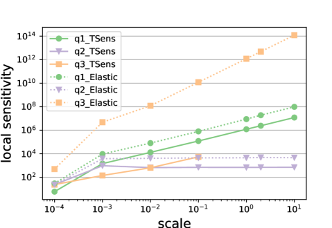
(a) Local sensitivity reported by TSens and Elastic for queries q1, q2 and q3 on datasets of differing scales

(b) Most sensitive tuples and their tuple sensitivities for each relation of q3 when scale = 0.01.

Figure 6: Local sensitivity reported by TSens versus Elastic for TPC-H queries

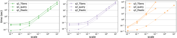
Figure 7: The trend of time usage in terms of various scales for queries q1, q2 and q3 and algorithms TSens and Elastic for TPC-H queries. The base line ‘query’ shows the query evaluation time.

Queries. We consider 3 TPC-H queries and show their query plan in Figure 5(a) which include a path join query q1, an acyclic join query q2, and a cyclic join query q3. The third query q3 is a cyclic join query that builds a universal table with an extra constraint that the supplier and customer should be from the same nation. We also consider 4 Facebook queries as shown in Figure 5(b) including a triangle query $q_{\triangle}(A,B,C)$, a path join query $q_{w}(A,B,C,D,E)$, a 4-cycle query $q_{\square}(A,B,C,D)$, and a star join query $q_{\Yup}(A,B,C)$. We also show the generalized hypertree decomposition for all non-acyclic queries in the same figure.

We use a machine with 2 processors, 512G SSD and 16G memory to run experiments. Each query is repeated 10 times.

7.2 Local Sensitivity

Baseline. We compare the accuracy and runtime of our TSens algorithm with prior technique Elastic [27] for finding the local sensitivity of a given query. As the original Elastic algorithm requires the maximum frequency of the join attributes to derive the upper bound of the local sensitivity, we first let Elastic pre-process the database to obtain the max frequency for its sensitivity analysis. We also extend Elastic algorithm to support cross-product by assigning the max frequency of empty attributes as the size of the table and to take the join plan as input so that the join order in the experiment is the same. We define the join order as a post-traversal of the join plan.

We also compare the algorithm runtime to the query evaluation time. We apply Yannakakis algorithm to compute the size of query output. For queries that are not acyclic, we first compute the join for each node in the generalized hypertree, and then apply Yannakakis algorithm. The time of running Elastic is also reported. We run each algorithm 10 times to report the average time.

Result and Analysis. Figure 6(a) shows the local sensitivity trend in aspect to the scale for TPC-H. Notice that after scale 0.001, TSens has on average 7x smaller and 6x smaller of the local sensitivity for q1 and q2 than Elastic has. Moreover, for q3, TSens achieves 2,200,000x smaller value for the local sensitivity than Elastic does when scale equals to 0.1. We didn’t run q3 for scale larger than 0.1 due to the memory limit issue. The multiplicity tables for this cyclic query grows nearly quadratically with the input table size. Our future work will extend our algorithm to maintain the top $k$ frequent values instead of all the frequencies which can reduce the intermediate size and further speed up runtime (Section 5.4).

Figure 6(b) shows the most sensitive tuple found by TSens for each relation for q3 at scale = 0.01. Unlike TSens, Elastic can only obtain a local sensitivity upper bound, but cannot find the most sensitive tuple. Hence, we report the most sensitive tuple for each relation while also reports its elastic sensitivity by setting this relation as the only sensitive table for Elastic. Each tuple sensitivity found by TSens is below 1,000 while the least elastic sensitivity reported by Elastic is beyond 10,000. We skip finding the most sensitive tuple in LINEITEM since it has the superkey in the query head and thus the tuple sensitivity is at most 1.

Figure 7 shows the time cost for both TSens and Elastic for different queries and scales for TPC-H. The second line $q_{i}\_query$ is the query evaluation time. Notice that we skip computing the multiplicity table of Lineitem in q3 since the tuple sensitivity is at most 1 due to FK-PK joins. For q1 and q2, both TSens and Elastic shows a tight relation to the time of query evaluation, which takes on average 1.8x and 0.9x of the query evaluation time after scale 0.001. For q3, although Elastic is much faster, TSens only takes on average 4.2x of the query evaluation time to find on average 60,000x smaller local sensitivity before scale 1.

We also report the accuracy and the runtime of TSens and Elastic for Facebook queries in Table 1. The sensitivity bound improvement ranges from $\times 3$ to $\times 80k$. Although TSens spends $\times 25$ to $\times 60$ more time than Elastic, its runtime is comparable to query evaluation time. The local sensitivity can also be computed by repeating query evaluation over databases which are formed by removing a tuple from active domain or inserting a tuple from representative domain one at a time (using a variation of [46] as discussed in Sections 4.1 and 5.2). However, the size of the active domain and representative domain is above 10k. This approach will take $\times 10k+$ time than TSens.

	Local Sensitivity		Time (seconds)
	TSens	Elastic	TSens	Elastic	Evaluation
$q_{\triangle}$	87	7524	0.405	0.007	0.431
$q_{w}$	178923	511632	0.237	0.010	0.182
$q_{\square}$	2014	511632	0.618	0.009	0.465
$q_{\Yup}$	34	2723688	0.604	0.012	0.175

Table 1: Local sensitivity and runtime of 4 query types for TSens and Elastic for Facebook queries. It also reports the query evaluation time for counting the output size. Gray cells have tighter local sensitivities.

Qu- ery	${|Q(D)|}$	Algorithm	Error	Bias	Global Sens.	Time
q1	60175	TSensDP	3.56%	3.44%	119	0.693
		PrivateSQL	1.34%	1.02%	220	0.292
q2	60175	TSensDP	7.71%	7.62%	640	0.554
		PrivateSQL	99.03%	100.00%	774	0.231
q3	2333	TSensDP	2.84%	0.00%	14	23.063
		PrivateSQL	1293%	2.14%	12375k	0.546
$q_{\triangle}$	30699	TSensDP	1.50%	1.47%	49	0.562
		PrivateSQL	19.12%	0.00%	6732	0.230
$q_{w}$	17555419	TSensDP	5.59%	5.69%	17440	0.843
		PrivateSQL	2.25%	0.00%	289476	10.340
$q_{\square}$	142903	TSensDP	2.00%	1.77%	167	0.792
		PrivateSQL	100%	0.00%	289476	2.232
$q_{\Yup}$	786	TSensDP	19.02%	16.16%	13	0.670
		PrivateSQL	30K%	0.00%	2437K	0.290

Table 2: Application to DP: Comparison between TSensDP and PrivSQL for TPC-H and Facebook queries. Time is in seconds. Gray cells achieve lower errors.

7.3 Differential Privacy

Baseline. PrivSQL is a differentially private SQL answering engine and it introduces the concept of policy that given primary private relations, the sensitivity of other related relations should be updated to be non-zero according to the database key constraints. For TPC-H datasets, we consider CUSTOMER is the primary private relation for q1 and q3, and SUPPLIER is the primary private relation for q2, so the sensitivity of ORDERS is affected by CUSTOMER and the sensitivity of PARTSUPP is affected by SUPPLIER. The sensitivity of LINEITEM is affected by either of them. For Facebook dataset, we consider $R_{2}$ is the primary private relation.

PrivSQL uses the maximum frequency as the truncation threshold, which is different from using tuple sensitivity to truncate the database. Any tuple whose frequency is beyond the max frequency will be dropped from the database. PrivSQL runs SVT to learn the truncation threshold for each relation; however, the noise scale of SVT depends on the sensitivity of the relation while it is constantly 1 in TSensDP.

Although the privacy budget allocation strategy affects the performance of DP algorithm, we skip exploring this effect and assume PrivSQL and TSensDP divide the privacy budget into two halves, one for the threshold learning and the other for reporting the query result after truncation. We disable the synopsis generation phase of PrivSQL and just use Laplace mechanism to answer the SQL query directly.

Result and Analysis. Table 2 shows the statistics of releasing differential private query results by TSensDP or PrivSQL for TPC-H and Facebook datasets. Output below 0 is truncated to 0. We report the median of global sensitivity, the median of relative absolute bias, the median of relative absolute error and the average time for each query over 20 runs. We assume the table size is given. For TPC-H, we assume the maximum tuple sensitivity of q1 is 100, of q2 is 500 and of q3 is 10. TSensDP has $\leq 4$% error for $q_{1}$ and $q_{3}$, and $\leq 8$% error for $q_{2}$. In contrast, PrivSQL has more than $99$% error on $q_{2}$ and $q_{3}$. This means that the error in PrivSQL answers for these queries is worse than returning 0 as the answer without looking at the data. The reasons for the poor error are different. In $q_{2}$ PrivSQL truncates too much of the data, while in $q_{3}$ it estimate a very loose bound on sensitivity.

For Facebook dataset, we assume the maximum tuple sensitivity of $q_{\triangle}$ is 70, of $q_{w}$ is 25k, of $q_{\square}$ is 200 and of $q_{\Yup}$ is 15. TSensDP achieves $<6\%$ error for $q_{\triangle}$, $q_{w}$, $q_{\square}$, while PrivSQL get $>100\%$ error for $q_{\square}$ and $q_{\Yup}$. Since there is no FK-PK join for Facebook queries, we have only one primary private table, which means no table truncation and thus has 0 bias in PrivSQL. However, PrivSQL has $\times 10$ to $\times 180k$ larger global sensitivity than TSensDP, which dominates the error.

Parameter Analysis. To find how the upper bound parameter for tuple sensitivity $\ell$ affects the performance, we vary $\ell$ through 1, 10, 30, 50, 100, 1000 and repeat TSensDP 20 times for the star query $q_{\Yup}(A,B,C)$ whose true local sensitivity is 13 when $R_{2}$ is the primary private relation for DP. For each bound, the median global sensitivity, which is also the tuple sensitivity threshold learned from the SVT routine, is [11, 13, 9, 4, 48, 160], the median bias error is [3%, 1%, 13%, 55%, 0%, 0%], and the median relative error is [5%, 4%, 17%, 56%, 32%, 98%]. The optimal $\ell$ in this case is 10, with the corresponding error as 4%, while the worst error is 98% when $\ell=1000$.

Notice that as $\ell$ increases, the noise added to $\hat{Q}$ in the SVT routine gets larger. This causes the learned tuple sensitivity threshold to deviate more from the local sensitivity, which is considered the optimal threshold by the rule of thumb. When $\ell$ is too small, the learned tuple sensitivity threshold could also be small, which increases the bias.

8 Related Work

Sensitivity analysis for SQL queries is important to the design of differentially private algorithms. The focus of existing work [38, 31, 8, 21, 30, 35] is to compute the global sensitivities of SQL queries or their upper bounds. The earliest work by McSherry along this line [35] applies static analysis on a given relational algebra and then combines the sensitivities of the operators in the relational algebra to obtain the maximum possible change to the query output for all possible database instances. This analysis is independent of the database instance, so the result can be much larger than the local sensitivity. In particular, for join operator, the global sensitivity can be unbounded. The analysis either considers a restricted form of join [35, 21] or constrained database instances [38, 31, 8]. For general join queries on unconstrained databases, Lipschitz extension [29, 13, 17, 30] is usually applied to transform the original query $Q$ that has an unbounded sensitivity into a different query $Q^{\prime}$ that (a) has abounded global sensitivity and (b) has a similar answer as $Q$. In particular, the transformed query in PrivateSQL [30] require to truncates the sensitive tuples. Hence, our work offers efficient ways to identify the most sensitive tuples to complement PrivateSQL to achieve differential privacy.

Smooth sensitivity [37, 26] is another important sensitivity notion for achieving differential privacy. This sensitivity is a smooth upper bound of the local sensitivity of databases at a distance from the given database instance. This requires the computation of local sensitivity of exponentially number of database instances. For SQL queries, elastic sensitivity [26] provides efficient static analysis rule to estimate the upper bound of local sensitivity, but this bound can be still very loose. For example, even if the local sensitivity for a query with selection operator is small, the elastic sensitivity algorithm will output the same value as for a query without the selection operators. In addition, the computation of elastic sensitivity requires additional constraint cardinality information of the given database instance.

Smooth sensitivity [37, 47] or Lipschitz extension [17, 29, 13] have been mainly applied to release graph statistics. However, these algorithms either require customized analysis for each new query [47] or suffer from high performance cost [37, 17, 29, 13]. We will extend our study to graph queries (involving self-joins) in the future.

Sensitivity analysis has also been studied for non-SQL functions [24, 41, 15], with a focus on global sensitivity. Related topics also include sensitivity analysis for probabilistic queries [28] and finding responsibility of tuples [36], where the goal is different from ours. Prior work on provenance for queries and deletion propagation (e.g., [7, 14]) provide analysis for a rich set of queries and explanations for query results, but the analysis is mainly for removing a tuple in the database (downward tuple sensitivity). Our work also considers upward tuple sensitivity which involves adding new tuples from the domain. Our future study will consider general aggregates and functions.

9 Conclusions

We studied the local sensitivity problem for counting queries with joins – an important task for many applications like differentially private query answering and query explanations. We showed that the problem is NP-hard in combined query and data complexity even for full conjunctive queries that have an acyclic structure – queries for which the combined complexity of query answering is PTIME. We develop algorithms for full acyclic join queries using join trees, that run in linear in the number of relations and near linear in the number of tuples for interesting sub-classes of acyclic queries including path queries and “doubly acyclic queries”, and in PTIME in combined complexity when the maximum degree in the join tree is bounded. Our algorithms can be extended to handle related queries that include selection predicates as well as non-acyclic queries with a certain property on generalized hypertree decompositions. The local sensitivity output by our algorithms is shown to be orders of magnitude tighter than prior work. Our algorithm can also be used to construct differentially private query answering methods that are more accurate than the state of the art. Extending the framework to handle general non-acyclic queries involving self-joins, projections, negations, and other aggregate functions would be an interesting direction of future work.

Appendix A Theorem and Proofs

A.1 Proof for Theorem 3.1

Proof.

(Algorithm) The algorithm works as follows. First, compute the maximum downward tuple sensitivity $\delta^{-*}=\max_{t\in Q({\mathcal{D}})}\delta^{-}(t,Q,{\mathcal{D}})$ (see Definition 2.1), and note the tuple giving the max value. Next, compute the maximum upward tuple sensitivity as $\delta^{+*}$ = $\max_{i\in\{1,\cdots,m\}}\max_{t\in\Sigma_{repr}^{\mathbb{A}_{i}}}\delta^{+*}(t,Q,{\mathcal{D}})$, again noting the tuple giving the maximum value. Return $\delta^{*}=\max(\delta^{+*},\delta^{-*})$ along with the tuple that led to this highest value.

(Correctness) We omit the proof that this algorithm correctly computes the local sensitivity due to space constraints.

(Polynomial data complexity) Finally we argue that the algorithm runs in time polynomial in $n=|D|$. Note that the active domain of any single attribute $A\in\mathbb{A}_{D}$ in any relation $R_{i}$ can be computed in time polynomial in $n$ (in $O(n\log n)$ time if we use sorting to remove duplicates), and $|\Sigma_{act}^{A,i}|\leq n$. Since each relation $R_{i}$ has at most $k$ attributes, $|\Sigma_{repr}^{\mathbb{A}_{i}}|\leq n^{k}$. Hence the above algorithm iterates over polynomial number of choices for $t$, for each $t$ it evaluates the query $Q(D\cup\{t\})$ or $Q(D-\{t\})$, which can be done in polynomial time in $n$. Hence the total time of the above algorithm is also polynomial in $n$. ∎

A.2 Proof for Theorem 3.2

Proof.

We give a reduction from the 3SAT problem. Consider any instance of 3SAT $\phi$ with $s$ clauses ($C_{1},\ldots,C_{s}$) and $\ell$ variables ($v_{1},\ldots,v_{\ell}$), where each clause is disjunction three literals (a variable or its negation), and the goal is to check if the formula $\phi=C_{1}\wedge\cdots\wedge C_{s}$ is satisfiable. We create an instance of the sensitivity problem $LS(Q,{\mathcal{D}})$ with $s+1$ relations and $\ell$ attributes in total. For each clause $C_{i}$ that involves variables $v_{i_{1}},v_{i_{2}},v_{i_{3}}$, we add a table $R_{i}$ with three Boolean attributes $A_{i_{1}},A_{i_{2}},A_{i_{3}}$, and insert all possible triples of Boolean values that satisfy the clause $C_{i}$ into $R_{i}$ in ${\mathcal{D}}$. For example, if $C_{i}$ is $v_{2}\lor\bar{v}_{5}\lor\bar{v}_{7}$, then $R_{i}(A_{2},A_{5},A_{7})$ contains seven Boolean triples $(0,0,0),(0,0,1),\ldots,(1,1,1)$ except $(0,1,1)$. In addition, we create an empty relation $R_{0}(A_{1},\ldots,A_{\ell})$, which does not contain any tuple in ${\mathcal{D}}$. The query is:

$$Q(A_{1},\ldots,A_{\ell})=R_{0}(A_{1},\cdots,A_{\ell})\wedge\underset{i=1,\ldots,m}{\bigwedge}R_{i}(A_{i_{1}},A_{i_{2}},A_{i_{3}})$$

Note that $Q$ is acyclic, as all of $R_{1},\cdots,R_{s}$ correspond to ears (see Section 2.2). Further, the reduction is in polynomial time in the number of variables and clauses in $\phi$. Next we argue that $\phi$ is satisfiable if and only if $LS(Q,{\mathcal{D}})>0$.

(only if) Suppose $\phi$ is satisfiable, and $\mathbf{v}=(v_{1}=b_{1},\cdots,v_{\ell}=b_{\ell})$ is a satisfying assignment. Then the join of $R_{1}\Join\cdots\Join R_{s}$ is not empty and $\mathbf{v}$ belongs to their join result. However, $Q({\mathcal{D}})=\emptyset$ as $R_{0}=\emptyset$ in ${\mathcal{D}}$. Now, if we add a tuple corresponding to $\mathbf{v}$ to $R_{0}$, then $Q({\mathcal{D}}\cup\{\mathbf{v}\})$ is no longer empty (at least contains $\mathbf{v}$), and therefore $LS(Q,{\mathcal{D}})>0$.

(if) Suppose $LS(Q,{\mathcal{D}})>0$. Hence there exists at least one tuple $t$ such that if it is added to one of the relations $R_{0},R_{1},\cdots,R_{s}$, then $|Q({\mathcal{D}}\cup\{t\})|>|Q({\mathcal{D}})|$. Since $Q({\mathcal{D}})=\emptyset$ as $R_{0}$ is empty, this tuple must be inserted to $R_{0}$ to have a non-empty output. Further, the projection of this tuple to $A_{i_{1}},A_{i_{2}},A_{i_{3}}$ for relation $R_{i}$ must match one of the existing seven tuples of $R_{i}$ in ${\mathcal{D}}$ to have a non-empty join result. Therefore, this tuple (Boolean values for $v_{1},\cdots,v_{\ell}$) gives a satisfying solution for $\phi$ by satisfying all the clauses, and makes $\phi$ satisfiable. ∎

References

- [1] Tpc benchmark h. https://http://www.tpc.org/tpch/.
- [2] M. Abadi, A. Chu, I. Goodfellow, H. B. McMahan, I. Mironov, K. Talwar, and L. Zhang. Deep learning with differential privacy. In Proceedings of the 2016 ACM SIGSAC Conference on Computer and Communications Security, pages 308–318, 2016.
- [3] S. Abiteboul, R. Hull, and V. Vianu, editors. Foundations of Databases: The Logical Level. Addison-Wesley Longman Publishing Co., Inc., Boston, MA, USA, 1st edition, 1995.
- [4] J. M. Abowd. The us census bureau adopts differential privacy. In Proceedings of the 24th ACM SIGKDD International Conference on Knowledge Discovery & Data Mining, pages 2867–2867, 2018.
- [5] I. Adler, G. Gottlob, and M. Grohe. Hypertree width and related hypergraph invariants. European Journal of Combinatorics, 28(8):2167–2181, 2007.
- [6] Y. Ahmad, O. Kennedy, C. Koch, and M. Nikolic. Dbtoaster: Higher-order delta processing for dynamic, frequently fresh views. PVLDB, 5(10):968–979, 2012.
- [7] Y. Amsterdamer, D. Deutch, and V. Tannen. Provenance for aggregate queries. In Proceedings of the 30th ACM SIGMOD-SIGACT-SIGART Symposium on Principles of Database Systems, PODS 2011, June 12-16, 2011, Athens, Greece, pages 153–164, 2011.
- [8] M. Arapinis, D. Figueira, and M. Gaboardi. Sensitivity of counting queries. 43rd International Colloquium on Automata, Languages, and Programming, 2016.
- [9] A. Atserias, M. Grohe, and D. Marx. Size bounds and query plans for relational joins. In 2008 49th Annual IEEE Symposium on Foundations of Computer Science, pages 739–748. IEEE, 2008.
- [10] B. Barak, K. Chaudhuri, C. Dwork, S. Kale, F. McSherry, and K. Talwar. Privacy, accuracy, and consistency too: A holistic solution to contingency table release. In Proceedings of the Twenty-Sixth ACM SIGACT-SIGMOD-SIGART Symposium on Principles of Database Systems, pages 273–282. Association for Computing Machinery, Inc., June 2007.
- [11] C. Beeri, R. Fagin, D. Maier, and M. Yannakakis. On the desirability of acyclic database schemes. J. ACM, 30(3):479–513, July 1983.
- [12] A. Bittau, U. Erlingsson, P. Maniatis, I. Mironov, A. Raghunathan, D. Lie, M. Rudominer, U. Kode, J. Tinnes, and B. Seefeld. Prochlo: Strong privacy for analytics in the crowd. In Proceedings of the 26th Symposium on Operating Systems Principles, pages 441–459, 2017.
- [13] J. Blocki, A. Blum, A. Datta, and O. Sheffet. Differentially private data analysis of social networks via restricted sensitivity. In Proceedings of the 4th conference on Innovations in Theoretical Computer Science, pages 87–96. ACM, 2013.
- [14] P. Buneman, S. Khanna, and W.-C. Tan. On propagation of deletions and annotations through views. In Proceedings of the Twenty-first ACM SIGMOD-SIGACT-SIGART Symposium on Principles of Database Systems, PODS ’02, pages 150–158, 2002.
- [15] S. Chaudhuri, S. Gulwani, R. Lublinerman, and S. Navidpour. Proving programs robust. In Proceedings of the 19th ACM SIGSOFT Symposium and the 13th European Conference on Foundations of Software Engineering, ESEC/FSE ’11, pages 102–112, New York, NY, USA, 2011. ACM.
- [16] C. Chekuri and A. Rajaraman. Conjunctive query containment revisited. In Proceedings of the 6th International Conference on Database Theory, ICDT ’97, pages 56–70, 1997.
- [17] S. Chen and S. Zhou. Recursive mechanism: towards node differential privacy and unrestricted joins. In Proceedings of the ACM SIGMOD International Conference on Management of Data, SIGMOD 2013, New York, NY, USA, June 22-27, 2013, 2013.
- [18] A. Differential Privacy Team. Learning with privacy at scale, 2017.
- [19] C. Dwork. Differential privacy. In Proceedings of the 33rd International Conference on Automata, Languages and Programming - Volume Part II, ICALP’06, pages 1–12, Berlin, Heidelberg, 2006. Springer-Verlag.
- [20] C. Dwork and A. Roth. The algorithmic foundations of differential privacy. Found. Trends Theor. Comput. Sci., 9(3–4):211–407, Aug. 2014.
- [21] H. Ebadi and D. Sands. Featherweight PINQ. J. Priv. Confidentiality, 7(2), 2016.
- [22] Ú. Erlingsson, V. Pihur, and A. Korolova. Rappor: Randomized aggregatable privacy-preserving ordinal response. In Proceedings of the 2014 ACM SIGSAC conference on computer and communications security, pages 1054–1067, 2014.
- [23] R. Fagin. Degrees of acyclicity for hypergraphs and relational database schemes. J. ACM, 30(3):514–550, July 1983.
- [24] M. Gaboardi, A. Haeberlen, J. Hsu, A. Narayan, and B. C. Pierce. Linear dependent types for differential privacy. SIGPLAN Not., 48(1):357–370, Jan. 2013.
- [25] M. Grohe, T. Schwentick, and L. Segoufin. When is the evaluation of conjunctive queries tractable? In Proceedings of the Thirty-third Annual ACM Symposium on Theory of Computing, STOC ’01, pages 657–666, 2001.
- [26] N. Johnson, J. P. Near, and D. Song. Towards practical differential privacy for sql queries. Proceedings of the VLDB Endowment, 11(5):526–539, 2018.
- [27] N. M. Johnson, J. P. Near, and D. X. Song. Practical differential privacy for SQL queries using elastic sensitivity. CoRR, abs/1706.09479, 2017.
- [28] B. Kanagal, J. Li, and A. Deshpande. Sensitivity analysis and explanations for robust query evaluation in probabilistic databases. In Proceedings of the 2011 ACM SIGMOD International Conference on Management of Data, SIGMOD ’11, pages 841–852, New York, NY, USA, 2011. ACM.
- [29] S. P. Kasiviswanathan, K. Nissim, S. Raskhodnikova, and A. Smith. Analyzing graphs with node differential privacy. In A. Sahai, editor, Theory of Cryptography, pages 457–476, Berlin, Heidelberg, 2013. Springer Berlin Heidelberg.
- [30] I. Kotsogiannis, Y. Tao, X. He, M. Fanaeepour, A. Machanavajjhala, M. Hay, and G. Miklau. Privatesql: a differentially private sql query engine. Proceedings of the VLDB Endowment, 12(11):1371–1384, 2019.
- [31] P. Laud, M. Pettai, and J. Randmets. Sensitivity analysis of sql queries. In PLAS@CCS, 2018.
- [32] J. Leskovec and A. Krevl. SNAP Datasets: Stanford large network dataset collection. http://snap.stanford.edu/data, June 2014.
- [33] J. Leskovec and J. J. Mcauley. Learning to discover social circles in ego networks. In Advances in neural information processing systems, pages 539–547, 2012.
- [34] M. Lyu, D. Su, and N. Li. Understanding the sparse vector technique for differential privacy. Proc. VLDB Endow., 10(6):637–648, Feb. 2017.
- [35] F. D. McSherry. Privacy integrated queries: an extensible platform for privacy-preserving data analysis. In Proceedings of the 2009 ACM SIGMOD International Conference on Management of data, pages 19–30. ACM, 2009.
- [36] A. Meliou, W. Gatterbauer, K. F. Moore, and D. Suciu. The complexity of causality and responsibility for query answers and non-answers. PVLDB, 4(1):34–45, 2010.
- [37] K. Nissim, S. Raskhodnikova, and A. D. Smith. Smooth sensitivity and sampling in private data analysis. In Proceedings of the 39th Annual ACM Symposium on Theory of Computing, San Diego, California, USA, June 11-13, 2007, 2007.
- [38] C. Palamidessi and M. Stronati. Differential privacy for relational algebra: Improving the sensitivity bounds via constraint systems. In Proceedings 10th Workshop on Quantitative Aspects of Programming Languages and Systems, QAPL 2012, Tallinn, Estonia, 31 March and 1 April 2012., pages 92–105, 2012.
- [39] D. Phillips. tpch-dbgen. https://github.com/electrum/tpch-dbgen.
- [40] W. Qardaji, W. Yang, and N. Li. Priview: practical differentially private release of marginal contingency tables. In Proceedings of the 2014 ACM SIGMOD international conference on Management of data, pages 1435–1446, 2014.
- [41] J. Reed and B. C. Pierce. Distance makes the types grow stronger: A calculus for differential privacy. In Proceedings of the 15th ACM SIGPLAN International Conference on Functional Programming, ICFP ’10, pages 157–168, New York, NY, USA, 2010. ACM.
- [42] J. Vaidya, B. Shafiq, A. Basu, and Y. Hong. Differentially private naive bayes classification. In 2013 IEEE/WIC/ACM International Joint Conferences on Web Intelligence (WI) and Intelligent Agent Technologies (IAT), volume 1, pages 571–576. IEEE, 2013.
- [43] M. Y. Vardi. The complexity of relational query languages (extended abstract). In Proceedings of the Fourteenth Annual ACM Symposium on Theory of Computing, STOC ’82, pages 137–146, New York, NY, USA, 1982. ACM.
- [44] R. J. Wilson, C. Y. Zhang, W. Lam, D. Desfontaines, D. Simmons-Marengo, and B. Gipson. Differentially private sql with bounded user contribution. ArXiv, abs/1909.01917, 2019.
- [45] X. Xiao, G. Wang, and J. Gehrke. Differential privacy via wavelet transforms. IEEE Transactions on knowledge and data engineering, 23(8):1200–1214, 2010.
- [46] M. Yannakakis. Algorithms for acyclic database schemes. In Proceedings of the Seventh International Conference on Very Large Data Bases - Volume 7, VLDB ’81, pages 82–94, 1981.
- [47] J. Zhang, G. Cormode, C. M. Procopiuc, D. Srivastava, and X. Xiao. Private release of graph statistics using ladder functions. In Proceedings of the 2015 ACM SIGMOD International Conference on Management of Data, SIGMOD ’15, pages 731–745, New York, NY, USA, 2015. ACM.