Bifurcations in curved duct flow
based on a simplified Dean model

Abstract

We present a minimal model of an incompressible flow in square duct subject to a slight curvature. Using a Poincaré-like section we identify stationary, periodic, aperiodic and chaotic regimes, depending on the unique control parameter of the problem: the Dean number ($De$). Aside from representing a simple, yet rich, dynamical system the present simplified model is also representative of the full problem, reproducing quite accurately the bifurcation points observed in the literature. We analyse the bifurcation diagram from $De=0$ (no curvature) to $De=500$, observing a periodic segment followed by two separate chaotic regions. The phase diagram of the flow in the periodic regime shows the presence of two symmetric steady states, the system oscillates around these solutions following a heteroclinic cycle. In the appendix some quantitative results are provided for validation purposes, as well as the python code used for the numerical solution of the Navier-Stokes equations.

The flow in a curved square duct is governed by the Navier-Stokes (NS) equations in polar coordinates. The dynamics of this kind of flow can be rather complex, with stationary, periodic or chaotic regimes depending on the flow parameter, namely the Reynolds number, and the non dimensional curvature of the duct. Starting from these equations we derive a minimal model for this problem, in line with that introduced by Dean [1, 2], Dean and Hurst [3]. The numerical solution of the new set of equations is drastically simplified with respect to the polar NS equations, but the richness of the problem is kept. The present model, aside from being a simplified tool to calculate the flow in a bent duct, is an interesting dynamical system ranging from stationarity to periodicity, aperiodicity and chaos, all depending on a single control parameter, namely the Dean number.

I Introduction

The appearance of two symmetric counter-rotating secondary vortices is a well known phenomenon in the laminar curved pipe and square duct flows, which show qualitatively identical behaviours. The first experimental observations date back to the beginning of the $20^{th}$ century [4]. A more quantitative understanding of the problem was provided soon after by Dean [1, 2] and later by Dean and Hurst [3], who proposed a simplified model for the flow in a pipe or square duct subject to a slight curvature, based on a truncation of the Navier-Stokes (NS) equations written in polar coordinates. The model depends on a single control parameter (that has been known ever since as the Dean number -$De$-), it is two-dimensional and stationary. It provided a first insight on the structure of the counter rotating vortices and their effects on this type of flows, especially on the pressure drop. Despite some further analytical studies [5, 6] most of the works that followed [7, 8, 9, 10, 11, 12] relied no longer on Dean’s approximations. The rapidly developing computational resources allowed for the solution of the complete NS equations in two dimensions (2D), also taking advantage of the geometrical lateral symmetry of the problem. These studies showed the presence of an additional couple of counter-rotating vortices, produced by the Görtler instability on the concave wall, situated at the outer part of the duct. This instability appears for high enough curvature and flow velocity through a subcritical bifurcation [13], this subcriticality is strongly linked to the arbitrary imposed lateral symmetry. In particular Cheng, Lin, and Ou [9] performed a parametric study for different Dean numbers showing that for increasing $De$ the flow evolved from 2 to 4 vortices, sometimes referred to as circulation cells, returning to a 2 cells structure and subsequently back to 4 cells, hence bearing a non trivial dependence on $De$. For a more extensive review on the early works on the subject see Ref 14, 15.

Winters [16] largely contributed to the understanding of this problem, specifically referring to the square duct case, clarifying some important aspects. He gave a quantitative criterion for the distinction between low and high curvature, showing that for $h/R>0.05$ ($h$ and $R$ being the duct height and the curvature radius respectively) the bifurcation scenario is governed by two independent parameters, the Reynolds number $Re$ and the geometry $h/R$, whereas for $h/R<0.05$ the curvature can be considered as weak and the dynamic is governed by a single control parameter, $De=Re\sqrt{h/R}$. In addition, he shed light on the effect of the symmetry hypothesis, which was found to artificially stabilise the 4-vortices solution, thus altering the 2 to 4-cells bifurcation, which was earlier deemed subcritical [13] but is in fact a supercritical pitchfork bifurcation. Most importantly Winters [16] performed a parametric study by varying the two control parameters. He presented, for the first time, a bifurcation diagram above the steady state originally obtained by Dean [1] 60 years before. An open question remains: is it possible to retrieve the results of Winters [16] using the Dean simplification? Indeed, a valid simplified model would have a great interest for more complex flows.

As an example of complexity, turbulent flows in duct or pipe are impacted by curvature. White and Appleton [17], Taylor [18] experimentally demonstrated that it has a stabilising effect, increasing the critical Reynolds number with respect to the straight case. Sreenivasan and Strykowski [19] showed that a turbulent flow entering in a coiled section becomes laminar and becomes again turbulent in the subsequent straight section. Recently the laminar to turbulent bifurcation was shown to change from subcritical, in the straight case, to supercritical for large enough curvatures, with a smooth transition to turbulence [20, 21, 22, 23, 24]. For a complete review on the effects of curvature on turbulence the reader is referred to the recent review by Kalpakli Vester, Örlü, and Alfredsson [25].

Whether or not a 2D model can be representative of the real flow even in the non stationary regimes is debatable. Some authors[26, 27, 28] assert that this is the case at least in the periodic regime, implying the presence of travelling waves, which were indeed experimentally observed by Mees, Nandakumar, and Masliyah [29, 30]. In any case the 2D curved duct problem is per-se an intriguing dynamical system, with several bifurcations depending, formally, on two control parameters, characterising the flow and the geometry.

In this paper we propose a more extensive use of Dean’s model, which is modified correcting an inconsistency present in original formulation by Dean [1, 2], Dean and Hurst [3]. Moreover it is time dependent and 2D in this work, but can be extended to 3D cases. Alike in Dean’s model there is one single control parameter ($De$) and the problem is in Cartesian coordinates, which simplifies the numerical solution. Despite the simplicity of this formulation the complexity of the problem is preserved, the bifurcations are recovered depending only on $De$. The outline of the paper is as follows: in section II we introduce the simplified model, clarifying the hypotheses that allow its derivation from the NS equations in polar coordinates and the scaling law between the reference quantities. Section III will give a broad view of the bifurcation scenario that characterises the problem, we will introduce the methodology used to calculate the time periods and we will compare the critical Dean numbers given by the model with literature results. We will then focus on the periodic regime, analysing the dependence of the oscillation period on the Dean number, and then analysing the spectrum of time series and the periodic orbit at $De=130$. We will then analyse the behaviour at high Dean number -$De=10^{4}$- which shows spatio- temporal complexity, with vortices present in the whole domain, contaminating the 4 walls, with a multi-scale distribution. In appendix we provide details about the program used in this article, the script is made available in the last section.

II Governing equations

We start from the incompressible Navier-Stokes equations in polar coordinates. The nabla operator in 2D polar coordinates is

$$\nabla:=\left(\begin{array}[]{cc}\frac{\partial}{\partial r}+\frac{1}{R+r}\\ \\ \frac{\partial}{\partial z}\end{array}\right)$$ (1)

where $r,z$ are the radial and axial coordinates respectively and $R$ is the centerline curvature radius. In the following $(x,u)$; $(y,v)$; $(z,w)$ denote the local Cartesian system in streamwise, radial and cross stream directions and velocities, respectively, with

$$y:=r+R\approx R$$

$$dy=dr$$

If we assume that the non dimensional curvature is weak , namely $h/R\ll 1$ with $h$ being the duct height, then the global polar coordinates can be approximated by the local cartesian coordinates.

The simplified model by Dean [1, 2], Dean and Hurst [3] is based on the hypothesis that $h/R\ll 1$ as in the present paper, but using one characteristic velocity. By truncating the equations at order $h/R$ Dean neglected most of the additional terms in the equations in polar coordinates, but arbitrarily kept the Coriolis acceleration, which is formally also of order $h/R$. Thus this term should be neglected, but in that case we would suppress any curvature effect. This issue can be overcome by using two different velocity scales $U_{b},V_{0}$ for streamwise and spanwise directions, $U_{b}$ is the streamwise bulk velocity

$$U_{b}:=\int_{S}U~{}dS.$$ (2)

By doing so, we build a minimal model, the curvature effect being reduced to a single term in a cartesian framework: the Coriolis acceleration $-u^{2}/R$. The relationship between the reference quantities stems from the assumption that the order of magnitude of the centrifugal term $u^{2}/R$ in the momentum equation for $y$ is the same as that of the non linear terms. We have

$$\frac{V_{0}^{2}}{h}=\frac{U_{b}^{2}}{R}\implies\frac{V_{0}}{U_{b}}=\sqrt{\frac{h}{R}}\hskip 28.45274pt$$ (3)

By injecting this scaling law in the equations and neglecting the terms of $\mathcal{O}(h/R)$ or higher, we obtain

$$\frac{\partial v}{\partial y}+\frac{\partial w}{\partial z}=0$$ (4a)

$$\frac{\partial u}{\partial t}+De\left(v\frac{\partial u}{\partial y}+w\frac{\partial u}{\partial z}\right) =-\frac{dP}{dx}+ \frac{\partial^{2}u}{\partial y^{2}}+\frac{\partial^{2}u}{\partial z^{2}}$$ (4b)

$$\frac{\partial v}{\partial t}+De\left(v\frac{\partial v}{\partial y}+w\frac{\partial v}{\partial z}-\mathbf{u^{2}}\right) =-\frac{\partial p}{\partial y}+ \frac{\partial^{2}v}{\partial y^{2}}+\frac{\partial^{2}v}{\partial z^{2}}$$ (4c)

$$\frac{\partial w}{\partial t}+De\left(v\frac{\partial w}{\partial y}+w\frac{\partial w}{\partial z}\right) =-\frac{\partial p}{\partial z}+ \frac{\partial^{2}w}{\partial y^{2}}+\frac{\partial^{2}w}{\partial z^{2}}$$ (4d)

Note that the additional term for the curvature ($-De~{}u^{2}$) has been highlighted with a bold character.

$$De=Re\sqrt{\frac{h}{R}},\hskip 14.22636pt\mathrm{with}\hskip 14.22636ptRe=\frac{U_{b}h}{\nu}$$ (5)

are respectively the Dean and Reynolds numbers and

$$u=\frac{u^{*}}{U_{b}} \hskip 28.45274ptv,w=\frac{v^{*},z^{*}}{V_{0}}\hskip 28.45274ptp=\frac{p^{*}h}{\mu V_{0}}$$

$$t=\frac{t^{*}U_{b}^{2}}{\nu}\hskip 28.45274pty,z=\frac{y^{*},z^{*}}{h}\hskip 28.45274pt$$ (6)

are the non-dimensional variables, with ^∗ denoting the dimensional quantities.

The pressure gradient $dP/dx$ in the streamwise momentum equation 4b is the forcing term allowing the fluid motion. It must be distinguished from the hydrodynamic pressure $p(y,z,t)$ present in the other equations.

On the wall we impose the no-slip boundary conditions. Details about the numerical method are provided in appendix A in addition with the python program.

The solutions can be distinguished according to their symmetry in the spanwise direction ($z$):

• symmetric solutions

  $$u(0.5+z)=u(0.5-z)$$

  $$v(0.5+z)=v(0.5-z)$$

  $$w(0.5+z)=-w(0.5-z)$$

• antisymmetric solutions

  $$u(0.5+z)=-u(0.5-z)$$

  $$v(0.5+z)=-v(0.5-z)$$

  $$w(0.5+z)=w(0.5-z)$$

III Results

III.1 Bifurcation diagram

In order to determine whether the system is stationary, periodic, aperiodic or chaotic we use a Poincaré like section based on the three following criteria:

• $v=0$

• $\frac{\partial v}{\partial t}<0$

• $w<0$

measured in a specific point located at the centerline close to the outer wall, specifically at $y=0.9045,z=0.5$. These conditions are met only once per period, thus if the oscillation is periodic the system will cross the section every $T$ time units, and the numerical values will be the same.

The open circles in figure 1 indicate the values of the squared velocity 2-norm in the stationary regime. The first bifurcation from a steady regime to an unsteady, periodic regime occurs at $De=128.32$. This specific Dean number will be henceforth be referred to as the critical Dean number $De_{c}$. In the same figure, the black dots represent the values of the squared 2-norm of the velocity vector at each crossing of the Poincaré-like section, for each $De$ the simulation was run for at least 10 periods. Hence the periodic behaviour is represented by at least 10 superposed points, as can be seen for instance at $De=130$.

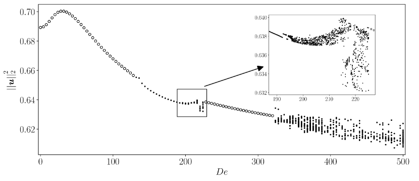
Figure 1: Filled circles: values of the squared 2-norm of the velocity vector at the instants when the Poincaré section is crossed. Open circles: values of the square of the 2-norm of the velocity vector in the stationary cases. The first bifurcation from a steady regime to an unsteady, periodic regime occurs at $De=128.32$. Starting from $De\approx 193$ we observe two periods which are incommensurable, characteristic of the aperiodic regime. Then the system quickly evolves into chaos from $De\approx 195$. For $De\in[227,318]$ the system is again stationary, after a narrow periodicity interval the system becomes again chaotic at $De=324$. A magnification of the bifurcation diagram for $De\in[190,230]$ is shown in the inset

By increasing the Dean number, we see that the system holds its periodicity until $De\approx 193$ (using the definition of $De$ in equation 5, which is not the same used in Wang and Yang [31, 27]), where it becomes aperiodic. Wang and Yang [31, 27] also saw a change in behaviour in that Dean number range, a slight increase and then a decrease in the period, but they did not mention to observe aperiodicity. This aperiodic regime is only observed over a narrow range of $De$, already at $De=195$ the system is complex enough to be considered as chaotic. Analysing the magnified part in figure 1, we notice the presence of a new solution branch to which the system abruptly jumps back and forth. The increase in complexity is then very rapid, between $De=125$ and $214$ the system is chaotic with values of the velocity norm that remain enclosed in the envelope of the two former branches. Between $De=214$ and $227$ the values no longer lie within the same envelope, probably due to the presence of a third branch (which was indeed observed by Wang and Yang [31]). For $De>227$ the system very quickly returns to a stationary regime, which lasts until $De=318$, where very mild, periodic oscillations are observed up to $De=323$. For higher Dean numbers the system rapidly becomes again chaotic, no stationary or periodic regimes were observed for higher Dean numbers.

The changes in regime observed for the present model are in very good agreement with the literature. In particular the critical Dean number given by the model, $De_{c}=128.32$, is in excellent accordance with the $De_{c}=128.22$ by Wang and Yang [31], which is one of the most accurate studies available, or $De_{c}=129.71$ by Winters [16]. Both these results were obtained by solving the full 2D Navier Stokes equations in polar coordinates without low curvature approximation, thus with two control parameters. The bifurcation to the new steady state occurs at $De=227$ with our model, which is slightly above the value obtained in Ref 31, $De=217$. The agreement is better for the next bifurcation to chaos, which is observed at $De=323$ for both models.

Nonetheless a difference is observed at the end of the stationary region: in the section between $De=318$ and $323$ our model produces slight periodic oscillations, while Wang and Yang [31] report an aperiodic oscillation from $De=312$ until the beginning of the chaotic region at $De=323$.

III.2 The periodic regime

Figure 2 shows the dependence of the oscillation period on $De$ in the periodic regime. The open circles represent the time intervals between two crossings of the Poincaré section, i.e. the period. As for figure 1, the symbols are the superposition of several circles, onto one position for a periodic signal, and two or more in the aperiodic or chaotic regime. At $De>193$ there is a progressive separation in two different set of circles, this identifies the aperiodicity seen in figure 1. Wang and Yang [31] report $T=0.159$ at $De=182.2$, retrieved with the full NS equations while the present model gives $T=0.1579$ at the same $De$. Between $De_{c}$ and $De=150$ the period dependence on $De$ follows the law:

$$T=\frac{1.013}{(De-De_{c})^{0.53}}$$

which is represented with a dashed curve in the figure and is close to a $-0.5$ power law in agreement with supercritical pitchfork bifurcation. In fact, the computed exponent approaches the theoretical value of $-0.5$ when the curve fitting is restricted to Dean numbers close to the critical value, in agreement with the weakly non linear framework for the theoretical $-0.5$ value.

The spectrum in figure 3 shows the amplitudes of the Fourier modes of the cross stream velocity $w$ measured at $y=0.9045,z=0.5$ at $De=130$, thus in the periodic regime. The spectrum was obtained by means of the FFT on a time series collected over 5 oscillation periods. The rapid exponential decrease of the amplitude of the modes with increasing pulsations indicates that the temporal dynamic in the periodic regime is dominated by the first oscillating mode.

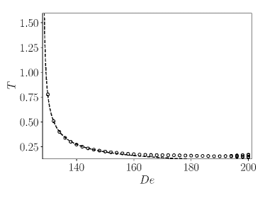
Figure 2: The oscillation period follows the law:
$T\propto(De-De_{c})^{\gamma}$, represented by dashed line, with $\gamma=0.53$, and $De_{c}=128.32$. Above $De\approx 193$ we observe the first part of aperiodic regime, which gives rise to higher complexity for higher $De$, see also figure 1.

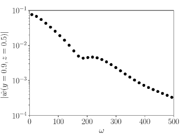
Figure 3: Cross stream velocity $w$ spectrum, $De=130$. The dynamics is dominated by the first mode, which corresponds to a period $T=0.7764$. Coherently with the observations and the symmetry of the problem, the zero mode vanishes in the spectrum, since the average $w$ is vanishing

The trajectory approaches and leaves periodically the vicinity of two equilibrium states, where the fluid’s dynamics slows down and its velocity fields resembles that of the equilibrium. These two equilibria are symmetric with respect to the spanwise direction (z) and are sometimes referred to as the 2 and 4 vortices solutions[7, 8, 16, 12]. The vector fields of these two solutions are shown on the left part of figure 4. However the 2 or 4 vortices classification can be misleading, because for $De>122.5$ the 2 vortices solution presents in truth 4 cells, even if the additional cells are much less intense than those observed in the 4 cell case. This was also observed by Watanabe and Yanase [32] who named the solutions the weak and the strong 4 vortices solutions. We will henceforth use this designation.

These streamwise vortices are the result of two different physical mechanisms. First, for confined curved flow, like in duct or pipe, the Coriolis acceleration ($-De\cdot u^{2}$ which is non-homogeneous in spanwise direction) is in equilibrium with the radial pressure gradient ($\partial p/\partial y$). As a consequence there is a spanwise pressure gradient ($\partial p/\partial z\neq 0$) which induces spanwise flow ($w\neq 0$). This mechanism is responsible of the so-called Dean vortices [1, 2, 3] which correspond to the 2-vortices steady solution mentioned above. Secondly, for a flow over a concave wall, when the wall-normal pressure gradient ($\partial p/\partial y$) is strong enough, it can give rise to streamwise counter-rotating vortices, this phenomenon is known as the Taylor-Görtler instability. The spanwise wavelength increases with the Reynolds number. The concomitance of these two mechanisms leads to the complexity mentioned above, with the observation of 4 strong or weak cells [32], and the possibility to observe 6 or more cells for higher Dean number.

Both the weak and strong 4 vortices steady solutions are observed even for subcritical Dean numbers. The strong 4-vortices solution is linearly unstable to non-symmetric perturbations (and stable otherwise)[16, 33], whereas for $De<De_{c}$ the weak 4 vortices solution is linearly stable.

This fact can be shown by performing linear stability analysis of those two equilibrium states at $De_{c}$. The NS equations are linearized around either of the steady state solutions and the perturbations can be expressed in the form

$${q^{\prime}}(y,z,t)=\sum_{n}Q_{n}(y,z)e^{\sigma_{n}t}$$ (7)

where $Q_{n}$ is the $n^{th}$ eigenmode associated to the eigenvalue $\sigma_{n}$. The real and imaginary parts of $\sigma$ are the growth rate and the pulsation, respectively. The equilibrium state is unstable if the real part of at least one $\sigma_{n}$ is positive and stable otherwise. The asymptotic behaviour is determined by the least stable mode. Numerically this least stable mode is calculated with

$$\sigma=\frac{1}{\int_{S}{q}^{*}q~{}dS}~{}\int_{S}{q}^{*}\frac{\partial q}{\partial t}~{}dS$$ (8)

(the $*$ denotes the complex conjugate) until convergence in the growth rate. The linear simulations are performed by imposing symmetry or anti-symmetry. Table 1 shows the eigenvalues of the most amplified mode for the weak and strong 4-vortices solutions and for symmetric and anti-symmetric perturbations. Alike in the literature previously mentioned, the strong 4 vortices solution is stable to symmetric perturbations and unstable to anti-symmetric ones. The weak 4-vortices solution is linearly stable to any perturbation in the subcritical regime.

Thus, when the system is non-symmetrically perturbed for $De<De_{c}$, it evolves close to the strong 4-vortices solution, which is a saddle point, thus the trajectory is ejected and the system eventually returns to the weak 4 cell solution, which is the global attractor. This is the reason why the latter is the observed solution in direct numerical simulation or experiments in the subcritical regime. When the system is non-symmetrically perturbed for $De>De_{c}$, the weak 4-vortices solution also becomes linearly unstable, a perturbation will therefore initiate a cycle between the two solutions. The periodic orbit of the system at $De=130$ is depicted in figure 4 in a state space diagram spanned with the energy injection and squared velocity 2-norm. The system follows the direction indicated by the small arrow in the center of the figure. Starting in the proximity of the weak 4 vortices solution (indicated with the black circle at the bottom left) the flow evolves towards the strong 4 vortices solution (indicated with the black square at the top left). The system then loses its symmetry, which is consistent with the instability to asymmetric perturbations of this solution. The two upper vortices collapse into one lateral vortex, producing a burst. The system then rapidly returns to a symmetric state, namely the weak 4 vortices solution.

The trajectory is attracted by the stable manifold (symmetric) of the strong 4-vortices equilibrium, it then leaves this region along the unstable manifold (antisymmetric) and heads to the second equilibrium state (weak 4-vortices). If $De>De_{c}$, then the trajectory follows the second heteroclinic orbit along the unstable manifold (symmetric) of the weak 4-vortices equilibrium, it then heads to the strong 4-vortices equilibrium state, closing the cycle. These two heteroclinic orbits between the two equilibria constitute a heteroclinic cycle which can be suppressed by imposing spanwise symmetry.

Table 1: Eigenvalue of the most unstable eigenmode of the strong and weak 4-vortices solutions at $De_{c}=128.32$, obtained by means of the linear stability analysis. The convergence was stopped when the change in value dropped below $10^{-4}$. The eigenvalues can be considered as real, in other words the pulsation is numerically zero.

	Symmetry	Antisymmetry
Strong 4 vortices	$-40.20+0i$	$+44.215-4.5\cdot 10^{-4}~{}i$
Weak 4 vortices	$-0.540-4.6\cdot 10^{-4}~{}i$	$-22.371-4.6\cdot 10^{-4}~{}i$

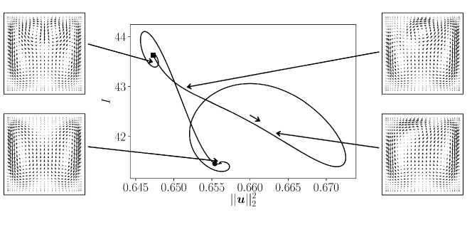
Figure 4: Injection-velocity norm phase diagram at $De=130$. The system follows a periodic orbit passing close to the 2 stationary solutions, indicated by the solid circle ($I\approx 41.5,||\bm{u}||_{2}^{2}\approx 0.655$) and the solid square (($I\approx 43.5,||\bm{u}||_{2}^{2}\approx 0.647$)). The long arrows indicate the instantaneous states of the system. The flow evolves following the small arrow: from the weak 4-cells, symmetric state to the symmetric strong 4-cells, when symmetry is broken a kinetic energy burst is observed. The system then returns to a weak 4-cells state regaining its symmetry.

III.3 High Dean regime, $\mathbf{De=10^{4}}$

The application of dynamical systems ideas to fluid mechanical problems has provided much insight into the ways fluids transit from a laminar state to a turbulent one. The identification of the different routes to chaos suggests they can also be routes to turbulence that lead from a laminar flow state through various bifurcations to a turbulent attractor. In this section we introduce a relatively high Dean number simulation, at $De=10^{4}$. The numerical parameters needed to be adapted $Ny=Nz=501$, $\Delta t=10^{-8}$. Figure 5 shows a snapshot of isocontours of the streamwise velocity $u$. As can be seen the topology changes drastically as compared to the 2 or 4 cells solutions observed so far at much lower Dean number (figure 4).

The solid no-slip walls are source of filament structures[34], which are advected away from the walls and disrupt the Dean vortices. While Dean vortices fill the whole domain, in other words they scale with the duct height $h$, the filament structures scale with the vorticity thickness at the wall. The ratio between these two length scales is related to the Dean number, thus for high Dean number we observe a multiscale dynamic leading to a complex spatio-temporal pattern. The 2D restriction is too strong to qualify this flow as realistically turbulent, nonetheless the richness of this minimal model permits to investigate turbulence within a dynamical system framework (see the recent discussion on the subject in Ref 35 and references therein).

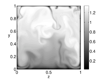
Figure 5: Isocontour of the streamwise velocity $u$. Snapshot of simulation at $De=10^{4}$

IV Conclusion and perspectives

In this paper we developed a simplified model for the flow in a weakly curved square duct, in line with the work by Dean [1]. However, while the original Dean model is based on a truncation at $\mathcal{O}(h/R)$, the present model is truncated at $\mathcal{O}(\sqrt{h/R})$, the square root comes from the use of two characteristic velocities. The simplified model is Cartesian and is governed by one control parameter, the numerical solution is therefore much simpler compared to the full Navier Stokes equations in polar coordinates. We compared the results with the literature [16, 31], finding a very good agreement in the bifurcation points and the oscillation period.

Moreover the model allowed us to investigate the periodic regime of the system in terms of both bifurcations and physical mechanisms, in addition, it was shown that the observed periodicity results of a heteroclinic cycle constituted by two heteroclinic orbits between the two equilibria: the weak and the strong 4-vortices solutions. The trajectory is backward asymptotic to one equilibrium state and forward asymptotic to the other and reciprocally on the way back closing a heteroclinic cycle.

The model is an example of deterministic chaos in fluid flows, as already seen in Rayleigh-Bénard convection or in Taylor-Couette flow between two rotating cylinders. Nonetheless these flows differ by the coupling term generating the streamwise vortices. In the present work this term is quadratic ($-De~{}u^{2}$) while it is linear in rotating or convective cases. This difference deserves investigations, and that was the original objective of the present paper. In that purpose, the complete program to solve 2D Navier-Stokes equations is made freely available.

Although presented in 2D in this paper, the present model was originally developed in 3D. In a future work we plan to extend our analysis to more complex flows, namely using the 3D version of the present model. A step was made in that direction by Ravi Sankar, Nandakumar, and Masliyah [36] for steady flows, and it appears interesting to continue towards more complex dynamics induced by turbulent inflow boundary conditions. In order to investigate the paradoxical effect of curvature: stabilising turbulence [19, 18, 17, 25] on one hand and generating peculiar streamwise vortices on the other hand.

Table 2: Comparison between two calculations at $De=150$, the quantities reported are averaged over one time period. The coarser space ($N$, number of grid points) and time discretisations (third line of the table) are those used in the rest of the paper, the finer simulation is used as a benchmark. Very little differences are observed in the results: the period $T$ varies of a quantity compatible with the $dt$ itself, the average pressure gradient $dP/dx$ and the streamwise and span wise dissipations $\varepsilon_{u}$,$\varepsilon_{vw}$ exhibit very limited differences. The differences between the streamwise pressure gradient (equal to the energy injection if $U_{b}=1$) and the streamwise dissipation indicate the level of convergence of the respective calculations.

$N_{y}\times N_{z}$	$\Delta t$	$T$	$dP/dx$	$\varepsilon_{u}$	$\varepsilon_{vw}$
$101\times 101$	$1\cdot 10^{-6}$	$0.20132$	$-44.5091$	$44.5066$	$11.43055$
$31\times 31$	$1.2\cdot 10^{-5}$	$0.2013$	$-44.513$	$44.5130$	$11.43557$

Appendix A The code

Equations (4) are solved using a solver based on Chebyshev collocation method. The time marching combines a fourth-order Adams-Bashforth scheme and a fourth-order backward differentiation scheme, with the viscous term treated implicitly [37].

The divergence-free condition is achieved with the prediction-projection scheme by Chorin and Temam (for an exhaustive review about projection methods see Ref 38). Pressure is computed using polynomials of 2 orders less than those used for the velocities, in order for the pressure field to remain unpolluted of spurious modes. The same grid is used for pressure and velocity fields and no pressure boundary condition is required. For further details on the accuracy and stability of the method see Ref 39. This numerical method was found to be accurate enough to compute the subcritical transition to turbulence in square duct flows[40]. Most of the results have been obtained with a grid composed of $Ny\times Nz=31\times 31$ Chebyshev points, with a time step ($\Delta t$) of $1.2\cdot 10^{-5}$. A quantitative comparison with a simulation performed using finer time step and grid can be found in table 2. The error in the oscillation period is of the same order of the time-step, the differences in the streamwise pressure gradient and streamwise and cross-stream dissipations averaged on one time period are below $5\%$, despite a more than ten-fold increase in the number of grid points and a 12-times finer time-step. The agreement between the average dissipation and pressure gradient in the streamwise direction testifies the convergence of the calculations.

Pages A.1 and A.2 contain the source code used to generate the data shown in the present paper. This version of the code mostly contains the calculating core of the program, while the most part of the post-processing was not included for clarity. Some quantities of interest are however added for validation purposes (the streamwise pressure gradient and the dissipations in streamwise direction and the dissipation in cross-flow directions $x$ and $y,z$-). The reader is encouraged to run the program and compare the results obtained with those reported in table 2. The simulation is initialized with the laminar solution plus a random velocity field, thus the initial transient shows a little sensitivity from run to run. The ’functions’ file is composed by four methods, inserted in a class for practicality. The ’constBulk’ method uses a bisection algorithm to iteratively calculate the streamwise pressure gradient required to maintain the target streamwise bulk velocity ($U_{b}=1$ in the present paper). The ’Chebyshev’ method is used to define the grid, the derivation matrices for velocity and pressure and the integration weights. The other two methods are auxiliaries for the ’Chebyshev’ method. The first part of the ’main’ file serves as initialization, here we define the operators for derivations and integrations in $y$ and $z$, the extrapolation ($c_{i},d_{i}$) and the time integration ($a_{1},b_{i}$) coefficients. Finally we set the initial condition with the laminar flow solution in a straight duct ($Ulam$), with some additional random noise.

The following part is the actual time loop. In the first part we compute the right-hand-side term (explicit) of the equations, then the solution is updated for the next time-steps before calculating the new predicted velocity field. This is then corrected to enforce the divergence free condition following the prediction-projection method by Chorin and Temam. As a last step of the loop the streamwise pressure gradient is calculated using the bisection method mentioned above, and the streamwise velocity is corrected as well.

The code is available for download in the online version of the paper, but can also be copy-pasted from the present $.pdf$ file and saved in two files: $main.py$ and $functions.py$, in the same folder. In this case particular attention must be paid on accurately copying the indentations, which are essential in a python program. The present results were obtained by running the program on a linux machine using the Anaconda distribution of python version 3.6.4. The code also works on python 2.7 (a test was run on the Anaconda distribution of python 2.7.16).

A.1 Main

import numpy as np

from functions import functions_cl as ff

De=150  ;   dt=1e-5

Ny = 31; Nz = Ny

#  Chebyshev collocation method, operators definition

cc=ff()

[Y,D1,D2,Dpy,WY]=cc.Chebyshev(Ny)

Y=(1-Y)/2; WY=-WY/2; D1=D1*2

y = Y[1:-1]; Wy = WY[1:-1]; Dy = -D1[1:Ny-1,1:Ny-1]; D2y = 4*D2[1:Ny-1,1:Ny-1]; Dpy=-2*Dpy; Ay = np.dot(Dy,Dpy)

[Ey_u,Qy_u] = np.linalg.eig(D2y); invQy_u=np.linalg.inv(Qy_u);  Ey_u=(np.tile(Ey_u, [Nz-2,1])).T

[Ey_p,Qy_p] = np.linalg.eig(Ay);  invQy_p=np.linalg.inv(Qy_p);  Ey_p=(np.tile(Ey_p, [Nz-2,1])).T

Dz=np.transpose(Dy); D2z=np.transpose(D2y); Dpz=np.transpose(Dpy); Az=np.transpose(Ay);

Qz_u=np.transpose(Qy_u);  invQz_u=np.transpose(invQy_u);  Ez_u=np.transpose(Ey_u);

Qz_p=np.transpose(Qy_p);  invQz_p=np.transpose(invQy_p);  Ez_p=np.transpose(Ey_p);

d1 = 4.;d2 = -6.;d3 = 4.;d4 = -1.                              # extrapolation coefficients

c1 = 2.;c2 = -1.;c3 = 0.;c4 = 0.                               # lower order for pressure

a1 = 25/12.;b1 = -4.;b2 = 3.;b3 = -4/3.;b4 = 1/4.;sig = a1/dt  # Backward Euler

# initializing flow field

Ulam =np.dot(np.dot( Qy_u,( np.dot (  np.dot( invQy_u,(-np.ones((Ny-2,Nz-2))) ) , invQz_u)/(Ey_u+Ez_u)) ),Qz_u)

Ulam = Ulam/( np.transpose(Wy).dot(Ulam).dot(Wy) )

Px=Wy.dot(Dy[0,:].dot(Ulam))*4

uf1=np.copy(Ulam)+np.random.rand(Ny-2,Ny-2)*1e-2; uf2=np.copy(uf1);uf3=np.copy(uf1);uf4=np.copy(uf1);

vf1=np.zeros((Ny-2,Ny-2)); vf2=np.copy(vf1); vf3=np.copy(vf1); vf4=np.copy(vf1)

wf1=np.zeros((Ny-2,Ny-2)); wf2=np.copy(wf1); wf3=np.copy(wf1); wf4=np.copy(wf1)

pf1=np.zeros((Ny-2,Ny-2)); pf2=np.copy(pf1); pf3=np.copy(pf1); pf4=np.copy(pf1)

timeEnd=1   ;k=0          ;U=np.zeros((Ny,Nz))

time=[0]    ;Px_time=[0]  ;V=np.zeros((Ny,Nz))

dissip_u=[0];dissip_vw=[0];W=np.zeros((Ny,Nz))

# ------------------------

#   starting time loop

while time[-1] < timeEnd:

    k+=1

    u=d1*uf1+d2*uf2+d3*uf3+d4*uf4

    v=d1*vf1+d2*vf2+d3*vf3+d4*vf4

    w=d1*wf1+d2*wf2+d3*wf3+d4*wf4

    p=c1*pf1+c2*pf2+c3*pf3+c4*pf4

    # -----  calculating right hand side  ----- #

    rhs_u = -( b1*uf1+b2*uf2+b3*uf3+b4*uf4 )/dt +De*(-v*(Dy.dot(u)) -w*(u.dot(Dz)))

    rhs_v = -( b1*vf1+b2*vf2+b3*vf3+b4*vf4 )/dt +De*(-v*(Dy.dot(v)) -w*(v.dot(Dz)) +u**2) - Dpy.dot(p)

    rhs_w = -( b1*wf1+b2*wf2+b3*wf3+b4*wf4 )/dt +De*(-v*(Dy.dot(w)) -w*(w.dot(Dz)))       - p.dot(Dpz)

    # ---------------  update  ---------------- #

    uf4=np.copy(uf3); uf3=np.copy(uf2); uf2=np.copy(uf1);

    vf4=np.copy(vf3); vf3=np.copy(vf2); vf2=np.copy(vf1);

    wf4=np.copy(wf3); wf3=np.copy(wf2); wf2=np.copy(wf1);

    pf4=np.copy(pf3); pf3=np.copy(pf2); pf2=np.copy(pf1);

    # -------------  prediction  ------------- #

    uf1 = Qy_u.dot( (invQy_u.dot(rhs_u).dot(invQz_u)) / (sig-Ey_u-Ez_u) ).dot(Qz_u)

    vf1 = Qy_u.dot( (invQy_u.dot(rhs_v).dot(invQz_u)) / (sig-Ey_u-Ez_u) ).dot(Qz_u)

    wf1 = Qy_u.dot( (invQy_u.dot(rhs_w).dot(invQz_u)) / (sig-Ey_u-Ez_u) ).dot(Qz_u)

    # -------------  projection  ------------- #

    div = Dy.dot(vf1)+wf1.dot(Dz)

    RHSP = sig*div + Ay.dot(p) + p.dot(Az)

    pf1 = Qy_p.dot( ((invQy_p.dot(RHSP)).dot(invQz_p))/(Ey_p+Ez_p)).dot(Qz_p)

    vf1 -=  1.0/sig*Dpy.dot((pf1-p))

    wf1 -=  1.0/sig*(pf1-p).dot(Dpz)

    Px = ff.constBulk(Px,Qy_u,invQy_u,Ey_u,Qz_u,invQz_u,Ez_u,sig,Wy,rhs_u)

    uf1 = np.dot( Qy_u,( ( np.dot( invQy_u,(rhs_u-Px ) ).dot(invQz_u) )/(sig-Ey_u-Ez_u) ) ).dot(Qz_u)

    if( k % 200  ) == 0:

      time.append(k*dt) ; Px_time.append(Px)

      # ------------------------  calculating dissipation  ------------------------ #

      # ----  derivative is non zero on boundary -> adding the implicit point  ---- #

      U[1:-1,1:-1]=u;   V[1:-1,1:-1]=v;   W[1:-1,1:-1]=w

      dissip_u.append(WY.dot((D1.dot(U))**2 + (U.dot(D1.T))**2).dot(WY) )

      dissip_vw.append(WY.dot((D1.dot(V))**2+(D1.dot(W))**2+(V.dot(D1.T))**2+(W.dot(D1.T))**2).dot(WY))

      # --------------------------------------------------------------------------- #

      divafter=Dy.dot(v)+w.dot(Dz)

      print(’time: ’+str(’%0.3f’%time[-1])+ ’ str-wise dissip:’+str(’%0.3f’%dissip_u[-1])+

              ’ div before/after proj: ’ +str(’%0.3e’%np.abs(div).max()) +’/’+

              str(’%0.3e’%np.abs(divafter).max()) +’ u bulk error:’+str(’%0.3e’%(Wy.dot(uf1).dot(Wy)-1)))

print(’average stream-wise dissipation: ’+str(’%0.5f’%(np.asarray( dissip_u [100:] ).mean())))

print(’average stream-wise press grad : ’+str(’%0.5f’%(np.asarray( Px_time  [100:] ).mean())))

print(’average span-wise   dissipation: ’+str(’%0.5f’%(np.asarray( dissip_vw[100:] ).mean())))

A.2 Functions

import numpy as np

class functions_cl:

    # ------------------------------------------

    # generation of grid and derivation matrices

    @staticmethod

    def cheb(N):

        if N == 0:

            D = 0

            x = 1

            ll=(D,x)

            return ll

        x = np.cos( np.pi*np.arange(N+1)/float(N) )

        c=np.ones(N+1)

        c[[0,-1]]=2

        c=c*(-1)**(np.arange(N+1))

        X = np.transpose(np.tile(x,[N+1,1]) )

        dX = X-np.transpose(X)

        # off-diagonal entries

        D  =  np.outer(c ,1/c) / (dX+np.eye(N+1))

        # diagonal entries

        D  = D -  np.diag(np.sum( np.transpose(D),0 ))

        return D,x

    @staticmethod

    def clencurt(N):

        # CLENCURT  nodes x (Chebyshev points) and weights w

        #           for Clenshaw-Curtis quadrature

        theta = np.pi*np.arange(N+1)/N

        w = np.zeros(N+1)

        ii = range(1,N)

        v = np.ones(N-1)

        if np.mod(N,2)==0:

            w[0] = 1./(N**2-1)

            w[N] = w[0]

            for k in np.arange (1,N/2):

              v = v - 2*np.cos(2*k*theta[ii])/(4*k**2-1)

            v = v - np.cos(N*theta[ii])/(N**2-1)

        else:

            w[0] = 1./N**2

            w[N] = w[0]

            for k in np.arange (1,(N-1)/2+1):

                v = v -    2*np.cos(2*k*theta[ii])  /  (4*k**2-1)

        w[ii] = 2.*v/N

        return w

    def Chebyshev(self,Ny):

        [Dy,y] = self.cheb(Ny-1)

        D2y = np.dot(Dy,Dy)

        Wy = self.clencurt(Ny-1)

        #Wy = ChebyshevCl.clencurt(Ny-1)

        #  see Botella, Dpy : derivative matrix without implicit BC

        c = (np.sin(  np.pi*(np.arange(1,Ny-1))/(Ny-1)    )**2) *(-1) ** np.arange(1,Ny-1)

        X = np.transpose(np.tile(y[1:Ny-1],[Ny-2,1]))

        dX = X-np.transpose(X)

        # off-diagonal entries

        D0 = np.outer((1./c),c)/(dX+(np.eye(Ny-2)))

        # diagonal entries

        Dpy = D0 - np.diag(np.sum(D0,1))

        return (y,Dy,D2y,Dpy,Wy)

    # -----------------------------------

    #   Bisection method for mean flow

    @staticmethod

    def constBulk(Px,Qy_u,invQy_u,Ey_u,Qz_u,invQz_u,Ez_u,sig,Wy,rhs_u):

        Px1=Px-.2;  uf1 = np.dot( Qy_u.dot( ( invQy_u.dot(rhs_u-Px) ) ).dot(invQz_u)/(sig-Ey_u-Ez_u) , Qz_u);

        Q1=np.dot(np.dot(Wy,uf1),Wy);

        Px2=Px+.2;  uf1 = np.dot( Qy_u.dot( ( invQy_u.dot(rhs_u-Px) ) ).dot(invQz_u)/(sig-Ey_u-Ez_u) , Qz_u);

        Q2=np.dot(np.dot(Wy,uf1),Wy);

        iter=1; Q=(Q2+Q1)/2;

        while abs(Q-1) > 1e-14:

            Px = (Px1+Px2)/2;

            uf1 = np.dot( Qy_u.dot( (invQy_u.dot((rhs_u-Px)) ).dot(invQz_u) / (sig-Ey_u-Ez_u) ) , Qz_u )

            Q=np.dot( np.dot(Wy,uf1),Wy )

            if Q>1:

                Px1=Px

            else:

                Px2=Px

            iter+=1

            if iter >=300:

                break

        return Px

References

- Dean [1927] W. Dean, “Xvi. note on the motion of fluid in a curved pipe,” The London, Edinburgh, and Dublin Philosophical Magazine and Journal of Science 4, 208–223 (1927), https://doi.org/10.1080/14786440708564324 .
- Dean [1928] W. Dean, “LXXII. the stream-line motion of fluid in a curved pipe (second paper),” The London, Edinburgh, and Dublin Philosophical Magazine and Journal of Science 5, 673–695 (1928), https://doi.org/10.1080/14786440408564513 .
- Dean and Hurst [1959] W. R. Dean and J. M. Hurst, “Note on the motion of fluid in a curved pipe,” Mathematika 6, 77–85 (1959).
- Eustice and Larmor [1910] J. Eustice and J. Larmor, “Flow of water in curved pipes,” Proceedings of the Royal Society of London. Series A, Containing Papers of a Mathematical and Physical Character 84, 107–118 (1910), https://royalsocietypublishing.org/doi/pdf/10.1098/rspa.1910.0061 .
- McConalogue and Srivastava [1968] D. J. McConalogue and R. S. . Srivastava, “Motion of a fluid in a curved tube,” Proceedings of the Royal Society of London. Series A. Mathematical and Physical Sciences 307, 37–53 (1968), https://royalsocietypublishing.org/doi/pdf/10.1098/rspa.1968.0173 .
- Van Dyke [1978] M. Van Dyke, “Extended Stokes series: laminar flow through a loosely coiled pipe,” Journal of Fluid Mechanics 86, 129–145 (1978).
- Cheng and Akiyama [1970] K. Cheng and M. Akiyama, “Laminar forced convection heat transfer in curved rectangular channels,” International Journal of Heat and Mass Transfer 13, 471–490 (1970).
- Joseph, Smith, and Adler [1975] B. Joseph, E. P. Smith, and R. J. Adler, “Numerical treatment of laminar flow in helically coiled tubes of square cross section. part I. stationary helically coiled tubes,” AIChE Journal 21, 965–974 (1975), https://onlinelibrary.wiley.com/doi/pdf/10.1002/aic.690210519 .
- Cheng, Lin, and Ou [1976] K. C. Cheng, R. C. Lin, and J. W. Ou, “Fully developed laminar flow in curved rectangular channels,” Journal of Fluids Engineering, Transactions of the ASME 98, 41–48 (1976).
- Dennis and NG [1982] S. Dennis and M. NG, “Dual solutions for steady laminar flow through a curved tube,” The Quarterly Journal of Mechanics and Applied Mathematics 35, 305–324 (1982).
- Daskopoulos and Lenhoff [1989] P. Daskopoulos and A. Lenhoff, “Flow in curved ducts: bifurcation structure for stationary ducts,” Journal of Fluid Mechanics 203, 125–148 (1989).
- Yanase, Goto, and Yamamoto [1989] S. Yanase, N. Goto, and K. Yamamoto, “Dual solutions of the flow through a curved tube,” Fluid Dynamics Research 5, 191 – 201 (1989).
- Shanthini and Nandakumar [1986] R. Shanthini and K. Nandakumar, “Bifurcation phenomena of generalized Newtonian fluids in curved rectangular ducts,” Journal of Non-newtonian Fluid Mechanics 22, 35–60 (1986).
- Ito [1969] H. Ito, “Laminar flow in curved pipes,” ZAMM - Journal of Applied Mathematics and Mechanics / Zeitschrift für Angewandte Mathematik und Mechanik 49, 653–663 (1969), https://onlinelibrary.wiley.com/doi/pdf/10.1002/zamm.19690491104 .
- Berger, Talbot, and Yao [1983] S. A. Berger, L. Talbot, and L. S. Yao, “Flow in curved pipes,” Annual Review of Fluid Mechanics 15, 461–512 (1983), https://doi.org/10.1146/annurev.fl.15.010183.002333 .
- Winters [1987] K. H. Winters, “A bifurcation study of laminar flow in a curved tube of rectangular cross-section,” Journal of Fluid Mechanics 180, 343–369 (1987).
- White and Appleton [1929] C. M. White and E. V. Appleton, “Streamline flow through curved pipes,” Proceedings of the Royal Society of London. Series A, Containing Papers of a Mathematical and Physical Character 123, 645–663 (1929), https://royalsocietypublishing.org/doi/pdf/10.1098/rspa.1929.0089 .
- Taylor [1929] G. I. Taylor, “The criterion for turbulence in curved pipes,” Proceedings of the Royal Society of London. Series A, Containing Papers of a Mathematical and Physical Character 124, 243–249 (1929), https://royalsocietypublishing.org/doi/pdf/10.1098/rspa.1929.0111 .
- Sreenivasan and Strykowski [1983] K. R. Sreenivasan and P. J. Strykowski, “Stabilization effects in flow through helically coiled pipes,” Experiments in Fluids 1, 31–36 (1983).
- Rinaldi, Canton, and Schlatter [2019] E. Rinaldi, J. Canton, and P. Schlatter, “The vanishing of strong turbulent fronts in bent pipes,” Journal of Fluid Mechanics 866, 487–502 (2019).
- Canton, Schlatter, and Örlü [2016] J. Canton, P. Schlatter, and R. Örlü, “Modal instability of the flow in a toroidal pipe,” Journal of Fluid Mechanics 792, 894–909 (2016).
- Kühnen et al. [2015] J. Kühnen, P. Braunshier, M. Schwegel, H. C. Kuhlmann, and B. Hof, “Subcritical versus supercritical transition to turbulence in curved pipes,” Journal of Fluid Mechanics 770, R3 (2015).
- Kühnen et al. [2014] J. Kühnen, M. Holzner, B. Hof, and H. C. Kuhlmann, “Experimental investigation of transitional flow in a toroidal pipe,” Journal of Fluid Mechanics 738, 463–491 (2014).
- Barkley [2019] D. Barkley, “Taming turbulent fronts by bending pipes,” Journal of Fluid Mechanics 872, 1–4 (2019).
- Kalpakli Vester, Örlü, and Alfredsson [2016] A. Kalpakli Vester, R. Örlü, and P. H. Alfredsson, “Turbulent Flows in Curved Pipes: Recent Advances in Experiments and Simulations,” Applied Mechanics Reviews 68 (2016), 10.1115/1.4034135, https://asmedigitalcollection.asme.org/appliedmechanicsreviews/article-pdf/68/5/050802/4441856/amr_068_05_050802.pdf .
- Mondal et al. [2007] R. N. Mondal, Y. Kaga, T. Hyakutake, and S. Yanase, “Bifurcation diagram for two-dimensional steady flow and unsteady solutions in a curved square duct,” Fluid Dynamics Research 39, 413 (2007).
- Wang and Yang [2005] L. Wang and T. Yang, “Periodic oscillation in curved duct flows,” Physica D: Nonlinear Phenomena 200, 296 – 302 (2005).
- Yanase, Watanabe, and Hyakutake [2008] S. Yanase, T. Watanabe, and T. Hyakutake, “Traveling-wave solutions of the flow in a curved-square duct,” Physics of Fluids 20, 124101 (2008), https://doi.org/10.1063/1.3029703 .
- Mees, Nandakumar, and Masliyah [1996a] P. A. J. Mees, K. Nandakumar, and J. H. Masliyah, “Steady spatial oscillations in a curved duct of square cross-section,” Physics of Fluids 8, 3264–3270 (1996a), https://doi.org/10.1063/1.869108 .
- Mees, Nandakumar, and Masliyah [1996b] P. A. J. Mees, K. Nandakumar, and J. H. Masliyah, “Secondary instability of flow in a curved duct of square cross-section,” Journal of Fluid Mechanics 323, 387–409 (1996b).
- Wang and Yang [2004] L. Wang and T. Yang, “Bifurcation and stability of forced convection in curved ducts of square cross-section,” International Journal of Heat and Mass Transfer 47, 2971 – 2987 (2004).
- Watanabe and Yanase [2013] T. Watanabe and S. Yanase, “Bifurcation study of three-dimensional solutions of the curved square-duct flow,” Journal of the Physical Society of Japan 82, 074402 (2013), https://doi.org/10.7566/JPSJ.82.074402 .
- Bara, Nandakumar, and Masliyah [1992] B. Bara, K. Nandakumar, and J. H. Masliyah, “An experimental and numerical study of the Dean problem: flow development towards two-dimensional multiple solutions,” Journal of Fluid Mechanics 244, 339–376 (1992).
- Clercx and van Heijst [2009] H. J. H. Clercx and G. J. F. van Heijst, “Two-dimensional Navier-Stokes turbulence in bounded domains,” Applied Mechanics Reviews 62 (2009), 10.1115/1.3077489, https://asmedigitalcollection.asme.org/appliedmechanicsreviews/article-pdf/62/2/020802/4721117/020802_1.pdf .
- Hof and Budanur [2017] B. Hof and N. B. Budanur, “Searching for order in turbulent flow,” Physics 10, 25 (2017).
- Ravi Sankar, Nandakumar, and Masliyah [1988] S. Ravi Sankar, K. Nandakumar, and J. H. Masliyah, “Oscillatory flows in coiled square ducts,” The Physics of Fluids 31, 1348–1359 (1988), https://aip.scitation.org/doi/pdf/10.1063/1.866728 .
- Ascher, Ruuth, and Wetton [1995] U. Ascher, S. Ruuth, and B. Wetton, “Implicit-explicit methods for time-dependent partial differential equations,” SIAM Journal on Numerical Analysis 32, 797–823 (1995), https://doi.org/10.1137/0732037 .
- Guermond, Minev, and Shen [2006] J. Guermond, P. Minev, and J. Shen, “An overview of projection methods for incompressible flows,” Computer Methods in Applied Mechanics and Engineering 195, 6011 – 6045 (2006).
- Botella [1997] O. Botella, “On the solution of the Navier-Stokes equations using Chebyshev projection schemes with third-order accuracy in time,” Computers and Fluids 26, 107 – 116 (1997).
- Biau and Bottaro [2009] D. Biau and A. Bottaro, “An optimal path to transition in a duct,” Philosophical Transactions of the Royal Society A: Mathematical, Physical and Engineering Sciences 367, 529–544 (2009), https://royalsocietypublishing.org/doi/pdf/10.1098/rsta.2008.0191 .