Scaling law of transient lifetime of chimera states under dimension-augmenting perturbations

Abstract

Chimera states arising in the classic Kuramoto system of two-dimensional phase coupled oscillators are transient but they are “long” transients in the sense that the average transient lifetime grows exponentially with the system size. For reasonably large systems, e.g., those consisting of a few hundreds oscillators, it is infeasible to numerically calculate or experimentally measure the average lifetime, so the chimera states are practically permanent. We find that small perturbations in the third dimension, which make system “slightly” three-dimensional, will reduce dramatically the transient lifetime. In particular, under such a perturbation, the practically infinite average transient lifetime will become extremely short, because it scales with the magnitude of the perturbation only logarithmically. Physically, this means that a reduction in the perturbation strength over many orders of magnitude, insofar as it is not zero, would result in only an incremental increase in the lifetime. The uncovered type of fragility of chimera states raises concerns about their observability in physical systems.

I Introduction

A research frontier in complex and nonlinear dynamical systems is chimera states Umberger et al. (1989); Kuramoto and Battogtokh (2002); Abrams and Strogatz (2004); Shima and Kuramoto (2004); Abrams and Strogatz (2006); Abrams et al. (2008); Sethia et al. (2008); Laing (2009); Sheeba et al. (2009); Martens (2010); Martens et al. (2010); Omel’chenko et al. (2010); Wolfrum and Omel’chenko (2011); Wolfrum et al. (2011); Omelchenko et al. (2011); Omel’chenko et al. (2012); Zhu et al. (2012); Laing et al. (2012); Tinsley et al. (2012); Hagerstrom et al. (2012); Omelchenko et al. (2013); Ujjwal and Ramaswamy (2013); Zhu et al. (2013); Yao et al. (2013); Nkomo et al. (2013); Martens et al. (2013); Larger et al. (2013); Panaggio and Abrams (2013); Gu et al. (2013); Sieber et al. (2014); Schmidt et al. (2014); Zhu et al. (2014); Omel’chenko (2013); Omel’chenko et al. (2008); Xie et al. (2014); Yao et al. (2015); Maistrenko et al. (2015); Panaggio and Abrams (2015a, b); Martens and Bick (2015); Omelchenko et al. (2015a); Böhm et al. (2015); Nkomo et al. (2016); Viennot and Aubourg (2016); Hart et al. (2016); Gambuzza and Frasca (2016); Semenov et al. (2016); Kemeth et al. (2016); Ulonskaa et al. (2016); Hart et al. (2016); Andrzejak et al. (2017); Bera et al. (2017); Rakshit et al. (2017); Semenova et al. (2017); Malchow et al. (2018); Botha and Kolahchi (2018); Omelchenko et al. (2018); Xu et al. (2018); Yao et al. (2019), a phenomenon of spontaneous symmetry breaking in spatially extended systems in which coherent and incoherent groups of oscillators coexist simultaneously. The phenomenon was first observed three decades ago in a numerical study of the system of coupled nonlinear Duffing oscillators Umberger et al. (1989), which was later rediscovered Kuramoto and Battogtokh (2002), analyzed and coined with the term “chimera” Abrams and Strogatz (2004); Shima and Kuramoto (2004). Chimera states have been studied in diverse systems such as regular networks of phase-coupled oscillators with a ring topology Kuramoto and Battogtokh (2002); Abrams and Strogatz (2004, 2006), networks hosting a few populations Abrams et al. (2008); Martens (2010), two-dimensional (2D) Shima and Kuramoto (2004); Martens et al. (2010) and three-dimensional (3D) lattices Maistrenko et al. (2015), torus Panaggio and Abrams (2013); Omel’chenko et al. (2012), and systems with a spherical topology Panaggio and Abrams (2015a). Phenomena such as traveling-wave type of chimera Xie et al. (2014) and amplitude chimera Böhm et al. (2015); Hart et al. (2016) have also been uncovered and studied.

In the Kuramoto model with 2D rotational dynamics, a previous study Wolfrum and Omel’chenko (2011) demonstrated that the chimera states are typically transient. These states were deemed “long transient” because their average lifetime increases exponentially with the system size. For systems of size greater than, say, 60, it is already infeasible to numerically calculate the average transient time. For larger systems consisting of, e.g., a few hundreds oscillators, the average transient lifetime is practically infinite. The questions to be addressed in this paper are whether the practically infinitely long transient will become short so that the chimera states are actually transient from the standpoint of numerical computations or physical experiments when external perturbations are applied to the system, and how. Previous work focused mostly on perturbations to the structure of the underlying lattice or networks Yao et al. (2013); Omelchenko et al. (2015b); Malchow et al. (2018), revealing that chimera states are robust against structural perturbations. For example, when some links are removed from an originally globally coupled (all-to-all) network, coherent and incoherent regions still simultaneously arise in the state space, giving rise to a generalized type of chimera states Yao et al. (2013). Quite recently, it was found that a chimera state can respond to perturbations to achieve robustness through the mechanism of self-organization and adaptation Yao et al. (2019).

In this paper, we report an unexpected type of fragility of chimera states in the presence of perturbations to the phase-space dimension of the oscillators in the network. We start from the paradigmatic Kuramoto model of globally coupled 2D phase oscillators Kuramoto and Battogtokh (2002); Abrams and Strogatz (2004). In this model, each oscillator is a 2D rotor characterized by a single dynamical variable, the angle of planar rotation. We invoke arbitrarily small perturbations that make the oscillator “slightly” 3D. Specifically, consider 3D rotation represented by the movement of a point on the surface of a unit sphere $S^{2}$, where 2D rotation of the unperturbed phase oscillator is confined to movements on the equator. We find that any infinitesimal deviation from the equator in the oscillator dynamics makes the long-transient chimera state extremely short. In particular, let $\delta$ be the strength of this kind of “dimension-augmenting” perturbation. We find that, regardless of how infinitesimal $\delta$ is, insofar as its value is not zero, the average transient lifetime $\langle\tau\rangle$ of the chimera states becomes extremely short as it depends only logarithmically on $\delta$: $\langle\tau\rangle\sim-\ln{\delta}$, even for large systems for which the average transient lifetime in 2D is practically infinite. The physical significance is that, when the strength of the perturbation is reduced by many orders of magnitude, the average transient lifetime would incur only an incremental increase. Considering that in many existing studies of chimera states, whether it be physical, chemical or biological, a description based on Kuramoto type of 2D rotors is only approximate and perturbations that alter the 2D picture are inevitable, our finding raises concerns about the physical observability of chimera states.

It should be noted that, in this paper, an $N$-dimensional chimera state for $N\geq 3$ is defined as one that emerges in the full $N$-dimensional phase space as the result of dimension-augmenting perturbations. Because the focus of our study is on the transient nature of such high-dimensional chimera states, we set the initial condition to be a chimera state in two dimensions as in the classical Kuramoto model and examine how long the state can survive under such perturbations. This is done for two cases: the perturbations are such that the local phase space of each oscillator becomes three- or four-dimensional, respectively. We also note that a previous work Loos et al. (2016) revealed a logarithmic dependence of the average lifetime of transient chimera states on the intensity of Gaussian white noise, indicating a dramatic reduction of the chimera lifetime under noise. Our finding of a similar scaling law but with respect to deterministic, dimension-augmenting perturbations is further indication of the fragility of chimera states.

II Model

II.1 General consideration

We begin with the following $D$-dimensional Kuramoto model Olfati-Saber (2006); Lohe (2009); Chandra et al. (2019a, b):

$$\frac{d\bm{\sigma}_{i}}{dt}=\frac{K}{N}\sum_{j=1}^{N}\left[\bm{\sigma}_{j}-\left(\bm{\sigma}_{j}\cdot\bm{\sigma}_{i}\right)\bm{\sigma}_{i}\right]+\bm{{\rm W}}\cdot\bm{\sigma}_{i},$$ (1)

where the $D$-dimensional unit vector $\bm{\sigma}_{i}$ represents the state of the $i$th oscillator, $\bm{W}$ is a real $D\times D$ antisymmetric matrix characterizing the natural rotation of the oscillator, and $N$ is the system size (the number of coupled oscillators). The state of each node has $\left(D-1\right)$ degrees of freedom. For $D=2$, the system reduces to the classic Kuramoto model with the variable substitution $\bm{\sigma}_{i}=\left(\cos{\theta_{i}},\sin{\theta_{i}}\right)$. In Eq. (1), global (all-to-all) coupling is assumed, which is idealized. In a realistic situation, coupling is neither global nor highly local. We thus consider the following generalized model:

$$\frac{d\bm{\sigma}_{i}}{dt} = \frac{1}{N}\sum_{j=1}^{N}G\left(i-j\right)\left[\bm{{\rm T}}\cdot\bm{\sigma}_{j}-\left((\bm{{\rm T}\cdot\sigma}_{j})\cdot\bm{\sigma}_{i}\right)\bm{\sigma}_{i}\right]$$ (2)

$$+ \bm{{\rm W}}\cdot\bm{\sigma}_{i},$$

where $G\left(i-j\right)$ is a coupling function of a finite range, e.g., $G\left(i-j\right)=1+A\cos{\left[2\pi\left(i-j\right)/N\right]}$, and $\bm{{\rm T}}$ is a $D\times D$ isometric matrix taking into account phase lag. The oscillators can be visualized to be located on a ring and the coupling strength between a pair of nodes decreases with their distance according to $G(i-j)$. The state vector $\bm{\sigma}_{i}$ is now a high-dimensional unit vector. Let the starting point of $\bm{\sigma}_{i}$ be the origin so its ending point is on the surface of the high-dimensional unit sphere. In 3D the system can be conceived as a “pearl necklace,” as shown in Fig. 1(a), where $\bm{\sigma}_{i}$ of each oscillator moves on the surface of its pearl and all the pearls are located on the ring.

In 2D, the isometric matrix $\bm{{\rm T}}$ reduces to the standard rotation matrix of angle $\alpha$ as

$$\bm{{\rm T}}=\begin{bmatrix}\cos\alpha&\sin\alpha\\ -\sin\alpha&\cos\alpha\\ \end{bmatrix}.$$ (3)

While acting on a vector, T alters its direction while preserving its length, thus serves as a phase lag. Given an isometry in $d$ dimensions, there exists a reference framework in which $\bm{{\rm T}}$ can be written in the form

$$\bm{{\rm T}}=\begin{bmatrix}\bm{{\rm PR_{1}}}\\ &\bm{{\rm PR_{2}}}\\ &&{...}\\ &&&\bm{{\rm PR_{k}}}\\ &&&&\bm{{\rm RF_{m}}}\\ &&&&&\bm{{\rm I_{d-2k-m}}}\end{bmatrix},$$ (4)

where $\bm{{\rm PR_{i}}}$ ($i=1,2...k$) is the proper rotation matrix in 2D:

$$\bm{{\rm PR_{i}}}=\begin{bmatrix}\cos\alpha_{i}&\sin\alpha_{i}\\ -\sin\alpha_{i}&\cos\alpha_{i}\\ \end{bmatrix},$$ (5)

$\bm{{\rm I_{d-2k-m}}}$ is the$(d-2k-m)\times(d-2k-m)$ identity matrix, and $\bm{{\rm RF_{m}}}$ is the $m\times m$ reflection matrix with all the diagonal elements $-1$ and all the off-diagonal elements zero: $\bm{{\rm RF_{m}}}=-\bm{{\rm I_{m}}}$. We can use the three integers above: $d$, $k$ and $m$, to classify all different types of isometry subject to the constraint $d\geq 2k+m$. We impose another constraint: $k\geq 1$, to ensure a finite phase lag.

For $d=2$, the only choice is $k=1$ and $m=0$, which is simply the 2D proper rotation matrix. For $d=3$, it is necessary to choose $k=1$, and $m$ can be either $1$ or $-1$. We study both cases. For $d=4$, we have four different choices: (1) $k=2$ and $m=0$, (2) $k=1$ and $m=0$, (3) $k=1$ and $m=1$, and (4) $k=1$ and $m=2$.

With the following space and time dependent order parameter: $\bm{\rho}_{i}=N^{-1}\sum_{j=1}^{N}G\left(i-j\right)\bm{\sigma}_{j}$, we rewrite our generalized $D$-dimensional Kuramoto model as

$$d\bm{\sigma}_{i}/dt=\bm{{\rm T}\rho}_{i}-\left(\bm{{\rm T}\rho}_{i}\cdot\bm{\sigma}_{i}\right)\bm{\sigma}_{i}+\bm{{\rm W}}\bm{\sigma}_{i}.$$ (6)

II.2 Articulation of dimension-augmenting perturbations

To be concrete, we focus on perturbations that make the system 3D. To investigate the lifetime of chimera states, we articulate a scheme such that the 2D chimera states are a natural solution of the system. We then perturb this solution into 3D and determine whether or not it is still a long transient. (It should be emphasized that, without any perturbation, given the symmetry of the system about the $(x,y)$-plane, the system would remain 2D, and all the results would be the same as for the 2D system.)

More specifically, for vector rotation on a sphere, there are two independent dynamical variables: the longitudinal and latitudinal angles. For a network of size $N$, the phase space dimension is thus $2N$. For oscillator $i$, let $0\leq\theta_{i}<2\pi$ and $-\pi/2\leq\gamma_{i}\leq\pi/2$ be the longitudinal and latitudinal angles, respectively. To make the $N$-dimensional subspace defined by $\gamma_{i}=0$ ($i=1,\ldots,N$) an invariant subspace of the system, we choose a frame in which the initial 2D plane is the plane containing the equator and set the $z$-axis of the frame to be the axis of the proper rotation component of $\bm{{\rm T}}$. In this frame, the isometric matrix $\bm{{\rm T}}$ is:

$$\bm{{\rm T}}=\begin{bmatrix}\cos{\alpha}&\sin{\alpha}&0\\ -\sin{\alpha}&\cos{\alpha}&0\\ 0&0&T_{33}\end{bmatrix},$$ (7)

According to our definition of $\bm{{\rm T}}$ in Sec. II, $T_{33}$ can be either $1$ or $-1$, corresponding to whether a reflection symmetry is excluded or included, respectively. For $T_{33}=1$, no chimera state can arise because the system dynamics are such that all oscillators quickly synchronize to the fixed points of the transformation $\bm{{\rm T}}$: $(0,0,\pm 1)$ (in the Cartesian coordinates). We thus focus on the case $T_{33}=-1$ here and treat the case $T_{33}=1$ in Sec. V.

We make the natural rotation $\bm{{\rm W}}$ about the $z$-axis, so the system degenerates to 2D in the absence of any perturbation. In this case, $\bm{{\rm W}}$ plays no role in the dynamics, since it can be removed by setting the reference frame to one rotating about the z-axis at the same frequency. These considerations lead us to rewrite the general system equation Eq.(6) in the spherical coordinate as

$$\frac{d\theta_{i}}{dt} = -R_{i}\frac{\cos\Gamma_{i}}{\cos\gamma_{i}}\sin\left(\theta_{i}-\Theta_{i}+\alpha\right)$$ (8)

$$\frac{d\gamma_{i}}{dt} = -R_{i}\times[\cos\left(\theta_{i}-\Theta_{i}+\alpha\right)\sin\gamma_{i}\cos\Gamma_{i}$$ (9)

$$- T_{33}\cos\gamma_{i}\sin\Gamma_{i}]$$

where $\Theta_{i}$, $\Gamma_{i}$ and $R_{i}$ are the longitudinal angle, latitudinal angle and the length of the order parameter $\bm{\rho}_{i}$ at the location of the $i$th oscillator, respectively. Note that, in 2D, the equation for the single dynamical variable $\theta_{i}$ is

$$d\theta_{i}/dt=-R_{i}\sin\left(\theta_{i}-\Theta_{i}+\alpha\right).$$

Comparing this with Eq. (8), we see that the extra factor in 3D is

$$\chi_{i}\equiv\cos\Gamma_{i}/\cos\gamma_{i},$$ (10)

which we name as the dimensionality measure. For $\gamma_{i}=0$ ($i=1,\ldots,N$), we have $\Gamma_{i}=0$ and $\chi_{i}=1$, so Eq. (8) reduces to the 2D form, meaning that the 2D chimera states are an invariant solution of the 3D system.

III Scaling results

III.1 Logarithmic scaling of average transient lifetime of chimera states with dimension-augmenting perturbation in 3D

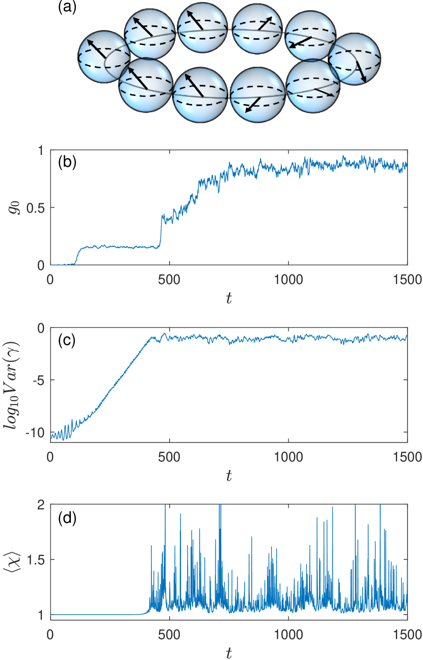
Figure 1: System illustration and transient chimera states in 3D. (a) The system can be conceived as a “pearl necklace” with each oscillator oscillating on the surface of its $3D$ “pearl” and all the pearls being located on a ring. (b) Time evolution of $g_{0}\left(t\right)$. The time interval in which the relative size $g_{0}\left(t\right)$ of the coherent region in space is approximately constant indicates the existence of a chimera state. Variations in $g_{0}\left(t\right)$ arise for $t>459$, signifying the disappearance of the 2D-like chimera state. (c) Evolution of $\mbox{Var}(\gamma)$, the variance of $\gamma$, which increases approximately exponentially during the transient 2D-like chimera state and reaches a plateau a short time before the collapse of the 2D-like structure. (d) Time evolution of the space averaged dimensionality measure $\langle\chi_{i}\rangle$ in Eq. (8). For $t\lesssim 400$, the value of $\langle\chi_{i}\rangle$ remains at one, indicating that the network dynamics are essentially of the 2D Kuramoto type. Parameter values are $N=400$, $T_{33}=-1$, $\delta=0.0001$, $A=0.995$, and $\alpha=\pi/2-0.05$. We use this pair of values of $A$ and $\alpha$ because the basin of the 2D chimera state is relatively large, facilitating numerical simulations.

A previous study Wolfrum and Omel’chenko (2011) of the 2D version of Eq. (6) indicated the existence of transient chimera states with a long lifetime. The transient time increases exponentially with the system size $N$, making numerical simulations infeasible to observe the collapse of the chimera state for, e.g., $N>60$. Our question is whether the chimera states can sustain such a long lifetime when the 2D system is perturbed into a higher-dimensional one.

To detect possible chimera states in 3D, we calculate the discrete Laplacian $D_{i}$ at node $i$ as a measure of the spatial coherence and derive the relative size $g_{0}$ of the coherence region in the space Kemeth et al. (2016). We then calculate the time evolution of $g_{0}$ and the instantaneous distributions of $D_{i}$. A finite time interval in which $g_{0}$ is approximately constant while the distribution of $D_{i}$ has two peaks signifies the existence of a transient chimera state (Appendix A). Figure 1(b) shows a typical behavior of the time evolution of $g_{0}$, where its value increases from zero initially and reaches a plateau at $t\approx 120$. For $120\lesssim t\lesssim 460$, $g_{0}$ is constant. For $t\gtrsim 460$, the value of $g_{0}$ increases continuously, indicating a deterioration of the chimera state and system’s approaching a global, loosely synchronous state (Sec. IV).

The transient nature of the observed chimera state can be understood, as follows. Start from a random set of 2D initial conditions for the oscillators, i.e., $\gamma_{i}(0)=0$. Without any perturbation, the system dynamics remain 2D with $\gamma_{i}(t)=0$ for all $t$. In this case, chimera states of long duration can arise insofar as the system size is not too small Wolfrum and Omel’chenko (2011). However, with a small perturbation to the latitudinal angle of a single oscillator in the initial condition, e.g., $\delta=10^{-3}$ in Fig. 1(b), the system will remain to be approximately 2D for only a finite amount of time, which can be seen from the behaviors of the space averaged values of the variance of $\gamma_{i}$ and of the dimensionality measure $\langle\chi_{i}\rangle(t)$, as shown in Figs. 1(c) and 1(d), respectively. These results demonstrate that, for $t\lesssim 450$, the dynamics of the oscillators are effectively 2D but they become 3D afterwards.

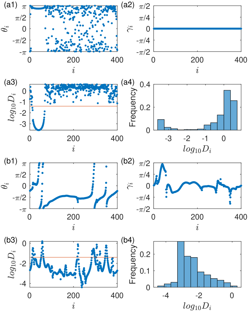
Figure 2: Visualization of system states from Fig. 1. (a1-a4) Snapshots at $t=200$ when the system is still in a 2D-like chimera state. (b1-b4) Snapshots at $t=1500$ when the system has left the 2D state. (a1,b1) Longitudinal angles $\theta_{i}$ of all the oscillators at the two time instants. (a2,b2) The latitudinal angles $\gamma_{i}$. (a3,b3) The values $\log_{10}D_{i}$ of all the oscillators, where $D_{i}$ is the spatial Laplacian of $\bm{\sigma}$ and characterizes the instant local degree of distortion Kemeth et al. (2016). If $D_{i}$ is below a threshold (e.g., $0.04$), as shown by the red horizontal line, oscillator $i$ is within the coherence region (see Appendix A for more details). (a4,b4) Histograms of $\log_{10}{D_{i}}$ at the two time instants. For $t=200$, in panel (a4) there are two peaks: one at a high and another at a low value of $\log_{10}{D_{i}}$, indicating coexistence of incoherent and coherent regions. However, for $t=1500$, as shown in panel (b4), only one peak stands, signifying the disappearance of the chimera state.

Snapshots of the chimera state are presented in Figs. 2(a1-a4), while those after the state has disappeared are shown in Figs. 2(b1-b4). As shown in Fig. 2(a4), two peaks arise in the distribution of $D_{i}$, indicating a chimera state in the time interval $120\lesssim t\lesssim 460$. For $t\gtrsim 460$, the coherence distribution has only one peak, signifying a globally synchronous state, as shown in Fig. 2(b4). The remarkable phenomenon is that the chimera state occurs essentially during the time interval where the system is effectively 2D. As the dynamics become 3D, the chimera state deteriorates and disappears quickly. The behaviors illustrated in Figs. 1(b-d) hold regardless of the specific initial conditions. The message is that chimera states cannot survive against perturbations that alter the 2D nature of the oscillator dynamics.

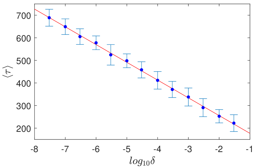
Figure 3: Scaling of the average chimera lifetime with perturbation. A fit of the data points gives the scaling between $\langle\tau\rangle$ and the magnitude of the dimension altering perturbation $\delta$ as $\langle\tau\rangle\sim-\log_{10}{\delta}$. Error bars represent standard deviations of the distributions. Parameter values are $N=256$, $A=0.995$, and $\alpha=\pi/2-0.05$.

For any transient phenomenon in nonlinear dynamics, a fundamental issue is the scaling law of the average transient lifetime with some system parameter variation, noise amplitude, or perturbation Grebogi et al. (1983); Lai and Tél (2011). A transient behavior will be physically equivalent to some attracting behavior if the transient lifetime diverges exponentially, as speculated in the case of turbulence Crutchfield and Kaneko (1988) or superpersistent chaotic transients Grebogi et al. (1985); Do and Lai (2003, 2004); D’Huys et al. (2016); Lohmann et al. (2017). Such scaling was also found for chimera states in networks of Boolean phase oscillators Rosin et al. (2014). Under a dimension-augmenting perturbation, how does the average chimera time scale with the perturbation strength? A representative result is shown in Fig. 3, where the average chimera time $\langle\tau\rangle$ (on a linear scale) is plotted against the perturbation magnitude $\delta$ (on a logarithmic scale). We have the scaling law: $\langle\tau\rangle\sim-\ln{\delta}$, the physical significance of which is that the transient lifetime is extraordinarily short, in contrast to many transient scaling laws in nonlinear dynamical systems Lai and Tél (2011). In fact, a reduction in the perturbation by many orders of magnitude results in only an incremental increase in the average chimera time. That is, an arbitrarily small perturbation that drives the oscillator dynamics away from 2D immediately destroys the long-transient chimera state.

Why does a chimera state collapse when the oscillator dynamics deviate away from 2D? The value of $R_{i}\chi_{i}$ is the key. In 3D, the dynamics of $\theta$ are governed by Eq. (8), where the only difference with the 2D model is the extra factor $\chi_{i}$. While it appears that, in 3D, the value of $R_{i}\chi_{i}$ may play a similar rule to that of $R_{i}$ in 2D, $R_{i}\chi_{i}$ is affected not only by the coherence of the oscillators about the $i$th oscillator, but also by the latitudinal angles of all the oscillators, especially $\gamma_{i}$. Typically, the value of $\Gamma_{i}$ is close to zero, but $\gamma_{i}$ can be away from zero. In 2D, since $R_{i}$ is a measure of coherence, its value for an oscillator in the incoherent region must be smaller than that in the coherent region. However, in 3D, incoherent oscillators can have larger $R_{i}\chi_{i}$ values than those of the coherent ones, because the former are less coherent and can diffuse away from the initial equator faster, resulting in larger values of $|\gamma_{i}|$. Similar to the role of large values of $R_{i}$ in 2D, large values of $R_{i}\chi_{i}$ in 3D will make the oscillators more coherent. Simulations have revealed (Sec. IV) that $R_{i}\chi_{i}$ can be large for many oscillators in the incoherent region, leading to the emergence of a new and wider coherent region within the incoherent region. After that, an increasing number of coherent regions form inside the remaining incoherent regions, making the whole system closer to being globally coherent.

The collapse of the 2D-like structure is then caused by the diffusion of oscillators in their $\gamma$ components. When the $\gamma_{i}$ values of some oscillators in the incoherent region are not close to zero, a new coherent region is formed. How far away from the initial equator the $\gamma_{i}$ values collectively are can be measured by the variance of $\gamma_{i}$, as shown in Fig. 1(c). We see that $\mbox{Var}(\gamma)$ tends to increase exponentially during the 2D-like chimera state, leading to the observed logarithmic dependence of the average lifetime on the perturbation strength. In particular, let $v_{max}$ be the threshold of $\mbox{Var}(\gamma)$ beyond which a new coherent region emerges and let $\langle t_{e}\rangle$ be the average time that the threshold is reached. We have

$$\delta\exp{(\kappa\langle t_{e}\rangle)}\sim v_{max}.$$

Since $\langle\tau\rangle\sim\langle t_{e}\rangle$, we get $\langle\tau\rangle\sim-\ln{\delta}$.

In the 2D system, the chimera states typically coexist with the complete synchronization state. This is the reason that we choose the values of $A$ and $\alpha$ to be close to one and $\pi/2$, respectively. In this parameter regime, the basin of the chimera states is relatively large, facilitating numerical observation of a chimera state with random initial conditions. It is insightful to compare the results with those for the case where the initial conditions are chosen from the basin of the complete synchronization state. In this case, we have that, after a short transient, the system approaches an asymptotically global synchronization state. The length of this transient is comparable to that of the transient before the emergence of the chimera states from initial condition in the chimera-state basin, which is about $t=120$ in Fig. 1(b). Upon a dimension-augmenting perturbation, the synchronous state of the system remains to be low-dimensional. That is, the system will not become 3D. We thus see that the situation with the chimera state is characteristically different: such a state becomes 3D but only for a short transient period of time before its collapse. This point can also be seen from Fig. 1(c) where, during the transient chimera phase, the system rapidly moves out of the equator, with an exponentially growing variance in the latitudinal angle $\gamma$.

III.2 Dependence of transient lifetime of chimera states on system size

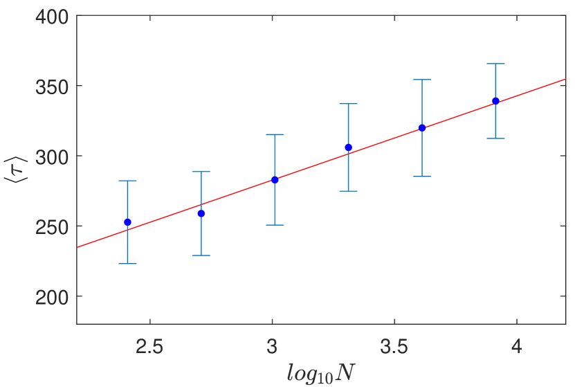
Figure 4: Average transient lifetime of chimera states versus system size in 3D. Shown are numerical results (dots) and linear fit (line). Error bars represent the standard deviations of the distributions. The system parameters are $T_{33}=-1$, $\theta_{d}=0.01$, $A=0.995$ and $\alpha=\pi/2-0.05$.

In 2D, the average lifetime of a chimera state grows exponentially with the system size, rendering infeasible numerical simulation Wolfrum and Omel’chenko (2011) for large systems. However, we find that, in higher dimensions, the average chimera time does not follow such a rule, as the mechanism of the collapse of the chimera state is quite different from that in 2D. Figure 4 shows that the average chimera time scales with the system size only logarithmically. The heuristic reason is that an increase in the number of oscillators weakens, on average, the influence of the perturbation applied to a single node on other nodes. Since the average chimera time scales with the magnitude of the perturbation only logarithmically, so should be its dependence on the system size.

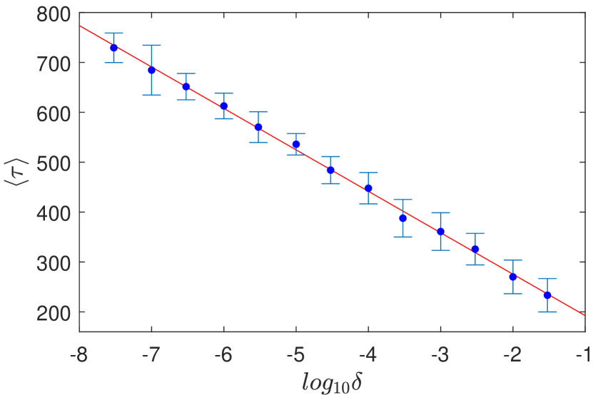
Figure 5: Scaling of the average chimera lifetime with perturbation for a larger system size. The system size is $N=1024$. The scaling law is essentially the same as that in Fig. 3 for $N=256$, with only about a $10\%$ increase in the average transient lifetime. Other parameter values are $T_{33}=-1$, $\theta_{d}=0.01$, $A=0.995$, and $\alpha=\pi/2-0.05$.

To assess the generality and reliability of the uncovered scaling law of the average chimera lifetime versus the dimension-augmenting perturbation, we have calculated the scaling law for different values of the system size $N$. An example is presented in Fig. 5, where the scaling law is obtained for $N=1024$. Comparing with the scaling law in Fig. 3 for $N=256$, we see that a four-fold increase in the system size does not change the logarithmic scaling law. In fact, the only noticeable change is a slight increase in the average lifetime (about $10\%$), due to the logarithmic nature of the scaling law. This provides further support for our finding of the fragility of the chimera state because a dramatic increase in the system size does not significantly prolong the transient. This should be contrasted to the case of chaotic transients in spatiotemporal dynamical systems, where the average transient lifetime typically increases extremely rapidly with the system size, often in a way that is faster than exponential growth Crutchfield and Kaneko (1988).

III.3 Dependence of average transient lifetime of chimera states on coupling parameters

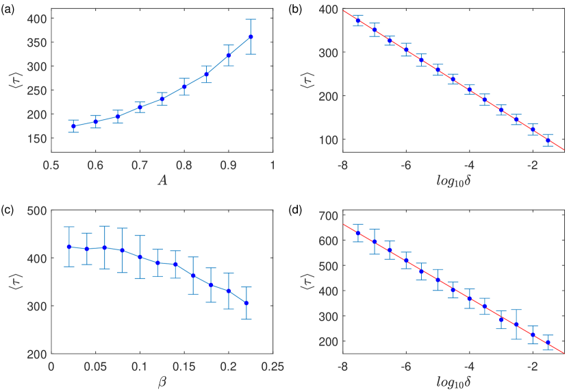
Figure 6: Average transient lifetime of chimera states and scaling law for different values of the coupling parameters $A$ and $\beta$ in 3D. (a) Average chimera lifetime versus $A$ for $T_{33}=-1$, $\theta_{d}=0.0001$, and $\beta=\pi/2-\alpha=0.05$. (b) A representative scaling law of the average chimera lifetime with perturbation for $A=0.7$, where other parameter values are the same as those in (a). (c) Average chimera lifetime versus $\beta$ for $T_{33}=-1$, $\theta_{d}=0.0001$, and $A=0.995$. (d) A representative scaling law for $\beta=0.15$. Other parameters are the same as those in (c). In all panels, the error bars represent the standard deviations of the probability distributions.

We study how the average transient lifetime of the chimera states depends on the coupling parameters $A$ and $\alpha$. For convenience, we introduce $\beta=\pi/2-\alpha$ to facilitate analysis of the situation where the value of $\alpha$ is close to $\pi/2$ and that of $A$ close to one so as to obtain a relatively large basin of the chimera states. In fact, as the values of $\beta$ and $A$ deviate from zero and one, respectively, the basin of the globally synchronized state will be enlarged, eventually making the basin of the chimera states vanish Abrams and Strogatz (2004).

Figure 6(a) shows that the average transient lifetime $\langle\tau\rangle$ of the chimera states increases with $A$, with a representative scaling law for $A=0.7$ shown in Fig. 6(b). Figure 6(c) shows the dependence of $\langle\tau\rangle$ on $\beta$, with the scaling law for $\beta=0.15$ shown in Fig. 6(d). In general, when the values of $A$ and $\beta$ move closer to the boundary beyond which chimera states no longer exist, the average transient lifetime decreases, due to the system’s transition into 3D as characterized by a faster growth of $Var(\gamma)$. In addition, not only will the proportion of the initial states that go directly to the complete synchronization state increase, but the final states after the collapse of a transient chimera state will also be different (see the last paragraph of Sec. IV for a further discussion of this phenomenon). Despite these behaviors, the logarithmic scaling law between the average transient time and perturbation remains invariant. These results, together with the results in Sec. III.2, attest to the remarkable robustness of the scaling law.

IV Mechanism of collapses of chimera states in high dimensions

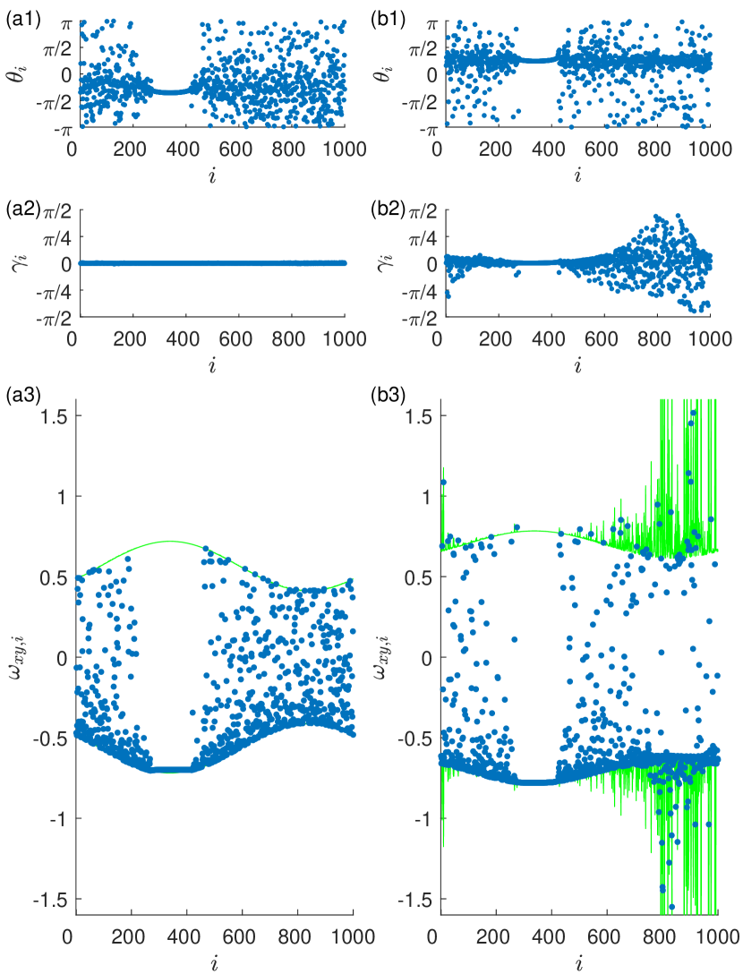
Figure 7: Snapshots of the 3D system. (a1, a2, a3) The first stage and (b1, b2, b3) the second stage as discussed in Sec. IV. (a1, b1) Snapshots of the longitudinal angles $\theta_{i}$ of the oscillators. In both stages, the system is in a chimera state in terms of component $\theta$. (a2, b2) Snapshots of the latitudinal angles $\gamma_{i}$ of the oscillators. In the first stage (a2), all $\gamma_{i}$ values are still close to zero, while in the second stage (b2) many oscillators close to the center of the incoherent region have $\gamma_{i}$ values away from zero. (a3, b3) Snapshots of the instantaneous angular velocity in the $(x,y)$-plane, $\omega_{xy,i}$ (blue dots), and $\pm R_{i}\chi_{i}$ (green traces) of all the oscillators. Equation (8) gives that $\omega_{xy,i}$ is bounded by $\pm R_{i}\chi_{i}$, which agrees with the simulation results. In the first stage (a3), the coherent region has the largest and locked values of $\omega_{xy,i}$, similar to the regular 2D chimera state, and the oscillators in the incoherent region cannot reach such a value of $\omega_{xy,i}$ since they are bounded by the smaller values of $R_{i}\chi_{i}$. However, in the second stage (b3), $\pm R\chi$ exhibits irregular spikes for a large number of oscillators close to the center of the incoherent region, so these oscillators can have similar value of $\omega_{xy,i}$ to that of locked $\omega_{xy}$ in the incoherent region, or even larger. This indicates that the local dynamics of these oscillators have already deviated significantly from the 2D-like structure.

The general picture of the collapse of the chimera state can be described in terms of five successive stages, as follows. In the first stage, a 2D-like chimera state is formed with the coexistence of a coherent and an incoherent region. In this stage, the components of the state vectors $\bm{\sigma}$ of all the oscillators in the third dimension, $\bm{\sigma}_{z}$, are small. In the spherical coordinates, all oscillators have their $\gamma$ values close to zero, so the corresponding $\chi$ values are all close to one. The incoherent region has a lower $R$ value due to its lack of coherence, so the corresponding value of $R\chi$ is also small, making the oscillators there less affected by the collective behavior. In our approach, the initial state is that all the oscillators have $\gamma_{i}=0$, except for one oscillator with a small perturbation $\gamma_{i}=\delta$. During the system evolution, the values of $\gamma_{i}$ in the incoherent region gradually diffuse due to interactions, while $\gamma$ in the coherent region remains at near zero values.

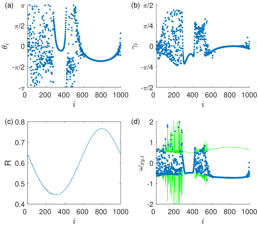
Figure 8: Snapshots of the same system in Fig. 7 in its third stage. (a) Snapshot of the longitudinal angles $\theta_{i}$ of the oscillators. A new coherent region is formed at roughly $600<i<800$, which is larger than the one in $300<i<400$ formed during the first stage shown in Figs. 7(a1,b1). The system is now in a multi-chimera state with several coherent and incoherent regions. (b) Snapshot of the latitudinal angles $\gamma_{i}$ of the oscillators. After the appearance of the new coherent region, the values of $\gamma_{i}$ of these oscillators in this region are close to zero, in contrast to the second stage. The angles $\gamma_{i}$ of the oscillators from the old coherent region deviate further away from zero than in the first and second stages, but they are still smaller than the angles of most oscillators in the incoherent regions. (c) Snapshot of the order parameter $R$. The peak is now at the center of the new coherent region. (d) Snapshots of the instantaneous angular velocity in the $(x,y)$-plane for all the oscillators: values of $\omega_{xy,i}$ (blue dots) and $\pm R_{i}\chi_{i}$ (green traces).

In the second stage, while the $\theta$ components of the oscillators are still in a chimera state, the $\gamma$ components of some oscillators are no longer close to zero and the average absolute value of $\gamma$ in the incoherent region becomes larger than that in the coherent region, as shown in Fig. 7(b2). Such high values of $\gamma$ make the value of $\chi$ high as well. As a result, in this stage many oscillators in the incoherent region have a larger average $R\chi$ value than those in the coherent region, as shown in Fig. 7(b3), a behavior that is opposite to that in the first stage. Moreover, from Eq. (8), we have that the instantaneous phase or angular velocity $d\theta/dt$ in the $(x,y)$-plane, $\omega_{xy}$, is bounded by $\pm R\chi$. A larger $R\chi$ value in the incoherent region can thus result in a larger absolute value of the phase velocity $|\omega_{xy}|$ than that in the coherent region, as shown in Fig. 7(b3). Note that, in the first stage, similar to the transient 2D chimera states with a long lifetime, the oscillators in the coherent region have the largest possible value of $|\omega_{xy}|$, as shown in Fig. 7(a3), making the oscillators in the incoherent region unable to synchronize with the coherent oscillators since the incoherent region does not have similarly large $R\chi$ values required for large values of $|\omega_{xy}|$. However, in the second stage, this is no longer the case: oscillators in the incoherent region can have $|\omega_{xy}|$ values larger than those in the coherent region, driving the system away from the 2D-like structure.

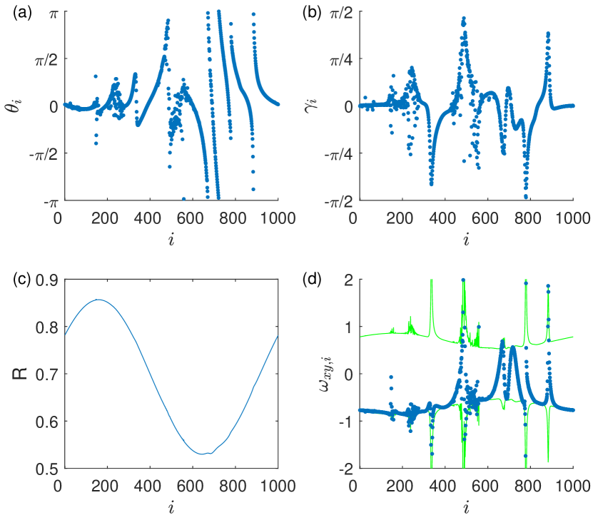
Figure 9: Snapshots of the same system in Figs. 7 and 8 in the fourth stage. (a,b) Snapshots of $\theta_{i}$ and $\gamma_{i}$. (c) Snapshot of the order parameter $R$. The peak is now at a new location away from its location in the third stage. (d) Snapshots of the instantaneous angular velocity in the $(x,y)$-plane of all the oscillators: $\omega_{xy,i}$ (blue dots) and $\pm R_{i}\chi_{i}$ (green traces). The system is now more fragmental than in the third stage: the extensive coherent region from the third stage has now broken into several coherent and incoherent regions.

As a consequence of large values of $R\chi$, in the third stage, a new and even wider coherent region emerges within the incoherent region, placing the whole system in a transient multi-chimera state with two coherent regions: one is formed at the beginning of the first stage and the other newly appeared one emerging inside the incoherent region, as shown in Fig. 8. In the third stage, the region used to be the most incoherent becomes now the most coherent with the largest value of $R$ and a larger size than the original coherent region. The $R$ value of the original coherent region is now close to its minimum value. These observations suggest a negative feedback mechanism. In particular, incoherence in the first stage results in small $R_{i}$ values and thus small $R_{i}\chi_{i}$ values as well, making $\gamma_{i}$ deviate away from zero, which in turn results in a high value of $R_{i}\chi_{i}$ that leads to incoherence. As a result, coherence in the system has been undermined, leading to near zero average value of $\gamma_{i}$, as the oscillators have evenly distributed positive and negative $\gamma_{i}$ values. This leads to a small average value of $R_{i}\chi_{i}$, making it difficult for the oscillators to remain coherent. While this mechanism does not turn coherence into incoherence as effectively as a large value of $R_{i}\chi_{i}$ turns incoherence into coherence, a fraction of the oscillators still have a large average $\gamma$ value. The difference drives the whole system towards global coherence.

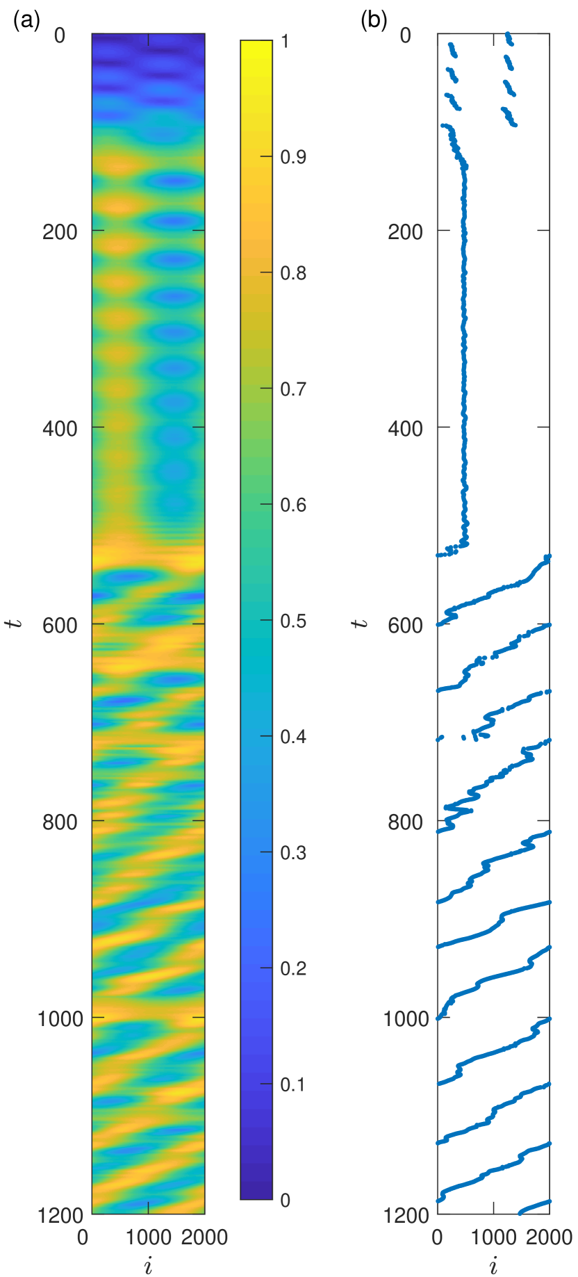
Figure 10: Spatial distribution of the order parameter of the oscillators. (a) Value of the order parameter $R$ of all the oscillators. (b) The location of the oscillator with the largest value of $R$ among all the oscillators versus time, which is constantly traveling across the system after the collapse of the 2D-like chimera state at $t=540.9$.

In the fourth stage, a process similar to that in the third stage occurs, where large coherent and incoherent regions break into smaller subregions of coherence and incoherence. An example is shown in Fig. 9. The system becomes fragmental without any recognizable pattern. There are two major sources of randomness. Firstly, oscillators in the same coherent region are phase-locked in the $\theta$ component, but the locked phase velocities are different from region to region. Because these coherent regions have different average values of $R$ and $R\chi$. Secondly, the positions of the newly formed regions are sensitive to the random initial condition, rendering random sizes of the regions.

In the final stage, the system is close to a globally coherent state, but can never actually reach it. The global state is dynamical, with the emergence and disappearance of many fragmental coherent regions driven by the negative feedback mechanism discussed above. Globally, $g_{0}$ reaches a relatively stable value with fluctuations, as shown in Fig. 1(b). Several snapshots of this stage are shown in Fig. 2(b1-b4).

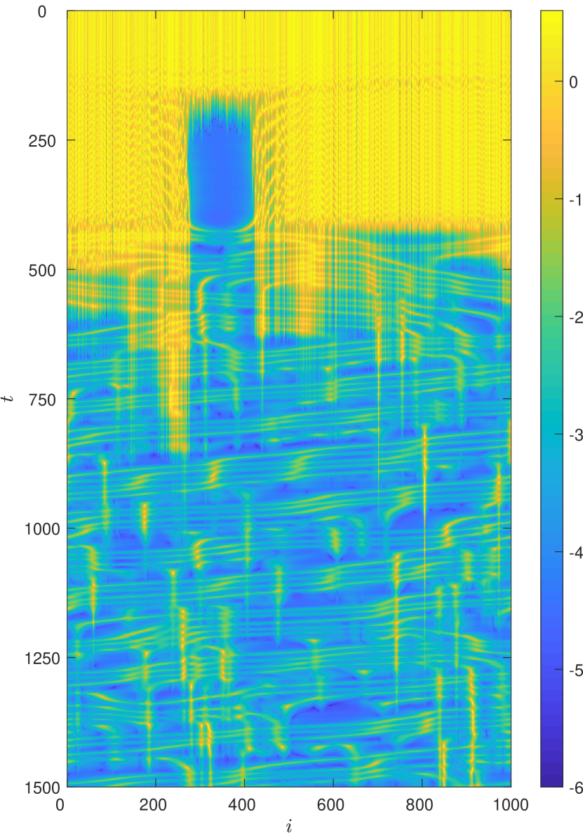
Figure 11: Temporal evolution of $\log_{10}{D_{i}}$. The regions with $\log_{10}{D_{i}}<-2$ are classified as coherent regions. Other regions are classified as incoherent regions. Note that there is coexistence of one coherent and another incoherent regions in the system in the time interval $150\lesssim t\lesssim 400$, indicating a transient chimera state.

Figures 10 and 11 present additional evidence to support our understanding of the fragility of the chimera state. In particular, Fig. 10(a) shows the location of the oscillators with the largest value of the order parameter $R$ among all other oscillators at a time instant. Because of the choice of a non-local/non-global coupling function $G(i-j)$ and the order parameter defined as $\bm{\rho}_{i}=N^{-1}\sum_{j=1}^{N}G(i-j)\bm{\sigma}_{j}$, the position at which $R$ reaches the maximum value gives information about the center of the non-local/non-global coherent region. Prior to the collapse of the 2D-like chimera state, this position remains at the center of the coherent region. However, after the collapse, the position constantly rotates among different oscillators. As shown in Fig. 11, the coherent regions with a low value of $\log_{10}{D_{i}}$, denoted by the blue color, have short lifetime in the stages after the collapse of the chimera state. During those stages, the values of $\log_{10}{D_{i}}$ of different regions in the system oscillate. This also agrees with our understanding that a high value of $\gamma$ would decrease soon due to the negative feedback mechanism.

The results studied so far are for the case where the values of the coupling parameters $A$ and $\alpha$ are away from the boundary of the basin of the chimera states. As this boundary is approached, another type of final states after the collapse of the transient chimera states appears, which is the global synchronization state. The fraction of the initial states leading to this synchronous state increases toward one. (Here we exclude the cases where no chimera state ever appears and the system directly goes to global synchronization, and focus on the cases where there was a chimera state.) The origin of this alternative final state can be understood as follows: near the basin boundary, the relative size of the coherent region associated with the chimera state becomes larger. As explained, in the third stage a second and even larger coherent region will emerge in the middle of the incoherent region. Since the first coherent region has already become relatively large (e.g., about half the size of the whole system), the final state contains a large coherent region as in the third stage.

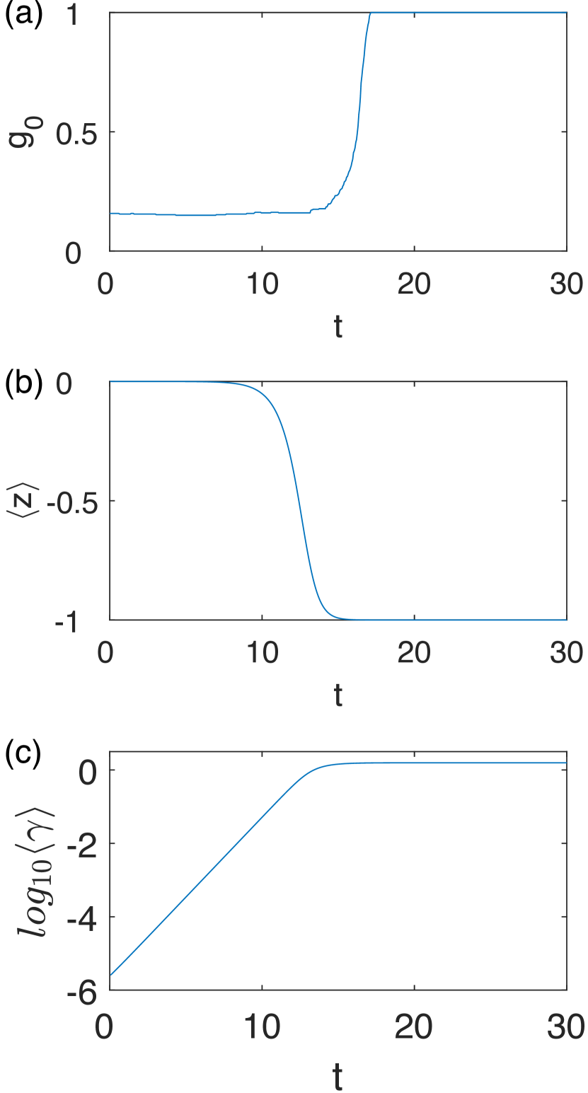
Figure 12: Transient chimera state in 3D systems with $T_{33}=+1$. (a) Time evolution of $g_{0}$ with initial perturbation $\delta=10^{-3}$. The transient time before the system collapses into a global synchronized state (where $g_{0}=1$) is one order of magnitude shorter than that for the case of $T_{33}=-1$ for the same value of $\delta$ (c.f., Fig. 3). (b) Time evolution of the average $z$ component (in Cartesian coordinates) of all the oscillators, which converges rapidly to $-1$, indicating that all phase vectors $\sigma_{i}$ are concentrating at the “south pole” of the unit sphere $S^{2}$ after a short transient. (c) Logarithm of the time evolution of the average latitudinal angle of all oscillators. The approximately linear growth of the logarithm indicates an exponential growth of the average latitudinal angle during the transient. System parameter values are $N=400$, $\theta_{d}=0.001$, $\alpha=\pi/2-0.05$, and $A=0.995$.

V 3D systems with $T_{33}=+1$ and 4D systems

We see from Sec. II that there is another possible case in 3D where $T_{33}=+1$. A difficulty is that, for $T_{33}=+1$, any 2D structure is physically or computationally not observable because an infinitesimal perturbation (e.g., on the order of the computer round off error) is sufficient to destroy the 2D structure even before the emergency of any transient chimera state. To overcome this difficulty, we first generate chimera states in a purely 2D system, and then perturb these 2D chimera configurations and use them as the initial states for the $T_{33}=+1$ systems. The systems are then initially in chimera states. With this initial chimera state, the oscillators still quickly synchronize to the fixed points of the transformation $\bm{{\rm T}}$: $(0,0,\pm 1)$ (in Cartesian coordinates), as shown in Fig. 12. Since the longitudinal angles at the fixed points are zero, the phase lag plays no role in the dynamics. In the high-dimensional Kuramoto model with no phase lag, all the oscillators have the same natural frequency, making the synchronized state stable Chandra et al. (2019a).

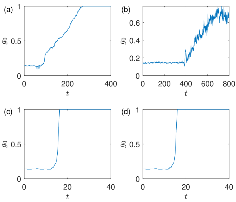
Figure 13: Transient chimera states in 4D. Shown is the time evolution of $g_{0}$ in four different types of 4D systems: (a) $k=2$ and $m=0$, (b) $k=1$ and $m=2$, (c) $k=1$ and $m=1$, (d) $k=1$ and $m=0$. In all four cases, the double rotation matrix $\bm{{\rm T}}$ has $\alpha_{1}=\pi/2-0.05$ and $\alpha_{2}=\pi/2-0.06$. All four systems start from the same 2D chimera state as the initial conditions, with a perturbation of $\phi_{2,d}=\phi_{3,d}=0.001$ in the second and third angular coordinates in the 4D spherical coordinate system. The values of other system parameters are $N=256$ and $A=0.995$. In all cases, the initial 2D chimera state can last only for a short time before being destroyed.

Insights into this behavior can be gained by analyzing the linearized approximation of Eq. (3), as the values of $\gamma_{i}$ and $\Gamma_{i}$ are typically small before the collapse:

$$\frac{d\gamma_{i}}{dt}=R_{i}\times\left[-cos\left(\theta_{i}-\Theta_{i}+\alpha\right)\gamma_{i}+\Gamma_{i}\right],$$ (11)

where $R_{i}$ is positive. The quantity $\left(\theta_{i}-\Theta_{i}+\alpha\right)$ exhibits rapid oscillations in the interval $[-\pi,\pi)$ without an apparent pattern, so the quantity $-\cos\left(\theta_{i}-\Theta_{i}+\alpha\right)$ oscillates within the interval $[-1,1]$ approximately randomly. The sign of the factor $-R_{i}\times\cos\left(\theta_{i}-\Theta_{i}+\alpha\right)\gamma_{i}$ thus changes rapidly, while the sign of $R_{i}$ remains positive. As a result, the $R_{i}\Gamma_{i}$ component plays a major role in the dynamics, making the absolute value of $\gamma_{i}$ increase exponentially. This agrees with the simulation result, as shown in Fig. 12(c), where we observe that the average $\gamma$ value indeed grows exponentially in time.

We see from Sec. II that four different forms of the matrix $\bm{{\rm T}}$ can arise in 4D. We encounter the similar difficulty in all these four forms as in the $T_{33}=+1$ case in 3D: an infinitesimal perturbation on the order of the computer round off error is sufficient to destroy the 2D structure before the emergency of any transient chimera state. Thus in all the four different cases we let the system begin with 2D chimera states as for the $T_{33}=+1$ case in 3D. Figure 13 shows the representative results on the dynamical evolution of a 4D system from the initial chimera state. In all cases, the chimera state can last for a relatively short time only, indicating that, in 4D, chimera states (even of an appreciable transient lifetime) are unlikely to occur.

VI Discussion

To summarize, our finding of an extreme type of fragility of chimera states against dimension-augmenting perturbations beyond 2D, quantitatively characterized by a logarithmic scaling law, has implications with respect to observability. We also note that, in 2D, when the number $N$ of oscillators is finite, chimera states are long transients Wolfrum and Omel’chenko (2011) and their average lifetime increases exponentially with $N$. However, in our case, the transient lifetime increases logarithmically with $N$. Indeed, we have never observed long transients in higher dimensions, even when there are thousands of oscillators in the system.

Besides the characteristically distinct scaling laws of the average transient lifetime, there are other differences between the 2D and dimension-augmenting transient chimera states. In 2D, the distribution of the transient lifetime from random initial conditions is exponential. However, in our model, the distribution is approximately Gaussian, with a small standard deviation (less than 10% of the mean value, as shown in Figs. 3-6). This means that the transient lifetime is much more closely clustered near the mean value in our model than in the 2D case. In general, when the system is in a particular transient chimera state, it is difficult to predict when it will collapse into 2D, as the transient states preceding the collapse exhibit a similar pattern. However, in our model, we can use a variable such as the spatial variance of $\gamma$ [as in Fig. 1(c)] as an indicator to predict any possible collapse, as it tends to increase monotonously towards a threshold value. In 2D, the transient chimera states are reported to belong to type-II supertransients Wolfrum and Omel’chenko (2011) by the criterion in Ref. Crutchfield and Kaneko (1988), which have the following features: an exponential scaling law of the transient lifetime with respect to system size, the exponential distribution of the transient lifetime, and stationarity of the patterns. Transient chimera states in 2D have all these features, but none can be found in our 3D or 4D systems. This further indicates the characteristically different nature of the transient chimera states in dimension-augmented systems from those in 2D.

There were previous studies on transient chimera states with respect to changes in the inertia of the oscillators Olmi (2015); Laing (2019) where, in the model studied, a change in the inertia from a non-zero value to zero can abruptly alter the dynamical behavior of the system, making the chimera state more unstable. Our results demonstrate that a dimension-augmenting perturbation can also make the chimera state extremely unstable in the sense of the scaling law uncovered. However, our model is the first-order Kuramoto system with 3D phase oscillators and the model previously studied Olmi (2015); Laing (2019) is a second-order phase Kuramoto system with inertia. The system settings are thus quite different. Further, the results are quite different as well: our main result is the logarithmic scaling law of the average transient lifetime of the chimera state with respect to both the perturbation magnitude, which holds regardless of the system size. In the previous studies Olmi (2015); Laing (2019), no such scaling law was reported; instead, the scaling law of the intermittent chaotic chimeras lifetime therein was found to be algebraic.

The chimera states can be long lasting when the dynamics of the oscillators are strictly equivalent to those of 2D rotors. Any deviation in the rotation dynamics from 2D will make a chimera state transient, with an extraordinarily short lifetime in the sense of the scaling law uncovered. However, there are situations where chimera states with a short lifetime may still be physically meaningful and observable. For example, for a highly dynamic system whose state changes constantly with time, the intrinsic time scale is short. In this case, if the time scale is shorter than the average transient lifetime of the chimera states, they are still physically meaningful and observable.

A recent analysis of synchronization in high-dimensional Kuramoto models Chandra et al. (2019b) revealed the existence of an invariant manifold of state distribution in the thermodynamic limit $N\to\infty$, which is an extension of the previous work on the 2D Kuramoto model Ott and Antonsen (2008, 2009). This manifold is attracting in 2D Ott and Antonsen (2009) and is likely to be attracting in high dimensions as well. However, chimera states, even in 2D, do not live on the invariant manifold. In higher dimensions, the manifold is circularly symmetric about some axis and the density of the distribution decreases monotonously from one axis pole to another. If the manifold is attracting, a 2D chimera state would naturally collapse and approach the attracting manifold, even when the system size is large. In higher dimensions, the picture is less clear as to whether the manifold is attracting. Identifying the existence of some invariant manifold and determining its stability may provide an avenue to study collective dynamics in high-dimensional Kuramoto models.

We remark that global synchronization in the high-dimensional Kuramoto model has been treated Chandra et al. (2019a, b), where it was shown that synchronization is stable under small perturbations. Global and cluster synchronization states in the high-dimensional Kuramoto model and their stability are different from our problem of the effect of dimension-augmenting perturbations on chimera states. In our setting, to generate chimera states, there are phase lags among the oscillators but their natural frequencies are identical. The common, natural rotation of the oscillators can then be excluded from consideration through the reference frame rotating at the same frequency. This should be contrasted to the setting of global and cluster synchronization, where the natural frequencies of the oscillators are different and follow a certain distribution and this heterogeneity plays an important role in synchronization. For example, for even dimensional models the criteria of whether an oscillator belongs to the entrained population or the drifting population depends on the value of the frequency of the natural rotation of the oscillator.

Appendix A Measure for detecting transient chimera states and determination of their lifetime

For all the simulations we use the fourth-order Runge-Kutta method to integrate the coupled networked system with time step $dt=0.005$. In particular, we integrate the system with the order parameter defined as $\bm{\rho}_{i}=N^{-1}\sum_{j=1}^{N}G(i-j)\bm{\sigma}_{j}$. When the local order parameter of oscillator $i$ includes a small self-coupling component, the average lifetime of the chimera state is longer than that in systems without such self-coupling. However, inclusion of the self-coupling term has little effect on the scaling law between the average chimera time and the magnitude of the perturbation.

To ascertain the existence of a transient chimera state, we use the measure $g_{0}$ introduced in Ref. Kemeth et al. (2016), which is the relative size of the coherent region. To calculate $g_{0}$, another quantity $D_{i}$ is needed, which is the spatial Laplacian of $\bm{\sigma}$ at oscillator $i$ that characterizes the instant local degree of distortion of its dynamical variables:

$$D_{i} = [\left(x_{i+1}-2x_{i}+x_{i-1}\right)^{2}+\left(y_{i+1}-2y_{i}+y_{i-1}\right)^{2}$$ (12)

$$+ \left(z_{i+1}-z_{i}+z_{i-1}\right)^{2}]^{1/2},$$

where $x_{i}$, $y_{i}$ and $z_{i}$ are the Cartesian coordinates of the 3D state vector of oscillator $i$. If the value of $D_{i}$ is smaller than a certain threshold, oscillator $i$ is regarded as being within the coherent region; otherwise it is in an incoherent region. The value of $g_{0}$ at time $t$ is calculated by counting the number of oscillators with $D_{i}$ smaller than the threshold at this time, normalized by the total number $N$ of oscillators. In our study, we choose the threshold value of $D_{i}$ to be $0.04$, which is approximately one hundredth of the upper bound of $D_{i}$.

When the system exhibits a chimera state, coherent and incoherent regions coexist, so we have $0\leq g_{0}\leq 1$. Furthermore, $g_{0}$ will be plateaued at a certain value with small fluctuations about it Kemeth et al. (2016). This provides a convenient and effective way to detect the transient chimera state. Especially, when the value of $g_{0}$ reaches a relatively flat plateau, the chimera state begins. The transient chimera state ends when the value of $g_{0}$ begins to deviate from the plateaued value.

Our algorithm to find the exact starting time and ending time of a transient chimera state can be described, as follows.

1. Roughly choose a interval of the value of $g_{0}$ which include the values of $g_{0}$ in the transient chimera states. With a certain set of system parameters, the value of $g_{0}$ in the chimera states are roughly similar. This interval does not need to be very accurate.

2. Determine the time interval in which the value of $g_{0}$ is in the interval chosen in step 1.

3. Calculate the average $g_{0}$ value in this time interval.

4. Measure the starting time of chimera state as the first time $g_{0}$ reaches the average value minus a small threshold value. We choose the threshold to be $0.05$ in this paper.

5. Determine the ending time of the chimera state as the last time when the value of $g_{0}$ is smaller than the same average adding the threshold value, before the value of $g_{0}$ ever grows beyond the average plus two times the threshold value.

6. The starting and ending time so determined can be inaccurate because of the chosen initial time interval from step 2. To increase the accuracy, we set the period between the starting and ending time as the new initial time interval.

7. Repeat steps 3-6 for 5 times to make the results converge.

We determine the ending point this way because $g_{0}$ sometimes fluctuates in a chimera state. The fluctuations arise even in purely 2D chimera states and can be relatively large. We choose some appropriate threshold value (e.g., $0.05$) to distinguish the cases when the system is in a chimera state and when it has left the state.

References

- Umberger et al. (1989) D. K. Umberger, C. Grebogi, E. Ott, and B. Afeyan, “Spatiotemporal dynamics in a dispersively coupled chain of nonlinear oscillators,” Phys. Rev. A 39, 4835 (1989).
- Kuramoto and Battogtokh (2002) Y. Kuramoto and D. Battogtokh, “Coexistence of coherence and incoherence in nonlocally coupled phase oscillators,” Nonlin. Phenom. Complex Syst. 5, 380 (2002).
- Abrams and Strogatz (2004) D. M. Abrams and S. H. Strogatz, “Chimera states for coupled oscillators,” Phys. Rev. Lett. 93, 174102 (2004).
- Shima and Kuramoto (2004) S.-I. Shima and Y. Kuramoto, “Rotating spiral waves with phase-randomized core in nonlocally coupled oscillators,” Phys. Rev. E 69, 036213 (2004).
- Abrams and Strogatz (2006) D. M. Abrams and S. H. Strogatz, “Chimera states in a ring of nonlocally coupled oscillators,” Int. J. Bif. Chaos 16, 21 (2006).
- Abrams et al. (2008) D. M. Abrams, R. Mirollo, S. H. Strogatz, and D. A. Wiley, “Solvable model for chimera states of coupled oscillators,” Phys. Rev. Lett. 101, 084103 (2008).
- Sethia et al. (2008) G. C. Sethia, A. Sen, and F. M. Atay, “Clustered chimera states in delay-coupled oscillator systems,” Phys. Rev. Lett. 100, 144102 (2008).
- Laing (2009) C. R. Laing, “Chimera states in heterogeneous networks,” Chaos 19, 013113 (2009).
- Sheeba et al. (2009) J. H. Sheeba, V. K. Chandrasekar, and M. Lakshmanan, “Globally clustered chimera states in delay-coupled populations,” Phys. Rev. E 79, 055203 (2009).
- Martens (2010) E. A. Martens, “Chimeras in a network of three oscillator populations with varying network topology,” Chaos 20, 043122 (2010).
- Martens et al. (2010) E. A. Martens, C. R. Laing, and S. H. Strogatz, “Solvable model of spiral wave chimeras,” Phys. Rev. Lett. 104, 044101 (2010).
- Omel’chenko et al. (2010) O. E. Omel’chenko, M. Wolfrum, and Y. L. Maistrenko, “Chimera states as chaotic spatiotemporal patterns,” Phys. Rev. E 81, 065201 (2010).
- Wolfrum and Omel’chenko (2011) M. Wolfrum and O. E. Omel’chenko, “Chimera states are chaotic transients,” Phys. Rev. E 84, 015201 (2011).
- Wolfrum et al. (2011) M. Wolfrum, O. E. Omel’chenko, S. Yanchuk, and Y. L. Maistrenko, “Spectral properties of chimera states,” Chaos 21, 013112 (2011).
- Omelchenko et al. (2011) I. Omelchenko, Y. Maistrenko, P. Hövel, and E. Schöll, “Loss of coherence in dynamical networks: Spatial chaos and chimera states,” Phys. Rev. Lett. 106, 234102 (2011).
- Omel’chenko et al. (2012) O. E. Omel’chenko, M. Wolfrum, S. Yanchuk, Y. L. Maistrenko, and O. Sudakov, “Stationary patterns of coherence and incoherence in two-dimensional arrays of non-locally-coupled phase oscillators,” Phys. Rev. E 85, 036210 (2012).
- Zhu et al. (2012) Y. Zhu, Y. Li, M. Zhang, and J. Yang, “The oscillating two-cluster chimera state in non-locally coupled phase oscillators,” EPL (Europhys. Lett.) 97, 10009 (2012).
- Laing et al. (2012) C. R. Laing, K. Rajendran, and I. G. Kevrekidis, “Chimeras in random non-complete networks of phase oscillators,” Chaos 22, 013132 (2012).
- Tinsley et al. (2012) M. R. Tinsley, S. Nkomo, and K. Showalter, “Chimera and phase-cluster states in populations of coupled chemical oscillators,” Nat. Phys. 8, 662 (2012).
- Hagerstrom et al. (2012) A. M. Hagerstrom, T. E. Murphy, R. Roy, P. Hövel, I. Omelchenko, and E. Schöll, “Experimental observation of chimeras in coupled-map lattices,” Nat. Phys. 8, 658 (2012).
- Omelchenko et al. (2013) I. Omelchenko, E. Omel chenko, P. Hövel, and E. Schöll, “When nonlocal coupling between oscillators becomes stronger: Patched synchrony or multichimera states,” Phys. Rev. Lett. 110, 224101 (2013).
- Ujjwal and Ramaswamy (2013) S. R. Ujjwal and R. Ramaswamy, “Chimeras with multiple coherent regions,” Phys. Rev. E 88, 032902 (2013).
- Zhu et al. (2013) Y. Zhu, Z. Zheng, and J. Yang, “Reversed two-cluster chimera state in non-locally coupled oscillators with heterogeneous phase lags,” EPL (Europhys. Lett.) 103, 10007 (2013).
- Yao et al. (2013) N. Yao, Z.-G. Huang, Y.-C. Lai, and Z.-G. Zheng, “Robustness of chimera states in complex dynamical systems,” Sci. Rep. 3, 3522 (2013).
- Nkomo et al. (2013) S. Nkomo, M. R. Tinsley, and K. Showalter, “Chimera states in populations of nonlocally coupled chemical oscillators,” Phys. Rev. Lett. 110, 244102 (2013).
- Martens et al. (2013) E. A. Martens, S. Thutupalli, A. Fourrière, and O. Hallatschek, “Chimera states in mechanical oscillator networks,” Proc. Nat. Acad. Sci. (USA) 110, 10563 (2013).
- Larger et al. (2013) L. Larger, B. Penkovsky, and Y. Maistrenko, “Virtual chimera states for delayed-feedback systems,” Phys. Rev. Lett. 111, 054103 (2013).
- Panaggio and Abrams (2013) M. J. Panaggio and D. M. Abrams, “Chimera states on a flat torus,” Phys. Rev. Lett. 110, 094102 (2013).
- Gu et al. (2013) C. Gu, G. St-Yves, and J. Davidsen, “Spiral wave chimeras in complex oscillatory and chaotic systems,” Phys. Rev. Lett. 111, 134101 (2013).
- Sieber et al. (2014) J. Sieber, O. E. Omel’chenko, and M. Wolfrum, “Controlling unstable chaos: Stabilizing chimera states by feedback,” Phys. Rev. Lett. 112, 054102 (2014).
- Schmidt et al. (2014) L. Schmidt, K. Schönleber, K. Krischer, and V. García-Morales, “Coexistence of synchrony and incoherence in oscillatory media under nonlinear global coupling,” Chaos 24, 013102 (2014).
- Zhu et al. (2014) Y. Zhu, Z. Zheng, and J. Yang, “Chimera states on complex networks,” Phys. Rev. E 89, 022914 (2014).
- Omel’chenko (2013) O. E. Omel’chenko, “Coherence-incoherence patterns in a ring of non-locally coupled phase oscillators,” Nonlinearity 26, 2469 (2013).
- Omel’chenko et al. (2008) O. E. Omel’chenko, Y. L. Maistrenko, and P. A. Tass, “Chimera states: The natural link between coherence and incoherence,” Phys. Rev. Lett. 100, 044105 (2008).
- Xie et al. (2014) J. Xie, E. Knobloch, and H.-C. Kao, “Multicluster and traveling chimera states in nonlocal phase-coupled oscillators,” Phys. Rev. E 90, 022919 (2014).
- Yao et al. (2015) N. Yao, Z.-G. Huang, C. Grebogi, and Y.-C. Lai, “Emergence of multicluster chimera states,” Sci. Rep. 5, 12988 (2015).
- Maistrenko et al. (2015) Y. Maistrenko, O.Sudakov, O. Osiv, and V. Maistrenko, “Chimera states in three dimensions,” New J. Phys. 17, 073037 (2015).
- Panaggio and Abrams (2015a) M. J. Panaggio and D. M. Abrams, “Chimera states on the surface of a sphere,” Phys. Rev. E. 91, 022909 (2015a).
- Panaggio and Abrams (2015b) M. J. Panaggio and D. M. Abrams, “Chimera states: Coexistence of coherence and incoherence in networks of coupled oscillators,” Nonlinearity 28, R67 (2015b).
- Martens and Bick (2015) E. A. Martens and C. Bick, “Controlling chimeras,” New J. Phys. 17, 033030 (2015).
- Omelchenko et al. (2015a) I. Omelchenko, A. Zakharova, P. Hövel, J. Siebert, and E. Schöll, “Nonlinearity of local dynamics promotes multi-chimeras,” Chaos 25, 083104 (2015a).
- Böhm et al. (2015) F. Böhm, A. Zakharova, E. Schöll, and K. Lüdge, “Amplitude-phase coupling drives chimera states in globally coupled laser networks,” Phys. Rev. E 91, 040901 (2015).
- Nkomo et al. (2016) S. Nkomo, M. R. Tinsley, and K. Showalter, “Chimera and chimera-like states in populations of nonlocally coupled homogeneous and heterogeneous chemical oscillators,” Chaos 26, 094826 (2016).
- Viennot and Aubourg (2016) D. Viennot and L. Aubourg, “Quantum chimera states,” Phys. Lett. A 380, 678 (2016).
- Hart et al. (2016) J. D. Hart, K. Bansal, T. E. Murphy, and R. Roy, “Experimental observation of chimera and cluster states in a minimal globally coupled network,” Chaos 26, 094801 (2016).
- Gambuzza and Frasca (2016) L. V. Gambuzza and M. Frasca, “Pinning control of chimera states,” Phys. Rev. E 94, 022306 (2016).
- Semenov et al. (2016) V. Semenov, A. Zakharova, Y. Maistrenko, and E. Schöll, “Deterministic and stochastic control of chimera states in delayed feedback oscillator,” AIP Conf. Proc. 1738, 210013 (2016).
- Kemeth et al. (2016) F. P. Kemeth, S. W. Haugland, L. Schmidt, I. G. Kevrekidis, and K. Krischer, “A classification scheme for chimera states,” Chaos 26, 094815 (2016).
- Ulonskaa et al. (2016) S. Ulonskaa, I. Omelchenko, A. Zakharova, and E. Schöll, “Chimera states in networks of van der Pol oscillators with hierarchical connectivities,” Chaos 26, 094825 (2016).
- Andrzejak et al. (2017) R. G. Andrzejak, G. Ruzzene, and I. Malvestio, “Generalized synchronization between chimera states,” Chaos 27, 053114 (2017).
- Bera et al. (2017) B. K. Bera, S. Majhi, D. Ghosh, and M. Perc, “Chimera states: Effects of different coupling topologies,” EPL (Europhys. Lett.) 118, 10001 (2017).
- Rakshit et al. (2017) S. Rakshit, B. K. Bera, M. Perc, and D. Ghosh, “Basin stability for chimera states,” Sci. Rep. 7, 2412 (2017).
- Semenova et al. (2017) N. I. Semenova, G. I. Strelkova, V. S. Anishchenko, and A. Zakharova, “Temporal intermittency and the lifetime of chimera states in ensembles of nonlocally coupled chaotic oscillators,” Chaos 27, 061102 (2017).
- Malchow et al. (2018) A.-K. Malchow, I. Omelchenko, E. Schöll, and P. Hövel, “Robustness of chimera states in nonlocally coupled networks of nonidentical logistic maps,” Phys. Rev. E 98, 012217 (2018).
- Botha and Kolahchi (2018) A. E. Botha and M. R. Kolahchi, “Analysis of chimera states as drive-response systems,” Sci. Rep. 8, 1830 (2018).
- Omelchenko et al. (2018) I. Omelchenko, O. E. Omel’chenko, A. Zakharova, and E. Schöll, “Optimal design of tweezer control for chimera states,” Phys. Rev. E 97, 012216 (2018).
- Xu et al. (2018) H.-Y. Xu, G.-L. Wang, L. Huang, and Y.-C. Lai, “Chaos in Dirac electron optics: Emergence of a relativistic quantum chimera,” Phys. Rev. Lett. 120, 124101 (2018).
- Yao et al. (2019) N. Yao, Z.-G. Huang, H.-P. Ren, C. Grebogi, and Y.-C. Lai, “Self-adaptation of chimera states,” Phys. Rev. E 99, 010201 (2019).
- Omelchenko et al. (2015b) I. Omelchenko, A. Provata, J. Hizanidis, E. Schöll, and P. Hövel, “Robustness of chimera states for coupled FitzHugh-Nagumo oscillators,” Phys. Rev. E 91, 022917 (2015b).
- Loos et al. (2016) S. A. M. Loos, J. C. Claussen, E. Schöll, and A. Zakharova, “Chimera patterns under the impact of noise,” Phys. Rev. E 93, 012209 (2016).
- Olfati-Saber (2006) R. Olfati-Saber, “Swarms on sphere: A programmable swarm with synchronous behaviors like oscillator networks,” in Proceedings of the 45th IEEE Conference on Decision and Control (IEEE, 2006) pp. 5060–5066.
- Lohe (2009) M. Lohe, “Non-Abelian Kuramoto models and synchronization,” J. Phys. A Math. Theo. 42, 395101 (2009).
- Chandra et al. (2019a) S. Chandra, M. Girvan, and E. Ott, “Continuous versus discontinuous transitions in the D-dimensional generalized Kuramoto model: Odd D is different,” Phys. Rev. X 9, 011002 (2019a).
- Chandra et al. (2019b) S. Chandra, M. Girvan, and E. Ott, “Complexity reduction ansatz for systems of interacting orientable agents: Beyond the Kuramoto model,” Chaos 29, 053107 (2019b).
- Grebogi et al. (1983) C. Grebogi, E. Ott, and J. A. Yorke, “Crises, sudden changes in chaotic attractors and chaotic transients,” Physica D 7, 181 (1983).
- Lai and Tél (2011) Y.-C. Lai and T. Tél, Transient Chaos: Complex Dynamics on Finite Time Scales, Vol. 173 (Springer, New York, 2011).
- Crutchfield and Kaneko (1988) J. R. Crutchfield and K. Kaneko, “Are attractors relevant to turbulence?” Phys. Rev. Lett. 60, 2715 (1988).
- Grebogi et al. (1985) C. Grebogi, E. Ott, and J. Yorke, “Super persistent chaotic transients,” Ergod. Theor. Dyn. Syst. 5, 341 (1985).
- Do and Lai (2003) Y. Do and Y.-C. Lai, “Superpersistent chaotic transients in physical space: advective dynamics of inertial particles in open chaotic flows under noise,” Phys. Rev. Lett. 91, 224101 (2003).
- Do and Lai (2004) Y. Do and Y.-C. Lai, “Extraordinarily superpersistent chaotic transients,” EPL (Europhys. Lett.) 67, 914 (2004).
- D’Huys et al. (2016) O. D’Huys, J. Lohmann, N. D. Haynes, and D. J. Gauthier, “Super-transient scaling in time-delay autonomous boolean network motifs,” Chaos 26, 094810 (2016).
- Lohmann et al. (2017) J. Lohmann, O. D’Huys, N. D. Haynes, E. Schöll, and D. J. Gauthier, “Transient dynamics and their control in time-delay autonomous boolean ring networks,” Phys. Rev. E 95, 022211 (2017).
- Rosin et al. (2014) D. P. Rosin, D. Rontani, N. D. Haynes, E. Schöll, and D. J. Gauthier, “Transient scaling and resurgence of chimera states in networks of boolean phase oscillators,” Phys. Rev. E 90, 030902 (2014).
- Olmi (2015) S. Olmi, “Chimera states in coupled Kuramoto oscillators with inertia,” Chaos 25, 123125 (2015).
- Laing (2019) C. R. Laing, “Dynamics and stability of chimera states in two coupled populations of oscillators,” Phys. Rev. E 100, 042211 (2019).
- Ott and Antonsen (2008) E. Ott and T. M. Antonsen, “Low dimensional behavior of large systems of globally coupled oscillators,” Chaos 18, 037113 (2008).
- Ott and Antonsen (2009) E. Ott and T. M. Antonsen, “Long time evolution of phase oscillator systems,” Chaos 19, 023117 (2009).