Modeling active optical networks

Abstract

The recently introduced complex active optical network (LANER) generalizes the concept of laser system to a collection of links, building a bridge with random-laser physics and quantum-graphs theory. So far, LANERs have been studied with a linear approach. Here, we develop a nonlinear formalism in the perspective of describing realistic experimental devices. The propagation along active links is treated via suitable rate equations, which require the inclusion of an auxiliary variable: the population inversion. Altogether, the resulting mathematical model can be viewed as an abstract network, its nodes corresponding to the (directed) fields along the physical links. The dynamical equations differ from standard network models in that, they are a mixture of differential delay (for the active links) and algebraic equations (for the passive links). The stationary states of a generic setup with a single active medium are thoroughly discussed, showing that the role of the passive components can be combined into a single transfer function that takes into account the corresponding resonances.

1 Introduction

The interest for networks has continuously grown in the last twenty years. The focus has progressively shifted from the characterization of their structure towards the study of the underlying dynamics. The motivation of the massive attention is at least twofold. On the one hand, many systems of practical and conceptual interest are de facto networks like, e.g., the mammalian brain [1] and power-grids [2]. On the other hand several complex systems can be represented as networks in suitable abstract spaces as in the case of climate models [3].

Additionally, networks represent an effective testing ground for theoretical ideas. Quantum graphs, for instance, offer simplified but non-trivial models of complex phenonema, such as electron propagation in multiply connected media, Anderson localization, quantum chaos and even quantum field theory [4].

Typically, a network is represented as an ensemble of relatively simple dynamical systems (the nodes) driven by pairwise interactions schematically accounted for by a suitable adjacency matrix. This is exemplified by the Kuramoto model, where the single units are phase oscillators and the connections are all-to-all [5]. In some cases, the connections have their own dynamics, with a massive increase of the overall computational complexity [6, 7, 8]. This is the case of neural systems, where synaptic plasticity is included both because of the experimental evidence that the synaptic strength changes over time and because this mechanism is believed to play a crucial role in establishing memory [9].

The dynamical properties are so rich that even in identical, globally coupled oscillators, nontrivial and not yet fully understood regimes are observed [10]. In this paper, we focus on a class of networks which naturally arise while considering propagation of waves of various nature (electromagnetic, acoustic, etc.) through quasi one-dimensional systems (quantum wires, photonic crystals, thin waveguides). The novelty and crucial difference with respect to many other networks is that here the self-sustained dynamical regimes depend sensitively on the network structure and in particular on the lengths of the individual links. Additionally, they offer the possibility of experimental tests and even the opportunity to develop new devices such as nanophotonic networks of waveguides [11].

More specifically, this work formalizes the concept of active optical networks (LANER), going beyond the linear description proposed in Ref. [12, 13]. In our case, the network is a physical network (such as for power grids), composed of links each characterized by a potentially bi-directional propagation of electromagnetic waves. A priori, there exist active and passive links (i.e. the electric fields are either damped or amplified), a little bit like excitatory and inhibitory synaptic connections in neural systems. A peculiarity of these devices which distinguishes them from other types of networks is that the wave frequencies are self-selected and multiple frequencies can coexist. The whole dynamical structure emerges out of a careful balance and interferences among the activity along the various links.

This is precisely the reason why it is necessary to include nonlinearities, as they are ultimately responsible for the saturation of the self-generated fields, like in standard lasers, a relevant difference being the underlying complex network LANER structure. In order to keep the model complexity at a minimum level, without losing physical plausibility, we assume that the passive links can be all treated as linear damping processes. As for the active links, the most general approach would require introducing Maxwell-Bloch equations to account for the spatial structure of polarization and population along the media [14]. Given the mathematical complexity of this type of models, we have restricted our analysis to active semiconductors-type links, so that the polarization can be adiabatically eliminated. By following the approach proposed by Vladimirov and Turaev [15] for the ring laser, the spatial dependence of the population dynamics is integrated out and transformed into a delayed interaction.

As a final simplification, we assume unidirectional propagation along the active links: this is to avoid the complications arising from the interactions between counter-propagating waves which would force us to reintroduce the spatial dependence along the active links.

In Section 2, we introduce the mathematical formalization of the LANER components, starting from the single links (both active and passive ones) and including the splitters which amount to a linear coupling between outgoing and incoming fields. The resulting full LANER network model is introduced in Sec. 3, where we show that the most convenient representation consists in introducing a sort of dual (abstract) network, where the single fields (with their specific direction of propagation) play the role of nodes, while the splitters account for the connectivity which is eventually represented by a nontrivial adjacency matrix. In Sec. 4 we consider a general LANER with multiple passive links and a single active one. The treatment helps understanding that, irrespective of its complexity, the passive part can be treated as a single transfer function, whose resonances contribute to the selection of the relevant frequencies.

A first exemplification of this approach is the standard ring laser: a single link with a single node. A less trivial example is discussed in Sec. 5, where we discuss a double ring configuration, where only one ring is active. In this case, we compute stationary solutions (LANER modes) and illustrate the effect of the transfer function of the passive part of the network. In the last section we summarize the main results, recall the several open problems and mention possible directions for future progress.

2 LANER components

In this section we outline the mathematical modeling of the main elements of a LANER: active and passive optical links, and the connecting devices.

2.1 Link models

Active links can be realized in several ways, by e.g., laser-pumped erbium-doped fibers or semiconductor amplifiers connected with optical fibers [16, 17, 18, 19, 20, 21, 22, 13].

Importantly for our modeling approach: along the active links we always assume unidirectional propagation. Unidirectional propagation avoids dealing with the interaction between counter-propagating waves, substantially simplifying the model structure. Additionally, it can be experimentally implemented by inserting, e.g., optical isolators.

We follow the approach introduced in [15], which can be used for optical systems described by rate equations such as semiconductor lasers [23, 24]. It follows the so-called lumped-element method, where the link is divided into several components: gain and losses sections, and the bandwidth limiting element. At variance with [15], here we do not include the saturable absorber section. More specifically, let $E(t,z)$ be the slowly-varying amplitude of the electric field at the position $z$, $E(t,0)$ being the entrance point and $E(t,L)$ the exit point relative to the propagation direction – $L$ is the length of the link (see Fig. 1). The corresponding propagation time is $T=L/v$, where the light group-velocity $v$ is assumed to be constant. The direct application of the approach from [15] leads to the following relation between the amplitude of the electric field at the ends of the link

$$\frac{1}{\beta}\frac{\partial}{\partial t}E(t,L)=-\left(1-i\frac{\Omega}{\beta}\right)E(t,L)+\sqrt{\kappa}e^{(1-i\alpha)G(t)/2}E(t-T,0)$$ (1)

$$\frac{1}{\gamma}\frac{\partial G(t)}{\partial t}=d-G(t)+r\left(1-e^{G(t)}\right)|E(t-T,0)|^{2},$$ (2)

where $G(t)$ is the integral of the local population inversion $n(t,z)$

$$G(t)=\int_{0}^{L}n(t-T,z)dz.$$

The parameters $\Omega$ and $\beta$ are the central frequency and the bandwidth of the field filter respectively; $\gamma$ is the carrier density relaxation rate, $\alpha$ the linewidth enhancement factor; $d$ is the normalized injection current in the gain section; $\kappa$ accounts for possible additional losses affecting wave propagation; finally, $r=\frac{vg\Gamma}{\gamma}$, where $g$ is the differential gain and $\Gamma$ is the transverse modal fill factor.

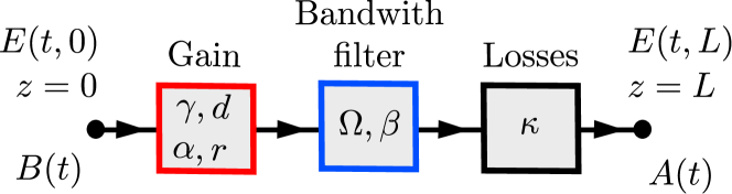
Figure 1: Schematic representation of the lumped-element approach for the link containing the gain medium, passive section, and bandwidth limiting element.

Since the derivation of the model (1,2) follows closely [15], it is not reported here. We limit to explain the role of each term. The differential equation (1) corresponds to a filter with Lorenzian line shape $\beta\exp\left[(-\beta+i\Omega)\xi\right]$ of the input signal $\sqrt{\kappa}\exp\left[(1-i\alpha)G(t)/2\right]E(t-T,0)$, where $E(t-T,0)$ is the field entering the link $T$ time before, $\sqrt{\kappa}$ is the total attenuation through nonresonant linear intensity losses, and $\exp\left[(1-i\alpha)G(t)/2\right]$ is the amplification and phase-shift factor due to the semiconductor gain medium. The rate of change of the gain in equation (2) is proportional to the injection current $d$, the term $-G(t)$ describes the gain decay without emission with the rate $\gamma$. The expression $r\left(1-\mathrm{e}^{G(t)}\right)|E(t-T,0)|^{2}$ is the contribution of the electric field to the gain rate; it is proportional to the variation of the intensity during the passage through the link. For instance, if the electric field is amplified during the passage, i.e. $|E(t-T,0)|^{2}<|E(t,L)|^{2}$, then this term is negative, thus contributing to the gain decay. Notice that the structure of the final model does not depend on the spatial distribution of the pump density, which enters the final equation only via the integral $d$.

The minimal, ring configuration, periodic boundary condition $E(t,0)=E(t,L)$, was already considered in [15]. Here, we discuss true network configurations starting from the inclusion of passive links, which can be treated as input-output

$$E(t,L)=\mathbf{\sqrt{\kappa}}E\left(t-T,0\right),$$ (3)

where $T$ is the propagation time. This equation can be considered as a special case of equation (1) for $\beta\to\infty$ (infinite bandwidth) and $G=0$. At variance with active links, passive ones are allowed to be bidirectional, since counter-propagating waves do not mutually interfere. As we show later, some of the directions of the passive links are not involved in the stationary dynamics, and the corresponding propagating waves decay in time exponentially to zero. However, for the sake of completeness, we prefer to consider the general case of bidirectional propagations.

2.2 Connecting the links

The coupling circuit elements (splitters) transform the incoming electric fields ($A_{j}(t)$ variables) into suitable output fields $B_{j}(t)$. Here below, we refer to a specific but commonly used linear four-ports, $2\times 2$ power splitter, described by a scattering $4\times 4$ matrix $\mathsf{S}_{\text{sp}}$ with the following properties (see Fig. 2):

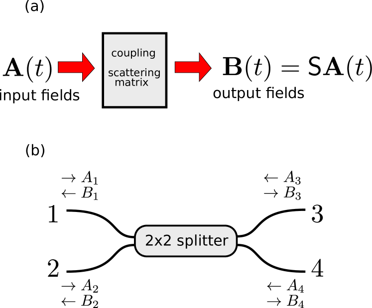
Figure 2: (a) General linear coupling between the links and (b) a particular realization with the 2x2 splitter.

1. Matched, i.e. no reflections, $\mathsf{S}_{\text{sp}}$ has $2\times 2$ block-diagonal structure;

2. Reciprocal (inversion symmetry, $\mathsf{S}_{\text{sp}}$ is symmetric): $\mathsf{S}_{\text{sp}}^{T}=\mathsf{S}_{\text{sp}}$ (the superscript $T$ denotes the transpose);

3. Lossless (energy conservation, $\mathsf{S}_{\text{sp}}$ is unitary): $\mathsf{S}_{\text{sp}}^{\dagger}=\mathsf{S}_{\text{sp}}^{-1}$.

Taking into account the above properties, $\mathsf{S}_{\text{sp}}$ can be written in the form [25]

$$\mathsf{S}_{\text{sp}}=\left(\begin{array}[]{cc}0&\mathsf{s}\\ \mathsf{s}^{T}&0\end{array}\right),$$ (4)

where

$$\mathsf{s}=\mathrm{e}^{i\phi}\left(\begin{array}[]{cc}\mathrm{e}^{i\psi_{1}}\cos\theta&\mathrm{e}^{i\psi_{2}}\sin\theta\\ -\mathrm{e}^{-i\psi_{2}}\sin\theta&\mathrm{e}^{-i\psi_{1}}\cos\theta\end{array}\right).$$ (5)

Here, $\theta$ measures the splitting ratio, $\psi_{1,2}$ the phase shifts in the splitting arms, and $\phi$ the overall splitter phase shifts. The $2\times 2$ sub-matrix $\mathsf{s}$ describes the input-output relation

$$\left(\begin{array}[]{c}B_{1}(t)\\ B_{2}(t)\end{array}\right)=\mathsf{s}\left(\begin{array}[]{c}A_{3}(t)\\ A_{4}(t)\end{array}\right)$$

for the output of the splitter given the input at the right ports 3 and 4, see Fig. 2. Similarly, $\mathsf{s}^{T}$ transforms the input from the left ports $A_{1}(t)$ and $A_{2}(t)$ into the output $B_{3}(t)$ and $B_{4}(t)$.

3 The LANER model

In order to define the LANER model, it is helpful to refer to a specific example such as the one depicted in Fig. 3. It is also useful to introduce two network representations. The first one is the physical network $\mathcal{P}$ (see panel (a)), whose nodes are the splitters, labelled by the index $k$, while the links are represented by the physical connections between pairs of splitters (self-connections are allowed), labelled by the index $m$. The second one, is the “abstract” network $\mathcal{A}$, whose nodes are the fields $A_{j}(t)$ observed at the end of each given link ($A_{j}(t)=E_{j}(t,L_{j})$, where $L_{j}$ is the length of the specific link). Hence, each active link is characterized by a single $A_{j}(t)$ variable (see, e.g. $A_{9}$ and $A_{10}$ in Fig. 3(a)). In passive links, bidirectional propagation is possible; hence we introduce two variables, $A_{j_{1}}(t)$ and $A_{j_{2}}(t)$ to represent counter-propagating waves (according to some unspecified rule): see e.g., the pairs $\left(A_{1},A_{2}\right)$, $\left(A_{3},A_{4}\right)$, $\left(A_{5},A_{6}\right)$, and $\left(A_{7},A_{8}\right)$ in Fig. 3(a).

The links of $\mathcal{A}$ encode the connections among the fields intervening in each splitter, see Fig. 3(b). For instance, consider node $A_{4}$ of the LANER network. Since the field $A_{4}$ affects the field $A_{9}$ through the splitter 2, there is a directed connection from $A_{4}$ to $A_{9}$. Similarly, the fields $A_{2}$ and $A_{10}$ affect $A_{4}$ through the splitter 1, leading to the connections $A_{2}\to A_{4}$ and $A_{10}\to A_{4}$. The resulting LANER network for our example is shown in Fig. 3(b).

As it will become progressively clear, this latter representation is more appropriate for the formulation of the dynamical equations. It is, nevertheless, necessary to introduce a formal relationship between the two representations. With reference to $\mathcal{A}$, its nodes can be ordered as we prefer. For the sake of simplicity, passive nodes (passive links in the physical network $\mathcal{P}$) are labelled by an index $j\leq N_{p}$, while $N_{p}<j\leq N$ refers to the active nodes in $\mathcal{A}$ (active links in $\mathcal{P}$). Once the ordering has been chosen, the mapping from $\mathcal{A}$ to $\mathcal{P}$ is determined by two functions $M(j)$ and $Q(j)$, where $M(j)$ identifies the physical link in $\mathcal{P}$, while $Q(j)=\pm 1$ denotes the corresponding propagation direction (the value $\pm 1$ can be assigned once for all in an arbitrary way but consistently all over the network). Inversely, given the physical link $m$ and the propagation direction $q$, the function $J(m,q)$ determines the corresponding node within $\mathcal{A}$.

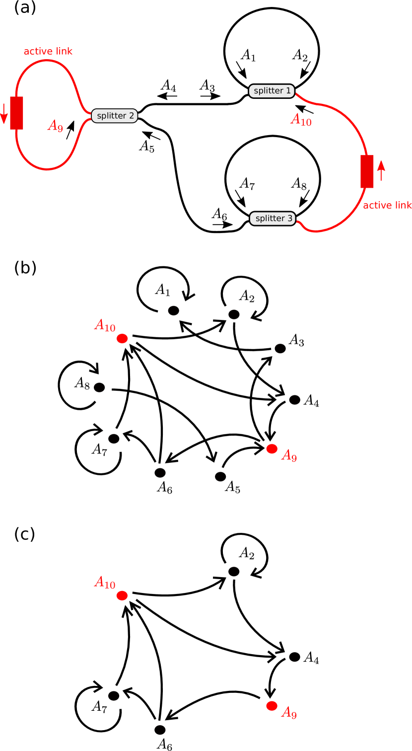
Figure 3: A LANER example. (a) the physical optical network. (b) the equivalent graph (the abstract LANER network). (c) the reduced graph determining the dynamics. Active links and fields are denoted in red, while passive in black.

From Eq. (3), the input-output relationship of the passive links are represented as

$$A_{j}(t)=\sqrt{\kappa_{j}}B_{j}\left(t-T_{j}\right)\;,\quad j=1,\dots,N_{p},$$ (6)

where $B_{j}(t)$ denotes the field amplitude at the beginning of the link (see Fig. 1).

The evolution of the active links follows instead from Eq. (1),

$$\frac{1}{\beta_{j}}\frac{dA_{j}(t)}{\partial t}=-\left(1-\frac{i\Omega_{j}}{\beta_{j}}\right)A_{j}(t)+\sqrt{\kappa_{j}}\mathrm{e}^{(1-i\alpha_{j})G_{j}(t)/2}B_{j}(t-T_{j})$$ (7)

$$\frac{1}{\gamma_{j}}\frac{dG_{j}(t)}{\partial t}=d_{j}-G_{j}(t)+r_{j}\left(1-\mathrm{e}^{G_{j}(t)}\right)|B_{j}(t-T_{j})|^{2},$$ (8)

$j=N_{p}+1,\dots,N$, where the subindex $j$ has been added to the parameters $\kappa$, $\alpha$, $\beta$, $d$, $\gamma$, $r$, and $T$ to stress that the various links differ in general from one another. Two-way propagation in active links cannot be modeled by the above equations, since the two fields interact with each other. In order to avoid the additional complications associated with such interaction, as anticipated, here in the following we assume unidirectional propagation along active links (such as in Fig. 3).

3.1 The scattering matrix

The equations can be closed by expressing the $B_{j}$ fields as functions of the $A_{j}$ variables. This is done, by including the action of the splitters in the model. Formally speaking, the transformation is linear and can be written in vector notations as

$${\bf B}(t)=\mathsf{S}{\bf A}(t),$$ (9)

where ${\bf B}=\left\{B_{j}\right\}_{j=1}^{N}$, ${\bf A}=\left\{A_{j}\right\}_{j=1}^{N}$, while $\mathsf{S}$ represents the scattering matrix, encoding the action of the splitters.

The structure of $\mathsf{S}$ can be determined from the contribution of the single splitters. Let $k=1,\dots,K$ be the index numbering the splitters, and let $a_{1}(k)$ be the input field from the network $\mathcal{A}$ entering the port 1 of the splitter $k$. Correspondingly, $a_{2}(k),a_{3}(k),$ and $a_{4}(k)$ are the fields entering the ports 2, 3, and 4. Similarly, we define $b_{1}(k)$, $b_{2}(k)$, $b_{3}(k)$, and $b_{4}(k)$ as the outgoing fields from the corresponding ports of the splitter $k$. The indices of the output fields can be determined by invoking the mapping between the links of network $\mathcal{P}$ and the nodes of $\mathcal{A}$,

$$b_{i}(k)=J[M(a_{i}(k)),-Q(a_{i}(k))]~{},~{}i=1,..,4~{}.$$ (10)

The relationships resulting in the example in Fig. 3 are presented in Table 1.

	$a_{1}$	$a_{2}$	$a_{3}$	$a_{4}$	$b_{1}$	$b_{2}$	$b_{3}$	$b_{4}$
$k=1$	1	3	2	10	2	4	1	-
$k=2$	-	9	4	5	9	-	3	6
$k=3$	7	6	8	-	8	5	7	10

Table 1: Definitions of the input-output fields for the splitters from the example in Fig. 3. $k$ numbers the splitters, $a_{j}$ is the input field into port $j$ and $b_{j}$ the outgoing field from the port $j$. The number is not defined if the propagation is unidirectional and there is no corresponding field.

From the structure of each $\mathsf{S}_{\text{sp}}$ matrix (see Eq. (4)) and the action of all splitters, it follows that the elements of the scattering matrix are

$$S_{j,l} = \sum_{k}\Bigl{\{}[\delta_{j,b_{1}(k)}\delta_{l,a_{3}(k)}+\delta_{j,b_{3}(k)}\delta_{l,a_{1}(k)}]\mathsf{s}_{1,1}(k)+$$ (11)

$$[\delta_{j,b_{1}(k)}\delta_{l,a_{4}(k)}+\delta_{j,b_{4}(k)}\delta_{l,a_{1}(k)}]\mathsf{s}_{1,2}(k)+$$

$$[\delta_{j,b_{2}(k)}\delta_{l,a_{3}(k)}+\delta_{j,b_{3}(k)}\delta_{l,a_{2}(k)}]\mathsf{s}_{2,1}(k)+$$

$$[\delta_{j,b_{2}(k)}\delta_{l,a_{4}(k)}+\delta_{j,b_{4}(k)}\delta_{l,a_{2}(k)}]\mathsf{s}_{2,2}(k)\Bigr{\}}.$$

In simple terms, all elements of the matrix $\mathsf{S}$ are equal to zero, except those which appear in the $k$th splitter transformation for some value of $k$. Since each link is assumed to end in a single well defined splitter, only one of the coefficients of the $\mathsf{s}$ elements can contribute to a given element of the matrix $\mathsf{S}$.

In the case of the LANER depicted in Fig. 3, the matrix $\mathsf{S}$ is

$$\mathsf{S}=\frac{1}{\sqrt{2}}\begin{bmatrix}1.&0.&-1.&0.&0.&0.&0.&0.&0.&0.\\ 0.&1.&0.&0.&0.&0.&0.&0.&0.&1.\\ 0.&0.&0.&0.&0.&0.&0.&0.&-1.&0.\\ 0.&-1.&0.&0.&0.&0.&0.&0.&0.&1.\\ 0.&0.&0.&0.&0.&0.&0.&-1.&0.&0.\\ 0.&0.&0.&0.&0.&0.&0.&0.&1.&0.\\ 0.&0.&0.&0.&0.&-1.&1.&0.&0.&0.\\ 0.&0.&0.&0.&0.&0.&0.&1.&0.&0.\\ 0.&0.&0.&1.&1.&0.&0.&0.&0.&0.\\ 0.&0.&0.&0.&0.&1.&1.&0.&0.&0.\end{bmatrix}$$

where we have assumed equal, $50\%$ splitters with zero phase delays, i.e., $\theta=\pi/4$ and $\phi=\psi_{1}=\psi_{2}=0$.

In the next subsection we derive the dynamical equations, determining the behavior of the LANER network. However, the network structure alone provides already important insight in the system properties. A moment’s reflection shows that the network depicted in Fig. 3(b) can be decomposed into three logically concatenated subnetworks, $\mathcal{N}_{1},\mathcal{N}_{2},$ and $\mathcal{N}_{3}$. The subnetwork $\mathcal{N}_{1}$ is composed of the nodes $A_{8}$ and $A_{5}$, and it is not influenced by the rest of the network. Moreover, being entirely passive, its action eventually vanishes and can be discarded, as shown in Fig. 3(c). Analogously, but with an opposite causality motivation, $\mathcal{N}_{3}$, composed of the nodes $A_{1}$ and $A_{3}$ does not influence the remaining six nodes composing $\mathcal{N}_{2}$: it is only forced by them in a master-slave configuration.

As a result, the bulk of the evolution arises from the fully connected component $\mathcal{N}_{2}$ .

3.2 LANER equations

Eqs. (9,11) allow expressing the field ${\bf B}$ in terms of ${\bf A}$ and, thereby closing the evolution equations (6), which can be rewritten in vector notations,

$$\boldsymbol{A_{p}}=\mathsf{K}_{p}\mathsf{P}\mathcal{T}\mathsf{S}\boldsymbol{A},$$ (12)

where $\boldsymbol{A_{p}}=\left[A_{1},\dots,A_{N_{p}}\right]^{T}$ refers to the fields in the passive links, $\mathsf{K}_{p}=\text{diag}\left\{\sqrt{\kappa_{1}},\dots,\sqrt{\kappa_{N_{p}}}\right\}$ represents the losses in the passive network part, $\mathsf{P}$ is the projector onto the passive links and, finally, $\mathcal{T}$ is the linear time-delay operator such that $\left[\mathcal{T}\boldsymbol{B}\right]_{j}=B_{j}(t-T_{j})$.

Similarly, we can eliminate ${\bf B}$ from Eqs. (7,8) and rewrite them as

$$\mathsf{C}\frac{d\boldsymbol{A}_{a}}{dt}=-\left[\boldsymbol{\text{I}}-i\mathsf{C}\mathsf{\Omega}\right]\boldsymbol{A}_{a}+\mathsf{F}_{1}(\boldsymbol{G})(\mathsf{I}-\mathsf{P})\mathcal{T}\mathsf{S}\boldsymbol{A},$$ (13)

$$\mathsf{D}\frac{d\boldsymbol{G}}{dt}=\boldsymbol{D}-\mathsf{F}_{2}(\boldsymbol{G})\left[\left((\mathsf{I}-\mathsf{P})\mathcal{T}\mathsf{S}\boldsymbol{A}\right)\circ\left((\mathsf{I}-\mathsf{P})\mathcal{T}\mathsf{S}\boldsymbol{A}\right)^{*}\right],$$ (14)

where $\boldsymbol{A}_{a}=\left[A_{N_{p}+1},\dots,A_{N}\right]^{T}$ are the fields for the active network parts, $\boldsymbol{G}=\left[G_{N_{p}+1},\dots,G_{N}\right]$ are the gains for the active links, $\mathsf{C}=\text{diag}\left\{\beta_{j}^{-1}\right\}_{j=N_{p}+1}^{N}$ and $\mathsf{D}=\text{diag}\left\{\gamma_{j}^{-1}\right\}_{j=N_{p}+1}^{N}$ are photon and gain timescales for the active part, $\boldsymbol{D}=\left[d_{j}\right]_{j=N_{p}+1}^{N}$ is the vector of the rescaled injection currents, $\mathsf{\Omega}=\text{diag}\left\{\Omega_{j}\right\}_{j=N_{p}+1}^{N}$ are frequencies of the spectral filtering for active links, $\mathsf{F}_{1}\left(\boldsymbol{G}\right)=\text{diag}\left\{\sqrt{\kappa_{j}}e^{(1-i\alpha_{j})G_{j}/2}\right\}_{j=N_{p}+1}^{N}$ and $\mathsf{F}_{2}\left(\boldsymbol{G}\right)=\text{diag}\left\{r_{j}\left(1-e^{G_{j}}\right)\right\}_{j=N_{p}+1}^{N}$ are nonlinear gain functions. Finally, the symbol $\circ$ denotes the component-wise multiplication.

From the representation (12)–(14), we see that the first two equations are linear in $\boldsymbol{A}$ – the action of the passive part of the network is given by the linear operator $\mathsf{K}_{p}\mathsf{P}\mathcal{T}\mathsf{S}$ involving time delays and a matrix multiplication – while the active subnetwork is essentially nonlinear. The system also possesses $S^{1}$ symmetry $\boldsymbol{A}\to\boldsymbol{A}e^{i\varphi}$, $\varphi\in S^{1}$ which is common for laser systems. The resulting system involves delay differential equations (13)–(14) as well as algebraic conditions (12). Such delay-differential-algebraic equations appear recently in a model for certain laser systems [26] and they are the subject of emerging theoretical research [27, 28].

A peculiarity of the model is the presence of two types of “oscillators”: active ones, characterized by two variables, and “passive” ones described by algebraic relations with time-shifts (without time derivatives). This is reminiscent of Boolean chaos [29, 30, 31, 32, 33], where all equations involve time-shifts and no “filtering” by time-derivatives. Here, only a subset of variables follows such a kind of dynamical evolution. As for the network structure, the links in $\mathcal{A}$ are all directed: each node can have at most two outgoing links and two (different) incoming ones.

In the zero delay limit, the evolution equations of the active links (see Eqs. (7,8)) reduce to ODEs, while passive links, determined by the Eq. (12), reduce to (linear) algebraic conditions, meaning that they can be eliminated from the evolution equations. As a result, in this limit, the LANER dynamics is equivalent to a network of $N-N_{p}$ oscillators (the active links) each oscillator being described by three variables (the two components of the field amplitude, plus the population inversion). In a sense, the model would be not too dissimilar from ensembles of either Lorenz or Rössler oscillators, both characterized by the same number of variables. An important difference is however in the phase-shift symmetry, which is typical for laser models [34, 23]. As a result, the single oscillator cannot be chaotic, and complex dynamics can arise due to interactions. The properties of the zero-delays model are most close to the rate equation models for semiconductor diodes, or compound cavity lasers [35, 36, 37, 38].

4 Networks with a single active link

Because of the presence of nonlinear elements, LANER systems are expected to exhibit a rich and complex dynamics. In order to clarify the role of passive network sections, see Fig. 4, in this section we analyse setups characterized by a single active (nonlinear) link.

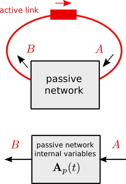
Figure 4: Single active medium LANER configuration.

Since we have a single active medium, to simplify notations in this section we use letters without subscript for the field $A$ (instead of $A_{N}$), the population inversion $G$, and for all other parameters of the active link. The scattering (coupling) matrix can be written in the block form as

$$\mathsf{S}=\left[\begin{array}[]{cc}\mathsf{S}_{p}&\mathbf{S}_{1}\\ {\bf S}_{2}^{T}&s\end{array}\right]$$ (15)

where $\mathsf{S}_{p}$ is a $P\times P$ matrix representing the connections between the passive links; ${\bf S}_{1}$ and ${\bf S}_{2}$ are two $P$-dimensional vectors encoding the connections between passive and active links. Finally the scalar $s$ accounts for the self-interaction present when the active link is closed onto itself.

As a result, the passive (algebraic) part of the dynamical equation, Eq. (12), can be written as

$${\bf A}_{p}=\mathsf{K}_{p}\mathcal{T}\left(\mathsf{S}_{p}\mathbf{A}_{p}+\mathbf{S}_{1}A\right).$$ (16)

Analogously, the two differential equations describing the active link are

$$\frac{1}{\beta}\frac{dA(t)}{dt}=-\left(1-\frac{i\Omega}{\beta}\right)A(t)+\sqrt{\kappa}\mathrm{e}^{(1-i\alpha)G(t)/2}B(t-T),$$ (17)

$$\frac{1}{\gamma}\frac{dG(t)}{dt}=d-G(t)+r\left(1-\mathrm{e}^{G(t)}\right)|B(t-T)|^{2},$$ (18)

where $B(t)$ represents the field amplitude at the beginning of the active link and is given by

$$B(t)=sA(t)+{\bf S}_{2}^{T}{\bf A}_{p}(t),$$ (19)

see Eqs. (9) and (15). Expressions (16)–(19) comprise the complete set of equations determining the dynamics of the setup in Fig. 4.

There is a variety of possible configurations of LANERs with one active link. Due to the nonlinearities, time-delays, possible complex coupling structure encoded in the coupling matrix $\mathsf{S}$, the description of their dynamical properties is interesting but infeasible in complete generality. Therefore, here we restrict our consideration to the solutions with stationary intensity of the form

$$A=\bar{A}\mathrm{e}^{i\omega t},\quad G=\bar{G},\quad\mathbf{A}_{p}=\bar{{\bf A}}_{p}\mathrm{e}^{i\omega t}$$ (20)

with time-independent $\bar{A}$, $\bar{G}$, and $\bar{\boldsymbol{A}}_{p}$. We will call them stationary (LANER) solutions. Substituting (20) into the evolution equations (16)–(19), we obtain

$$\begin{array}[]{cc}&\frac{i\omega}{\beta}\bar{A}+\left(1-\frac{i\Omega}{\beta}\right)\bar{A}=\sqrt{\kappa}\mathrm{e}^{(1-i\alpha)\bar{G}/2-i\omega T}\left(s\bar{A}+{\bf S}_{2}^{T}\bar{{\bf A}}_{p}\right),\\ &\bar{G}=d+r\left(1-\mathrm{e}^{\bar{G}}\right)|s\bar{A}+\mathbf{S}_{2}^{T}\bar{\mathbf{A}}_{p}|^{2},\\ &\bar{\boldsymbol{A}}_{p}=\mathsf{K}_{\Omega}\left(\mathbf{S}_{1}\bar{A}+\mathsf{S}_{p}\bar{\mathbf{A}}_{p}\right),\end{array}$$ (21)

where $\mathsf{K}_{\Omega}=\text{diag}\left(\sqrt{k_{1}}\mathrm{e}^{-i\omega T_{1}},\dots,\sqrt{k_{n}}\mathrm{e}^{-i\omega T_{n}}\right)$.

The non-lasing state is trivially identified by $\bar{A}=0$, $\bar{\mathbf{A}}_{p}=0$, and $\bar{G}=d$. The lasing states can be determined starting from the last equation, which gives

$$\left(\mathsf{I}-\mathsf{K}_{\Omega}\mathsf{S}_{p}\right)\bar{\mathbf{A}}_{p}=\mathsf{K}_{\Omega}\bar{A}\mathbf{S}_{1}.$$

For physically relevant cases of $\kappa_{j}<1$, $j=1,\dots,N_{p}$, the matrix $\mathsf{I}-\mathsf{K}_{\Omega}\mathsf{S}_{p}$ is invertible, hence

$$\bar{{\bf A}}_{p}=\bar{A}\left(\mathsf{I}-\mathsf{K}_{\Omega}\mathsf{S}_{p}\right)^{-1}\mathsf{K}_{\Omega}\mathbf{S}_{1}.$$ (22)

Upon replacing $\bar{{\bf A}}_{p}$ from (22) in the first two equations of (21), we obtain

$$1+i\frac{\omega-\Omega}{\beta}=\sqrt{\kappa}\mathrm{e}^{(1-i\alpha)\bar{G}/2-i\omega T}R\left(\omega\right),$$ (23)

$$\bar{G}=d+r\left(1-\mathrm{e}^{\bar{G}}\right)\left|R(\omega)\right|^{2}\left|\bar{A}\right|^{2},$$ (24)

where the transfer function

$$R(\omega):=s+\mathbf{S}_{2}^{T}\left(\mathsf{I}-\mathsf{K}_{\Omega}\mathsf{S}_{p}\right)^{-1}\mathsf{K}_{\Omega}\mathbf{S}_{1}$$ (25)

accounts for the propagation within the passive part of the network, including the relative time-delays.

By equating the square moduli of both sides of Eq. (23), we obtain the expression for the stationary gain

$$\bar{G}(\omega)=\ln\left[1+\left(\frac{\omega-\Omega}{\beta}\right)^{2}\right]-\ln\kappa-2\ln|R(\omega)|.$$ (26)

Further, Eq. (24) leads to the following stationary field intensity

$$\left|\bar{A}\right|^{2}=\frac{\bar{G}(\omega)-d}{r\left(1-\mathrm{e}^{\bar{G}}\right)\left|R(\omega)\right|^{2}}.$$ (27)

Finally, the argument of Eq. (23) yields the condition for the frequencies

$$\omega=\frac{1}{T}\left(-\frac{\alpha}{2}\bar{G}(\omega)-\arg\left(1+i\frac{\omega-\Omega}{\beta}\right)+\arg R(\omega)\right)+\frac{2\pi k}{T},$$ (28)

where $k\in\mathbb{Z}$.

The dependence on the delays due to the propagation along the passive links is contained in $\arg R(\omega)$ which is the superposition of different “periods” $2\pi/T_{i}$, corresponding to the various passive links. In the limit case of the ring laser [39] (no passive links), $R(\omega)\equiv 1$. In the next section we consider the less trivial example of a double ring configuration, illustrating its stationary states.

5 A first non-trivial LANER: the double ring configuration

The simplest, non-trivial example of LANER is the configuration depicted in Fig. 5, with a single, directed link with propagation delay $T$, accompanied by a bidirectional passive link with delay $T_{2}$.

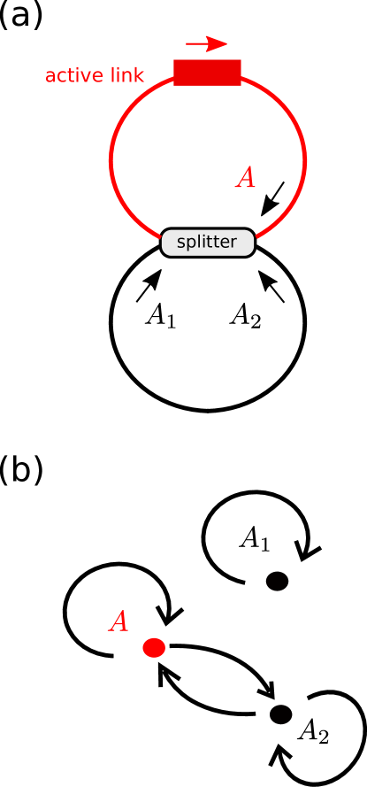
Figure 5: Double ring LANER with one active and one passive physical link. Physical network is shown in (a) and the corresponding abstract network in (b).

Similarly to the LANER with one active link in Sec. 4, $A(t)$ represents the field at the end of the active link and $G$ the corresponding gain variable. The equation for the active link is

$$\frac{1}{\beta}\frac{dA(t)}{dt}=-(1-i\frac{\Omega}{\beta})A(t)+\sqrt{\kappa}\mathrm{e}^{(1-i\alpha)G(t)/2}B(t-T),$$ (29)

$$\frac{1}{\gamma}\frac{dG(t)}{dt}=d-G(t)+r\left(1-\mathrm{e}^{G(t)}\right)|B(t-T)|^{2},$$ (30)

while for the passive link

$$A_{2}=\sqrt{\kappa_{2}}B_{2}\left(t-T_{2}\right).$$ (31)

The field $A_{1}$ is not coupled with the rest of the network. Since $A_{1}(t)=\sqrt{\kappa_{2}}B_{1}\left(t-T_{2}\right)=\sqrt{\kappa_{2}/2}A_{1}\left(t-T_{2}\right)$, its amplitude vanishes ($A_{1}(t)\to 0$) exponentially with time and it does not contribute to the stationary regime. Accordingly, such field could be removed from the very beginning in the model.

The coupling is described by the equation

$$\left(\begin{array}[]{c}B\\ B_{2}\end{array}\right)=\frac{1}{\sqrt{2}}\left(\begin{array}[]{cc}1&1\\ -1&1\end{array}\right)\left(\begin{array}[]{c}A\\ A_{2}\end{array}\right),$$

where we assume the splitter action to be 50% without phase delays. The final dynamical equations are

$$\frac{1}{\beta}\frac{dA(t)}{dt}=-(1-i\frac{\Omega}{\beta})A(t)+\\ \sqrt{\frac{\kappa_{3}}{2}}\mathrm{e}^{(1-i\alpha)G(t)/2}\left(A(t-T)+A_{2}(t-T)\right),$$ (32)

$$\frac{1}{\gamma}\frac{dG(t)}{dt}=d-G(t)+\frac{r}{2}\left(1-\mathrm{e}^{G(t)}\right)\left|A(t-T)+A_{2}(t-T)\right|^{2},$$ (33)

accompanied by the equation for the passive link

$$A_{2}(t)=\sqrt{\frac{\kappa_{2}}{2}}\left(-A(t-T_{2})+A_{2}(t-T_{2})\right).$$ (34)

In practice, this equation is a compact way to account for infinitely many delays.

Following the general approach of Sec. 4, for the stationary solutions

$$A_{j}=\bar{A}_{j}\mathrm{e}^{i\omega t},\qquad G=\bar{G}$$ (35)

the transfer function $R(\omega)$ of the passive part is

$$R(\omega)=\frac{1}{\sqrt{2}}\left(1-\sqrt{\frac{\kappa_{2}}{2}}e^{-i\omega T_{2}}\left(1-\sqrt{\frac{\kappa_{2}}{2}}e^{-i\omega T_{2}}\right)^{-1}\right).$$

Given $R(\omega)$, the stationary states can be determined from Eq. (28) for the frequency $\omega$, Eq. (26) for the gain $\bar{G}$, and Eq. (27) for the intensity $|\bar{A}|^{2}$.

A typical set of stationary states is presented in Fig. 6 for different parameter values. The blue lines show the dependence of the intensity $|A|^{2}$ in the active link on the frequency $\omega$, as from Eq. (27), irrespective whether the frequency is supported by the LANER setup. The dots denote the actual stationary states: the corresponding frequencies are determined by numerically finding the roots of the scalar equation (28).

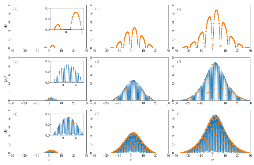
Figure 6: Stationary states (35) of the double-loop network for different parameter values. The points refer to the values of the intensity $|A|^{2}$ of the active link versus its frequency $\omega$. The blue line shows the dependence of $|A(\omega)|^{2}$ given by Eq. (27). Upper panel (a-c): $T=30$, $T_{2}=1$, and $d=0.5$ (a), $d=1.0$ (b), and $d=1.5$ (c). Middle panel (d-f): $T=2$, $T_{2}=7$, and $d=0.5$ (d), $d=1.0$ (e), and $d=1.5$ (f). Bottom panel (g-i): $T=21$, $T_{2}=13$, and $d=0.5$ (g), $d=1.0$ (h), and $d=1.5$ (i).

The various panels are arranged in the following way: rows identify different sets of propagation (delay) times $T$ and $T_{2}$; columns identify different values of the pump parameter $d$. More specifically, the upper row corresponds to a relatively long propagation time along the active link ($T=30\gg T_{2}=1$); in the middle row, the ratio is approximately opposite ($T=2<T_{2}=7$); finally, the lower row corresponds to comparable propagation times ($T=21$, $T_{2}=13$ – their ratio is an approximation of the golden mean). As for the columns, from left to right, $d=0.5$, 1, and 1.5, respectively. A first obvious consideration is that upon increasing the pump amplitude (i.e. moving from left to right), the number of active modes increases (see the range of possible frequencies) as well as their amplitude. As in the standard multimode laser, the higher amplitude field modes are located around the optical center frequency $\Omega$. The spectrum is not symmetric around $\Omega$ if the linewidth enhancement factor $\alpha\neq 0$. By comparing the different rows, we see that the number of active modes grows with the time-delays. Moreover, we notice that the passive section determines the amplitude of the active modes, inducing a relatively high sensitivity of their frequency when $T_{2}$ is comparable to $T$.

The overall scenario can be traced back to the structure of the transfer function $R(\omega)$. In Fig. 7, we separately plot modulus (upper panel) and phase (bottom panel) of $R(\omega)$ for the same delays as in the first row of Fig. 6. Since the passive part is composed of a single link, $R(\omega)$ is periodic of period $2\pi/T_{2}$. As $T\ll T_{2}$, the variation of $R(\omega)$ is slow compared over $\delta\omega=2\pi/T$, so that the distance between the active modes is approximately equal to $2\pi/T$. Moreover, we see that the intensity drops in correspondence of the minima of the transfer function, while the local maxima of the field intensity are located in the vicinity of the maxima of $\left|R(\omega)\right|$ as well as of the zeros of the phase $\arg R(\omega)$; this corresponds to an optimal transfer function for the minimal attenuation and no phase delay of the passive section.

For larger $T_{2}$, the spacing is more irregular. In particular, if $T_{2}\ll T$, it is the length of the passive link, which determines the average mode spacing (see the middle row in Fig. 6).

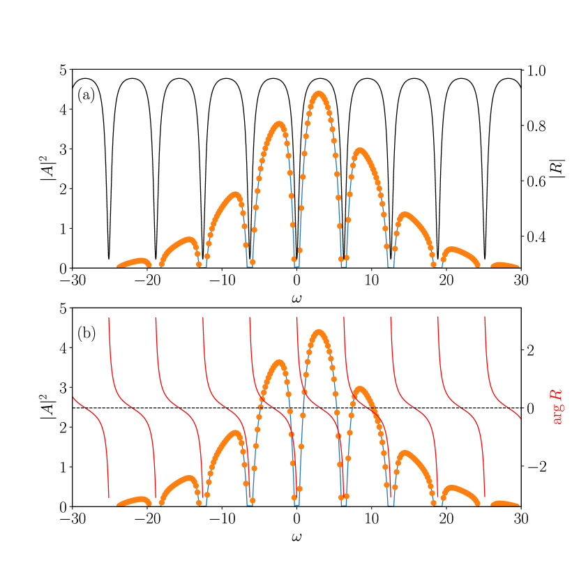
Figure 7: Modulus $|R(\omega)|$ (panel (a), black line, right axis) and phase $\arg R(\omega)$ (panel (b), red line, right axis) of the transfer function of the passive section compared to the intensity of the field $A$. Parameter values: $T=30$, $T_{2}=1$, and $d=1.5$.

6 Conclusions and future perspectives

In this paper we have introduced a formalism for the study of networks whereby waves with different frequencies propagate and interfere with one another, according to resonances implicitly selected by the network structure. As a result, we are able to study physical networks composed of both active and passive links, where the waves can be either amplified or damped. The dynamical system is represented as an abstract network whose nodes correspond to the electric fields propagating along the physical links, while its links correspond to the splitters which couple incoming with outgoing fields.

This formalism can be considered as an extension of the method developed to analyse quantum graphs to a context where wave propagation is nonlinear and in the presence of both gain and losses. Under the simplifying assumption of a linear damped propagation along the passive links, the corresponding dynamics can be treated as delayed boundary conditions.

In this paper we restricted the analysis to setups composed of a single active link. In such cases, the action of the passive subnetworks can be schematized through the action of a possibly complex transfer function, which contributes to select the active degrees of freedom, in principle, “offered” by the amplification along the single active link. The potential high dimensionality of the resulting dynamics is ensured by the delayed character of the equations. In the presence of multiple active links, we expect additional peculiarities to emerge because of the interactions between them. This challenging task goes, however, beyond the scope of the present work, which is mostly methodological.

From the point of view of the model, a relevant assumption that has helped simplifying its mathematical structure is the adiabatic elimination of the atomic polarization. This is a legitimate approximation in the context of semiconductor lasers, but much less so for, e.g. erbium doped optical fibers. A relevant step forward would be the extension of the formalism to such systems. This objective can in principle be achieved by explicitly including the spatial dependence along the active links; however the corresponding computational complexity would be so high as to make their analysis practically unfeasible. The true question is indeed under which conditions it is possible to keep a spaceless mathematical structure, integrating out the spatial dependence of the fields. This is a nontrivial step. Already in the context of semiconductor lasers, it should be noted that our equation of reference, used to describe an active link (see Eq. (1)) is partially phenomenological. As shown by Vladimirov and Turaev [15], the spatial integration of the population inversion leads to an algebraic delay equation, which exhibits time singularities under the form of high frequency instabilities. The proposed solution, also adopted herewith consists in the introduction of a filter (schematized by the time derivative of the field and identified by the bandwidth $\beta$), which regularizes the overall evolution.

This problem is reminiscent of the difficulty which emerges in a relatively similar class of models proposed more than ten years ago to describe an ensemble of dynamical units (the network nodes) which perform instantaneous Boolean operations in the absence of an external clock which synchronizes the single operations (see Ghil et al. [29]). The resulting mathematical model consists of a set of standard (non-differential) delay equations, where, like here, the delays originate from the transmission times along the single links. In such a context, an unphysical ultraviolet divergence appears as a consequence of the assumption of the instantaneous response of the single devices. Also in that case, the evolution equation has been phenomenologically regularized by turning it into a differential equation.

Besides the extension of our formalism to a still wider class of optical networks, another direction worth exploring is the actual dynamical regimes that can arise within the current context. In this paper, we have limited ourselves to determining the (many) stationary solutions. What about their stability and the onset of irregular dynamics because of the mutual nonlinear interactions? Finally, useful information and hints can instead arise from the analysis of a simpler setup: the zero-delay limit, as the LANER reduces to a network of 3-d coupled oscillators with phase-shift symmetry: it would be interesting to see to what extent its dynamics differs from that of similar dynamical systems, more extensively studied in the literature.

References

References

- [1] W. Gerstner, W. M. Kistler, R. Naud, L. Paninski, Neuronal dynamics: From single neurons to networks and models of cognition, Cambridge University Press, 2014. doi:10.1017/CBO9781107447615.
- [2] T. Nishikawa, A. E. Motter, Comparative analysis of existing models for power-grid synchronization, New Journal of Physics 17 (1) (2015) 015012. doi:10.1088/1367-2630/17/1/015012.
- [3] J. F. Donges, Y. Zou, N. Marwan, J. Kurths, Complex networks in climate dynamics, The European Physical Journal Special Topics 174 (1) (2009) 157–179. doi:10.1140/epjst/e2009-01098-2.
-
[4]
P. Kuchment, Quantum graphs: An
introduction and a brief survey, in: P. Exner, J. P. Keating, P. Kuchment,
T. Sunada, A. Teplyaev (Eds.), Analysis on graphs and its applications,
American Mathematical Society, Providence, 2008, pp. 291–312.
arXiv:0802.3442,
doi:10.1090/pspum/077/2459876.
URL http://www.ams.org/pspum/077 - [5] Y. Kuramoto, Chemical Oscillations, Waves, and Turbulence, Springer, Berlin, 1984.
- [6] T. Gross, B. Blasius, Adaptive coevolutionary networks: a review, Journal of The Royal Society Interface 5 (20) (2008) 259–271. doi:10.1098/rsif.2007.1229.
- [7] T. Aoki, T. Aoyagi, Self-organized network of phase oscillators coupled by activity-dependent interactions, Phys. Rev. E 84 (6) (2011) 66109. doi:10.1103/physreve.84.066109.
- [8] R. Berner, E. Schöll, S. Yanchuk, Multiclusters in Networks of Adaptively Coupled Phase Oscillators, SIAM Journal on Applied Dynamical Systems 18 (4) (2019) 2227–2266. doi:10.1137/18M1210150.
- [9] L. F. Abbott, S. B. Nelson, Synaptic plasticity: Taming the beast, Nature Neuroscience 3 (11s) (2000) 1178–1183. doi:10.1038/81453.
- [10] R. Zillmer, R. Livi, A. Politi, A. Torcini, Stability of the splay state in pulse-coupled networks, Phys. Rev. E 76 (4) (2007) 46102. doi:10.1103/PhysRevE.76.046102.
- [11] M. Gaio, D. Saxena, J. Bertolotti, D. Pisignano, A. Camposeo, R. Sapienza, A nanophotonic laser on a graph, Nature Communications 10 (1) (2019) 226. doi:10.1038/s41467-018-08132-7.
- [12] S. Lepri, C. Trono, G. Giacomelli, Complex active optical networks as a new laser concept, Physical Review Letters 118 (12) (2017) 123901. doi:10.1103/PhysRevLett.118.123901.
- [13] G. Giacomelli, S. Lepri, C. Trono, Optical networks as complex lasers, Physical Review A 99 (2) (2019) 023841. doi:10.1103/PhysRevA.99.023841.
- [14] O. Hess, T. Kuhn, Maxwell-Bloch equations for spatially inhomogeneous semiconductor lasers. I. Theoretical formulation, Physical Review A 54 (4) (1996) 3347–3359. doi:10.1103/PhysRevA.54.3347.
- [15] A. G. Vladimirov, D. Turaev, Model for passive mode locking in semiconductor lasers, Physical Review A 72 (3) (2005) 033808. doi:10.1103/PhysRevA.72.033808.
- [16] A. L. Franz, R. Roy, L. B. Shaw, I. B. Schwartz, Effect of multiple time delays on intensity fluctuation dynamics in fiber ring lasers, Physical Review E 78 (1) (2008) 016208. doi:10.1103/PhysRevE.78.016208.
- [17] F. Leo, S. Coen, P. Kockaert, S.-P. Gorza, P. Emplit, M. Haelterman, Temporal cavity solitons in one-dimensional Kerr media as bits in an all-optical buffer, Nature Photonics 4 (7) (2010) 471–476. doi:10.1038/nphoton.2010.120.
- [18] C. Mou, R. Arif, A. Rozhin, S. Turitsyn, Passively harmonic mode locked erbium doped fiber soliton laser with carbon nanotubes based saturable absorber, Optical Materials Express 2 (6) (2012) 884. doi:10.1364/OME.2.000884.
- [19] T. Herr, V. Brasch, J. D. Jost, C. Y. Wang, N. M. Kondratiev, M. L. Gorodetsky, T. J. Kippenberg, Temporal solitons in optical microresonators, Nature Photonics 8 (2) (2014) 145–152. doi:10.1038/nphoton.2013.343.
- [20] A. Bednyakova, S. K. Turitsyn, Adiabatic Soliton Laser, Physical Review Letters 114 (11) (2015) 113901. doi:10.1103/PhysRevLett.114.113901.
- [21] B. Romeira, R. Avó, J. M. L. Figueiredo, S. Barland, J. Javaloyes, Regenerative memory in time-delayed neuromorphic photonic resonators, Scientific Reports 6 (1) (2016) 19510. doi:10.1038/srep19510.
- [22] X. Liu, X. Yao, Y. Cui, Real-Time Observation of the Buildup of Soliton Molecules, Physical Review Letters 121 (2) (2018) 023905. doi:10.1103/PhysRevLett.121.023905.
- [23] M. C. Soriano, J. García-Ojalvo, C. R. Mirasso, I. Fischer, Complex photonics: Dynamics and applications of delay-coupled semiconductors lasers, Reviews of Modern Physics 85 (1) (2013) 421–470. doi:10.1103/RevModPhys.85.421.
- [24] L. Larger, A. Baylón-Fuentes, R. Martinenghi, V. S. Udaltsov, Y. K. Chembo, M. Jacquot, High-Speed Photonic Reservoir Computing Using a Time-Delay-Based Architecture: Million Words per Second Classification, Physical Review X 7 (1) (2017) 011015. doi:10.1103/PhysRevX.7.011015.
- [25] D. M. Pozar, Microwave Engineering, 4th Edition, John Wiley & Sons, Inc, 2012.
- [26] C. Schelte, P. Camelin, M. Marconi, A. Garnache, G. Huyet, G. Beaudoin, I. Sagnes, M. Giudici, J. Javaloyes, S. V. Gurevich, Third Order Dispersion in Time-Delayed Systems, Physical Review Letters 123 (4) (2019) 043902. doi:10.1103/PhysRevLett.123.043902.
- [27] P. Ha, V. Mehrmann, A. Steinbrecher, Analysis of Linear Variable Coefficient Delay Differential-Algebraic Equations, Journal of Dynamics and Differential Equations 26 (4) (2014) 889–914. doi:10.1007/s10884-014-9386-x.
- [28] B. Unger, Discontinuity Propagation in Delay Differential-Algebraic Equations, The Electronic Journal of Linear Algebra 34 (2018) 582–601. doi:10.13001/1081-3810.3759.
- [29] M. Ghil, I. Zaliapin, B. Coluzzi, Boolean delay equations: {A} simple way of looking at complex systems, Physica D: Nonlinear Phenomena 237 (23) (2008) 2967–2986. doi:10.1016/j.physd.2008.07.006.
- [30] R. Zhang, H. L. D. de S.Cavalcante, Z. Gao, D. J. Gauthier, J. E. S. Socolar, M. M. Adams, D. P. Lathrop, Boolean chaos, Physical Review E 80 (4) (2009) 045202. doi:10.1103/PhysRevE.80.045202.
- [31] D. P. Rosin, D. Rontani, D. J. Gauthier, Synchronization of coupled Boolean phase oscillators, Physical Review E 89 (4) (2014) 042907. doi:10.1103/PhysRevE.89.042907.
- [32] J. Lohmann, O. D’Huys, N. D. Haynes, E. Schöll, D. J. Gauthier, Transient dynamics and their control in time-delay autonomous boolean ring networks, Physical Review E 95 (2) (2017) 22211. doi:10.1103/PhysRevE.95.022211.
- [33] L. Lücken, D. P. Rosin, V. M. Worlitzer, S. Yanchuk, Pattern reverberation in networks of excitable systems with connection delays, Chaos 27 (1) (2017) 13114. doi:10.1063/1.4971971.
-
[34]
A. Uchida, F. Rogister, J. García-Ojalvo, R. Roy,
Synchronization
and communication with chaotic laser systems, in: Progress in Optics, 2005,
pp. 203–341.
doi:10.1016/S0079-6638(05)48005-1.
URL https://linkinghub.elsevier.com/retrieve/pii/S0079663805480051 -
[35]
S. Yanchuk, K. R. K. Schneider, L. Recke,
Dynamics of two
mutually coupled semiconductor lasers: Instantaneous coupling limit,
Physical Review E 69 (5) (2004) 56221.
doi:10.1103/PhysRevE.69.056221.
URL https://link.aps.org/doi/10.1103/PhysRevE.69.056221 -
[36]
H. Erzgraber, S. Wieczorek, B. Krauskopf,
Dynamics of two
laterally coupled semiconductor lasers: Strong- and weak-coupling theory,
Phys. Rev. E 78 (6) (2008) 66201.
doi:10.1103/PhysRevE.78.066201.
URL http://link.aps.org/abstract/PRE/v78/e066201 - [37] Y. Kominis, V. Kovanis, T. Bountis, Controllable asymmetric phase-locked states of the fundamental active photonic dimer, Physical Review AarXiv:1709.03823, doi:10.1103/PhysRevA.96.043836.
-
[38]
T. Erneux, D. Lenstra,
Synchronization of Mutually
Delay-Coupled Quantum Cascade Lasers with Distinct Pump Strengths,
Photonics 6 (4) (2019) 125.
doi:10.3390/photonics6040125.
URL https://www.mdpi.com/2304-6732/6/4/125 - [39] L. N. Menegozzi, W. E. Lamb, Theory of a Ring Laser, Physical Review A 8 (4) (1973) 2103–2125. doi:10.1103/PhysRevA.8.2103.