Dynamical cloud formation traced by atomic and molecular gas

Abstract

Context. Atomic and molecular cloud formation is a dynamical process. However, kinematic signatures of these processes are still observationally poorly constrained.

Aims. Identify and characterize the cloud formation signatures in atomic and molecular gas.

Methods. Targeting the cloud-scale environment of the prototypical infrared dark cloud G28.3, we employ spectral line imaging observations of the two atomic lines HI and [CI] as well as molecular lines observations in ¹³CO in the 1–0 and 3–2 transitions. The analysis comprises investigations of the kinematic properties of the different tracers, estimates of the mass flow rates, velocity structure functions, a Histogram of Oriented Gradients (HOG) study as well as comparisons to simulations.

Results. The central IRDC is embedded in a more diffuse envelope of cold neutral medium (CNM) traced by HI self-absorption (HISA) and molecular gas. The spectral line data as well as the HOG and structure function analysis indicate a possible kinematic decoupling of the HI from the other gas compounds. Spectral analysis and position-velocity diagrams reveal two velocity components that converge at the position of the IRDC. Estimated mass flow rates appear rather constant from the cloud edge toward the center. The velocity structure function analysis is consistent with gas flows being dominated by the formation of hierarchical structures.

Conclusions. The observations and analysis are consistent with a picture where the IRDC G28 is formed at the center of two converging gas flows. While the approximately constant mass flow rates are consistent with a self-similar, gravitationally driven collapse of the cloud, external compression by, e.g., spiral arm shocks or supernovae explosions cannot be excluded yet. Future investigations should aim at differentiating the origin of such converging gas flows.

1 Introduction

Molecular clouds are formed out of the atomic phase of the interstellar medium (ISM). While models detailing the transition from the atomic to molecular phase exist (e.g., Franco & Cox 1986; Hartmann et al. 2001; Bergin et al. 2004; Krumholz et al. 2008, 2009; Sternberg et al. 2014; Bialy et al. 2017), the observational constraints of the molecular cloud formation processes are still not properly characterized. Of particular importance is the dynamic state of the clouds, i.e., whether they are dominated by converging gas flows that could create over-densities important for the atomic-to-molecular gas conversion (e.g., Koyama & Inutsuka 2000; Audit & Hennebelle 2005, 2010; Vázquez-Semadeni et al. 2011, 2019; Heitsch et al. 2005, 2006; Heitsch & Hartmann 2008; Banerjee et al. 2009; Clark et al. 2012; Gómez & Vázquez-Semadeni 2014; Motte et al. 2014; Heiner et al. 2015; Henshaw et al. 2016; Langer et al. 2017), or whether more quasi-static cloud contraction processes take place where ever increasing densities may be related to the phase transitions between the atomic and molecular gas (e.g., Elmegreen 1993; Williams et al. 2000; McKee & Ostriker 2007).

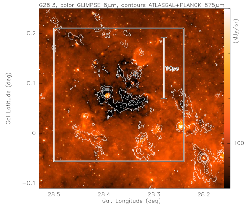
Figure 1: Overview of the target region G28.3. The color-scale presents the 8 $\mu$m emission from GLIMPSE (Churchwell et al., 2009), and the contours show the 875 $\mu$m emission from the ATLASGAL survey (Schuller et al. 2009, contour levels start at $4\sigma$ level of 200 mJy beam^-1 and continue in $8\sigma$ steps up to 1.8 Jy beam^-1). The white box outlines the approximate region imaged with APEX in the [CI] and ¹³CO(3–2) emission. A scale bar is shown within the box.

In dynamical pictures of converging gas flows, cloud-cloud collisions and cloud collapse flows, a convergence of gas flows towards some point in space is involved. A major difference between converging gas flows and cloud-cloud collisions on the one side, and cloud collapse on the other side is that in the converging gas flow and cloud-cloud collision picture the compression is produced by some external cause (e.g., supernovae or spiral arm potentials, e.g., Mac Low & Klessen 2004; Haworth et al. 2018; Kobayashi et al. 2018) whereas the collapsing cloud flows are dominated by the self-gravity of the cloud itself (e.g., Vázquez-Semadeni et al. 2019). In reality, externally driven converging flows may produce the clouds that then further collapse under their own self-gravity.

The observational characterization of the transition from atomic to molecular gas requires observations of both phases in atomic and molecular spectral lines, respectively. Most molecular cloud studies have been conducted in different lines of carbon monoxide covering a large range of spatial scales (e.g., Dame et al. 2001; Jackson et al. 2006; Dempsey et al. 2013; Barnes et al. 2015; Heyer & Dame 2015; Rigby et al. 2016; Umemoto et al. 2017; Schuller et al. 2017). Similarly, the HI 21 cm line has been observed a lot since its first detection (Ewen & Purcell, 1951), notable surveys of the Milky Way are Kalberla et al. (2005); Stil et al. (2006); McClure-Griffiths et al. (2009); Kerp et al. (2011); Winkel et al. (2016); HI4PI Collaboration et al. (2016); Beuther et al. (2016); Wang et al. (2019). However, kinematic studies of the HI emission are difficult because the spectra typically cover velocity ranges of 100 km s^-1 and more. With such broad line emission that traces a mixture of the cold neutral medium (CNM) and the warm neutral medium (WNM), unambiguous identification of velocity structure belonging to individual clouds is challenging (e.g., Kalberla & Kerp 2009; Winkel et al. 2016; Beuther et al. 2016; Murray et al. 2018; Wang et al. 2019). A different approach to study the atomic hydrogen kinematics is to look for HI self-absorption (HISA) features at comparably high HI column densities against HI background emission. Such HISA features allow us to isolate the CNM from the WNM. Some example studies in that direction were conducted by, e.g., Gibson et al. (2000, 2005a, 2005b); Li & Goldsmith (2003); Krčo et al. (2008); Heiner et al. (2015); Wang et al. (2020). In this work, we will employ the HI/OH/Recombination line survey of the Milky Way (THOR, Beuther et al. 2016; Wang et al. 2019) to study the HI kinematics from HISA features around the famous infrared dark cloud (IRDC) G28.3 (Fig. 1).

Neither molecular emission nor atomic HI emission trace the transition phase between the two media well. While the ionized carbon [CII] may trace that transition, [CII] emission depends on the local radiation field strength. In infrared dark clouds like the target cloud of this study, the [CII] emission is often too faint to be well detectable (e.g., Beuther et al. 2014; Clark et al. 2019). Furthermore, since [CII] cannot be observed from the ground, conducting large and sensitive maps are often difficult to obtain. Therefore, one of the arguably best tracers of the cloud formation and transition phase is the atomic carbon fine structure line [CI] around 492 GHz (e.g., Papadopoulos et al. 2004; Offner et al. 2014; Glover et al. 2015). The [CI] emission is believed to trace both the molecular clouds and also the more diffuse emission from the CO-dark molecular gas as well as the atomic envelope around the molecular clouds (e.g., Störzer et al. 1997; Papadopoulos et al. 2004; Offner et al. 2014; Glover et al. 2015).

Previous atomic carbon fine structure line studies typically covered only comparably small areas not extending far into the more diffuse cloud envelope structures (e.g., Keene 1995; Schilke et al. 1995; Ossenkopf et al. 2011). In an attempt to study the early evolutionary stages of high-mass star formation, we investigated four IRDCs in ionized, atomic and molecular carbon (Beuther et al., 2014). In one of the clouds (G48.66) we found evidence for converging gas flows in [CII] emission. However, even in that case, the size of the maps were comparably small not reaching far into the environmental cloud.

Here we are presenting an atomic carbon [CI] study of the prototypical IRDC G28.3 at scales larger of roughly $15^{\prime}\times 15^{\prime}$ or $\sim 20\times 20$ pc². The molecular cloud G28.3 is a large region where the innermost region is the well-known IRDC G28.3 (e.g.  Pillai et al. 2006; Wang et al. 2008; Ragan et al. 2012; Butler & Tan 2012; Butler et al. 2014; Tan et al. 2013; Tackenberg et al. 2014; Kainulainen & Tan 2013; Zhang et al. 2015; Feng et al. 2016b). Infrared data from the Spitzer satellite show that filamentary extinction structures extend from the large-scale atomic/molecular outskirts down to the innermost cloud center (Fig. 1, Churchwell et al. 2009). At a kinematic distance of 4.7 kpc, observations of the dense gas in N₂H⁺ indicate that the region is in a stage of global collapse (Tackenberg et al., 2014), and different signs of star formation activity exist throughout the cloud (e.g., Wang et al. 2008; Butler & Tan 2012; Tan et al. 2016; Feng et al. 2016a). The N₂H⁺(1–0) data of the central regions indicate already a velocity spread with peak velocities varying approximately between 77.5 and 81.5 km s^-1 (Tackenberg et al., 2014). In the following, we use as approximate velocity of rest $\varv_{\rm lsr}\sim 79.5$ km s^-1. The above characteristics make the G28.3 complex an ideal candidate to investigate the cloud formation and atomic to molecular gas conversion processes.

In the following, we combine an analysis from the diffuse environmental atomic and molecular cloud traced by HISA and ¹³CO(1–0) emission to the denser G28.3 IRDC center better studied in the [CI] and ¹³CO(3–2) transitions.

2 Observations and data

2.1 THOR HI and ¹³CO(1–0) GRS data

The HI data are taken from the HI/OH/Recombination lines survey of the Milky Way (THOR, Beuther et al. 2016; Wang et al. 2019) conducted with the Very Large Array (VLA). The final atomic hydrogen HI data product is the combined data cube from the THOR C-array observations with the previous VLA D-array survey and GBT single-dish data (VGPS, Stil et al. 2006). The angular and spectral resolution as well as the typical rms of the combined dataset are $40^{\prime\prime}$, 1.5 km s^-1 and 10 mJy beam^-1, respectively. For more details about the survey and data products, see Beuther et al. (2016), Wang et al. (2019) and the web-site at http://www.mpia.de/thor.

The corresponding large-scale ¹³CO(1–0) data are taken from the Galactic Ring Survey GRS, conducted with the FCRAO (Jackson et al., 2006). The spatial and spectral resolution as well as the typical rms sensitivity of this survey are $46^{\prime\prime}$, 0.21 km s^-1, and 0.13 K, respectively.

2.2 APEX [CI] and ¹³CO(3–2) observations

The atomic carbon [CI] and ¹³CO(3–2) data were observed with the APEX telescope in several observing runs between May and July 2018 (project ID M9504A_101). The approximate area of $0$ .${}^{\circ}25\times 0$ .${}^{\circ}25$ covered in the on-the-fly mode is outlined by the white box in Figures 1, 3 and 4. The two-band FLASH receiver was tuned to the [CI] frequency of 492.160651 GHz and to the ¹³CO(3–2) frequency of 330.587965 GHz. Maps were conducted in the on-the-fly mode doing always maps in Right Ascension and Declination to reduce potential scanning effects. The data reduction was conducted within the GILDAS framework with the sub-programs class and greg (for more details see http://www.iram.fr/IRAMFR/GILDAS).

The original spectral resolution is $\sim$0.05 km s^-1. However, to decrease the noise, we binned the data to a spectral resolution of 0.5 km s^-1. To increase the signal-to-noise ratio for the [CI] data, we smoothed them to a spatial resolution of $20^{\prime\prime}$. The ¹³CO(3–2) data are kept at their native spatial resolution of $18^{\prime\prime}$. The data are in antenna temperature $T_{A}^{*}$. The rms for the [CI] and ¹³CO(3–2) data-cubes in a single 0.5 km s^-1 channel is 0.14 and 0.12 K, respectively.

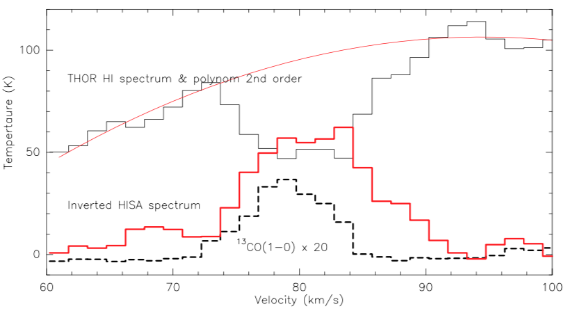
Figure 2: Compilation of HI and ¹³CO(1–0) spectra for the central area of the G28.3 IRDC (averaged over the central $100^{\prime\prime}$ squared). The thin black histogram shows the original HI emission data from the THOR survey (Beuther et al., 2016; Wang et al., 2019) where the HI self-absorption (HISA) is visible as absorption against the typically bright $\sim$100 K emission of the Galaxy. The red line presents a 2nd order polynomial fit to the non-HISA part of the spectrum. The red histogram then shows the resulting inverted HISA spectrum for this feature. The dashed histogram presents the ¹³CO(1–0) emission (Jackson et al., 2006) for the same region (multiplied by 20 for easier readability).

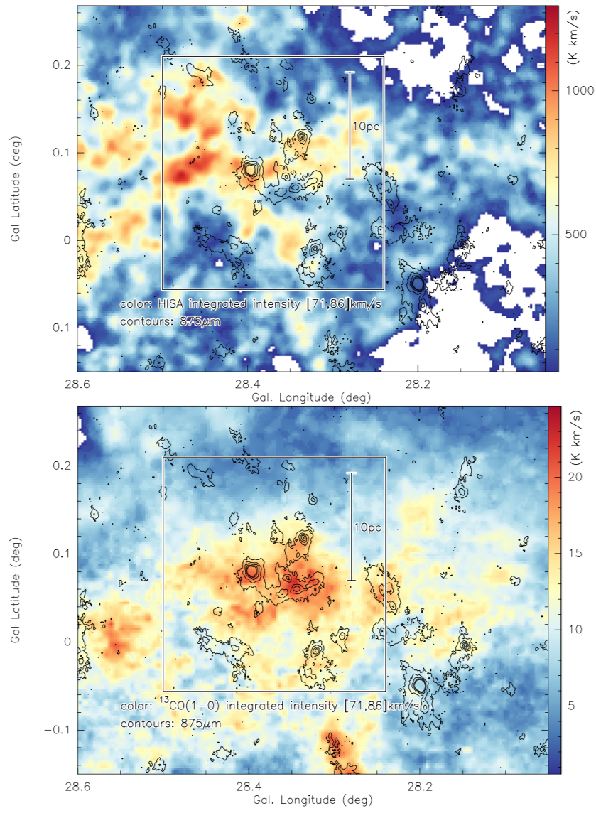
Figure 3: Large-scale structure of the cold neutral medium (CNM) measured as HISA in the THOR survey (top panel, Beuther et al. 2016; Wang et al. 2019, 2020) and the ¹³CO(1–0) emission from GRS (bottom panel, Jackson et al. 2006). The color-scales show the inverted HISA emission and ¹³CO(1–0) maps, respectively (integrated from 71 to 86 km s^-1 above 15 K in the HISA spectrum), and the contours show the 875 $\mu$m emission from the ATLASGAL survey (Schuller et al. 2009, contour levels start at $4\sigma$ level of 200 mJy beam^-1 and continue in $8\sigma$ steps up to 1.8 Jy beam^-1). The white box outlines the approximate region imaged with APEX in the [CI] and ¹³CO(3–2) emission. A scale bar is shown within the box.

3 Results

3.1 Large-scale atomic HI and molecular gas ¹³CO(1–0) distribution

The THOR atomic hydrogen data reveal a clear HI self-absorption (HISA) cloud in the environment of G28.3 (Figs. 2 and 3). While such a dip in HI emission could also be caused by missing HI, the fact that this HI emission dip at the given velocities is correlated with strong ¹³CO emission indicates that the lower HI emission is most likely caused by HI self-absorption (e.g., Riegel & Crutcher 1972; Heiles & Gordon 1975; van der Werf et al. 1988; Gibson et al. 2000; Kavars et al. 2005; Dénes et al. 2018; Wang et al. 2020). Furthermore, we checked the THOR cm continuum data for background sources against which we can measure directly the absorption. Although we have only weak continuum sources in that field prohibiting in-depth real absorption studies, we do find HI absorption against the continuum at the respective velocity ranges. This confirms high HI column densities and hence the HISA interpretation in general G28.3 cloud.

Since HISA features are absorption signatures against the bright HI emission of the Milky Way, they are tracing the CNM (e.g., Li & Goldsmith 2003; Gibson et al. 2000, 2005a, 2005b; Wang et al. 2020). Fitting a second order polynomial to the channels around the HISA feature, and inverting the resulting spectra, one can retrieve a HISA spectrum (see Fig. 2 showing the different parts of that approach). For more details about the actual HISA extraction process, see Wang et al. (2020).

In comparison to the normal HI spectrum with emission at almost all velocities, such a HISA spectrum has the advantage that it is almost Gaussian and allows us a much simpler analysis of the CNM than any normal HI emission spectra would do. Doing this HISA fitting pixel by pixel, one can derive a “HISA emission map”. Figure 3 presents this HISA map integrated over the velocity of the cloud between 71 and 86 km s^-1. One clearly sees that the general structure of the CNM traced by the HISA is associated with the infrared dark cloud G28.3, but that the CNM appears as expected to be more extended. While the central 875 $\mu$m emission appears to be embedded in a larger-scale envelope of CNM, the HISA peak emission is offset from the 875 $\mu$m main filamentary structure. This decrease of HISA towards the main infrared dark filament may be indicative of ongoing conversion of atomic to molecular gas in the central denser molecular cloud, also traced by the 875 $\mu$m emission.

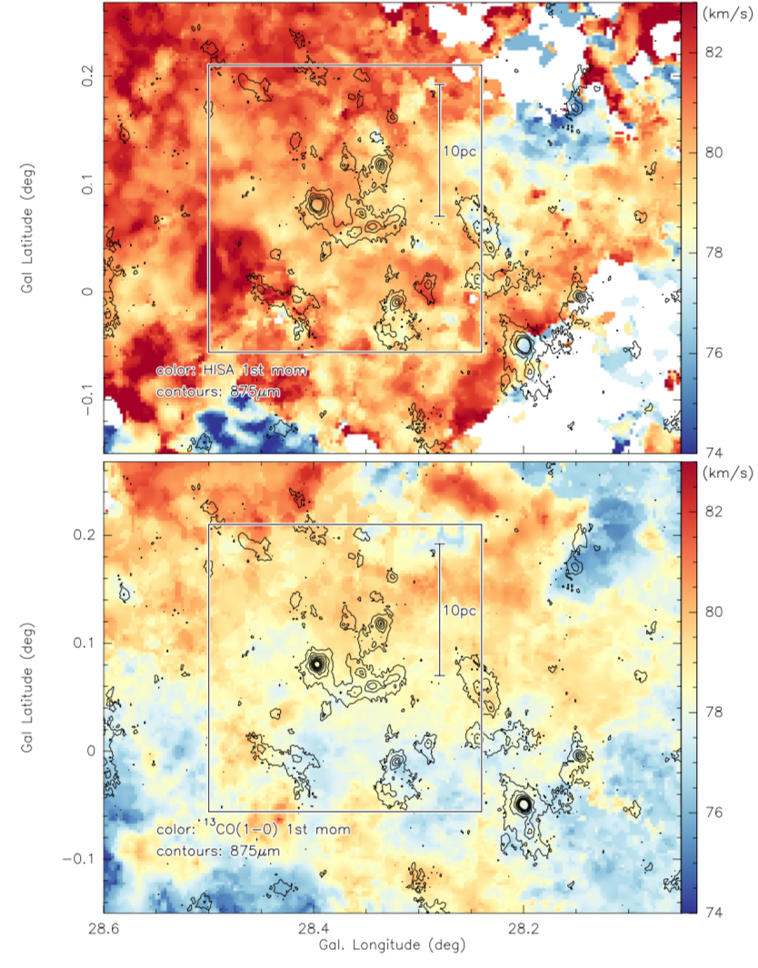
Figure 4: Large-scale velocity structure of the cold neutral medium (CNM) measured as HISA (top panel) and of the molecular gas measured in ¹³CO(1–0) (bottom panel, Jackson et al. 2006). The color-scale shows in both panels the 1st moment maps (intensity-weighted peak velocities), and the contours show the 875 $\mu$m emission from the ATLASGAL survey (Schuller et al., 2009), contour levels start at $4\sigma$ level of 200 mJy beam^-1 and continue in $8\sigma$ steps up to 1.8 Jy beam^-1). The white box outlines the approximate region imaged with APEX in the [CI] and ¹³CO(3–2) emission. Scale bars are shown within the box.

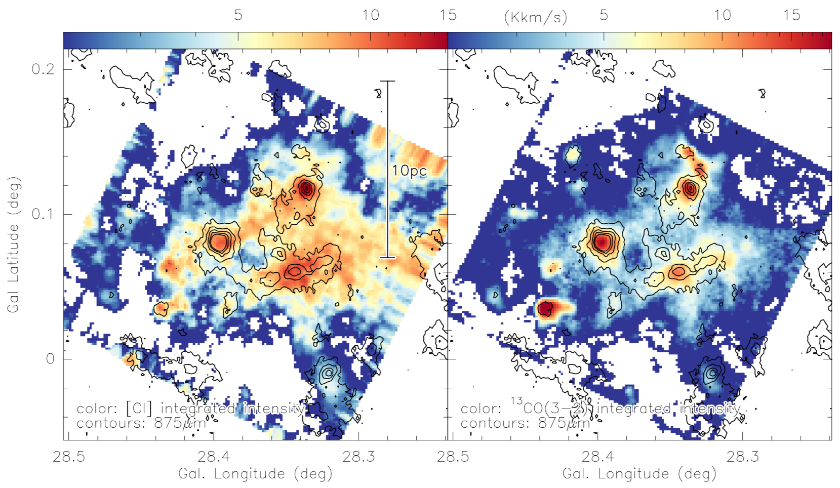
Figure 5: Integrated intensity maps of [CI] (left panel) and ¹³CO(3–2) (right panel). The color-scales present the corresponding integrated line maps over a velocity range of [71,86] km s^-1. The contours show the 875 $\mu$m emission from the ATLASGAL survey (Schuller et al. 2009, contour levels start at $4\sigma$ level of 200 mJy beam^-1 and continue in $8\sigma$ steps up to 1.8 Jy beam^-1). A scale bar is shown in the left panel.

Furthermore, one can use the HISA data cube and extract moment maps to study the velocity structure, similar to typical approaches conducted with molecular line data. Figure 4 presents the corresponding 1st moment maps (intensity-weighted peak velocities) of the HISA as well as the ¹³CO(1–0) data from GRS (Jackson et al., 2006). The general gas velocities of the CNM traced by the HISA and the molecular gas traced by the ¹³CO(1–0) emission cover the same velocities between approximately 70 and 90 km s (Figs. 2 & 4). Hence, both should trace approximately the same large-scale structures in our Milky Way. However, there are also significant kinematic differences: While the molecular gas shows a velocity gradient across Galactic latitudes (similar to the finding of the even denser gas seen in N₂H⁺ on smaller scales by Tackenberg et al. 2014) from $\sim$83 km s^-1 to $\sim$76 km s^-1, the HISA 1st moment map rather shows more uniform velocities around 82–83 km s^-1 in the outskirts of the cloud with slightly lower velocities toward the center of the G28.3 region. While this slight shift may be indicative of a small gradient also in the HISA map, this is observationally not significant (see also position-velocity discussion in section 3.2). We will get back to the velocity gradients in comparison to the [CI] emission in the following section.

3.2 Velocity structure of atomic and molecular carbon around the G28.3 IRDC

In the following, we focus on the closer environment around the IRDC G28.3. Figure 5 presents the integrated [CI] and ¹³CO(3–2) emission from our APEX observations. While both tracers show strongest emission toward the 875 $\mu$m peak positions, the ¹³CO(3–2) emission follows the dense gas structures more closely than the atomic carbon [CI] emission that exhibits a more diffuse halo-like structure around the central 875 $\mu$m dust continuum emission.

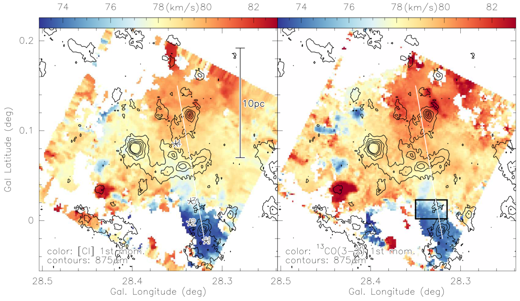
Figure 6: First moment maps (intensity-weighted peak velocities) of [CI] (left panel) and ¹³CO(3–2) (right panel). The color-scales present the corresponding integrated line maps over a velocity range of [71,86] km s^-1. The contours show the 875 $\mu$m emission from the ATLASGAL survey (Schuller et al. 2009, contour levels start at $4\sigma$ level of 200 mJy beam^-1 and continue in $8\sigma$ steps up to 1.8 Jy beam^-1). The white lines show the direction (north to south) of the pv-diagrams in Fig. 9. The stars in the left panel show the positions of the spectra presented in Fig. 8. A scale-bar is shown in the left panel. The little box in the right panel outlines the region with the velocity jump.

More interesting than just the integrated emission are the kinematic signatures found in both tracers. Fig. 6 shows the 1st moment maps in [CI] and ¹³CO(3–2). One can identify in both tracers a clear velocity gradient from roughly 83 km s^-1 at latitudes higher than the central IRDC, and velocities even below 74 km s^-1 at latitudes below the IRDC. The main dust continuum filament around a latitude of $\sim 0$ .${}^{\circ}07$ exhibits a rather uniform peak velocity around $\sim 78$ km s^-1. whereas the additional strong 875 $\mu$m peak at higher latitudes ($\sim 0$ .${}^{\circ}12$) is already more redshifted with velocities $>80$ km s^-1. This velocity shift was already identified in the high-density tracer N₂H⁺ by Tackenberg et al. (2014).

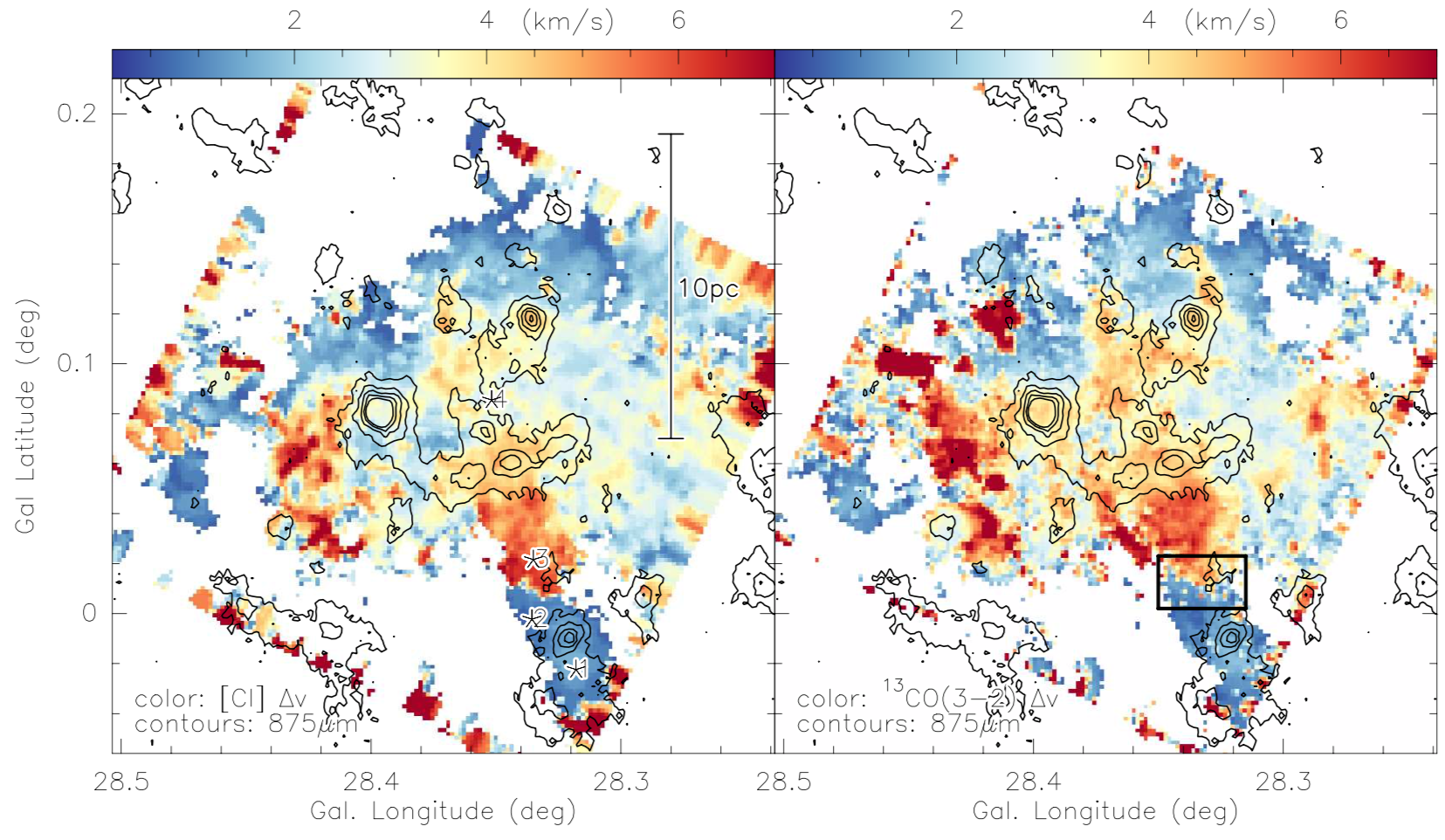
Figure 7: Second moment maps (intensity-weighted velocity dispersions) of [CI] (left panel) and ¹³CO(3–2) (right panel) over a velocity range of [71,86] km s^-1. The contours show the 875 $\mu$m emission from the ATLASGAL survey (Schuller et al. 2009, contour levels start at $4\sigma$ level of 200 mJy beam^-1 and continue in $8\sigma$ steps up to 1.8 Jy beam^-1). The stars in the left panel show the positions of the spectra presented in Fig. 8. A scale-bar is shown in the left panel. The little box in the right panel outlines the region with the velocity jump.

Particularly prominent is a velocity feature at Galactic coordinates of $\sim 28$ .${}^{\circ}33/0$ .${}^{\circ}01$ where the first moment maps in Fig. 6 show a strong decrease to even lower velocities, and at the same position the second moment maps exhibit almost a jump to low velocity dispersion measurements (see little box in Figs. 6 and 7). Since moment maps are only intensity-weighted integral measurements, to investigate this velocity change in more depth, we extracted individual [CI] and ¹³CO(3–2) spectra toward four positions along that velocity structure marked as “1” to “4” in Figures 6 and 7. These spectra are shown in Figure 8.

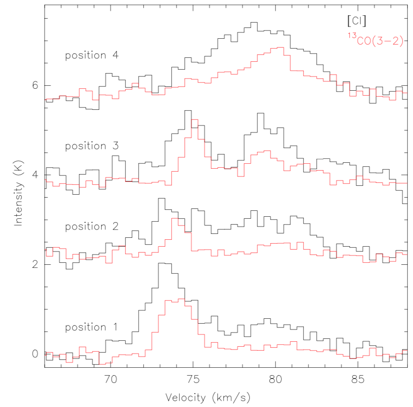
Figure 8: [CI] (black) and ¹³CO(3–2) (red) spectra toward the four positions marked in Figs. 6 and 7. The vertical y-axis offsets between the spectra are only for better readability.

The [CI] and ¹³CO(3–2) spectra toward that region clearly exhibit several velocity components. While the southernmost position “1” shows mainly one velocity component around 73-74 km s^-1, the northernmost position “4” is dominated by a (broader) component at around 79 km s^-1. The two positions inbetween, and particularly prominent toward position “3” show two component spectra combining the features seen individually toward positions “1” and “4”.

Having two different velocity components in the environment of that IRDC raises the question whether we are witnessing the potential interaction of two gas flows. These could be either externally driven colliding flows and/or cloud-cloud collisions, or they could be driven by self-gravity, that may trigger the formation of a dense star-forming molecular cloud at its converging point (e.g., Duarte-Cabral et al. 2011; Bisbas et al. 2017; Inoue et al. 2018; Kobayashi et al. 2018; Haworth et al. 2015, 2018; Vázquez-Semadeni et al. 2006; Heitsch et al. 2008; Banerjee et al. 2009; Gómez & Vázquez-Semadeni 2014; Vázquez-Semadeni et al. 2019). Regarding the externally driven processes, one can consider the cloud-cloud collisions as a sub-group of the more general colliding gas flows. The main difference should be the state of the gas: While colliding flows are in general considered to be continuous gas flows that start as more diffuse HI clouds with a mix of CNM and WNM, the cloud-cloud collision picture typically refers to more concrete objects consisting mainly of cold, molecular gas (e.g., Haworth et al. 2015, 2018; Bisbas et al. 2017).

To better evaluate such potential converging gas flows, Figure 9 presents position-velocity cuts along approximate north south direction in all four gas tracers, HI, ¹³CO(1–0), [CI] and ¹³CO(3–2). The corresponding cut directions for the two pairs of tracers (HI/¹³CO(1–0) for the larger scales, and [CI]/¹³CO(3–2) for the closer environment of the IRDC) are shown if Figs. 10 and 6, respectively. While for the larger-scale HISA and ¹³CO(1–0) data, we select the most straightforward north-south direction, for the [CI] and ¹³CO(3–2) emission, the cut is slightly inclined ($\sim$10⁰, Fig. 6) to follow the larger extent of the [CI] and ¹³CO(3–2) emission along that axis. We checked more orientations on the different data, and this small difference does not change the results discussed below. The orientation of the pv-diagrams is north-south, i.e., offset $0^{\prime\prime}$ is the northern end of the cut.

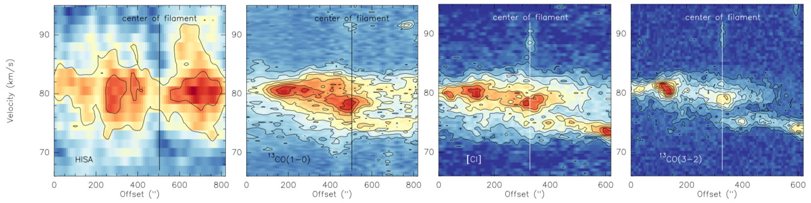
Figure 9: Position-velocity diagrams for the four tracers from left to right: HISA, ¹³CO(1–0), [CI] and ¹³CO(3–2). The cuts are in a north-south direction along the lines shown in Figs. 6 ([CI], ¹³CO(3–2)) and 10 (HISA, ¹³CO(1–0)). Both axes have slightly larger extent for the HISA and ¹³CO(1–0) data compared to the [CI] and ¹³CO(3–2) cuts. The approximate location of the center of the filament is marked in all panels.

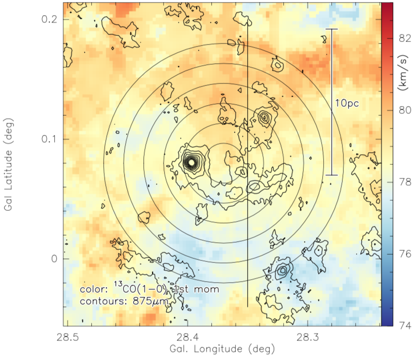
Figure 10: Zoom into the ¹³CO(1–0) 1st moment map from Fig. 4. The color-scale shows the 1st moment map, and the contours present the ATLASGAL 875 $\mu$m emission (Schuller et al., 2009), contour levels start at $4\sigma$ level of 200 mJy beam^-1 and continue in $8\sigma$ steps up to 1.8 Jy beam^-1). A scale bar is shown. The black line presents the direction (north to south) of the pv-diagrams in Fig. 9. The circles outline annuli with radii starting at $60^{\prime\prime}$ and then increasing in $60^{\prime\prime}$ steps to $360^{\prime\prime}$ (for details see section 4.3).

These pv-diagrams exhibit a few interesting features. To start with the diffuse emission, the HISA pv-diagram shows no obvious velocity gradient over the whole extent of $\sim 800^{\prime\prime}$ (roughly 18.25 pc at 4.7 kpc distance). Going to the molecular gas, the ¹³CO(1–0) cut peaks in the north at roughly 80.5 km s^-1, stays in that regime for about $300^{\prime\prime}$, and then exhibits a gradient toward the center of the filament to $\sim$77.5 km s^-1. Of particular interest is then also the regime south of the main filament where the ¹³CO(1–0) emission shows two components, one again around 80.5 km s^-1, and the second component at lower velocities of $\sim$74.5 km s^-1.

The two pv-diagrams for [CI] and ¹³CO(3–2) cover a slightly smaller length with about $600^{\prime\prime}$ or $\sim$13.7 pc. Around the central filament, they exhibit similar signatures with velocities around 80.5 km s^-1 in the north and even below 74 km s^-1 in the south. The filament itself shows again intermediate velocities between 77 and 79 km s^-1. While the overall signatures for [CI] and ¹³CO(3-2) are similar, [CI] shows a bit more extended emission with a larger velocity spread (see also Fig. 5). The division into separate velocity components is most prominent in the highest-density tracer ¹³CO(3-2). With the higher spatial and spectral resolution of the [CI]/¹³CO(3–2) data compared to the ¹³CO(1–0) data, one also more clearly resolves the gradient-like velocity structure of the two components from the north and the south toward the central filament.

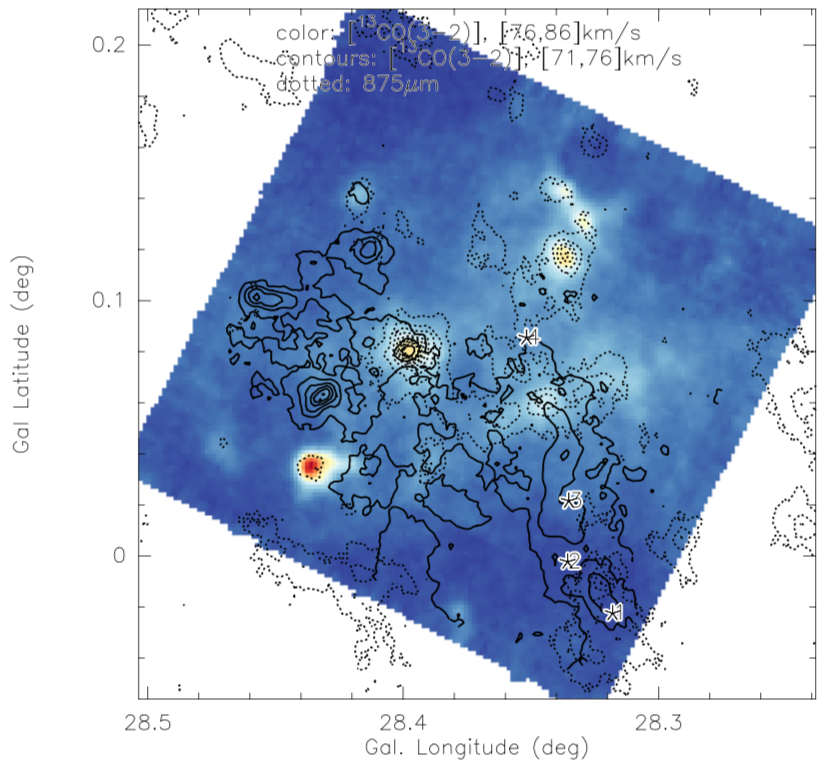
Figure 11: Integrated ¹³CO(3–2) emission for two velocity components. The color scale and full contours show the [76,86] and [71,76]km s^-1 components, respectively. The contour levels are in $9\sigma$ steps (with $1\sigma=0.125$ K km s^-1). The dotted contours show the corresponding 875 $\mu$m continuum emission from Schuller et al. (2009) as reference frame. The stars again show the positions of the spectra presented in Fig. 8.

For visualization purpose, Fig. 11 shows the ¹³CO(3–2) integrated emission maps for the two velocity regimes [71,76] km s^-1 and [76,86] km s^-1, respectively. Although there is no clear north-south separation of the two components, the higher-velocity gas is preferentially found toward the north and the lower-velocity gas more toward the south. One has to keep in mind that these gas components and kinematic signatures are always projections onto the plane of the sky, and therefore, clear spatial separations would even be a surprise.

We note that while the first moment maps of ¹³CO(1–0) and [CI]/¹³CO(3–2) (Figs. 4 and 6) give the visual impression that the velocity gradient may increase with critical density of the tracer, this is most likely mainly caused by the two velocity components and the fact that the second component around 74.5 km s^-1 is more pronounced in the higher density tracers [CI]/¹³CO(3–2). Closer inspection of the pv-diagrams in Fig. 9 for these three tracers, considering only the transition from the north to the center of the filament, show that there is no large difference in the magnitude of the velocity gradient. Similar velocity regimes were also found in the even higher-density tracer N₂H⁺(1–0) by Tackenberg et al. (2014).

Combining these different velocity signatures, the data show strong signatures of two gas components at different velocities (around 6 km s^-1 apart) that converge to a common intermediate velocity at the location of the infrared dark cloud and active star-forming region, similar to filament formation via gravitationally driven, converging gas flows (e.g., Gómez & Vázquez-Semadeni 2014). We interprete these signatures as indicators of converging gas streams that may trigger the star formation event at its center (e.g., Vázquez-Semadeni et al. 2006; Heitsch et al. 2008; Banerjee et al. 2009; Gómez & Vázquez-Semadeni 2014). Position-velocity diagrams based on simulations of cloud-cloud collisions sometimes show a characteristic pattern of lower-level emission between two main velocity components, a so-called bridging feature (e.g., Haworth et al. 2015, 2018). Similar signatures were also reported in observations (e.g., Jiménez-Serra et al. 2010; Henshaw et al. 2013; Dobashi et al. 2019; Fujita et al. 2019). The pv-diagrams of the G28.3 region presented here (Fig. 9) show different signatures in the sense that there is not a lower-intensity bridge between the two well-defined components, but that the two velocity components converge at the center of the cloud toward a central, high-intensity velocity component. However, the absences of a bridging feature does not necessarily rule out the formation of G28.3 in a cloud-cloud collision, as this feature is not always visible in simulations. For example, simulations by Bisbas et al. (2017) show that the low-intensity bridge feature may merge into a centrally peaked pv-diagram during the evolution of the cloud-cloud collisions while the colliding-cloud simulations of Clark et al. (2019) yield only a single central velocity component in CO or [CI], with multiple components only becoming apparent when one looks at the [CII] emission from the cloud. In addition to this, the multiple components and bridging feature may not be visible in cases where our line of sight is oriented at a large angle to the direction of motion of the clouds. We get back to the interpretation in sections 4.4 and 4.5.

4 Discussion

4.1 Histogram of Oriented Gradients (HOG)

A way to evaluate similarities in the structures traced by the different spectral lines is the histogram of oriented gradients (HOG), a statistical method from machine vision recently introduced in astrophysical data analysis by Soler et al. (2019). Basically, the HOG analysis compares intensity maps by comparing the relative orientation between its gradients. The degree of correlation between the images is estimated using the projected Rayleigh statistic ($V$), which is a test that quantifies if the relative angle distribution is flat, as it is the case of two completely uncorrelated maps, or peaked around 0 deg, as it is the case of two maps with a significant degree of correlation.

The HOG can be used to compare individual single-frequency maps, but also to position-position-velocity cubes. In that case, the result of the analysis is a matrix of $V$ values for the different velocity channels in each tracer, which is shown in Fig. 12. We use this matrix of $V$ values to investigate whether the gas traced by different spectral lines follows a similar spatial distribution across velocity channels. Soler et al. (2019) applied the HOG analysis to spectral line data as well as different simulations, and they found, for example, that constant converging gas flows result in spatial and kinematic structures agreeing well between different spectral lines (mainly showing high projected Rayleigh-V values along the diagonal in plots like those in Fig. 12), whereas feedback processes can produce kinematic offsets between, e.g., atomic and molecular gas (showing high projected Rayleigh-V values offset from the diagonal). For more details about the method and its implications, please see Soler et al. (2019).

We applied this HOG method to the four datasets studied here, namely, [CI], ¹³CO(1-0), ¹³CO(3-2), and HISA position-position-velocity cubes. The resulting correlations, quantified by $V$, are presented in Fig. 12. We find that the HISA does not show significant correlation with any of the other tracers across the velocity range between 70 and 90 km s^-1. In contrast to this, the other three tracers show high spatial correlation across velocity channels, evidenced by high $V$ values. The largest values of $V$ are concentrated along the diagonal of the correlation plot, that is, across the same line-of-sight velocity in each pair of tracers. This result is expected for tracers that are co-spatial and co-moving.

The low values of $V$ found in the comparison between the HISA and the other tracers indicate that there is no morphological correlation between CNM as traced by HISA and the other denser gas tracers across all measured velocity channels. This lack of correlation can be interpreted as an indication of the decoupling of the dense gas of the main cloud from the mostly atomic CNM in the more diffuse cloud envelope. This is slightly different to the morphological correlation found between HI and ¹³CO(1–0) emission in the molecular clouds studied in Soler et al. (2019). It appears that correlation or non-correlation between HI and denser gas tracers may not be universal but could be an indication of different evolutionary stages in this kind of objects. We note that for the G28.3 cloud studied here, the HISA itself is also weaker toward the central filamentary IRDC as visible in Figs. 3 and 9. If one interpretes this depression of HISA towards the center as a sign of potential gas conversion from atomic H to molecular H₂, this can be taken as further support for the kinematic decoupling of the CNM, as traced by HISA, and the molecular phase.

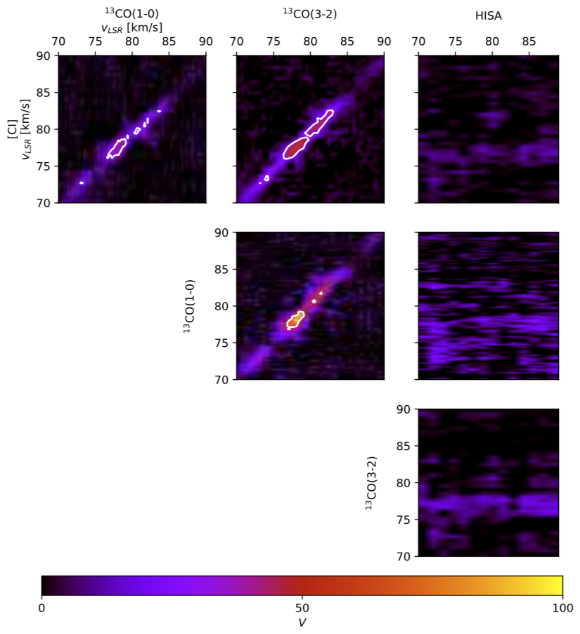
Figure 12: Spatial correlation between the four different tracers across velocity channels as evaluated using the histogram of oriented gradients method (HOG, Soler et al. 2019). The figure shows all tracers correlated with each other as labeled at each plot. The panels show the values of the projected Rayleigh statistic ($V$), a measure of the morphological correlation between velocity channels. Large values of $V$ indicate large correlation between the corresponding velocity-channels maps. The contours correspond to the 7 $\sigma$ confidence limit on the $V$ values, see Soler et al. (2019) for more details.

4.2 Velocity structure functions

A different way to investigate the kinematics of molecular clouds is the analysis of velocity structure functions (e.g., Miesch & Bally 1994; Ossenkopf & Mac Low 2002; Esquivel & Lazarian 2005; Heyer & Dame 2015; Chira et al. 2019; Henshaw et al. subm.). Velocity structure functions are essentially a measure of how much the velocity measured between pixels separated by a given distance varies as a function of spatial scale. Mathematically the structure function $S_{p}$ of order $p$ is described as:

$$S_{p}(l)=<|v(r)-v(r+l)|^{p}>$$

where $l$ is known as the spatial lag and represents the separation between pairs of points $S_{p}$ is calculated for. As outlined for example in Chira et al. (2019), the slope of the structure function can be used to infer whether turbulence and/or gravity play an important role in shaping the gas dynamics of the cloud. Chira et al. (2019) show in their simulations that purely turbulence-dominated structure functions are steeper than those where gravity becomes more important because gravity increases the velocity on small scales so that the structure function becomes shallower.

We now derived the velocity structure function $S_{2}$ of order 2 for all four gas tracers from their corresponding 1st moment maps (intensity-weighted peak velocities). To allow a meaningful comparison, the four 1st moment maps were smoothed to the $46^{\prime\prime}$ spatial resolution of the ¹³CO(1–0) data and all put on the same pixel grid. No large-scale gradient was removed from the data. Since we derived the structure function from the 1st moment maps, and these are intensity-weighted peak velocities, the derived structure functions can be considered as (column-)density weighted velocity structure functions.

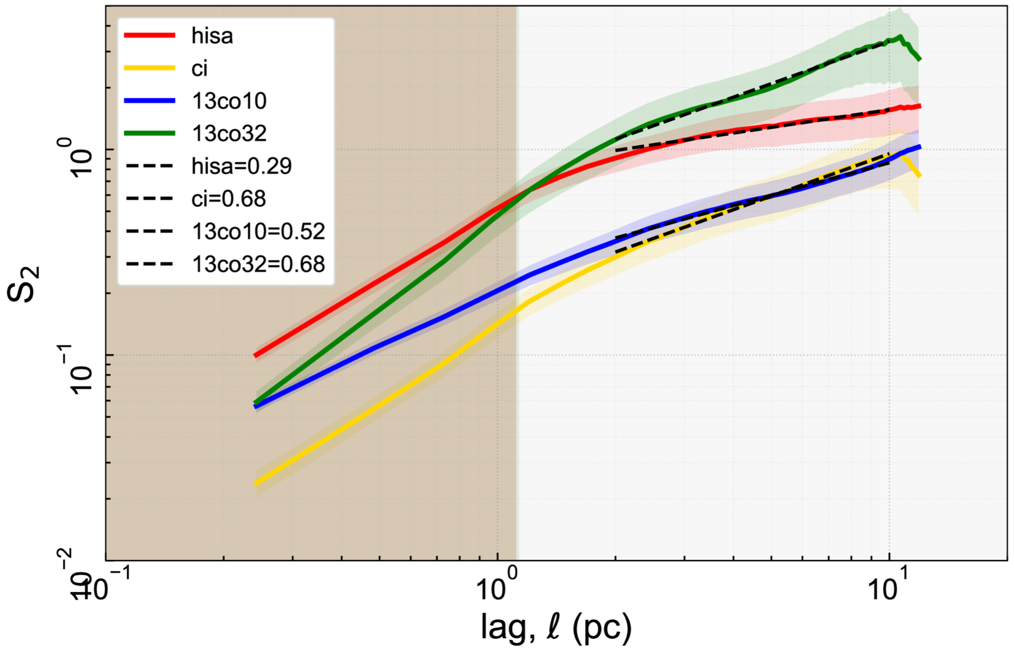
Figure 13: One-dimension velocity structure function. The structure function $S_{2}$ is plotted versus the spatial lag $l$ for all four observed gas tracers. The red, blue, yellow and green lines correspond to the HISA, ¹³CO(1–0), [CI] and ¹³CO(3–2) data, respectively. The grey-shaded part is the spatial-resolution limit corresponding to the $46^{\prime\prime}$ beam of the ¹³CO(1–0) data. The slopes are fitted outside that limit and shown as dashed lines. The corresponding fit results are presented in the legend.

Figure 13 presents the velocity structure function $S_{2}$ for all four tracers plotted against the spatial lag $l$. While the ¹³CO(1–0) and [CI] structure functions resemble each other well not just in the slope but also in the magnitude of the velocity fluctuations $S_{2}$, the HISA and ¹³CO(3–2) structure functions exhibit slightly elevated values of $S_{2}$. For ¹³CO(3–2), this is more intuitively clear because one sees very different velocities in the north and south of the region (e.g., Figs. 6 & 9). The high absolute values of $S_{2}$ for the HISA data, combined with the flat slope, imply that there are comparably large velocity differences, but that these do not change strongly with spatial scale as indicated by the shallower slope.

Important information about the kinematics of the gas are encoded in the slopes of the velocity structure functions. The overall regimes of derived slopes between 0.29 and 0.68 is well within the regime of other observational studies (see, e.g., the compilation in Table 1 of Chira et al. 2019). However, while the slopes are similar for ¹³CO(1–0), [CI] and ¹³CO(3–2) (values between 0.52 and 0.68), the slope of the HISA velocity structure function is flatter with a value of 0.29.

One should keep in mind that other effects like noise or varying optical depth can also affect the slope of the structure function (e.g., Dickman & Kleiner 1985; Bertram et al. 2015). While optical depth should not be a big issue for the used tracers (e.g., Shimajiri et al. 2013; Riener et al. 2020), the flatter slope of the HISA structure function needs a bit more attention considering potential noise effects. In principle, noise can introduce a flattening of a structure function, however, this is most severe on small spatial lags (e.g., recent simulations in Henshaw et al. sub.), and we only start fitting the structure function at spatial lags clearly above the spatial resolution (Fig. 13), limiting this effect already. Furthermore, the 1st moment maps are derived while clipping values below an rms thresholds to avoid fitting the noise. Taking the HISA data, the original rms of $\sim$10 mJy beam^-1 corresponds to a brightness temperature rms of $\sim$4 K. The velocity structure function shown in Fig. 13 is derived with clipping all data below 15 K. To check whether the clipping affects the results, we tested the analysis with a much more conservative clipping threshold of twice the previous value, i.e., 30 K. The outcome of that test is that within the fitting errors, the slope of the HISA velocity structure function stays the same. Therefore, we infer that noise is unlikely to explain the flatter slope of the HISA velocity structure function compared to the other tracers.

While the absolute values of the slopes may be affected by some of the issues discussed above, the relative difference of almost a factor 2 in slope between the HISA and the other tracers appears to be a solid result. In the context of the HOG analysis in the previous chapter (section 4.1), the slope difference between HISA and the other tracers may be considered as further support for the decoupling of the CNM, as traced by HISA, from the denser molecular gas. The flatter HISA structure function slope indicates that the magnitude of the velocity fluctuation $S_{2}$ changes less with varying length scale than it is the case for the other tracers.

Comparing the slopes of observational velocity structure functions (compiled from literature) with their simulations, Chira et al. (2019) conclude that the observed clouds are consistent with an intermediate evolutionary stage that are neither purely turbulence dominated (e.g., driven by supernovae remnants) nor gravitationally collapsing, but where the gas flows are dominated by the formation of hierarchical structures and cores. The cloud we are observing here around the infrared dark cloud G28.3 appears to be in a similar evolutionary stage.

4.3 Mass flows

With the given velocity structure, we like to derive estimates for the mass flow rates of the gas. In a simple form, one can approximate the mass flow rate $\dot{M}$ in units of $\rm{M}_{\odot}\rm{yr}^{-1}$ via

$$\dot{M}=\Sigma\cdot\Delta v\cdot r\,\,\,[\rm{M}_{\odot}\rm{yr}^{-1}]$$

with the column density $\Sigma$, a velocity difference $\Delta v$ and the radius $r$. Since ¹³CO(1–0) emission is known to be either optically thin or to exhibit only comparably low optical depth (see, e.g., a detailed analysis in Riener et al. 2020), we chose the ¹³CO(1–0) map to estimate $\Sigma$. Furthermore, ¹³CO(1–0) peak brightness temperatures are at most 2-3 K in the G28.3 cloud. Comparing these to typical IRDC temperatures between 15 and 20 K (e.g., Wienen et al. 2012; Chira et al. 2013), this is additional support for the optically thin assumption. The H₂ column densities $\Sigma$ were then estimated from mean ¹³CO(1–0) integrated intensities within the annuli. We applied standard column density calculations (e.g., Rohlfs & Wilson (2006)) using a ¹³CO-to-H₂ conversion factor following Frerking et al. (1982) and a uniform excitation temperature of 15 K. To get a global view of the mass flow, we use circular annuli with radii starting at $60^{\prime\prime}$ from the center and then increase in $60^{\prime\prime}$ steps out to $360^{\prime\prime}$ (see Fig. 10). The circularly averaged H₂ column densities range between 4.3 and $6.3\times 10^{21}$ cm^-2.

For the velocity difference $\Delta v$ we use the mean difference of the peak velocities measured in the ¹³CO(1–0) 1st moment map at the edges of the annuli in the north and south, respectively (Fig. 10). This $\Delta v$ measurement is obviously affected by line-of-sight projection and depends on the inclination of any potential gas flow. It should hence be considered as a lower limit. As radius we use the extent of the annuli of $60^{\prime\prime}$. While each of the selections can be debated, the results are just meant to give a rough estimate of the flow rates over the extent of the cloud.

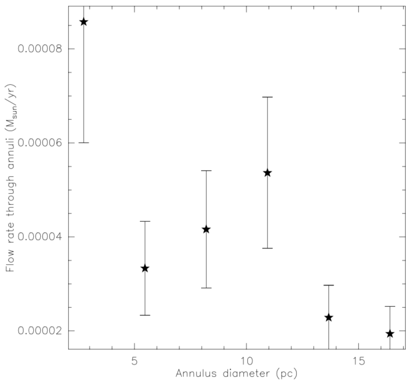
Figure 14: Estimated mass flow rate versus the distance of the chosen annulus from the cloud center (see Fig. 4). Error-bars are just approximate $\pm$30% ranges.

Employing this approach, we can estimate the mass flow rate at varying distances from the central filament. Figure 14 presents the derived $\dot{M}$ values versus the distance of the annulus from the center of the region. Being on the order of a few times $10^{-5}$ M_⊙yr^-1, these flow rates appear rather constant over the extent of the cloud. The absolute values should be considered as lower limits because of the two-dimensional projection of the velocity gradient on the plane of the sky. Interestingly, in the gravitationally driven cloud collapse simulation by Gómez & Vázquez-Semadeni (2014), an accretion rate onto the central filament of $\sim$150 M_⊙(Myr)^-1, corresponding to $1.5\times 10^{-4}$ M_⊙yr^-1, is inferred. Taken into account that our observed values should be lower limits because of projection effects, both accretion rates appear to agree within an order of magnitude. However, one should keep in mind that this comparison is based on only one cloud and one simulation, so more statistical work is needed on both sides to infer tighter constraints on the mass flow rates during cloud formation in general.

These data can be interpreted as indicative for a constant mass flow from large to small spatial scales. Such constant flow rates could, for example, occur in a self-similar gravitationally dominated collapse picture (e.g., Whitworth & Summers 1985; Li 2018).

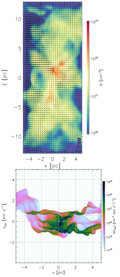
Figure 15: Simulation results corresponding to data first published in Gómez & Vázquez-Semadeni (2014). The top panel presents a column density projection of the simulations at a time step of 21.5 Myr with velocity vectors showing the gas motions on top. The bottom panel shows the corresponding position-velocity cut along the X-axis at a Y-offset of 0.1 pc. The color-coding in both plots shows the column density of the gas.

4.4 Comparison with simulations

As one possible comparison of our observational results with numerical modeling studies, we choose the molecular cloud formation simulation originally presented in Gómez & Vázquez-Semadeni (2014). They model the formation of the cloud of comparable size to G28.3 via the collision of two oppositely directed warm gas streams (Fig. 15). The collision triggers a phase transition to the cold medium, the cloud grows rapidly in mass until it becomes Jeans-unstable and then collapses. The successive contracting motions of the cloud are gravitationally driven. The initial low-density cloud setup of the simulation encompasses an area with diameter of $\sim$50 pc, and they form dense filaments of $\sim$15 pc length with masses of $\sim$600 M_⊙ above densities of $10^{3}$ cm^-3. These values agree order-of-magnitude-wise with our observed cloud and filamentary region G28.3. The collapse is simulated in the smoothed-particle hydrodynamics framework with the GADGET-2 code including self-gravity and heating and cooling functions that imply thermal bistability of the gas. For more details about the simulations, we refer to Gómez & Vázquez-Semadeni (2014).

We are focusing here on their “Filament 2”. While the paper mainly shows the images from a snapshot at 26.6 Myr of their modeled evolution, here we present a slightly younger evolutionary stage at 21.5 Myr. At this time, the filamentary cloud is still wider and the central clump less filamentary, although it is already undergoing cloud-scale gravitational contraction, accreting from the background mostly in the direction perpendicular to the filament, and along the filament onto the central hub. This can be seen in Fig. 15 (top panel), which shows a column density projection of the cloud and velocity vectors on the plane of the figure.

Even more important are the kinematics, and Figure 15 (bottom panel) shows a position-velocity perpendicular to the filamentary structure. In analogy to our observations, the simulation X-axis resembles the north-south orientation of our IRDC G28.3 data. Interestingly, at negative offsets, the gas peaks at velocities of roughly 2.5 km s^-1 whereas at positive offsets most of the gas is at around -0.5 km s^-1. It should be noted that at these positive offsets there remains still some lower column density gas left at positive velocities. While the magnitude of the velocity difference between the two sides of the cloud is smaller than in our observations, qualitatively, the position-velocity cuts of the simulations and observations resemble each other well.

Since here we are comparing only one simulation with one observational dataset, deriving general conclusions is difficult. However, the qualitative agreement between the observations and simulations indicates that the G28.3 cloud may indeed form via gravitationally driven converging gas flows.

Another, maybe more speculative aspect of these simulations is that at large scales, a phenomenon similar to the inside-out collapse operates (see Sec. 7.2 of Vázquez-Semadeni et al. 2019). That is, there seems to be an expanding infall wave, so that material further outside begins to fall in later. We speculate that this behavior could also explain the apparent decoupling of the HI from the denser molecular gas in our observational data.

4.5 Dynamical star formation

How can we interprete the various results obtained above in the framework of dynamical star formation? Synthesizing the results from the previous sections, we find:

• The dense infrared dark cloud is embedded in an extended cloud of more diffuse molecular and atomic gas. While the CNM traced by the HISA does not show any clear velocity gradient, the other three tracers ¹³CO(1–0), [CI] and ¹³CO(3–2) exhibit a velocity gradient from north to south. The HOG and velocity structure function analysis confirm this difference indicating a decoupling of the atomic CNM from the denser central cloud. This is further supported by the decrease of HISA towards the central filamentary part of the cloud.

• The position-velocity diagrams of ¹³CO(1–0), [CI] and ¹³CO(3–2) reveal two velocity components from the north and the south that converge at a velocity of $\sim$78 km s^-1 of the central infrared dark cloud. This is indicative of a converging gas flow.

• Estimates of the gas flow rate from the cloud edge to the center reveal rather constant values over all scales. This can be interpreted as a constant gas flow from the outside to the central infrared dark cloud. Such constant flow rate is consistent with a self-similar, gravitationally driven collapse of a cloud.

• Comparing the derived second order velocity structure functions with those derived from simulated molecular clouds, the data are consistent with gas flows that are dominated by the formation of hierarchical structures and cores.

Taking these results together, the spatial and kinematic signatures obtained toward the infrared dark cloud G28.3 are consistent with converging gas flows that may trigger the formation of the central IRDC and the gravitational collapse of the cloud as site of active star formation. It is difficult to clearly differentiate between colliding flows that started in the low-density medium, or a cloud-cloud collision picture where two cold dense cloud collide. Nevertheless, since cloud-cloud collisions may be considered as the high-density version of the broader picture of colliding gas flows, both pictures are consistent with a dynamic cloud and star formation scenario.

The remaining follow-up question relates to the origin of such converging gas flows? Are the flows externally triggered, e.g., due to nearby supernovae explosions or the spiral arm passage of the gas? Or are the flows produced by the large-scale cloud collapse? The constant flow rates from large to small spatial scales are consistent with a self-similar, gravitationally driven cloud collapse. Furthermore, the fact that the converging gas flow signatures are only seen in the denser gas tracers, whereas the lower-density and more external CNM as traced by HISA does not exhibit any significant velocity gradient, can be considered as additional indication for the gas flow being gravitationally driven in the dense gas region. However, with the given data, external compression as the cause of the converging flow signatures cannot be excluded. It may even be that a combination of external compression and gravitational collapse could explain the data: The external driving by a spiral arm shock or supernova compression may be the starting point of the collapse, which then may rapidly be taken over by gravity. In that picture, externally initiated converging gas flows and global gravitational collapse could be part of the same overall scenario.

5 Conclusions and Summary

The analysis of the kinematic parameters of the cloud surrounding the IRDC G28.3 reveals clear signatures of two gas flows that converge at the position of the central IRDC. The mass flow rather appears almost constant from large to small spatial scales. The spectral and spatial signatures of the HISA compared to the other tracers are consistent with a kinematic decoupling of the HISA-traced CNM from the denser gas. Overall, the analysis is in general agreement with hierarchical cloud structures that are dynamically evolving within converging gas flows. The origin of such converging flows is consistent with a self-similar, gravitationally driven collapse of the cloud. However, converging gas flows could also be caused by external drivers, e.g., spiral arm shocks or supernovae driven shocks. The differentiation of the possible different origins of the gas flows remains subject of future investigations.