Effect of Autonomous Driving on Traffic Breakdown in Mixed Traffic Flow: A Critical Mini-Review

Abstract

In this mini-review, a critical analysis of the effect of autonomous driving vehicles on traffic breakdown in mixed traffic flow consisting of randomly distributed human driving and autonomous driving vehicles is made. Autonomous vehicles based on classical (standard) adaptive cruise control (ACC) in a vehicle and on an ACC in the framework of three-phase traffic theory (TPACC – Three-traffic-Phase ACC) introduced recently [Phys. Rev. E 97 (2018) 042303] are considered. Due to the particular importance of characteristics of traffic breakdown (transition from free traffic flow to congested traffic) for almost all approaches to traffic control and management in traffic networks, the basis of this critical review is a study of the effect of autonomous vehicles on the probability of traffic breakdown and on stochastic highway capacity in mixed traffic flow. We show that within a wide range of dynamic parameters of classical ACC, the ACC-vehicles can deteriorate the traffic system considerably while initiating traffic breakdown and reducing highway capacity at a bottleneck. Contrarily, in the same range of parameters of dynamic rules of TPACC, the TPACC-vehicles either do not effect on traffic characteristics or sometimes can even improve them. To understand physical reasons for the effect of classical ACC- and TPACC-vehicles on traffic breakdown, we introduce a model of ACC that can be considered a combination of dynamic features of classical ACC and TPACC. With the use of this model, we find how the amplitude of a local speed disturbance caused by the ACC in a vicinity of a bottleneck and the probability of traffic breakdown depend on the dynamic parameters of the ACC. To emphasize that the deterioration of the characteristics of mixed traffic flow through classical ACC-vehicles is not associated with a well-known effect of string instability of platoons of autonomous vehicles, we limit by a consideration of only such classical ACC-vehicles whose platoon satisfies condition for string stability.

1 Introduction

It is commonly assumed that future vehicular traffic is a mixed traffic flow consisting of random distributed human driving and autonomous (automated) driving vehicles (see, e.g., [1, 2, 3, 4, 5, 6, 7, 8, 9, 10, 11, 12], [13, 14, 15, 16, 17, 18, 19, 20, 21, 22, 23, 24, 25]). There exist a large series of papers by the well-known and massive $``$Automated Highway System” project involving the US government and a large number of transportation researchers [17, 18], EU projects [19], and projects made in Germany [20]. A consortium of researches all over the world performed extensive and pioneering research into autonomous and automated driving vehicle systems (see references to these extensive research, for example, in reviews and books by Ioannou [1], Ioannou and Sun [2], Ioannou and Kosmatopoulos [3], Shladover [21], Rajamani [22], Meyer and Beiker [8], Bengler et al. [9], and Van Brummelen et al. [16]).

An autonomous driving vehicle is a self-driving vehicle that can move without a driver. Autonomous driving is realized through the use an automated system in a vehicle: The automated system has control over the vehicle in traffic flow. For this reason, autonomous driving vehicle is also called automated driving (or automatic driving) vehicle. It should be noted that in the engineering science the terms autonomous driving and automated driving are not synonyms. There are two reason for this. While an autonomous driving vehicle should be able to move without a driver in the vehicle, there are several different levels of automation associated with automated driving. The levels include, for example, a level of $``$conditional automation” in which the driver must be present to provide any corrections when needed and a level of $``$full automation” in which the automated vehicle system is in complete control of the vehicle and human presence is no longer needed. Additionally, in contrast with autonomous driving vehicle that moves fully autonomous from other vehicles, it is often assumed that automated driving can be supported by so-called cooperative driving that can be realized through a diverse variety of cooperative automated systems like vehicle-to-vehicle (V2V) communication (ad-hog vehicle networks) and vehicle-to-infrastructure (V2X) communication. However, to study dynamic strategies for future reliable autonomous driving that should increase network capacity and traffic safety, in this article we limit a consideration of an automated vehicle system that is in complete control of the vehicle as well as we assume that there are no cooperative vehicle systems that can support automated driving. In other words, for the subject discussed in this article there is no difference between the terms autonomous driving and automated driving.

As mentioned, autonomous driving vehicles should considerably enhance highway capacity. Highway capacity is limited by traffic breakdown at road bottlenecks. Traffic breakdown is a transition from free flow at a bottleneck to congested traffic at the bottleneck (see, e.g., reviews and books [26, 27, 28, 29, 30, 31, 32, 33, 34], [35, 36, 37, 38, 39, 40, 41, 42, 43, 44, 45, 46], [47, 48, 50, 51, 52, 53, 54, 55]). It has been found that highway capacity exhibits a stochastic nature [56, 57]: At the same flow rate in free flow at a bottleneck traffic breakdown can occur but it should not necessarily occur. In further empirical studies of this probabilistic traffic breakdown [56, 57], it has been found that empirical traffic breakdown exhibits the nucleation nature [58, 59, 60, 61, 62, 63, 64, 65, 66, 67]: Traffic breakdown can be induced by a time-limited localized congested pattern reaching a highway bottleneck. Because empirical traffic breakdown in free flow at a bottleneck is the probabilistic phenomenon that exhibits the empirical nucleation nature, the probability of traffic breakdown in free flow at the bottleneck is one of the main characteristics of the traffic stream.

As known (see, e.g., reviews and books [26, 27, 28, 34, 53, 54, 55]), most important features of traffic breakdown in free flow at an on-ramp bottleneck on a single-lane road are qualitatively the same as those in highly heterogeneous traffic flow consisting of very different types of vehicles on multi-lane road with different types of road bottlenecks. In particular, this conclusion is related to the empirical flow-rate dependence of the breakdown probability [34, 55]. Therefore, to find the effect of different features of the dynamics of autonomous driving vehicles in mixed traffic flow on the probability of traffic breakdown at a road bottleneck, it is sufficient to study a simple case of mixed vehicular traffic where traffic consists only of two types of vehicles (human driving and autonomous driving vehicles) moving on a single-lane road with an on-ramp bottleneck.

On the single-lane road, no vehicles can pass. For this reason, the effect of autonomous driving on traffic breakdown and highway capacity can be understood through an analysis of an adaptive cruise control (ACC) in a vehicle: An ACC-vehicle follows the preceding vehicle (that can be either a human driving vehicle or an ACC-vehicle) automatically based on some ACC dynamics rules of motion (see, e.g., [1, 2, 3, 4, 5, 6, 7, 11, 12, 22, 23, 24]).

In [68, 69, 70, 71] the author introduced a strategy of ACC in the framework of the three-phase theory called TPACC – Three-traffic-Phase ACC (for a review, see [72, 73, 74]). One of the most important features of TPACC is the existence of the indifference zone in car-following of the three-phase theory. In this review article, we the use of a simple TPACC model [73, 74] we will show that the TPACC strategy can exhibit the following important advantages in comparison with the classical (standard) ACC strategy:

(i) The mean amplitude of speed disturbances at a road bottleneck occurring through TPACC-vehicle can be considerably smaller than that introduced by classical ACC-vehicles at the same model parameters.

(ii) In mixed traffic flow with TPACC-vehicles the probability of traffic breakdown at a road bottleneck can be considerably smaller than in mixed traffic flow with classical ACC-vehicles.

We explain the physics of the improving of the traffic stream through TPACC-vehicles.

The main objective of this review paper is a critical comparison between autonomous vehicles based on classical ACC and on TPACC. Characteristics of traffic breakdown and stochastic highway capacity are particular important for almost all approaches to traffic control and management in traffic networks. For this reason, the critical comparison between different dynamical characteristics of autonomous vehicles is based on a study of the effect of autonomous vehicles on the probability of traffic breakdown and on stochastic highway capacity in mixed traffic flow consisting of randomly distributed human driving and autonomous driving vehicles.

To make this critical analysis clear, in this review paper we introduce a model of ACC that can be considered a combination of dynamic features of classical ACC and TPACC. With the use of this model, we find how the amplitude of a local speed disturbance caused by the ACC in a vicinity of a bottleneck and the probability of traffic breakdown depend on the dynamic parameters of the ACC. To emphasize that the deterioration of the characteristics of mixed traffic flow through classical ACC-vehicles is not associated with a well-known effect of string instability of platoons of autonomous vehicles, we limit by a consideration of only such classical ACC-vehicles whose platoon satisfies condition for string stability.

The article is organized as follows: First, we discuss the empirical nucleation nature of traffic breakdown and associated stochastic highway capacity as well as the consequences the empirical nucleation nature of traffic breakdown for the evaluation of performance of autonomous driving in mixed traffic flow through the use of traffic simulations (Sec. 2). In this section we will also consider the reason for the failure of standard approaches for simulations of mixed traffic flow. Classical (standard) ACC strategy is the subject of Sec. 3. The strategy to autonomous driving in the framework of the three-phase theory called TPACC is discussed in Sec. 4. The effect of classical ACC and TPACC on traffic breakdown at a bottleneck is studied in Sec. 5. The dependence of characteristics of traffic breakdown on time headway of classical ACC and TPACC is the subject of Sec. 6. The influence of dynamic rules of autonomous driving on speed disturbances at the bottleneck is considered in Sec.7. The effect of platoons of autonomous driving vehicles on the probability of traffic breakdown in mixed traffic flow is discussed in Sec. 8. Traffic stream flow characteristics of mixed traffic flow are discussed in Sec. 9. In discussion (Sec. 10), we formulate paper conclusions (Sec. 10.1), consider the applicability of the TPACC model for a reliable analysis of some features of future autonomous driving in mixed traffic flow (Sec. 10.2) and discuss a question whether vehicular traffic in networks consisting of only autonomous vehicles is real option in the future (Sec. 10.3). In Appendix A, we present the Kerner-Klenov stochastic microscopic three-phase model for human driving vehicles [75, 76, 77] used for all simulations of mixed traffic flow made in the paper, in Appendix B we explain simulations of the classical ACC model, in Appendix C we consider a discrete TPACC model used for simulations of TPACC model, in Appendix D we present a discrete version of a ACC-model that can be considered a combination of the classical ACC- and TPACC-models, in Appendix E we consider a model of vehicle merging at an on-ramp bottleneck, and in Appendix F we consider boundary conditions used for simulations of mixed traffic flow.

2 Nucleation Nature of Traffic Breakdown and Its Consequences for Evaluation of Performance of Autonomous Driving in Mixed Traffic Flow

2.1 Three-Phase Traffic Theory

Three-phase traffic theory is a framework for understanding of states of empirical traffic flow in three traffic phases [53, 55, 58, 59, 60, 61, 62, 63, 64, 65, 66]:

1. Free flow (F).

2. Synchronized flow (S).

3. Wide-moving jam (J).

The synchronized flow and wide-moving jam traffic phases belong to congested traffic.

The synchronized flow and wide moving jam phases in congested traffic are defined through the use of the following macroscopic empirical criteria [J] and [S] for, respectively, the wide-moving jam and the synchronized flow traffic phases in congested traffic [53, 54, 55, 78, 79, 80, 81, 82, 83]:

• [J] The wide moving jam phase is defined as follows. A wide moving jam is a moving jam that maintains the mean velocity of the downstream front of the jam as the jam propagates. Vehicles accelerate within the downstream jam front from low speed states (sometimes as low as zero) inside the jam to higher speeds downstream of the jam. A wide moving jam maintains the mean velocity of the downstream jam front, even as it propagates through other different (possibly very complex) traffic states of free flow and synchronized flow or highway bottlenecks. This is a characteristic feature of the wide moving jam phase.

• [S] The synchronized flow phase is defined as follows. In contrast to the wide moving jam traffic phase, the downstream front of the synchronized flow phase does not maintain the mean velocity of the downstream front. In particular, the downstream front of synchronized flow is often fixed at a bottleneck. In other words, the synchronized flow traffic phase does not show the characteristic feature [J] of the wide moving jam phase.

• The phase definitions [S] and [J] mean that if in a set of empirical traffic data congested traffic states associated with the wide moving jam traffic phase have been identified through the use of the criterion [J], then with certainty all remaining congested states in the empirical data set are related to the synchronized flow phase.

The downstream front of synchronized flow separates synchronized flow upstream from free flow downstream. Within the downstream front of synchronized flow vehicles accelerate from lower speeds in synchronized flow upstream of the front to higher speeds in free flow downstream of the front.

2.2 Empirical Nucleation Nature of Traffic Breakdown

In all empirical data measured over years in different countries, traffic breakdown at a highway bottleneck is a phase transition from free flow (F) to the synchronized flow phase (S) of congested traffic (F$\rightarrow$S transition). Therefore, traffic breakdown at a highway bottleneck and an F$\rightarrow$S transition at the bottleneck are synonyms.

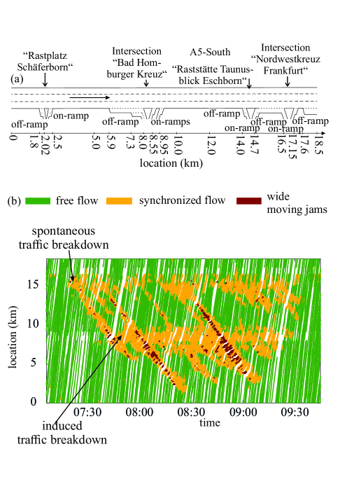
Figure 1: (Color online) Empirical spontaneous and empirical induced traffic breakdown (F$\rightarrow$S transition) with complex pattern formations in probe vehicle data: (a) Schema of highway section; there are two bottlenecks at which traffic breakdown is observed (explanations of these bottlenecks can be found in Secs. 2.3.2 and 9.2.1 of [53]): (i) A downstream bottleneck caused by an off-ramp within an intersection $``$Nordwestkreuz Frankfurt” (effective bottleneck location at about 15 km); (ii) an upstream bottleneck caused by on-ramps within at an intersection $``$Bad Homburger Kreuz” (effective bottleneck location at about 9 km). (b) Overview of phase transitions with pattern formation; green, yellow, and red parts on trajectories in (b) are related to the free flow, synchronized flow, and wide moving jam traffic phases. To distinguish between the three traffic phases, a model for the detection of phase transition points along a vehicle trajectory of Ref. [87] has been applied; parameters of the model, in which some speed and time thresholds for the different traffic phases have been used, are related to Table 2 of Ref. [87]. Adapted from [88].

Probably the most important empirical feature of the synchronized flow is that the F$\rightarrow$S transition (traffic breakdown) exhibits the nucleation nature [58, 59, 60, 61][62, 63, 64, 65, 66]. This means that traffic breakdown occurs in a metastable free flow with respect to an F$\rightarrow$S transition at the bottleneck. Indeed, empirical data shows that empirical traffic breakdown (F$\rightarrow$S transition) at a highway bottleneck can be either spontaneous or induced traffic breakdown.

• As shown and proven in [53, 54, 55, 67], the occurrence of empirical induced traffic breakdown at the bottleneck is the empirical proof of the empirical nucleation nature of traffic breakdown (F$\rightarrow$S transition).

An empirical example of both spontaneous and induced traffic breakdowns occurring at different bottlenecks is shown in Fig. 1.

2.3 Explanation of Traffic Breakdown Nucleation in Three-Phase Traffic Theory

The main reason of the three-phase theory is the explanation of the empirical nucleation nature of traffic breakdown (F$\rightarrow$S transition) at the bottleneck. To reach this goal, in congested traffic a new traffic phase called synchronized flow has been introduced [53, 54, 55, 78, 79, 80, 81, 82, 83]. The basic feature of the synchronized flow traffic phase formulated in the three-phase theory leads to the nucleation nature of the F$\rightarrow$S transition. In this sense, the synchronized flow traffic phase, which ensures the nucleation nature of the F$\rightarrow$S transition at a highway bottleneck, and the three-phase traffic theory can be considered synonymous.

In the three-phase traffic theory, the empirical nucleation nature of traffic breakdown is associated with the metastability of free flow with respect to traffic breakdown (F$\rightarrow$S transition) at a highway bottleneck. The metastability of free flow with respect to traffic breakdown (F$\rightarrow$S transition) is as follows [53, 55, 58, 59, 60, 61, 62, 63, 64, 65, 66, 67]: There can be many speed (density, flow rate) disturbances in free flow at the bottleneck. Amplitudes of the disturbances can be very different. When a disturbance occurs randomly whose amplitude is larger than a critical one, then traffic breakdown occurs. Such a disturbance resulting in traffic breakdown is called nucleus for the breakdown. Otherwise, if the disturbance amplitude is smaller than the critical one, the disturbance decays. As a result, no traffic breakdown occurs.

As emphasized in [55, 78, 79, 80, 81, 82, 83], the metastability of free flow with respect to traffic breakdown (F$\rightarrow$S transition) at a highway bottleneck has no sense for standard traffic and transportation theories. Reviews of the standard traffic and transportation theories can be found in [26, 27, 28, 29, 30, 31, 32, 33], [34, 35, 36, 37, 38, 39, 40, 41, 42, 43, 44], [45, 46, 47, 48, 50, 51, 52, 90, 91]. The criticism of the standard traffic and transportation theories has been made in reviews and books [53, 54, 55, 78, 79, 80, 81, 82, 83]. In particular, in [55, 78, 79, 80], [81, 82, 83] it has been shown that the three-phase theory is incommensurable with all earlier traffic flow theories and models. The term $``$incommensurable” has been introduced by Kuhn [92] to explain a paradigm shift in a scientific field.

2.4 Understanding Stochastic Highway Capacity

One of the most important consequences of the empirical nucleation nature of traffic breakdown at a highway bottleneck is as follows [53, 55]: The metastability of free flow with respect to traffic breakdown (F$\rightarrow$S transition) is realized within a flow rate range (Fig. 2)

$$C_{\rm min}\leq q_{\rm sum}<C_{\rm max},$$ (1)

where $q_{\rm sum}$ is the flow rate in free flow at a highway bottleneck, $C_{\rm min}$ is a minimum highway capacity, $C_{\rm max}$ is a maximum highway capacity.

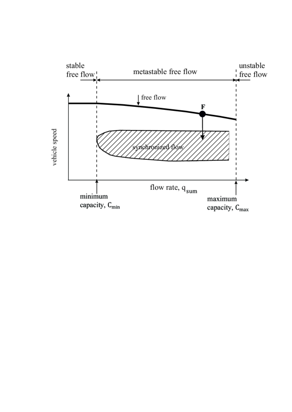
Figure 2: Qualitative explanation of the empirical metastability of free flow with respect to traffic breakdown (F$\rightarrow$S transition) at bottleneck in three-phase theory [53, 55, 58, 59, 60, 61, 62, 63, 64, 65, 66]. Qualitative Z-speed–flow-rate characteristic for traffic breakdown; F – free flow, S – synchronized flow (two-dimensional (2D) hatched region). Arrow F$\rightarrow$S illustrates symbolically one of possible F$\rightarrow$S transitions occurring in a metastable state of free flow when a nucleus appears in the free flow at the bottleneck. Adapted from [55].

This conclusion of empirical observations of traffic breakdown (F$\rightarrow$S transition) at the bottleneck leads to the following definition of stochastic highway capacity of free flow at a highway bottleneck made in the three-phase theory [53]:

• At any time instant, there are the infinite number of highway capacities $C$ of free flow at the bottleneck. The range of the infinite number of highway capacities is limited by the minimum highway capacity $C_{\rm min}$ and the maximum highway capacity $C_{\rm max}$ (Fig. 2):

  $$C_{\rm min}\leq C\leq C_{\rm max},$$ (2)

  where $C_{\rm min}<C_{\rm max}$. The existence of an infinite number of highway capacities at any time instant means that highway capacity is stochastic.

The physical sense of this capacity definition is as follows. Highway capacity is limited by traffic breakdown (F$\rightarrow$S transition) in an initial free flow at a highway bottleneck. In other words, any flow rate $q_{\rm sum}$ in free flow at the bottleneck at which traffic breakdown can occur is highway capacity. At any time instant, there are the infinite number of such highway capacities $C=q_{\rm sum}$ at which traffic breakdown can occur. These capacities satisfy conditions (2). Thus, in the three-phase theory any flow rate $q_{\rm sum}$ in free flow at a highway bottleneck that satisfies conditions

$$C_{\rm min}\leq q_{\rm sum}\leq C_{\rm max}$$ (3)

is equal to one of the stochastic highway capacities of free flow at the bottleneck (Fig. 2). A more detailed consideration of the nucleation nature of traffic breakdown and stochastic (probabilistic) features of the infinite number of the highway capacities can be found in [55, 79, 80].

2.5 Paradigm Shift in Traffic and Transportation Science

The fundamental change in the meaning of stochastic highway capacity made in the three-phase traffic theory can be considered the paradigm shift in traffic and transportation science. This is because the meaning of highway capacity is the basis for the development of methods for traffic control, management, and organization of a traffic network as well as ITS-applications.

The paradigm of standard traffic and transportation theories can be formulated as follows: At a given time instant there is a value of highway capacity. This is also true when it is assumed that at any time instant there is a stochastic value of highway capacity. This means that when the flow rate at a bottleneck exceeds the capacity value at this time instant, traffic breakdown must occur at the bottleneck. This classical understanding of highway capacity is the basis for standard methods for traffic control, management, and organization of a traffic network as well as ITS-applications (see results of standard traffic and transportation theories as well as some results of their ITS-applications, for example, in reviews and books [26, 27, 28, 29, 30, 31, 32, 33, 34, 35, 36, 37, 38], [39, 40, 41, 42, 43, 44, 45, 46], [47, 48, 49, 50, 51, 52], [90, 91, 93, 94, 95, 96, 97, 98, 99, 100, 101], [102, 103, 104, 105, 106, 107, 108, 109, 110, 111], [112, 113, 114, 115, 116, 117, 118]).

In accordance with the understanding of stochastic highway capacity made in the three-phase traffic theory [53, 55, 58, 59, 60, 61, 62, 63, 64, 65, 66] and briefly reviewed in Sec. 2.4, the new paradigm in traffic and transportation science can been formulated as follows:

• At any time instant there is a range of the flow rate (1) within which traffic breakdown at the bottleneck can occur with some probability but traffic breakdown does not necessarily occur (Fig. 2).

Thus, in contrast with the standard traffic theories, in the three-phase traffic theory there is a range of highway capacity values between a minimum and a maximum highway capacity at any time instant (Fig. 2). When the flow rate at a bottleneck is inside this capacity range related to this time instant, traffic breakdown can occur at the bottleneck only with some probability, i.e., in some cases traffic breakdown occurs, in other cases traffic breakdown does not occur. The existence at any time instant of the infinite number of highway capacity values within the capacity range means that highway capacity is stochastic. Both the minimum and maximum highway capacities are also stochastic values. We can make the following conclusions:

• This basic change in the meaning of stochastic highway capacity results from the empirical nucleation nature of traffic breakdown at a bottleneck.

• Three-phase traffic theory is a theoretical framework that explains stochastic highway capacity by a capacity range that exists at any time instant. When at a time instant the flow rate at the bottleneck is inside the capacity range related to this time instant, traffic breakdown can occur with some probability but traffic breakdown does not necessarily occur.

To be consistent with the empirical nucleation nature of traffic breakdown, other methods (in comparison with the methods developed in accordance with the standard meaning of highway capacity) for traffic control and management in traffic networks, other models for simulations of mixed traffic flow as well as other models for the evaluation of ITS-applications should be developed.

2.6 Driver Behavioral Assumption of Traffic Breakdown Nucleation in Three-Phase Traffic Theory

To answer a question about a driver behavior that is responsible for the empirical nucleation nature of traffic breakdown (F$\rightarrow$S transition) at a highway bottleneck, we should mention that when a driver approaches a slower moving preceding vehicle and the driver cannot immediately pass the slow vehicle, the driver must decelerate to the speed of the slow moving preceding vehicle. This driver deceleration can be called driver speed adaptation (Fig. 3 (a)). To escape from this car-following of the slow moving preceding vehicle, the driver searches for the opportunity to accelerate. We call vehicle acceleration from the car-following of the slow moving preceding vehicle as over-acceleration.

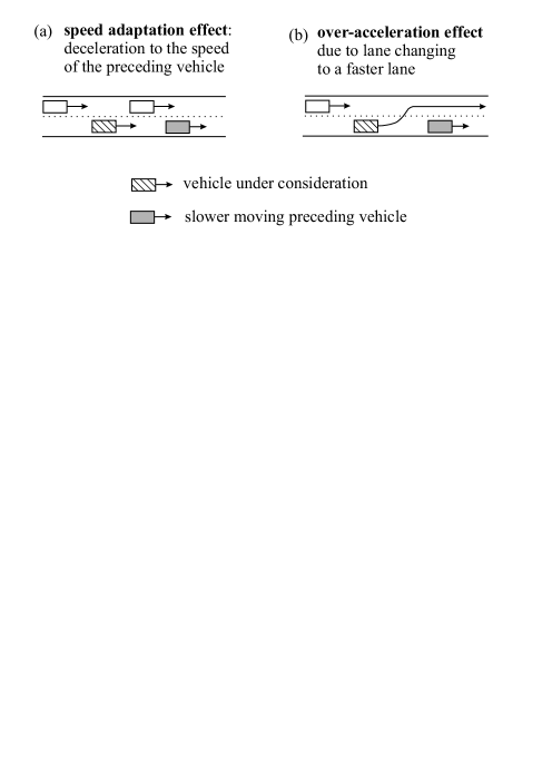
Figure 3: Qualitative explanation of driver speed adaptation (a) and driver over-acceleration through the lane changing (b).

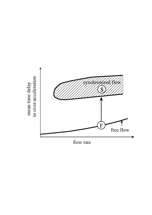
Figure 4: Hypothesis of three-phase traffic theory about the discontinuous character of the mean time delay in over-acceleration. F is a state of free flow, S is a state of synchronized flow.

To simplify a qualitative explanation of over-acceleration, we consider a vehicle approaching a slow preceding vehicle moving in the right line of a multi-lane road. If the vehicle under consideration cannot immediately pass the slow moving vehicle, the vehicle must decelerate to a lower speed of the preceding vehicle ($``$speed adaptation” in Fig. 3 (a)). On the multi-lane road, over-acceleration leading to the vehicle escaping from the car-following is often possible through lane changing to a faster lane with the subsequent passing of the slow moving vehicle (Fig. 3 (b)). However, after the driver has begun the speed adaptation to the speed of the slow moving preceding vehicle (Fig. 3 (a)) there can be a waiting time before the lane changing maneuver leading to vehicle acceleration with the subsequent passing of the slow moving vehicle is successful. We call this waiting time as a time delay in over-acceleration.

The vehicle density in synchronized flow is larger than the density is in free flow at the same flow rate. We can assume that the larger the vehicle density, the more difficult to escape from the car-following of the slow moving preceding vehicle through over-acceleration. Respectively, the larger the vehicle density, the longer should be the mean time delay in over-acceleration. Through a large synchronized flow density, vehicles prevent each other to accelerate to a higher speed. Such a strong bunching of vehicle motion distinguishes synchronized flow from free flow: In free flow, vehicle bunching is weak and, therefore, vehicles can much easier escape from the car-following of the slow moving preceding vehicle. This qualitative consideration leads to the assumption made in the three-phase traffic theory about the discontinuous character of the mean time delay in over-acceleration (Fig. 4): In synchronized flow, the mean time delay in over-acceleration should be considerably longer than it is in free flow.

Therefore, during traffic breakdown (F$\rightarrow$S transition) at a bottleneck there should be a jump in the mean time delay in over-acceleration from a relatively short mean time delay in over-acceleration in free flow to a considerably longer mean time delay in over-acceleration in synchronized flow (up-arrow in the mean time delay in over-acceleration in Fig. 4). The assumption about the discontinuous character of the the mean time delay in over-acceleration (Fig. 4) is consequent with the discontinuous character of the speed–flow-rate dependence (Fig. 2).

The hypothesis about the discontinuous character of the mean time delay in over-acceleration (Fig. 4) is equivalent to the hypothesis about the discontinuous character of the probability that over-acceleration is realized during a given time interval (probability of over-acceleration for short) (Fig. 5) [53, 54, 55]. Indeed, the probability of over-acceleration is the larger, the shorter the mean time delay in over-acceleration (Fig. 4). Therefore, traffic breakdown (F$\rightarrow$S transition) at the bottleneck that leads to a jump in the mean time delay in over-acceleration (up-arrow in Fig. 4) is also accompanied by a drop in the probability of over-acceleration (down-arrow in Fig. 5).

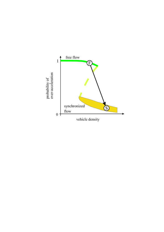
Figure 5: Hypothesis of three-phase traffic theory about the discontinuous character of the probability of over-acceleration. F is a state of free flow, S is a state of synchronized flow. Down-arrow shows qualitatively a drop in the probability of over-acceleration caused by traffic breakdown (F$\rightarrow$S transition) at a bottleneck.

It should be emphasized that the time delay in over-acceleration should not be confounded with the well-known driver reaction time. Indeed, for a safety lane changing a driver should wait for the occurrence of a long enough (safety) time headway between two following each other vehicles in the neighborhood lane to which the driver would like to change. Time headway between vehicles in the neighborhood lane do not depend on the reaction time of the driver that wants to change to this lane. However, the waiting time for the safety lane changing depends on time headway between vehicles in the neighborhood faster lane. In turn, this waiting time is the time delay in over-acceleration through lane changing to a faster lane (Fig. 3 (b)).

• Thus, we can conclude that even if the driver reaction time were negligible short, the mean time delay in over-acceleration is a finite value that exhibits the discontinuous character qualitatively shown in Fig. 4.

We can also assume that the discontinuous behavior of the mean time delay in over-acceleration through lane changing to a faster lane shown in Fig. 4 can remain for autonomous driving vehicles, for which (in contrast to human driving vehicles) the reaction time on an unexpected deceleration of the preceding vehicle or on a sudden reduction in the spacing due to a merging vehicle can theoretically be made as short as zero. Indeed, as for human driving vehicles rather than the reaction time of an autonomous driving vehicle, values of time headway between vehicles in the neighborhood faster lane determine the time delay in over-acceleration for the safety lane changing of the autonomous driving vehicle ($``$vehicle under consideration” in Fig. 3 (b)).

2.7 Main Prediction of Three-Phase Traffic Theory

The main prediction of the three-phase traffic theory is as follows.

• There is an S$\rightarrow$F instability in synchronized flow. The S$\rightarrow$F instability is a growing wave of a local increase in the speed in synchronized flow. The uninterrupted growth of this wave leads to a transition from synchronized flow to free flow. The S$\rightarrow$F instability exhibits the nucleation nature: Only a large enough initial local increase in the speed in synchronized flow can lead to the S$\rightarrow$F instability, whereas local disturbances of small enough local speed increase in synchronized flow decay.

• The nucleation nature of the S$\rightarrow$F instability governs the metastability of free flow with respect to the F$\rightarrow$S transition at the bottleneck. In its turn, the metastability of free flow with respect to the F$\rightarrow$S transition at the bottleneck explains the empirical nucleation nature of traffic breakdown [53, 89].

To explain the main prediction of the three-phase theory, we assume that traffic breakdown (F$\rightarrow$S transition) has occurred at a highway bottleneck. Due to this traffic breakdown, synchronized flow emerges at the bottleneck. We assume that the downstream front of the synchronized flow is fixed at the bottleneck. In the synchronized flow, many local speed disturbances with very different disturbance amplitudes can occur.

In the three-phase theory it has been proven that due to a finite time delay in over-acceleration discussed in Sec. 2.6, a local speed increase within one of the local speed disturbances in synchronized flow can randomly begin to grow over time. As a result, a growing wave of a local speed increase in synchronized flow appears. The development of such a traffic flow instability leads to the returning of free flow at the bottleneck. This instability is called as an S$\rightarrow$F instability [89].

Within a speed wave of a local increase in the speed of synchronized flow, there is a spatiotemporal competition between over-acceleration and speed adaptation. It has been found that a growing wave of a local speed increase in synchronized flow (S$\rightarrow$F instability) is realized only when within the speed wave over-acceleration overcomes speed adaptation. This can only be possible when the amplitude of a local speed increase in synchronized flow is large enough. In contrast, when the amplitude of a local speed increase in synchronized flow is small enough, a dissolving wave of a local increase in the speed in synchronized flow is realized. In other words, the S$\rightarrow$F instability exhibits the nucleation nature.

It must be emphasized that the S$\rightarrow$F instability [55, 89] should not be confounded with the well-known classical traffic flow instability introduced in 1950s–1960s [119, 120, 121, 122, 123, 124, 125, 126] and incorporated in a huge number of traffic flow models (see, e.g., explanations of classical traffic flow instability and references in reviews and books [29, 30, 31, 32, 33, 34, 36, 37], [40, 43, 45, 46, 47], [51, 52, 90, 91]). Indeed, the classical traffic flow instability leads to a growing wave of a local decrease in the speed in traffic flow (see, e.g., [29, 30, 31, 32, 33, 34, 36, 37], [40, 43, 45, 46, 47], [51, 52, 90, 91], [119, 120, 121, 122, 123, 124, 125, 126, 127]). In contrast with the classical traffic flow instability, the S$\rightarrow$F instability introduced in the three-phase traffic theory [55, 89] leads to a growing wave of a local increase in the speed in synchronized flow.

2.8 Failure of Standard Approaches for Simulations of Mixed Traffic Flow

It should be mentioned that the effect of autonomous (automated) vehicles on mixed traffic flow was intensively considered already in 1990s-2000s in the works by Dharba and Rajagopal [129], Marsden et al. [130], VanderWerf et al. [131, 132], Treiber and Helbing [133], Li et al. [134], Kukuchi et al. [135], Bose and Ioannou [136], Suzuki [137], Davis [23], Zhou and Peng [138], van Arem et al. [139], Kesting et al. [140, 141, 142]; this is a subject of intensive studies up to now (see, e.g., [24, 45, 143, 144, 145, 146, 147, 148], [149, 150, 151, 152, 153, 154], [155, 156, 157, 158, 159], [160, 161, 162, 163, 164, 165], [166, 167, 168, 169, 170, 171, 172] and references there).

As proven in details in the books [53, 54, 55], classical (standard) traffic flow theories and models of human driving vehicles cannot explain the empirical nucleation nature of traffic breakdown (F$\rightarrow$S transition) at the bottleneck.

• Traffic and transportation theories, which are not consistent with the nucleation nature of traffic breakdown (F$\rightarrow$S transition) at highway bottlenecks, cannot be applied for the development of reliable traffic control, dynamic traffic assignment as well as other reliable ITS-applications in traffic and transportation networks.

This criticism on all standard traffic flow models has been explained in details in the book [55]; a brief explanation of this critical statement can also be found in [79, 81, 82, 83].

In almost all studies of mixed traffic flow that the author knows models of human driving vehicles have been used that cannot explain the nucleation nature of traffic breakdown (F$\rightarrow$S transition) at the bottleneck. This criticism is also related to traffic flow theories and models used for studies of human driving vehicles in mixed traffic flow in Refs. [45, 129, 130, 131, 132, 133, 134, 135, 136], [137, 138, 139, 140, 141, 142, 143, 144, 145, 146], [147, 148, 149, 150, 151, 152, 153, 154, 155, 156], [157, 158, 159, 160, 161, 162, 163, 164], [165, 166, 167, 168, 169, 170, 171, 172]. Because the standard traffic flow theories and models contradict the empirical nucleation nature of traffic breakdown (F$\rightarrow$S transition), we can made the following conclusion.

• Applications of standard traffic flow theories and models of human driving vehicles used, for example, in the studies of mixed traffic flow in [45, 129, 130, 131, 132, 133, 134, 135, 136], [137, 138, 139, 140, 141, 142, 143, 144, 145, 146], [147, 148, 149, 150, 151, 152, 153, 154, 155, 156], [157, 158, 159, 160, 161, 162, 163, 164], [165, 166, 167, 168, 169, 170, 171, 172] lead to invalid conclusions about the effect of autonomous driving vehicles on highway capacity and traffic breakdown in mixed traffic flow.

For this reason, in this review article we will not consider results of [45, 129, 130, 131, 132, 133, 134, 135, 136], [137, 138, 139, 140, 141, 142, 143, 144, 145, 146], [147, 148, 149, 150, 151, 152, 153, 154, 155, 156], [157, 158, 159, 160, 161, 162, 163, 164], [165, 166, 167, 168, 169, 170, 171, 172] as well as results of all other simulations in which standard traffic flow models for the description of human driving vehicles in mixed traffic flow have been used, which are not consistent with the empirical nucleation nature of traffic breakdown (F$\rightarrow$S transition) at a highway bottleneck.

3 Classical (Standard) Strategy of Adaptive Cruise Control (ACC)

In a classical (standard) ACC model, acceleration (deceleration) $a^{\rm(ACC)}$ of the ACC vehicle is determined by the space gap to the preceding vehicle $g$ and the relative speed $\Delta v=v_{\ell}-v$ measured by the ACC vehicle as well as by a desired time headway $\tau^{\rm(ACC)}_{\rm d}$ of the ACC-vehicle to the preceding vehicle (see, e.g., [4, 5, 6, 7, 11, 12, 22, 23, 24]):

$$a^{\rm(ACC)}=K_{1}(g-v\tau^{\rm(ACC)}_{\rm d})+K_{2}(v_{\ell}-v),$$ (4)

where $v$ is the speed of the ACC-vehicle, $v_{\ell}$ is the speed of the preceding vehicle; here and below $v$, $v_{\ell}$, and $g$ are time-functions; $K_{1}$ and $K_{2}$ are coefficients of ACC adaptation.

It is well-known that there can be string instability of a long enough platoon of ACC-vehicles (4) [4, 5, 6, 7, 11, 12, 22, 23, 24]. As found by Liang and Peng [6], the string instability occurs under condition $K_{2}<(2-K_{1}(\tau^{\rm(ACC)}_{\rm d})^{2})/2\tau^{\rm(ACC)}_{\rm d}$: If a local speed (or time headway) disturbance appears in the platoon of ACC-vehicles, the disturbance begins to grow in its amplitude. The growth of the disturbance destroys the steadily ACC-vehicle motion in a long enough platoon of ACC-vehicles. Coefficients $K_{2}$ and $K_{1}$ of classical ACC (4) can be chosen to satisfy condition for string stability

$$K_{2}>(2-K_{1}(\tau^{\rm(ACC)}_{\rm d})^{2})/2\tau^{\rm(ACC)}_{\rm d}.$$ (5)

Under condition (5), any small local speed (or time headway) disturbance that appears in the platoon decays over time. Therefore, ACC-vehicles in the platoon remain to move at a time-independent speed at the desired time headway $\tau^{\rm(ACC)}_{\rm d})$ to each other. In this review article, we consider only ACC-vehicles whose parameters satisfy condition (5) for string stability.

It should be noted that in the works devoted to analysis of the effect of autonomous driving on traffic flow [45, 129, 130, 131, 132, 133, 134], [135, 136, 137, 138, 139, 140, 141, 142, 143], [144, 145, 146, 147], [148, 149, 150, 151, 152, 153, 156] traffic flow models for human driving vehicles have been used in which at a given time-independent vehicle speed there is a single model solution for a space gap to the preceding vehicle. Therefore, for such hypothetical steady state model solutions, there is a one-dimensional (1D) relationship between a chosen speed and the related desired (or optimal) space gap to the preceding vehicle. This well-known assumption for traffic flow models of human driving vehicles used, e.g., in [45, 129, 130, 131, 132, 133, 134], [135, 136, 137, 138, 139, 140, 141, 142, 143], [144, 145, 146, 147], [148, 149, 150, 151, 152, 153, 156] is qualitatively the same as the existence of a desired time headway $\tau^{\rm(ACC)}_{\rm d}$ of the ACC-vehicle to the preceding vehicle: For the classical ACC-rule (4) that satisfies condition for string stability (5), at a given ACC speed $v$ there is a single operating point for a desired space gap (Fig. 6)

$$g^{\rm(ACC)}=v\tau^{\rm(ACC)}_{\rm d}.$$ (6)

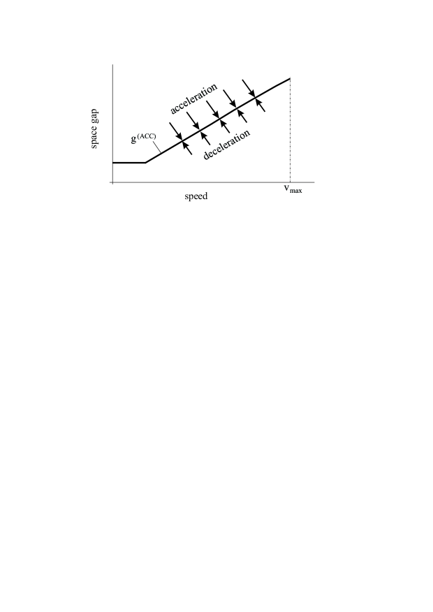
Figure 6: Operating points of the classical model of ACC (4) under condition of string stability (5): Qualitative speed dependence of desired space gap $g^{\rm(ACC)}=v\tau^{\rm(ACC)}_{\rm d}$ (6) (see, e.g., [4, 5, 6, 7, 11, 12, 22, 23, 24]).

4 ACC in Framework of Three-Phase Theory (TPACC)

4.1 Indifferent Zone in Car-Following in Three-Phase Traffic Theory

A study of real field traffic data [58, 59, 60, 61, 62, 63, 64, 65, 66, 173, 174] shows that the existence of a desired time headway $\tau^{\rm(ACC)}_{\rm d}$ of the ACC-vehicle to the preceding vehicle is inconsistent with a basic behavior of real drivers in car-following: Empirical data shows that real drivers do not try to reach a fixed time headway to the preceding vehicle in car-following.

To explain this empirical fact, the author has introduced a hypothesis about the existence of a two-dimensional (2D) region of synchronized flow states [58, 59, 60, 61, 62]: In the three-phase theory, it is assumed that when a driver approaches a slower moving preceding vehicle and the driver cannot pass it, the driver decelerates within a synchronization space gap $G$. This speed adaptation to the speed of the preceding vehicle occurs without caring what the precise space gap $g$ to the preceding vehicle is as long as it is not smaller than a safe space gap $g_{\rm safe}$ [58, 59, 60, 61, 62]. The speed adaptation occurring within the synchronization space gap $G$ leads to a 2D-region of synchronized flow states (dashed region in Fig. 7) determined by conditions

$$g_{\rm safe}\leq g\leq G.$$ (7)

The 2D-region of synchronized flow states (dashed region in Fig. 7) can also be considered $``$indifference zone” in car-following.

Accordingly to (7), a driver does not try to reach a particular (desired or optimal) time headway to the preceding vehicle, but adapts the speed while keeping time headway $\tau^{\rm(net)}=g/v$ in a range $\tau_{\rm safe}\leq\tau^{\rm(net)}\leq\tau_{\rm G}$, where $\tau_{\rm G}=G/v$, $\tau_{\rm G}$ is a synchronization time headway, $\tau_{\rm safe}=g_{\rm safe}/v$ is a safe time headway and it is assumed that the speed $v>0$.

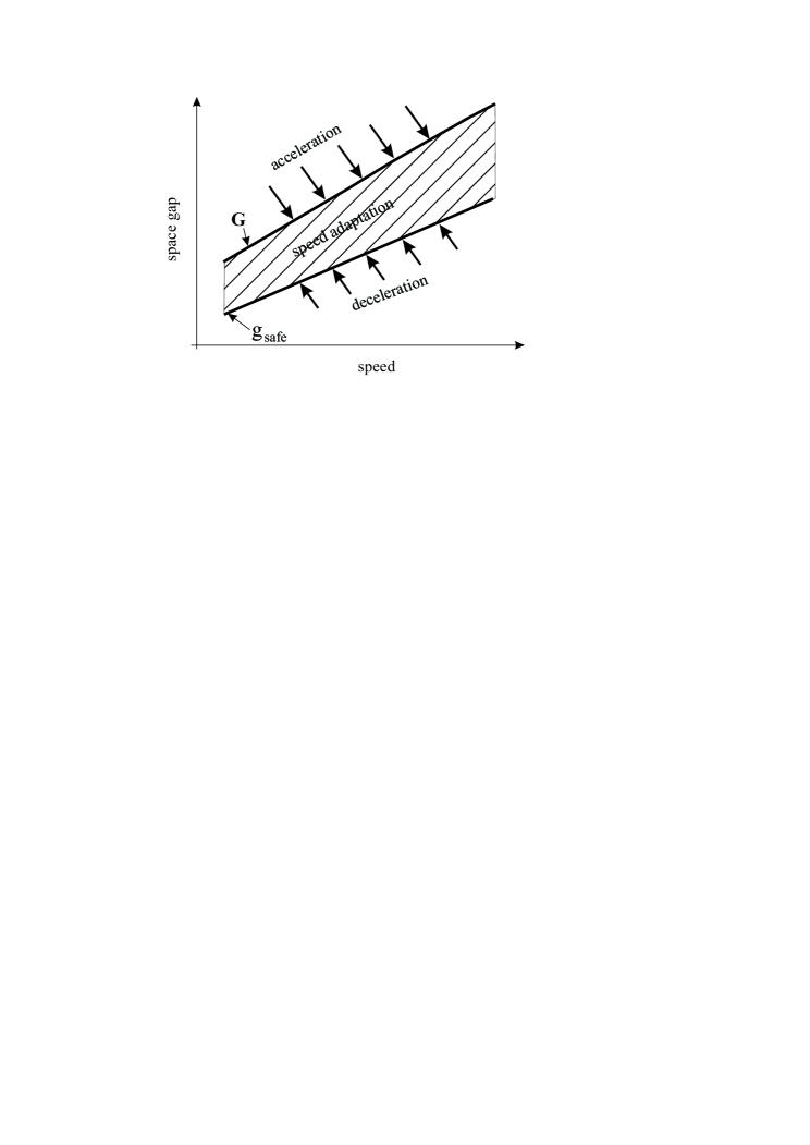
Figure 7: Qualitative explanation of indifference zone in car-following for TPACC. Qualitative presentation of a part of 2D-region for operating points of TPACC in the space-gap–speed plane: At a given speed of TPACC-vehicle there are the infinity of operating points of TPACC [68, 69, 70, 71]. $G$ is a synchronization space gap, $g_{\rm safe}$ is a safe space gap.

In [73], we have defined $``$autonomous driving in the framework of three-phase traffic theory” (TPACC) as follows:

• An autonomous driving in the framework of the three-phase traffic theory is the autonomous driving for which there is no fixed time headway to the preceding vehicle.

In inventions [68, 69, 70, 71], we have assumed that to satisfy these empirical features of real traffic, at least at some driving conditions in car-following acceleration (deceleration) of autonomous driving in the framework of the three-phase theory (TPACC) should be given by formula [68, 69, 70, 71]

$$a^{\rm(TPACC)}=K_{\rm\Delta v}(v_{\ell}-v)\quad\textrm{at $g_{\rm safe}\leq g\leq G$},$$ (8)

where $K_{\rm\Delta v}$ is a dynamic coefficient ($K_{\rm\Delta v}>0$).

4.2 Model of TPACC

Following [73, 74], we study the following TPACC model:

$$a^{\rm(TPACC)}=\left\{\begin{array}[]{ll}K_{\rm\Delta v}(v_{\ell}-v)&\textrm{at $g\leq G$}\\ K_{1}(g-v\tau_{\rm p})+K_{2}(v_{\ell}-v)&\textrm{at $g>G$},\\ \end{array}\right.$$ (9)

where it is assumed that

$$g\geq g_{\rm safe},$$ (10)

$\tau_{\rm p}$ is a model parameter that satisfies condition

$$\tau_{\rm p}<\tau_{\rm G}.$$ (11)

In comparison with the TPACC-strategy (8), the TPACC model (9) allows us to simulate physical features of TPACC-vehicles in mixed traffic flow.

Under condition (10), from the TPACC model (9) it follows that when the space gap $g(t)$ of the TPACC-vehicle to the preceding vehicle is within the range

$$g_{\rm safe}(t)\leq g(t)\leq G(t),$$ (12)

the acceleration (deceleration) of the TPACC-vehicle does not depend on the space gap $g(t)$. Conditions (12) determine the indifference zone in the space gap for TPACC-vehicle in the car-following process. Because time headway of TPACC-vehicle to the preceding vehicle is given by formula $\tau^{\rm(net)}=g/v$, conditions (12) are equivalent to conditions

$$\tau_{\rm safe}(t)\leq\tau^{\rm(net)}(t)\leq\tau_{\rm G}$$ (13)

that determine the indifference zone in time headway for TPACC-vehicle in the car-following process. In (13), it is assumed that $v>0$.

One of the first traffic flow models in the framework of the three-phase theory is the Kerner-Klenov microscopic stochastic model [75, 76, 77]. Because the Kerner-Klenov microscopic stochastic model [75, 76, 77] can show the nucleation nature of traffic breakdown (F$\rightarrow$S transition) at the bottleneck as observed in empirical data, for all simulations of human driving vehicles in mixed traffic flow we use the Kerner-Klenov traffic flow model (see Appendix A). In this model, a discrete time $t=n\tau$, where $n=0,1,2,...$; $\tau=$1 s is time step, is used. The model of human driving vehicles of Refs. [75, 76] is continuous in space. We use a version of this model [77] that is discrete in space: A very small value of the discretization space interval $\delta x=0.01$ m is used in the model. As explained in [77], this allows us to make more accurate simulations of traffic breakdown at road bottlenecks. Because the model for human driving vehicles [75, 76, 77] is discrete in time, we simulate TPACC-model (9) with discrete time $t=n\tau$. For the simplicity of the consideration of the effect of either classical ACC-vehicles or TPACC-vehicles on traffic breakdown in mixed traffic flow, discrete models of human driving vehicles, classical ACC-vehicles, and TPACC-vehicles used in simulations have been given in Appendixes A–F.

5 Effect of Single Autonomous Driving Vehicle on Traffic Breakdown

In the near future, we could expect mixed traffic flow in which the share of autonomous driving vehicles will be very small. Therefore, now we consider mixed traffic flow consisting of a small percentage $\gamma=2\%$ of autonomous driving vehicles that are randomly distributed between human driving vehicles. At a such small share of autonomous driving vehicles in mixed traffic flow, a probability that a platoon of several autonomous driving vehicles can occur in mixed traffic flow is negligible. In other words, almost any autonomous driving vehicle in mixed traffic flow can be considered as a single autonomous driving vehicle surrounded by human driving vehicles. The objective of our study made in this section and Sec. 6 is to show that already a single autonomous driving vehicle can effect considerably on traffic breakdown in mixed traffic flow at the bottleneck.

5.1 Probability of Traffic Breakdown

Traffic breakdown occurs in a metastable free flow with respect to the F$\rightarrow$S transition. Local speed disturbances caused by vehicle interactions in a neighborhood of the bottleneck can randomly initiate traffic breakdown in the metastable free flow. Such traffic breakdown has been called spontaneous traffic breakdown (spontaneous F$\rightarrow$S transition). The larger the amplitude of local speed disturbances at the bottleneck, the more probable the nucleus occurrence for the spontaneous breakdown, i.e, the larger the probability of traffic breakdown $P^{\rm(B)}$ at the bottleneck [53, 54, 55, 80, 83, 128].

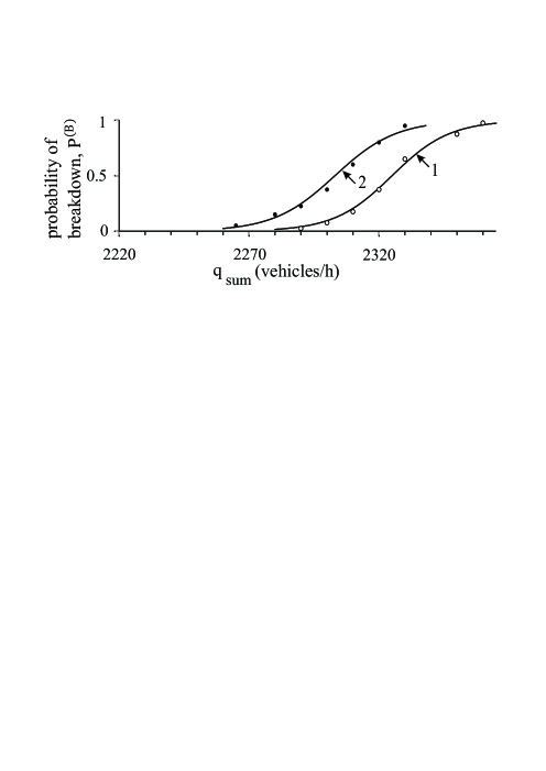
Figure 8: Effect of a single autonomous driving vehicle on the probability $P^{\rm(B)}(q_{\rm sum})$ of traffic breakdown at on-ramp bottleneck on single-lane road in mixed traffic flow. Flow-rate functions of breakdown probability $P^{\rm(B)}(q_{\rm sum})$ (curves 1 and2) are calculated through the change in the on-ramp inflow rate $q_{\rm on}$ at a given flow rate $q_{\rm in}=$ 2000 vehicles/h. Curve 1 is related to traffic flow without autonomous driving vehicles as well as to mixed traffic flow with 2$\%$ of TPACC-vehicles. Curve 2 is related to mixed traffic flow with 2$\%$ of ACC-vehicles with $\tau^{\rm(ACC)}_{\rm d}=$1.3 s. Simulation parameters of ACC and TPACC are identical ones: $\tau^{\rm(ACC)}_{\rm d}=\tau_{\rm p}=$1.3 s, $\tau_{\rm G}=$1.4 s, $K_{1}=0.3\ s^{-2}$ and $K_{2}=K_{\rm\Delta v}=0.6\ s^{-1}$; maximum speed in free flow $v_{\rm free}=30$m/s (108 km/h), vehicle length $d=$7.5 m (see Appendix A); maximum acceleration (deceleration) of ACC- and TPACC-vehicle (under condition that vehicle speed is smaller than some safe speed) $a_{\rm max}=b_{\rm max}=3\ {\rm m}/{\rm s}^{2}$ (see Appendix B).

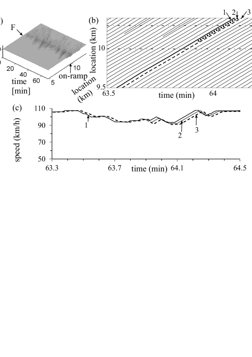
Figure 9: Explanation of the result shown by curve 1 of Fig. 8 that a single TPACC-vehicle does not effect on the probability of traffic breakdown at on-ramp bottleneck in mixed traffic flow. Speed disturbances occurring at on-ramp bottleneck through a single TPACC-vehicle: (a) Speed in space and time. (b) Fragment of vehicle trajectories. (c) Microscopic speeds along vehicle trajectories shown by the same numbers in (b), respectively. In (b, c), vehicles 1 and 2 are human driving vehicles whereas vehicle 3 is TPACC-vehicle. Mixed traffic flow with 2$\%$ of TPACC-vehicles; $q_{\rm in}=$ 2000 vehicles/h, $q_{\rm on}=$ 280 vehicles/h. Other model parameters are the same as those in Fig. 8. In (a, b) the on-ramp merging region that is within road locations $x_{\rm on}\leq x\leq x_{\rm on}^{\rm(e)}$ (see Appendix E) is labeled by $``$on-ramp”.

For calculation of the probability $P^{\rm(B)}(q_{\rm sum})$ of traffic breakdown in free flow at the bottleneck, at each given value of the flow rate downstream of the bottleneck $q_{\rm sum}=q_{\rm in}+q_{\rm on}$ different simulation realizations (runs) $N_{\rm r}=$ 40 during the same time interval for the observing of traffic flow $T_{\rm ob}=$ 30 min have been made (Fig. 8). The different realizations have been performed at the same set of model parameters, however, at different values of the initial values of random function $rand()$ in the traffic flow model (see Appendix A.3 and Appendix A.4). Then, $P^{\rm(B)}(q_{\rm sum})=n_{\rm r}/N_{\rm r}$, where $n_{\rm r}$ is the number of realizations in which traffic breakdown has occurred during the time interval $T_{\rm ob}$ (more detailed explanations of the calculation of the flow-rate function $P^{\rm(B)}(q_{\rm sum})$ have been given in the book [55]).

5.2 Speed Disturbances caused by Single TPACC and Single Classical ACC at Bottleneck

Single TPACC-vehicles moving in such mixed traffic flow cause very small speed disturbances at the bottleneck (Fig. 10 (a–c)). Indeed, we have found that probability of traffic breakdown remains in this mixed flow the same as that in traffic flow consisting of human drivers only (curve 1 in Fig. 8). Thus, single TPACC-vehicles do not effect on the probability of traffic breakdown at the bottleneck.

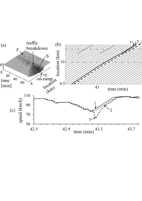
Figure 10: Explanation of the effect of a single classical ACC-vehicle on the probability of traffic breakdown at on-ramp bottleneck in mixed traffic flow associated with curve 2 of Fig. 8. Speed disturbances occurring at on-ramp bottleneck through a single ACC-vehicle (a–c): (a) Speed in space and time. (b) Fragment of vehicle trajectories. (c) Microscopic speeds along vehicle trajectories shown by the same numbers in (b), respectively. In (b, c), vehicles 1 and 2 are human driving vehicles whereas vehicle 3 is ACC-vehicle. Mixed traffic flow with 2$\%$ of ACC-vehicles; $q_{\rm in}=$ 2000 vehicles/h, $q_{\rm on}=$ 280 vehicles/h. Other model parameters for ACC-vehicles are the same as those in Fig. 8. In (a), F – free flow, S – synchronized flow. In (a, b) the on-ramp merging region that is within road locations $x_{\rm on}\leq x\leq x_{\rm on}^{\rm(e)}$ (see Appendix E) is labeled by $``$on-ramp”.

Contrarily to TPACC-vehicles, single classical ACC-vehicles effect considerably on the probability of traffic breakdown at the bottleneck: The probability of traffic breakdown can increase even when $\gamma=2\%$ of classical ACC-vehicles is in mixed traffic flow (curves 2 and 3 in Fig. 8). This is because already a single ACC-vehicle can initiate traffic breakdown at the bottleneck (Fig. 10 (a, b)). This deterioration of traffic flow through classical autonomous driving is explained by the occurrence of a large amplitude speed disturbance caused by a classical ACC-vehicle at the bottleneck (dashed vehicle trajectory 3 in Fig. 10 (b, c)).

5.3 Explanation of Effect of Single Autonomous Driving Vehicle on Speed Disturbance at Bottleneck

The occurrence of very different amplitudes of local speed disturbances caused by the propagation of single classical ACC and TPACC-vehicles through the bottleneck (compare dashed vehicle trajectories 3 in Fig. 9 (b, c) and Fig. 10 (b, c)) can be understood if we consider time functions of the space gap $g(t)$ and the acceleration (deceleration) of the ACC- and TPACC-vehicles (Fig. 11). We can see that after the space gap $g(t)$ due to merging of vehicle 2 decreases abruptly (labeled by $``$merging of vehicle 2” in Figs. 11 (a, c)), both ACC-vehicle and TPACC-vehicle decelerate to increase the space gap $g(t)$. However, the deceleration of ACC-vehicle (Fig. 11 (b)) is considerably stronger than that of TPACC-vehicle (Fig. 11 (d)). The strong deceleration of the ACC-vehicle explains the strong speed reduction of the ACC-vehicle shown in trajectory 3 in Fig. 10 (c).

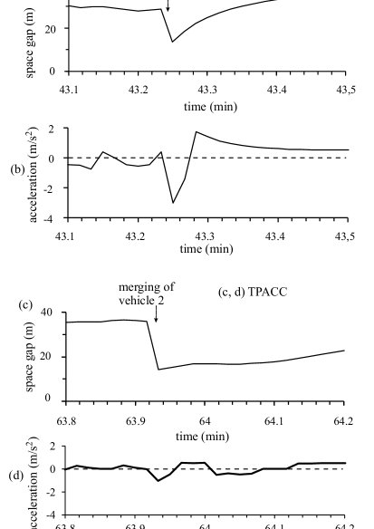
Figure 11: Explanations of speed disturbances caused by propagation of a single autonomous driving vehicle through bottleneck. (a, b) Time functions of the space gap $g(t)$ (a) and the acceleration (deceleration) of the ACC-vehicle (b) related to vehicle trajectory 3 in Fig. 10 (b, c). (c, d) Time functions of the space gap $g(t)$ (c) and the acceleration (deceleration) of the TPACC-vehicle (d) related to vehicle trajectory 3 in Fig. 9 (b, c).

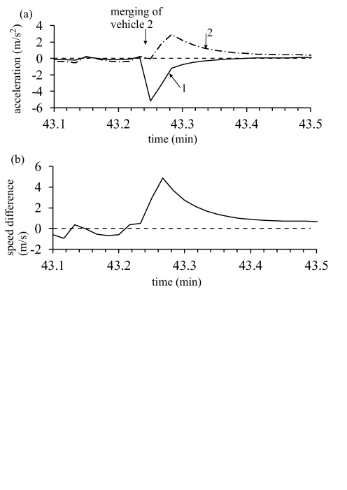
Figure 12: Continuation of Fig. 11 (a, b). (a) Components of formula (4) as time functions; solid curve 1 is time dependence of the term $K_{1}(g-v\tau^{\rm(ACC)}_{\rm d})$, dashed-dotted curve 2 is time dependence of the term $K_{2}(v_{\ell}-v)$. (b) Relative speed between the preceding vehicle and ACC-vehicle. Note that the deceleration calculated through from $K_{1}(g-v\tau^{\rm(ACC)}_{\rm d})$ in (4) reaches a large negative value about $-5.2\ {\rm m/s^{2}}$. It should be noted that as long as condition $v(t)\leq v_{\rm s}(t)$ is satisfied, in the ACC- and TPACC-models there is a limitation of the deceleration by the value $-3\ {\rm m/s^{2}}$. This explains the maximum deceleration of ACC-vehicle $-3\ {\rm m/s^{2}}$ shown in Fig. 11 (b).

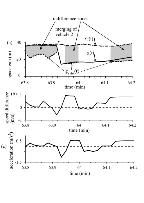
Figure 13: Continuation of Fig. 11 (c, d). (a) Time function of the space gap $g(t)$ of TPACC-vehicle together with indifference zones (gray regions); $G(t)$ is synchronization space gap; $g_{\rm safe}(t)$ (dashed curves) is safe space gap; gray regions show time intervals in which condition (12) for indifference zone is satisfied. (b) Relative speed $\Delta v=v_{\ell}-v$ between the speed of the preceding vehicle and the speed of TPACC-vehicle. (c) Acceleration (deceleration) of TPACC-vehicle given in a larger scale as that in Fig. 11 (d).

To understand this very different microscopic dynamic behavior of ACC- and TPACC-vehicles, we should mention that in the models of ACC- and TPACC-vehicles (see Appendixes B and C) there is a safe speed $v_{\rm s}$ that depends on the speed of the preceding vehicle $v_{\ell}$ and on the space gap $g(t)$ between vehicles: When the vehicle speed of an autonomous driving vehicle satisfies condition $v(t)\leq v_{\rm s}(t)$, then the acceleration (deceleration) of autonomous driving vehicles is determined by formula (4) for ACC and formulas (9) for TPACC. It should be noted that condition $v(t)\leq v_{\rm s}(t)$ is equivalent to condition $g(t)\geq g_{\rm safe}(t)$ for the space gap. For this reason, when the space gap $g(t)<g_{\rm safe}(t)$, then the deceleration of an autonomous driving vehicle should be at least as strong as it follows from the formulation for the safe speed (see Appendix A). The formulation for the safe speed is the same for human driving vehicles, ACC-vehicles, and TPACC-vehicles. The formulation for the safe speed $v_{\rm s}(v_{\ell},g)$ guaranties a collision-less motion of autonomous driving vehicles.

It turns out that although the space gap $g(t)$ due to merging of vehicle 2 decreases abruptly (labeled by $``$merging of vehicle 2” in Fig. 11 (a)), the deceleration of ACC-vehicle determined by formula (4) leads to a stronger vehicle deceleration (Fig. 12 (a)) than it follows from the formulation for the safe speed $v_{\rm s}(v_{\ell},g)$. Therefore, the stronger vehicle deceleration determined by formula (4) is applied. Due to the merging of vehicle 2 from the on-ramp, there two effects that follow each other: (i) the abrupt decrease in the space gap $g(t)$ and (ii) the subsequent increase in the speed difference $\Delta v=v_{\ell}-v$. Because the effect (i) occurs earlier, firstly the deceleration of ACC-vehicle is determined by the term $K_{1}(g-v\tau^{\rm(ACC)}_{\rm d})$ in (4) (curve 1 in Fig. 12 (a)). The subsequent increase in the speed difference $\Delta v=v_{\ell}-v$ that is responsible for the positive value of the term $K_{2}(v_{\ell}-v)$ in (4) (curve 2 in Fig. 12 (a)) cannot prevent the strong deceleration of ACC-vehicle mentioned above (Fig. 11 (b)).

Microscopic behavior of TPACC-vehicle (Fig. 13) is qualitatively different from that of ACC-vehicle (Fig. 12) discussed above. Before vehicle 2 merges onto the main road, the space gap $g(t)$ of TPACC-vehicle has satisfied condition (12) of the indifference zone (first gray region in Fig. 13 (a) that is related to time interval before labeling $``$merging of vehicle 2”). After the space gap $g(t)$ due to merging of vehicle 2 decreases abruptly (labeled by $``$merging of vehicle 2” in Fig. 13 (a)), condition $g(t)<g_{\rm safe}(t)$ is satisfied for TPACC-vehicle. In contrast with ACC-vehicle, the deceleration of TPACC-vehicle determined by formula (9) leads to a weaker vehicle deceleration than it follows from the formulation for the safe speed $v_{\rm s}(v_{\ell},g)$. As a result, TPACC-vehicle decelerates in accordance with the formulation of the safe speed $v_{\rm s}(v_{\ell},g)$.

As mentioned, the formulation of the safe speed $v_{\rm s}(v_{\ell},g)$ is related to the behavior of a human driving vehicle (Appendix A.6). The safe speed $v_{\rm s}(v_{\ell},g)$ depends considerably stronger on the speed difference $\Delta v=v_{\ell}-v$ than on the space gap $g(t)$. When under condition $g(t)<g_{\rm safe}(t)$ the speed difference $\Delta v=v_{\ell}-v\geq 0$, the deceleration of the TPACC-vehicle associated with the safety conditions (Figs. 11 (d) and 13 (c)) is considerably smaller than the deceleration of the ACC-vehicle given by formula (4) (Figs. 11 (b) and 12 (a)). Moreover, when the value $\Delta v>0$ is large enough, condition $g(t)>g_{\rm safe}(t)$ for the indifference zone is satisfied (second gray region in Fig. 13 (a)). The time evolution of the speed difference $\Delta v(t)$ (Fig. 13 (b)) determines in the large degree the deceleration (acceleration) of TPACC-vehicle (Fig. 13 (c)). Over time, there is an alternation of indifference zones (12) (in which formulas (9) are valid) and safety deceleration regions (in which the TPACC-vehicle moves in accordance with the formulation for the safe speed) (Fig. 13 (a)). This alternation determines a slowly increase in the space gap $g(t)$ of TPACC-vehicle (Fig. 13 (a)). Finally, TPACC-vehicle moves in the indifference zone only.

Both safety conditions of TPACC-vehicle and car-following behavior (9) at the bottleneck (trajectory 3 in Fig. 9 (c)) are similar as those for human driving vehicles (trajectories 1 and 2 in Fig. 9 (c)).

• For this reason, we can consider autonomous driving in the framework of the three-phase theory (TPACC) as $``$autonomous driving learning from real driving behavior”.

In particular, when due to the vehicle merging the space gap $g(t)$ becomes shorter than the safe space gap $g_{\rm safe}$ and the speed difference $\Delta v=v_{\ell}-v\approx 0$, a TPACC vehicle decelerates as slowly as a human driving vehicle does. This explains why in simulations of mixed traffic flow with TPACC vehicles presented in Fig. 9 (b, c) no large speed disturbances occur at the bottleneck. This explains also why in contrast with classical autonomous driving (curve 2 in Fig. 8) single TPACC-vehicles do not effect on the probability of traffic breakdown at the bottleneck in mixed traffic flow (curve 1 in Fig. 8).

6 Effect of Dynamic Parameters of Classical ACC and TPACC on Traffic Breakdown at Bottleneck

6.1 Time Headway of ACC and Breakdown Probability

In Sec. 5 we have shown that traffic breakdown can be caused by a single classical ACC-vehicle at the on-ramp bottleneck with the breakdown probability $P^{\rm(B)}>0$, whereas the probability of traffic breakdown through TPACC-vehicles at the same parameters is equal to zero. However, this result is related to a chosen value of a desired time headway $\tau^{\rm(ACC)}_{\rm d}=$ 1.3 s in Eq. 4 (curve 2 in Figs. 8 and 14).

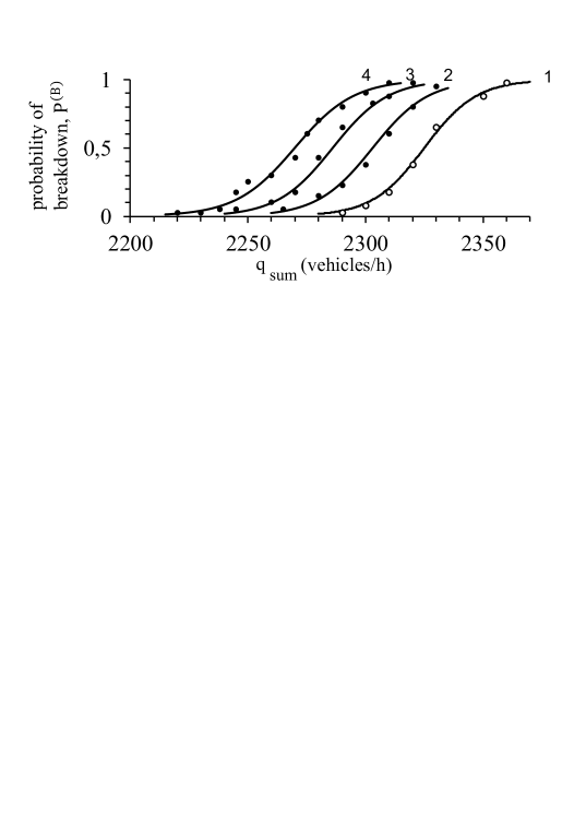
Figure 14: Dependence of the probability $P^{\rm(B)}(q_{\rm sum})$ of traffic breakdown at on-ramp bottleneck on single-lane road on ACC and TPACC parameters. Flow-rate functions of breakdown probability $P^{\rm(B)}(q_{\rm sum})$ (curves 1–4) are calculated through the change in the on-ramp inflow rate $q_{\rm on}$ at a given flow rate $q_{\rm in}=$ 2000 vehicles/h. Curve 1 is related to traffic flow without autonomous driving vehicles as well as to mixed traffic flow with 2$\%$ of TPACC-vehicles. Curves 2–4 are related to mixed traffic flow with 2$\%$ of ACC-vehicles. Simulation parameters of ACC are: curve 2 is the same as curve 2 in Fig 8; curve 3 is related to $\tau^{\rm(ACC)}_{\rm d}=$1.5 s; curve 4 is related to $\tau^{\rm(ACC)}_{\rm d}=$2 s. For curve 1 with 2$\%$ of TPACC-vehicles in the mixed traffic flow the following sets of TPACC-parameters ($\tau_{\rm p},\ \tau_{\rm G}$) have been used: (1.3,  1.4) s, (1.5,  1.6) s, (2,  2.2) s. Other model parameters are the same as those in Fig 8.

Therefore, a question arises whether this result remains for a broad range of the desired time headway of ACC and the related range of time headway of TPACC. A study of this question for a range of the desired time headway of ACC

$$1.3\ \leq\tau^{\rm(ACC)}_{\rm d}\leq\ {\rm 2\ s}$$ (14)

shows that at any desired time headway of ACC (14) the probability of traffic breakdown caused by single ACC-vehicles is larger than in traffic flow of human drivers. Moreover, the longer the desired time headway of ACC $\tau^{\rm(ACC)}_{\rm d}$ is, the larger the probability of traffic breakdown at the same other model parameters (curves 2–4 in Fig. 14).

Contrarily to classical ACC-vehicles, when, in accordance with (14), we choose parameters of TPACC-model (9) in the ranges

$$1.3\ \leq\tau_{\rm p}\leq\ {\rm 2\ s},$$ (15)

$$1.4\ \leq\tau_{\rm G}\leq\ {\rm 2.2\ s},$$ (16)

then no noticeable change in the probability of traffic breakdown through TPACC-vehicles can be found (curve 1 in Fig. 14).

6.2 Analysis of Disturbances caused by Classical ACC at Bottleneck

To understand the dependence of the ACC parameters on traffic breakdown (curves 2–4 in Fig. 14), we have chosen the on-ramp inflow rate $q_{\rm on}=$ 280 vehicles/h and the flow rate on the main road $q_{\rm in}=$ 2000 vehicles/h at which the probability of traffic breakdown $P^{\rm(B)}$ at the bottleneck is equal to zero for mixed traffic flow with $2\%$ TPACC-vehicles (curve 1 in Fig. 14), whereas the probability of traffic breakdown in mixed traffic flow with $2\%$ ACC-vehicles satisfies conditions

$$0<P^{\rm(B)}<1$$ (17)

for any chosen desired time headway of ACC in (14) (curves 2–4 in Fig. 14).

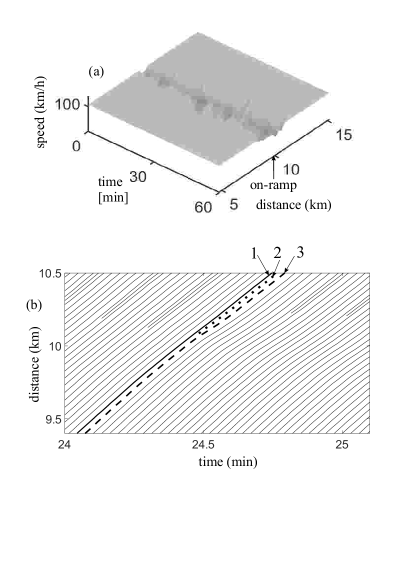
Figure 15: One of the realizations of simulation of mixed traffic flow in which under conditions (17) no traffic breakdown is observed during the observation time interval $T_{\rm ob}=$ 60 min in mixed traffic flow with $2\%$ ACC-vehicles with $\tau^{\rm(ACC)}_{\rm d}$1.3 s: (a) Vehicle speed in space and time. (b) Fragment of vehicle trajectories. The on-ramp inflow rate $q_{\rm on}=$ 280 vehicles/h and the flow rate on the main road $q_{\rm in}=$ 2000 vehicles/h. Other model parameters are the same as those in Fig. 14.

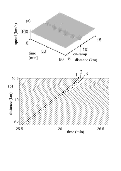
Figure 16: One of the realizations of simulation of mixed traffic flow in which under conditions (17) no traffic breakdown is observed during the observation time interval $T_{\rm ob}=$ 60 min in mixed traffic flow with $2\%$ ACC-vehicles with $\tau^{\rm(ACC)}_{\rm d}=$1.5 s: (a) Vehicle speed in space and time. (b) Fragment of vehicle trajectories. The on-ramp inflow rate $q_{\rm on}=$ 280 vehicles/h and the flow rate on the main road $q_{\rm in}=$ 2000 vehicles/h. Other model parameters are the same as those in Fig. 14.

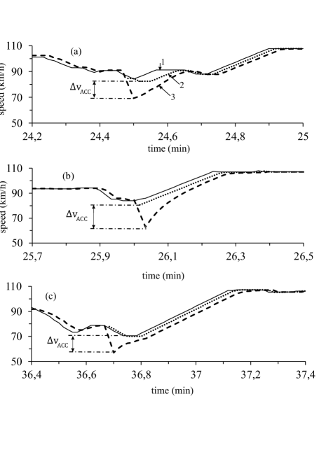
Figure 17: Microscopic speed of ACC-vehicles following a human driving vehicle that merges from the on-ramp on the main road for different values $\tau^{\rm(ACC)}_{\rm d}$: (a) The simulation realization shown in Fig. 15 for $\tau^{\rm(ACC)}_{\rm d}=$1.3 s. (b) The simulation realization shown in Fig. 16 for $\tau^{\rm(ACC)}_{\rm d}=$1.5 s. (c) One of the simulation realization for $\tau^{\rm(ACC)}_{\rm d}=$2 s. The on-ramp inflow rate $q_{\rm on}=$ 280 vehicles/h and the flow rate on the main road $q_{\rm in}=$ 2000 vehicles/h. Other model parameters are the same as those in Fig. 14.

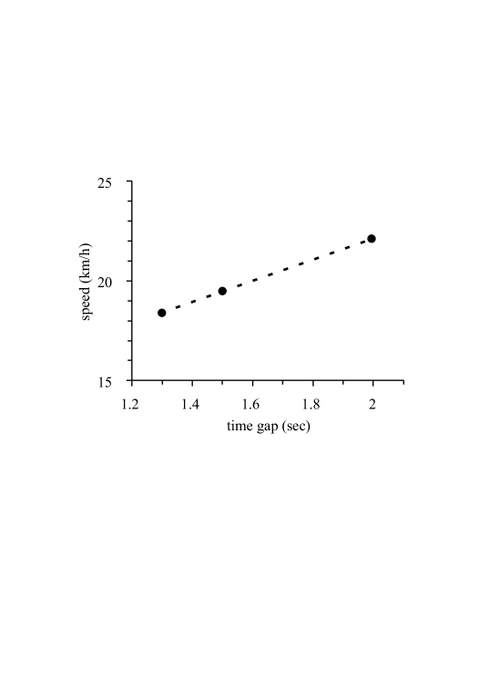
Figure 18: Mean values of the amplitude of local speed reduction of ACC-vehicles following a human driving vehicle that merges from the on-ramp on the main road for different values $\tau^{\rm(ACC)}_{\rm d}$ (black circles) that are the same as those in Fig. 17.

Conditions (17) allows us to choose those simulation realizations for mixed traffic flow with $2\%$ ACC-vehicles in which no traffic breakdown is observed during the observation time interval $T_{\rm ob}$ for any chosen desired time headway of ACC within the range (14). For these simulation realizations, we make a statistical analysis of the amplitudes of speed disturbances caused by ACC-vehicles for the case, when an ACC-vehicle follows a human driving vehicle that merges from the on-ramp onto the main road. Examples of a simulation realization for $\tau^{\rm(ACC)}_{\rm d}=$1.3 s and a simulation realization for $\tau^{\rm(ACC)}_{\rm d}=$1.5 s are shown, respectively, in Figs. 15 and 16.

As the amplitude (denoted by $\Delta v_{\rm ACC}$) of a speed disturbance caused by an ACC-vehicle, we consider a difference between the speed of vehicle 2 that merges from the on-ramp onto the main road and the minimum speed of the ACC-vehicle (vehicle 3 in Fig. 17) following this merging vehicle 2:

$$\Delta v_{\rm ACC}=v_{\ell,m}-v^{\rm(ACC)}_{\rm min},$$ (18)

where $v_{\ell,m}$ is the speed of vehicle 2 at time step $n=m$ when vehicle 2 becomes the preceding vehicle for the ACC-vehicle, $v^{\rm(ACC)}_{\rm min}$ is the minimum speed of the ACC-vehicle.

As in Fig. 10, in Fig. 15 (b) vehicles 1 and 2 are human driving vehicles, whereas vehicle 3 is ACC-vehicle. The microscopic ACC-vehicle speed (vehicle 3 in Fig. 15 (b)) as a time-function exhibits a relatively large amplitude of a local speed reduction (Fig. 17 (a)). A large amplitude of a local speed reduction exhibits also an ACC-vehicle with $\tau^{\rm(ACC)}_{\rm d}=$1.5 s as it is shown in Fig. 17 (b).

Qualitative the same simulation results as that in Fig. 15 have been found for simulation realizations in which no traffic breakdown is observed during the observation time interval $T_{\rm ob}=$ 60 min in mixed traffic flow with $2\%$ ACC-vehicles satisfying conditions (17) for any chosen desired time headway of ACC within the range (14): When a human driving vehicle merges from the on-ramp onto the main road, then an ACC-vehicle that follows this vehicle exhibits always a large amplitude of a local speed reduction. An example for a large amplitude of a local speed reduction that shows an ACC-vehicle with $\tau^{\rm(ACC)}_{\rm d}=$ 2 s is shown in Fig. 17 (c).

The amplitude of a local speed reduction that shows an ACC-vehicle following a human driving vehicle that merges from the on-ramp onto the main road is a random value that depends on a simulation realization. Random amplitudes of the local speed disturbances are realized for each of the chosen desired time headway of ACC $\tau^{\rm(ACC)}_{\rm d}$. This means that each of the amplitudes of local speed disturbances of the ACC-vehicles shown in Fig. 17 are related to the associated simulation realization only.

For this reason, we have made a statistical analysis of the amplitude of the local speed disturbances: For each of the chosen desired time headway of ACC $\tau^{\rm(ACC)}_{\rm d}$ shown in Fig. 17, we have studied $N_{\rm r}=$ 40 different random simulation realizations. The mean values of the amplitude of local speed disturbance found from these random realizations are presented by black circles in Fig. 18.

We can see from dash line in Fig. 18 that the longer the chosen desired time headway of ACC $\tau^{\rm(ACC)}_{\rm d}$ is, the larger the mean amplitude of the local speed disturbance caused by the ACC-vehicle at the on-ramp bottleneck. On the other hand, the larger the mean amplitude of the local speed disturbance (local speed reduction) at the bottleneck is, the larger the probability of traffic breakdown in the metastable free flow at the bottleneck. This result explains the increase in the probability of traffic breakdown at the bottleneck with the increase in the value of the desired time headway of ACC $\tau^{\rm(ACC)}_{\rm d}$ shown in Fig. 14.

7 Effect of Dynamic Rules of Autonomous Driving on Disturbances at Bottleneck

We have shown that the longer the chosen desired time headway of ACC $\tau^{\rm(ACC)}_{\rm d}$ is, the larger the mean amplitude of the local speed disturbance caused by the ACC-vehicle at the on-ramp bottleneck (Fig. 18).

Contrarily to this feature of the classical ACC, we have found that the mean amplitude of the local speed disturbance caused by the TPACC-vehicle at the on-ramp bottleneck does not almost depend on the parameters of TPACC within the parameter ranges (15), (16). For this reason, some effect of single TPACC-vehicles on the probability of traffic breakdown at the on-ramp bottleneck cannot be found (curve 1 in Fig. 14).

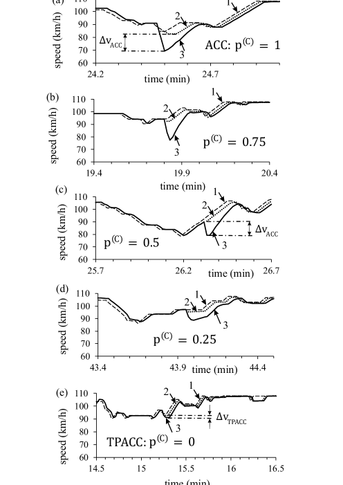
Figure 19: Local speed reduction caused by ACC-vehicle at on-ramp bottleneck related to ACC-model (21)–(25) in one of simulation realizations for five different values $p^{\rm(C)}=$ 0 (a), 0.25 (b), 0.5 (c), 0.75 (d), and 1 (e). Vehicles 1 and 2 are human driving vehicles, vehicle 3 is the ACC-vehicle. Model parameters are: $\tau_{\rm G}=$1.4 s, $\tau_{\rm p}=$1.3 s, $K_{1}=$0.3 $s^{-2}$, $K_{2}=K_{\rm\Delta v}=$0.6$s^{-1}$. Other model parameters are the same as those in Fig. 14.

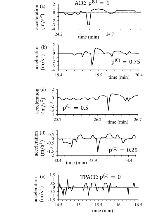
Figure 20: Deceleration (acceleration) of ACC-vehicle in the same simulation realizations as those in Fig. 19, respectively, for five different values $p^{\rm(C)}=$ 0 (a), 0.25 (b), 0.5 (c), 0.75 (d), and 1 (e).

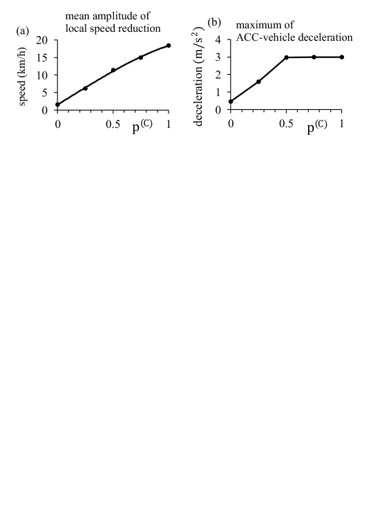
Figure 21: Characteristics of local speed reductions caused by ACC-vehicles at on-ramp bottleneck as a function of value $p^{\rm(C)}$ for model parameters of Fig. 19: (a) Mean amplitude of local speed reduction. (b) Mean value of maximum ACC-vehicle deceleration within local speed reduction.

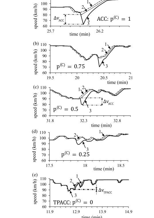
Figure 22: Local speed reduction caused by ACC-vehicle at on-ramp bottleneck related to ACC-model (21)–(25) in one of simulation realizations for five different values $p^{\rm(C)}=$ 0 (a), 0.25 (b), 0.5 (c), 0.75 (d), and 1 (e). Vehicles 1 and 2 are human driving vehicles, vehicle 3 is the ACC-vehicle. $\tau_{\rm G}=$1.6 s, $\tau_{\rm p}=$1.5 s. Other model parameters are the same as those in Fig. 19.

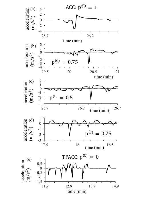
Figure 23: Deceleration (acceleration) of ACC-vehicle in the same simulation realizations as those in Fig. 22, respectively, for five different values $p^{\rm(C)}=$ 0 (a), 0.25 (b), 0.5 (c), 0.75 (d), and 1 (e).

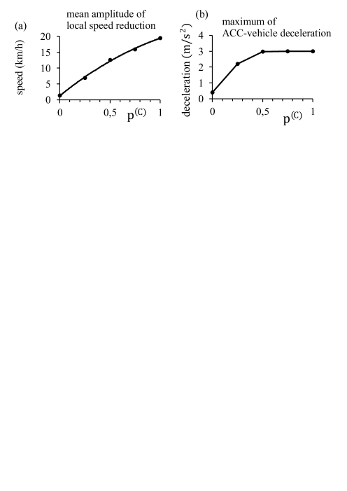
Figure 24: Characteristics of local speed reductions caused by ACC-vehicles at on-ramp bottleneck as a function of value $p^{\rm(C)}$ for model parameters of Fig. 22: (a) Mean amplitude of local speed reduction. (b) Mean value of maximum ACC-vehicle deceleration within local speed reduction.

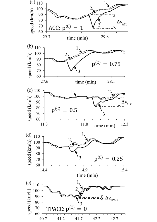
Figure 25: Local speed reduction caused by ACC-vehicle at on-ramp bottleneck related to ACC-model (21)–(25) in one of simulation realizations for five different values $p^{\rm(C)}=$ 0 (a), 0.25 (b), 0.5 (c), 0.75 (d), and 1 (e). Vehicles 1 and 2 are human driving vehicles, vehicle 3 is the ACC-vehicle. $\tau_{\rm G}=$2.2 s, $\tau_{\rm p}=$2 s. Other model parameters are the same as those in Fig. 19.

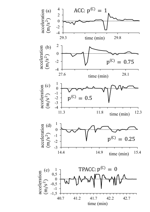
Figure 26: Deceleration (acceleration) of ACC-vehicle in the same simulation realizations as those in Fig. 25, respectively, for five different values $p^{\rm(C)}=$ 0 (a), 0.25 (b), 0.5 (c), 0.75 (d), and 1 (e).

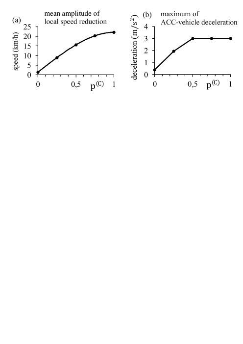
Figure 27: Characteristics of local speed reductions caused by ACC-vehicles at on-ramp bottleneck as a function of value $p^{\rm(C)}$ for model parameters of Fig. 25: (a) Mean amplitude of local speed reduction. (b) Mean value of maximum ACC-vehicle deceleration within local speed reduction.

The mathematical difference between dynamic rules of classical ACC (4) and TPACC (9) seems to be small. Therefore, the following question arises: How can such seeming small mathematical difference between dynamic rules of classical ACC and TPACC lead to such a large effect on the local speed disturbances in free flow and, respectively, to a large effect on the probability of traffic breakdown at the bottleneck?

To answer this question, we introduce a model of ACC, in which rather than a classical formula (4) for ACC-acceleration, the ACC-acceleration denoted by $a^{\rm(C)}$ is given by the following formula:

$$a^{\rm(C)}=\left\{\begin{array}[]{ll}\tilde{a}^{\rm(C)}&\textrm{at $g\leq G^{\rm(C)}$,}\\ a^{\rm(ACC)}&\textrm{at $g>G^{\rm(C)}$},\\ \end{array}\right.$$ (21)

where

$$\tilde{a}^{\rm(C)}=a^{\rm(2D)}(1-p^{\rm(C)})+a^{\rm(ACC)}p^{\rm(C)},$$ (22)

$$a^{\rm(2D)}=K_{\rm\Delta v}\Delta v,$$ (23)

$$a^{\rm(ACC)}=K_{1}(g-v\tau_{\rm p})+K_{2}\Delta v,$$ (24)

$$G^{\rm(C)}=G(1-p^{\rm(C)})+v\tau_{\rm p}p^{\rm(C)},$$ (25)

a constant parameter $p^{\rm(C)}$ satisfies condition

$$0\leq p^{\rm(C)}\leq 1,$$ (26)

it is also assumed that conditions (10) and (11) are satisfied. A discrete in time version of the model of ACC (21)–(25) used in simulations is presented in Appendix D.

It should be emphasized that at $p^{\rm(C)}=1$ and $\tau^{\rm(ACC)}_{\rm d}=\tau_{\rm p}$ the ACC-model (21)–(25) transforms to the classical model for ACC (4). Contrarily, at $p^{\rm(C)}=0$ the ACC-model (21)–(25) transforms to the TPACC-model (9). In other words, in the ACC model (21)–(25) by the increasing in parameter $p^{\rm(C)}$ (26) the rules for ACC-vehicle motion (21)–(25) are continuously changed from the rules for the TPACC-model (9) at $p^{\rm(C)}=0$ to the rules for the classical ACC-model (4) at $p^{\rm(C)}=1$.

We have found that the larger the value $p^{\rm(C)}$ in the ACC-model (21)–(25) is, the stronger on average the reaction of the ACC-vehicle (vehicle 3 in Figs. 19,  22, and 25) on the difference between the desired time headway of ACC $\tau^{\rm(ACC)}_{\rm d}=\tau_{\rm p}$ and a current time headway to the preceding vehicle (vehicle 2) is. This result remains for different values $\tau_{\rm p}$ related to time headway ranges (14), (15) and (16), respectively (Figs. 19–27). In particular, we have found the following general results:

(i) When the parameter $p^{\rm(C)}$ increases from $p^{\rm(C)}=0$ (TPACC) to $p^{\rm(C)}=1$ (classical ACC), the amplitude of a local speed reduction (Figs. 19,  22, and 25) caused by the ACC-vehicle (21)–(25) at the on-ramp bottleneck increases continuously. Therefore, the increase in the mean amplitude of a local speed reduction caused by the ACC-vehicle (21)–(25) at the on-ramp bottleneck is almost linear function of the increase in parameter $p^{\rm(C)}$ (Figs. 21 (a),  24 (a), and 27 (a)).

(ii) When the parameter $p^{\rm(C)}$ increases from $p^{\rm(C)}=0$ (TPACC) to $p^{\rm(C)}=1$ (classical ACC), the deceleration of the ACC-vehicle (21)–(25) within a local speed reduction caused by the ACC-vehicle (21)–(25) at the bottleneck increases strongly. For values of $p^{\rm(C)}$ that are close to 1, the deceleration of the ACC-vehicle reaches the maximum value $-3\ \rm ms^{-2}$ (Figs. 21 (b),  24 (b), and 27 (b)) chosen in the model of the ACC-vehicle (21)–(25) for usual driving conditions. When for $p^{\rm(C)}=1$ (classical ACC) the desired time headway of ACC $\tau^{\rm(ACC)}_{\rm d}=\tau_{\rm p}$ increases from 1.3 s to 2 s, the duration of the time interval within which the deceleration of the ACC-vehicle reaches the maximum value $-3\ \rm ms^{-2}$ increases considerably (Figs. 20 (b),  23 (b), and 26 (b)).

This comparison of classical ACC (4) with TPACC (9) confirms that the stronger the reaction of ACC-vehicle on the difference between the desired time headway of ACC $\tau^{\rm(ACC)}_{\rm d}$ and a current time headway to the preceding vehicle, the larger on average the amplitude of local speed reduction caused by the ACC-vehicle at the bottleneck and, therefore, the larger the probability of traffic breakdown at the bottleneck. Indeed, within the time headway range (13) TPACC-vehicle ($p^{\rm(C)}=0$) does no react on a current time headway to the preceding vehicle. Due to the existence of such an indifferent zone in car-following the TPACC-vehicle either does not produce a local speed reduction at the bottleneck at all or the local speed reduction caused by the TPACC-vehicle is of a very small amplitude.

Contrarily to TPACC ($p^{\rm(C)}=0$), when $p^{\rm(C)}>0$ and it increases continuously, the deceleration of the ACC-vehicle (21)–(25) at the bottleneck caused by the difference between the desired time headway of ACC-vehicle $\tau^{\rm(ACC)}_{\rm d}=\tau_{\rm p}$ and a current time headway to the preceding vehicle increases on average continuously (Figs. 20 (a–d),  23 (a–d), and 26 (a–d)). This leads to the largest mean amplitude of a local speed reduction caused by the ACC-vehicle (21)–(25) at the bottleneck at $p^{\rm(C)}=1$ (Figs. 21 (a),  24 (a), and 27 (a)). This explains the following results found in simulations: For a given time headway $\tau^{\rm(ACC)}_{\rm d}$, the larger the value $p^{\rm(C)}$ in the model of the ACC-vehicle (21)–(25), the larger the probability of traffic breakdown at the bottleneck for the same other model parameters. This increase in the probability of traffic breakdown becomes the stronger, the longer time headway $\tau^{\rm(ACC)}_{\rm d}=\tau_{\rm p}$ is in the ACC-model (21)–(25). This result correlates with the conclusion of Sec. 6.1 that the longer the desired time headway $\tau^{\rm(ACC)}_{\rm d}$ of classical ACC ($p^{\rm(C)}=1$ in (21)–(25)), the stronger the increase in the probability of traffic breakdown caused by a single classical ACC-vehicle at the bottleneck (curves 2–4 in Fig. 14).

8 Platoons of Autonomous Driving Vehicles and Probability of Traffic Breakdown in Mixed Traffic Flow

If the share of autonomous driving vehicles in mixed traffic flow increases, (Fig. 28), the probability of traffic breakdown caused by ACC-vehicles that deteriorate traffic can increase considerably (curve 3 in Fig. 28).

Contrarily to classical ACC-vehicles, long enough platoons of TPACC-vehicles in mixed traffic flow decrease the breakdown probability (curve 2 in Fig. 28). This is explained by small local speed disturbances caused by TPACC-vehicles in mixed free flow at the bottleneck in comparison with large local speed disturbances caused by classical ACC-vehicles, as already discussed in Sec. 7.

In particular, the reduction of the probability of traffic breakdown in mixed traffic flow at the bottleneck though already small platoons of TPACC-vehicles (curve 2 in Fig. 28) is explained by the speed adaptation effect of the three-phase theory that is the basis of TPACC (9): At each vehicle speed, the TPACC-vehicle makes an arbitrary choice in time headway that satisfies conditions (13). In other words, the TPACC-vehicle accepts different values of time headway at different times and does not control a fixed time headway to the preceding vehicle. This dynamic behavior of a platoon of TPACC-vehicles decreases the amplitude of local speed disturbances at the bottleneck [73]. This explains why, in contrast to classical ACC-vehicles, TPACC-vehicles decrease the probability of traffic breakdown in mixed traffic flow.

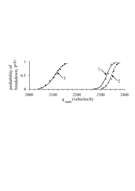
Figure 28: Probability of traffic breakdown at on-ramp bottleneck as a function of the flow rate $q_{\rm sum}=q_{\rm in}+q_{\rm on}$ at a given on-ramp inflow rate $q_{\rm on}=$ 320 vehicles/h in mixed traffic flow with 20$\%$ autonomous driving vehicles: Curve 1 is related to traffic flow without autonomous driving vehicles. Curves 2 and 3 are related to mixed traffic flow with TPACC-vehicles (curve 2) and ACC-vehicles (curve 3). Simulation parameters of ACC and TPACC are, respectively, the same as those in Fig. 8.

We note that in mixed traffic flow with $\gamma=20\%$ of classical ACC-vehicles at the on-ramp inflow rate $q_{\rm on}=$ 320 vehicles/h the probability of traffic breakdown reaches the maximum value $P^{\rm(B)}=1$ already at $q_{\rm in}=$ 1830 vehicles/h (curve 3 in Fig. 28). However, it should be noted that at parameters of ACC-vehicles used for simulations of curve 3 in Fig. 28 any platoon of the ACC-vehicles satisfies condition (5) for string stability. This means that if, rather than mixed traffic flow (curve 3 in Fig. 28), we consider free flow consisting of $\gamma=100\%$ of classical ACC-vehicles, then in accordance with results of Ref. [73] no traffic breakdown at $q_{\rm on}=$ 320 vehicles/h and $q_{\rm in}=$ 1830 vehicles/h is realized at the bottleneck. The latter result remains true, even when the flow rate upstream of the bottleneck increases to $q_{\rm in}=$ 2000 vehicles/h.

9 Traffic Stream Characteristics of Mixed Traffic Flow

In traffic engineering, the flow–density (the fundamental diagram) and speed–flow relationships are often used to study the effect of traffic control and management on macroscopic traffic stream characteristics [26, 27, 28, 32, 33, 34]. To answer a question of how traffic flow is affected when the TPACC strategy versus the ACC strategy is considered [73, 74], in this section we make a study of traffic stream flow characteristics related to simulations of mixed traffic flow presented in Figs. 8 and 28. For simplicity, we consider below macroscopic traffic stream characteristics with the use of speed–flow relationships. The associated flow–density flow–density relationships (the fundamental diagram) can be found in [73].

9.1 Mixed Traffic Flow with 2$\%$ Autonomous Driving Vehicles

In Fig. 29 (a), we show a part of the speed–flow relationship for larger flow rates in free flow without autonomous driving vehicles. It turns out that traffic stream flow characteristics are identical for traffic without autonomous driving vehicles and for mixed traffic with 2$\%$ of TPACC-vehicles: Single TPACC-vehicles do not affect the stream flow characteristics in free flow (Fig. 29 (a)). This corresponds results of Sec. 5: 2$\%$ of TPACC-vehicles do not affect the probability of traffic breakdown $P^{\rm(B)}(q_{\rm sum})$ (curve 1 shown in Fig. 8).

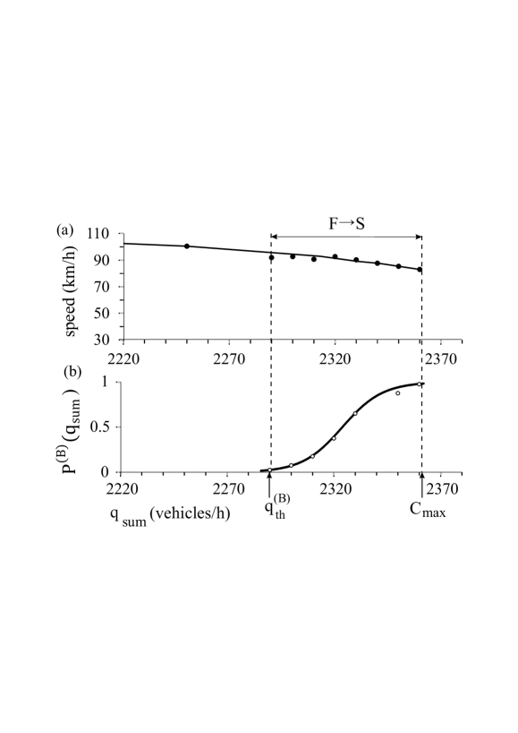
Figure 29: Stream flow characteristics of free flow on single-lane road with on-ramp bottleneck in traffic without autonomous driving vehicles and in mixed traffic with 2$\%$ of TPACC-vehicles: (a) A part of speed–flow relationship for larger flow rates. (b) The breakdown probability $P^{\rm(B)}(q_{\rm sum})$; function $P^{\rm(B)}(q_{\rm sum})$ is curve 1 from Fig. 8. Traffic stream flow characteristics have been calculated as follows. At each given flow rate $q_{\rm sum}$ (black points on the characteristics), 5-min averaged data for the speed, density, and flow rate have been measured with the use of a virtual road detector installed at the end of the on-ramp merging region $x=$ 10.3 km. The data has been measured only during time interval within which free flow has been observed in a simulation realization. Then, as by the calculation of $P^{\rm(B)}(q_{\rm sum})$ in Fig. 8, $N_{\rm r}=$ 40 different realizations have been simulated for each of the chosen flow rates $q_{\rm sum}$. This allows us to make a statistical analysis of the average speed and density in the traffic stream. Black points on the speed–flow relationship are related to the average values of the speed and density derived from this statistical analysis. Other model parameters are the same as those in Fig. 8. Calculated values: $q^{\rm(B)}_{\rm th,\ TPACC}=q^{\rm(B)}_{\rm th}=2290$ and $C_{\rm max,\ TPACC}=C_{\rm max}=2360$ vehicles/h.

In the three-phase theory (see books [53, 54, 55] and [80, 79]), there is a deep connection between the flow-rate dependence of the probability of traffic breakdown $P^{\rm(B)}(q_{\rm sum})$ (Fig. 8) and the overall flow as well as other traffic stream flow characteristics (Fig. 29). In particular, on traffic stream flow characteristics one should distinguish a flow rate range (Figs. 29 and 30)

$$q^{\rm(B)}_{\rm th}\leq q_{\rm sum}\leq C_{\rm max}.$$ (27)

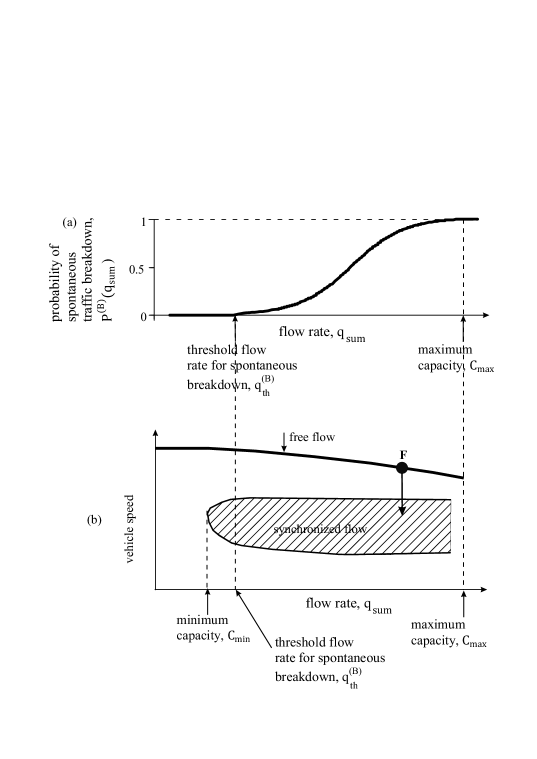
Figure 30: Qualitative explanation of condition (27): (a) Qualitative flow-rate function of the breakdown probability $P^{\rm(B)}(q_{\rm sum})$. (b) Z-Characteristic of traffic breakdown with states for free flow and synchronized flow taken from Fig. 2. Adapted from [55].

Within the flow rate range (1), free flow is in a metastable state with respect to traffic breakdown (F$\rightarrow$S transition) at the bottleneck (Fig. 30). A characteristic flow rate $q_{\rm sum}=q^{\rm(B)}_{\rm th}$ in (27) is a threshold flow rate for spontaneous traffic breakdown at the bottleneck: At $q_{\rm sum}<q^{\rm(B)}_{\rm th}$ the breakdown probability $P^{\rm(B)}=0$ (Fig. 30 (a)), i.e., no spontaneous traffic breakdown can occur during a time interval of the observation of traffic flow $T_{\rm ob}$.

A characteristic flow rate $q_{\rm sum}=C_{\rm max}$ in (1) and (27) is the maximum highway capacity (Figs. 2 and 30): At $q_{\rm sum}\geq C_{\rm max}$ the breakdown probability $P^{\rm(B)}=1$ (Fig. 30 (a)), i.e., spontaneous traffic breakdown does occur at the bottleneck during the time interval $T_{\rm ob}$.

The larger the values $q^{\rm(B)}_{\rm th}$ and $C_{\rm max}$ for the traffic stream, the larger is on average the overall flow. Therefore, the characteristic flow rates $q^{\rm(B)}_{\rm th}$ and $C_{\rm max}$, which determine the boundaries of the flow rate range (27) (Fig. 30), are basic statistical characteristics of the overall flow in the traffic stream in the framework of the three-phase theory.

For the further analysis, we denote the flow rate range (27) on traffic stream characteristics by the arrow $``$F$\rightarrow$S” (Figs. 29, 31, and 32).

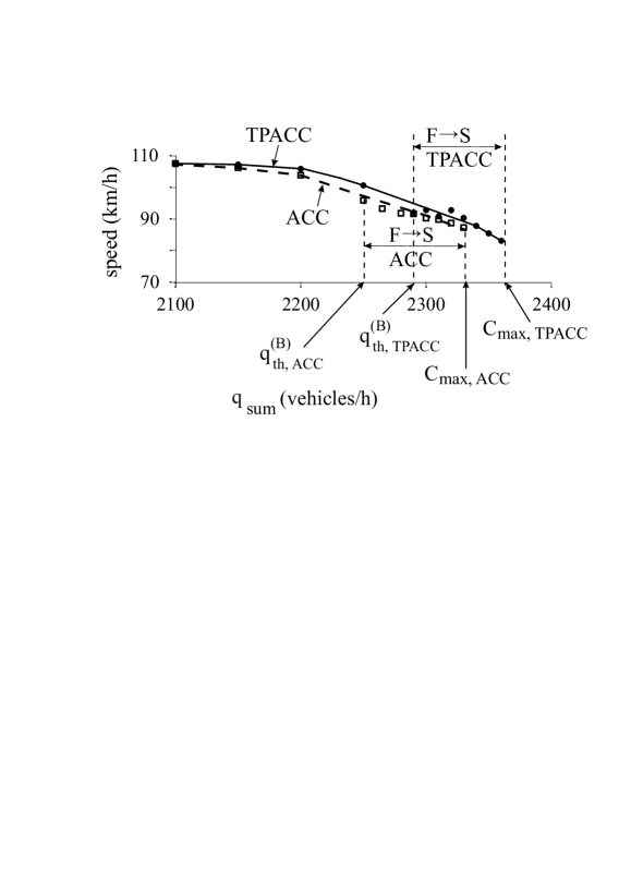
Figure 31: Comparison of traffic stream flow characteristics for free flow on single-lane road with on-ramp bottleneck in mixed traffic with 2$\%$ of autonomous driving vehicles. A parts of speed–flow relationship for larger flow rates. Solid curves $``$TPACC” are related to TPACC-vehicles. Dashed curves $``$ACC” are related to classical ACC-vehicles. Stream flow characteristics have been calculated as explained in caption to Fig. 29. Other model parameters are the same as those in Fig. 8. Calculated values: $q^{\rm(B)}_{\rm th,\ TPACC}=2290$ and $C_{\rm max,\ TPACC}=2360$ vehicles/h; $q^{\rm(B)}_{\rm th,\ ACC}=2265$ and $C_{\rm max,\ ACC}=2330$ vehicles/h.

We denote the statistical characteristics of the overall flow $q^{\rm(B)}_{\rm th}$, $C_{\rm max}$ in (27) for mixed traffic flow by $q^{\rm(B)}_{\rm th,\ TPACC}$, $C_{\rm max,\ TPACC}$, when autonomous driving vehicles are TPACC-vehicles, and by $q^{\rm(B)}_{\rm th,\ ACC}$, $C_{\rm max,\ ACC}$ for classical ACC-vehicles, respectively. We have found that the overall flow characteristics do not change on average in mixed traffic with 2$\%$ of TPACC-vehicles (Fig. 29): $q^{\rm(B)}_{\rm th,\ TPACC}=q^{\rm(B)}_{\rm th}$ and $C_{\rm max,\ TPACC}=C_{\rm max}$.

In contrast with mixed traffic flow with 2$\%$ of TPACC-vehicles, we have found that both values $q^{\rm(B)}_{\rm th,\ ACC}$ and $C_{\rm max,\ ACC}$ decrease in mixed traffic flow with 2$\%$ of classical ACC-vehicles (Fig. 31, curve $``$ACC”). This means that already 2$\%$ of classical ACC-vehicles reduce on average the overall flow in the traffic stream. As explained in Sec. 7, this result is associated with a large local speed disturbance caused by a classical ACC-vehicle at the bottleneck: Within the flow rate range (27), the large local speed disturbance can initiate a nucleus for spontaneous traffic breakdown at the bottleneck.

9.2 Mixed Traffic Flow with 20$\%$ Autonomous Driving Vehicles

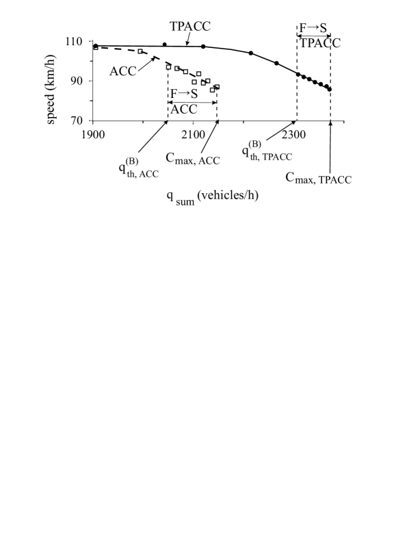
Figure 32: Comparison of traffic stream flow characteristics for free flow on single-lane road with on-ramp bottleneck in mixed traffic with 20$\%$ of autonomous driving vehicles. A part of speed–flow relationship for larger flow rates. Solid curve $``$TPACC” is related to TPACC-vehicles. Dashed curve $``$ACC” is related to classical ACC-vehicles. Stream flow characteristics have been calculated as explained in caption to Fig. 29. In simulations, at $q_{\rm sum}\leq$ 2000 vehicles/h there is no on-ramp inflow ($q_{\rm on}=0$); at $q_{\rm sum}=q_{\rm in}+q_{\rm on}>$ 2000 vehicles/h, the increase in $q_{\rm sum}$ has been achieved through increase in $q_{\rm on}$ at constant $q_{\rm in}=$ 2000 vehicles/h. Simulation parameters of ACC and TPACC are, respectively, the same as those in Fig. 8. Calculated values: $q^{\rm(B)}_{\rm th,\ TPACC}=2308$ and $C_{\rm max,\ TPACC}=2371$ vehicles/h; $q^{\rm(B)}_{\rm th,\ ACC}=2050$ and $C_{\rm max,\ ACC}=2147$ vehicles/h.

We might assume that vehicles implementing TPACC strategy (9) can reduce the overall flow for the traffic stream due to their different use of available space on the road. However, simulations presented in [73] show that no such adverse effect for the traffic stream occurs. Contrarily, rather than reduction of the overall flow through the use of TPACC-vehicles, we have found that TPACC-vehicles increase on average the overall flow (compare values $q^{\rm(B)}_{\rm th,\ TPACC}$, $C_{\rm max,\ TPACC}$ in Fig. 29 with, respectively, these values given in caption to Fig. 32).

In contrast with TPACC-vehicles, we have found that classical ACC-vehicles reduce on average the overall flow in mixed traffic flow (Fig. 32). As explained in Secs. 5–7, this effect of the overall flow reduction caused by classical ACC-vehicles is explained by the occurrence of large local speed disturbances at the bottleneck in mixed traffic flow. The local speed disturbances initiate traffic breakdown in the mixed traffic flow at considerably smaller flow rates in comparison with traffic flow without classical ACC-vehicles. Thus, through the strong effect of autonomous driving vehicles on traffic breakdown at the bottleneck, in simulations we cannot resolve the effect of the different use of available space on the road by TPACC-vehicles and ACC-vehicles on the overall flow.

Thus, we have found that autonomous driving based on the TPACC strategy can increase on average the overall flow for mixed traffic flow. Contrarily to the TPACC strategy, autonomous driving based on the classical ACC strategy decreases on average the overall flow (Figs. 31 and 32).

10 Discussion

10.1 Conclusions

In the article, we have reviewed results of studies of the ACC in the framework of three-phase theory (TPACC) as well as the effect of autonomous driving on traffic breakdown. Additionally, we have presented novel results of the article that have been achieved through a mathematical model for rules of ACC (21)–(25) introduced in this paper. Through the use of this ACC model (21)–(25), we have found the following results:

• In a wide range of the desired time headway to the preceding vehicle classical ACC-vehicle causes a large local speed disturbance at a highway bottleneck. This large disturbance increases the probability of traffic breakdown: Even a single autonomous driving vehicle based on the classical ACC-strategy can provoke traffic breakdown at the bottleneck in mixed traffic flow. Respectively, classical ACC-vehicles decreases the maximum highway capacity.

• At the same chosen flow rate, the longer the desired time headway of the classical ACC-vehicle to the preceding vehicle is, the larger the probability of traffic breakdown caused by a single classical ACC-vehicle at the bottleneck.

• Contrarily to classical ACC-vehicles, in a wide range of headway times TPACC-vehicles can even reduce local speed disturbances at the bottleneck. For this reason, single TPACC-vehicles does not change the probability of traffic breakdown.

We can make the following general conclusions:

1. For the enhancing of future mixed traffic flow, the dynamics of autonomous driving vehicles should learn from some common features of human driving vehicles. Indeed, if the dynamics of the autonomous driving vehicle is qualitatively different from the common dynamic behavior of human driving vehicles, an autonomous driving vehicle might be considered an $``$obstacle” for human driving vehicles in mixed traffic flow. This can reduce traffic safety as well as decrease highway capacity. This explains the necessity of the use of autonomous driving vehicles those dynamics in car-following is familiar for humans. One of the important features of the common dynamic behavior of human driving vehicles found out in empirical data and firstly incorporated in the three-phase traffic theory is an indifference zone in car-following in synchronized flow leading to a two-dimensional (2D) region of synchronized flow states.

2. To find results of the effect of autonomous driving vehicles on mixed traffic flow that are valid for the reality, the dynamics of human driving vehicles in mixed traffic flow must be simulated with a microscopic traffic flow model in the framework of the three-phase theory. Indeed, we have explained that and why if one of the standard traffic flow models for simulations of human driving vehicles is used, then results of a study of the effect of autonomous driving vehicles are invalid for the real world. We use the term $``$standard” for traffic flow models that are related to the state-of-the-art in traffic and transportation research. Examples of standard (classical) traffic flow models can be found in papers, reviews, and books [29, 30, 31, 32, 33, 34, 35, 36, 37, 38, 39, 40, 41, 42, 43, 44, 45, 46, 47, 48, 49, 50, 51, 52]. This criticism on the standard (classical) traffic flow models has been explained in reviews [78, 79, 80, 81, 82, 83, 128].

The advantages of TPACC are associated with the absence of a fixed desired time headway to the preceding vehicle in the TPACC strategy: An TPACC-vehicle exhibits a large indifference zone within the time headway range (13) within which the TPACC-vehicle does not control time headway to the preceding vehicle. As we have explained in this paper, due to the large indifference zone within the time headway range (13), the TPACC-vehicle should not necessarily decelerate as strong as the preceding vehicle when a local short-time speed disturbance appears at a road bottleneck. This dynamic behavior of TPACC-vehicles decreases local speed disturbances in free flow at a road bottleneck. In its turn, the decrease in the amplitude of local speed disturbances at road bottlenecks results in a decrease in the probability of traffic breakdown in the traffic stream.

10.2 About Applicability of Model Results for Future Autonomous Driving in Mixed Traffic Flow

10.2.1 Simple Models of Autonomous Driving Reproducing Features of Mixed Traffic Flow

Although the TPACC model (9) [73] as well as the ACC model (21)–(25) introduced in this paper have allowed us to understand the physics of TPACC-vehicles in mixed traffic flow, the following question can arise: Whether can the simple TPACC model (9) and the ACC model (21)–(25) be applicable for reliable statements about physical features of real mixed traffic flow? To answer this question, we consider firstly some features of the TPACC model (9) that might be seemed at the first glance as non-realistic for real traffic flow.

It seems that TPACC model (9) is mathematically of small incremental value from the pre-existing classical ACC model (4). However, we have above shown that this $``$small incremental mathematical value” exhibits a large physical effect on traffic flow. This large physical effect on traffic flow through the TPACC strategy (9) is associated with the TPACC physical feature mentioned above: Through the indifference zone of TPACC (9), a TPACC-vehicle does not react on the time headway change within the time headway range (13). This dynamic behavior of TPACC-vehicles decreases local speed disturbances in free flow at the bottleneck. The reduction of the local speed disturbances results in a decrease in the breakdown probability in the traffic stream.

This review deals with a subset of the functionality required for autonomous driving, namely longitudinal following a given leader. Other challenges for autonomous driving such as lateral dynamics or sensor-related problems, which are important to satisfy a safety motion of autonomous driving vehicles on multi-lane highways and urban areas (see, e.g., [1, 2, 3, 8, 9, 10, 22]), are not tackled in this review paper. Therefore, a question can arise in what degree results derived for TPACC are related to future autonomous driving.

As mentioned in Sec. 1, in empirical data the qualitative flow-rate dependence of the probability of traffic breakdown at a road bottleneck does not depend on the number of highway lanes (on features of lateral dynamics of vehicles), on the bottleneck type, and on real vehicle technology (during last 30 years vehicle technology was changed considerably, however, qualitative empirical features of traffic breakdown did not change). In accordance with the three-phase theory that explains all known empirical features of traffic breakdown [53, 54, 55], the simple ACC-model and TPACC-model used in the paper reflect dynamic vehicle features that are responsible for traffic breakdown. For this reason, the result of the paper that at the same model parameters classic ACC-vehicles (4) increase the breakdown probability, whereas TPACC-vehicles (9) decrease the breakdown probability proves that the use of indifference zones of the three-phase theory can have benefits for future autonomous driving. This is because contrarily with (4), human driving vehicles do not control time headway within the time headway range (13) [53, 54, 55]. Thus, the TPACC vehicles, which can be considered autonomous driving $``$learning” from empirical human driving behavior, can decrease the breakdown probability.

10.2.2 TPACC as ACC Learning from Driver Behavior

Results of this review allow us to assume that future systems for autonomous driving should be developed whose rules are consistent with those of human driving vehicles. Otherwise, we could expect that autonomous driving vehicles can be considered as $``$obstacles” for drivers. The physics of autonomous driving in the framework of the three-phase theory studied in this paper emphasizes that future autonomous driving should be developed in which both the longitudinal dynamics (TPACC) and lateral dynamics should learn from driver behavior. In particular, the longitudinal and lateral dynamics of autonomous driving vehicles should be consistent with the existence of indifference zones of the three-phase theory [53, 54, 55, 60, 62].

10.2.3 About Simulations of Autonomous Driving in Dangerous Traffic Situations

A question can arise from the choice of the model time step $\tau=$ 1 s in Eqs. (64)–(66) of Appendix B and Eqs. (67)–(69) of Appendix C that have been used for numerical simulations of ACC model (4) and TPACC model (9), respectively. In these models of ACC and TPACC the time step $\tau=$ 1 s determines the safe space gap $g_{\rm safe}=v\tau$ under hypothetical steady state conditions in which all vehicles move at time-independent speed $v$. Contrarily to the ACC model (64)–(66) and the TPACC model (67)–(69), typical ACC controllers in vehicles that on the market have update time intervals $\tau$ of 100 ms or less. Indeed, there may be some very dangerous traffic situations in real traffic in which the safe time headway for an ACC-vehicle is quickly reached and, therefore, the ACC-vehicle must decelerate strongly already after a time interval that is a much shorter than 1 s to avoid the collision with the preceding vehicle. Therefore, to avoid collisions, real ACC-controllers must have update time intervals $\tau$ of 100 ms or less. However, at model time step $\tau=$ 1 s through the choice in the mathematical formulation of the safe speed in Eqs. (64)–(66) of Appendix B and Eqs. (67)–(69) of Appendix C as well as in the model of human driving vehicles (see Secs. A.6 and B of Appendix), collision-less traffic flow is guaranteed in any dangerous traffic situation that can occur in simulations of traffic flow.

In other words, to disclose the physics of TPACC it is sufficient the choice of the update time $\tau=$ 1 s in simulations of TPACC behavior. To explain this, we should note that Eqs. (68), (69) of Appendix C effect on TPACC dynamics only under condition $g_{n}<g_{\rm safe,n}$, i.e., when the space gap becomes smaller than the safe one. This is because the physics of TPACC disclosed in this paper is solely determined by Eq. (67): Under condition $g_{n}\geq g_{\rm safe,n}$, Eqs. (68), (69) do not change TPACC acceleration (deceleration) calculated through Eq. (67). The same conclusion is also valid for the ACC model Eqs. (64)–(66) of Appendix B.

10.3 Can Vehicular Traffic consisting of 100$\%$ Autonomous Vehicles be Real Option in The Future?

In this review paper, we have focused on mixed traffic flow with a small percentage of autonomous driving vehicles. There are the following reasons for this limitation of the study made in this paper. First, in the near future only a very small percentage of autonomous driving vehicles in mixed traffic flow can be expected. Second, we would like to study whether already a single autonomous driving vehicle surrounded by human driving vehicles can effect on traffic breakdown at the bottleneck. Indeed, we have found that already a single autonomous driving vehicle whose dynamics is based on the classical (standard) approach can provoke traffic breakdown at the bottleneck. We have also found that such a deterioration of traffic system does not occur when a autonomous driving vehicle learns from driver behavior in car-following as introduced in the three-phase theory.

Dynamic rules of autonomous driving vehicles can be developed that are totally different from the dynamic behavior of human driving vehicles. In other words, for traffic flow consisting of 100$\%$ of autonomous driving vehicles the dynamic rules of autonomous driving vehicle should not necessarily be consistent with the dynamic behavior of human driving vehicles. One of the consequences is that in traffic flow consisting of 100$\%$ of autonomous driving vehicles highway capacity can be considerably larger in comparison with highway capacity of mixed traffic flow studied in the paper. Therefore, a question can arise: Why does the effect of autonomous driving vehicle on traffic breakdown and capacity of mixed traffic flow studied in this paper is important for future vehicular traffic?

To answer this question, we should discuss whether and when traffic flow consisting of 100$\%$ of autonomous driving vehicles in a traffic network without human driving vehicles could be possible to expect. First, we assume that in the future all vehicles are autonomous driving vehicles only. We could expect that there is at least one reason that might prevent the realization of this case:

• Service costs for autonomous vehicles could be many times larger than those for conventional vehicles driving by humans. Indeed, the check of systems for autonomous driving should be made much frequently than it is needed for the case for a manual driving vehicle. This is because a sudden failure of a system for autonomous driving in a vehicle can lead to an accident with catastrophic consequences for both passengers of the autonomous driving vehicle and passengers of several other following vehicles in traffic flow. Such a frequent check of systems for autonomous driving could lead to enormous service costs that could be paid by only a (small) part of vehicle owners.

If in the future some of the vehicles moving in traffic networks are manual driving ones, then we can assume that two independent from each other traffic networks might be developed: (i) One network is dedicated to autonomous driving vehicles only. (ii) Another network is dedicated to human driving vehicles only. We could expect that there is at least one reason that might prevent the realization of this case:

• Extremely high costs for the development of two independent from each other traffic networks.

It is clear that the organization of high-speed highway lanes, or some separated roads, or else a part of a traffic network dedicated to connected autonomous vehicles is possible as, for example, suggested in [175, 176, 177, 178, 179, 180]. In this case, in another network part in which human driving vehicles can move, mixed traffic flow is realized. Therefore, it could be expected that mixed traffic flow will remain the reality also for future vehicular traffic.

11 Future Directions

In this review paper, we have made a comparison of the effect of classical ACC-vehicles and TPACC-vehicles on the probability of traffic breakdown at a road bottleneck in mixed traffic flow. In this scenario of the application of autonomous driving vehicles, rather than only some specific values of TPACC and ACC parameters as made in [73, 74] we have considered a wide range of headway times to demonstrate that the TPACC strategy can exhibit advantages in comparison with the classical ACC. Moreover, through the use of ACC model (21)–(25) we could understand the physical difference between classical ACC strategy and TPACC in more details.

However, a change in other parameters of ACC might give different results. Additionally, incorporating cooperative merging between ACC vehicles could reduce the tendency to initiate breakdown at highway bottlenecks. We believe that related detailed studies of the TPACC model, which are out of the scope of this review, will be a very interesting task of future investigations of the physics of autonomous driving.

Appendix A Kerner-Klenov Microscopic Stochastic Traffic Flow Model

In this Appendix, we make explanations of the Kerner-Klenov stochastic microscopic three-phase model for human driving vehicles [75, 76, 77] and model parameters used for simulations of mixed traffic flow presented in the main text.

A.1 Update Rules of Vehicle Motion

In a discrete model version of the Kerner-Klenov stochastic microscopic three-phase model used in all simulations presentred in the main text, rather than the continuum space co-ordinate [75], a discretized space co-ordinate with a small enough value of the discretization space interval $\delta x$ is used [77]. Consequently, the vehicle speed and acceleration (deceleration) discretization intervals are $\delta v=\delta x/\tau$ and $\delta a=\delta v/\tau$, respectively, where $\tau$ is time step. Because in the discrete model version discrete (and dimensionless) values of space coordinate, speed and acceleration are used, which are measured respectively in values $\delta x$, $\delta v$ and $\delta a$, and time is measured in values of $\tau$, value $\tau$ in all formulas is assumed below to be the dimensionless value $\tau=1$. In the discrete model version used for all simulations, the discretization cell $\delta x=$ 0.01 m is used.

A choice of $\delta x=0.01$ m made in the model determines the accuracy of vehicle speed calculations in comparison with the initial continuum in space stochastic model of [75]. We have found that the discrete model exhibits similar characteristics of phase transitions and resulting congested patterns at highway bottlenecks as those in the continuum model at $\delta x$ that satisfies the conditions

$$\delta x/\tau^{2}\ll b,\ a,\ a^{\rm(a)},\ a^{\rm(b)},\ a^{\rm(0)},$$ (28)

where model parameters for driver deceleration and acceleration $b$, $a$, $a^{\rm(a)}$, $a^{\rm(b)}$, $a^{\rm(0)}$ will be explained below.

Update rules of vehicle motion in the discrete model for identical drivers and identical vehicles moving in a road lane are as follows [77]:

$$v_{n+1}=\max(0,\min({v_{\rm free},\tilde{v}_{n+1}+\xi_{n},v_{n}+a\tau,v_{{\rm s},n}})),$$ (29)

$$x_{n+1}=x_{n}+v_{n+1}\tau,$$ (30)

where the index $n$ corresponds to the discrete time $t_{\rm n}=\tau n,\ n=0,1,...$; $v_{n}$ is the vehicle speed at time step $n$, $a$ is the maximum acceleration, $\tilde{v}_{n}$ is the vehicle speed without speed fluctuations $\xi_{n}$:

$$\tilde{v}_{n+1}=\min(v_{\rm free},v_{{\rm s},n},v_{{\rm c},n}),$$ (31)

$$v_{{\rm c},n}=\left\{\begin{array}[]{ll}v_{n}+\Delta_{n}&\textrm{at $g_{n}\leq G_{n}$}\\ v_{n}+a_{n}\tau&\textrm{at $g_{n}>G_{n}$},\\ \end{array}\right.$$ (32)

$$\Delta_{n}=\max(-b_{n}\tau,\min(a_{n}\tau,\ v_{\ell,n}-v_{n})),$$ (33)

$$g_{n}=x_{\ell,n}-x_{n}-d,$$ (34)

the subscript $\ell$ marks variables related to the preceding vehicle, $v_{{\rm s},n}$ is a safe speed at time step $n$, $v_{\rm free}$ is the free flow speed in free flow, $\xi_{n}$ describes speed fluctuations; $g_{n}$ is a space gap between two vehicles following each other; $G_{n}$ is the synchronization space gap; all vehicles have the same length $d$. The vehicle length $d$ includes the mean space gap between vehicles that are in a standstill within a wide moving jam. Values $a_{n}\geq 0$ and $b_{n}\geq 0$ in (32), (33) restrict changes in speed per time step when the vehicle accelerates or adjusts the speed to that of the preceding vehicle.

A.2 Synchronization Space Gap and Hypothetical Steady States of Synchronized Flow

Equations (32), (33) describe the adaptation of the vehicle speed to the speed of the preceding vehicle, i.e., the speed adaptation effect in synchronized flow. This vehicle speed adaptation takes place within the synchronization gap $G_{n}$: At

$$g_{n}\leq G_{n}$$ (35)

the vehicle tends to adjust its speed to the speed of the preceding vehicle. This means that the vehicle decelerates if $v_{n}>v_{\ell,n}$, and accelerates if $v_{n}<v_{\ell,n}$.

In (32), the synchronization gap $G_{n}$ depends on the vehicle speed $v_{n}$ and on the speed of the preceding vehicle $v_{\ell,n}$:

$$G_{n}=G(v_{n},v_{\ell,n}),$$ (36)

$$G(u,w)=\max(0,\lfloor k\tau u+a^{-1}u(u-w)\rfloor),$$ (37)

where $k>1$ is constant; $\lfloor{z}\rfloor$ denotes the integer part of $z$.

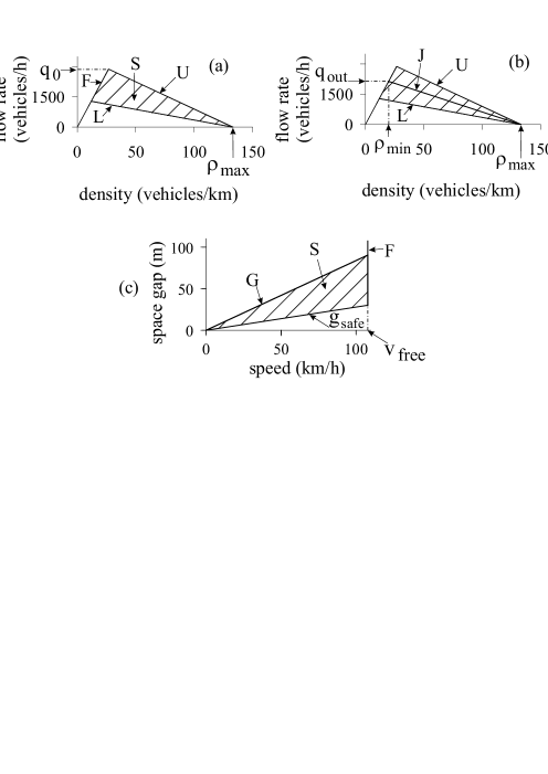
Figure 33: Steady speed states for the Kerner-Klenov traffic flow model in the flow–density (a, b) and in the space-gap–speed planes (c). In (a, b), $L$ and $U$ are, respectively, lower and upper boundaries of 2D-regions of steady states of synchronized flow. In (b), J is the line $J$ whose slope is equal to the characteristic mean velocity $v_{\rm g}$ of a wide moving jam; in the flow–density plane, the line $J$ represents the propagation of the downstream front of the wide moving jam with time-independent velocity $v_{\rm g}$. F – free flow, S – synchronized flow.

The speed adaptation effect within the synchronization distance is related to the hypothesis of the three-phase theory: Hypothetical steady states of synchronized flow cover a 2D region in the flow–density (Fig. 33 (a)). Boundaries $F$, $L$, and $U$ of this 2D-region shown in Fig. 33 (a) are, respectively, associated with the free flow speed in free flow, a synchronization space gap $G$, and a safe space gap $g_{\rm safe}$. A speed-function of the safe space gap $g_{\rm safe}(v)$ is found from the equation

$$v=v_{\rm s}(g_{\rm safe},\ v).$$ (38)

Respectively, as for the continuum model (see Sec. 16.3 of the book [53]), for the discrete model hypothetical steady states of synchronized flow cover a 2D-region in the flow–density plane (Fig. 33 (a, b)). However, because the speed $v$ and space gap $g$ are integer in the discrete model, the steady states do not form a continuum in the flow–density plane as they do in the continuum model. The inequalities

$$v\leq v_{\rm free},\quad g\leq G(v,\ v),\quad g\geq g_{\rm safe}(v),$$ (39)

define a 2D-region in the space-gap–speed plane (Fig. 33 (c)) in which the hypothetical steady states exist for the discrete model, when all model fluctuations are neglected.

In (39), we have taken into account that in the hypothetical steady states of synchronized flow vehicle speeds and space gaps are assumed to be time-independent and the speed of each of the vehicles is equal to the speed of the associated preceding vehicle: $v=v_{\ell}$. However, due to model fluctuations, steady states of synchronized flow are destroyed, i.e., they do not exist in simulations; this explains the term $``$hypothetical” steady states of synchronized flow. Therefore, rather than steady states some non-homogeneous in space and time traffic states occur. In other words, steady states are related to a hypothetical model fluctuation-less limit of homogeneous in space and time vehicle motion that does not realized in real simulations. Driver time delays are described through model fluctuations. Therefore, any application of the Kerner-Klenov stochastic microscopic three-phase traffic flow model without model fluctuations has no sense. In other words, for the description of real spatiotemporal traffic flow phenomena, model speed fluctuations incorporated in this model are needed.

A.3 Model Speed Fluctuations

In the model, random vehicle deceleration and acceleration are applied depending on whether the vehicle decelerates or accelerates, or else maintains its speed:

$$\xi_{n}=\left\{\begin{array}[]{ll}\xi_{\rm a}&\textrm{if $S_{n+1}=1$}\\ -\xi_{\rm b}&\textrm{if $S_{n+1}=-1$}\\ \xi^{(0)}&\textrm{if $S_{n+1}=0$}.\end{array}\right.$$ (40)

State of vehicle motion $S_{n+1}$ in (40) is determined by formula

$$S_{n+1}=\left\{\begin{array}[]{ll}-1&\textrm{if $\tilde{v}_{n+1}<v_{n}$}\\ 1&\textrm{if $\tilde{v}_{n+1}>v_{n}$}\\ 0&\textrm{if $\tilde{v}_{n+1}=v_{n}$}.\end{array}\right.$$ (41)

In (40), $\xi_{\rm b}$, $\xi^{(0)}$, and $\xi_{\rm a}$ are random sources for deceleration and acceleration that are as follows:

$$\xi_{\rm b}=a^{(\rm b)}\tau\Theta(p_{\rm b}-r),$$ (42)

$$\xi^{(0)}=a^{(0)}\tau\left\{\begin{array}[]{ll}-1&\textrm{if $r<p^{(0)}$}\\ 1&\textrm{if $p^{(0)}\leq r<2p^{(0)}$}\quad{\rm and}\ v_{n}>0\\ 0&\textrm{otherwise},\end{array}\right.$$ (43)

$$\xi_{\rm a}=a^{(\rm a)}\tau\Theta(p_{\rm a}-r),$$ (44)

$p_{\rm b}$ is probability of random vehicle deceleration, $p_{\rm a}$ is probability of random vehicle acceleration, $p^{(0)}$ and $a^{(0)}\leq a$ are constants, $r={\rm rand(0,1)}$, $\Theta(z)=0$ at $z<0$ and $\Theta(z)=1$ at $z\geq 0$, $a^{(\rm a)}$ and $a^{(\rm b)}$ are model parameters (see Table 1), which in some applications can be chosen as speed functions $a^{(\rm a)}=a^{(\rm a)}(v_{n})$ and $a^{(\rm b)}=a^{(\rm b)}(v_{n})$.

A.4 Stochastic Time Delays of Acceleration and Deceleration

To simulate time delays either in vehicle acceleration or in vehicle deceleration, $a_{n}$ and $b_{n}$ in (33) are taken as the following stochastic functions

$$a_{n}=a\Theta(P_{\rm 0}-r_{\rm 1}),$$ (45)

$$b_{n}=a\Theta(P_{\rm 1}-r_{\rm 1}),$$ (46)

$$P_{\rm 0}=\left\{\begin{array}[]{ll}p_{\rm 0}&\textrm{if $S_{n}\neq 1$}\\ 1&\textrm{if $S_{n}=1$},\end{array}\right.$$ (47)

$$P_{\rm 1}=\left\{\begin{array}[]{ll}p_{\rm 1}&\textrm{if $S_{n}\neq-1$}\\ p_{\rm 2}&\textrm{if $S_{n}=-1$},\end{array}\right.$$ (48)

$r_{1}={\rm rand}(0,1)$, $p_{\rm 1}$ is constant, $p_{\rm 0}=p_{\rm 0}(v_{n})$ and $p_{\rm 2}=p_{\rm 2}(v_{n})$ are speed functions (see Table 1).

A.5 Simulations of Slow-to-Start Rule

In the model, simulations of the well-known effect of the driver time delay in acceleration at the downstream front of synchronized flow or a wide moving jam known as a slow-to-start rule [181, 182] are made as a collective effect through the use of Eqs. (32), (33), and a random value of vehicle acceleration (45). Eq. (45) with $P_{0}=p_{0}<1$ is applied only if the vehicle did not accelerate at the former time step ($S_{n}\neq 1$); in the latter case, a vehicle accelerates with some probability $p_{0}$ that depends on the speed $v_{n}$; otherwise $P_{\rm 0}=1$ (see formula (47)).

The mean time delay in vehicle acceleration is equal to

$$\tau^{\rm(acc)}_{\rm del}(v_{n})=\frac{\tau}{p_{0}(v_{n})}.$$ (49)

From formula (49), it follows that the mean time delay in vehicle acceleration from a standstill within a wide moving jam (i.e., when in formula (49) the speed $v_{n}=0$) is equal to

$$\tau^{\rm(acc)}_{\rm del}(0)=\frac{\tau}{p_{0}(0)}.$$ (50)

The mean time delay in vehicle acceleration from a standstill within a wide moving jam determines the parameters of the line $J$ in the flow–density plane (Fig. 33 (b)).

Probability $p_{\rm 0}(v_{n})$ in (47) is chosen to be an increasing speed function (see Table 1). Because the speed within synchronized flow is larger than zero, the mean time delay in vehicle acceleration at the downstream front of synchronized flow that we denote by

$$\tau^{\rm(acc)}_{\rm del,\ syn}=\tau^{\rm(acc)}_{\rm del}(v_{n}),\quad v_{n}>0$$ (51)

is shorter than the mean time delay in vehicle acceleration at the downstream front of the wide moving jam $\tau^{\rm(acc)}_{\rm del}(0)$:

$$\tau^{\rm(acc)}_{\rm del,\ syn}<\tau^{\rm(acc)}_{\rm del}(0).$$ (52)

A.6 Safe Speed

In the model, the safe speed $v_{{\rm s},n}$ in (29) is chosen in the form

$$v_{{\rm s},n}=\min{(v^{\rm(safe)}_{n},g_{n}/\tau+v^{\rm(a)}_{\ell})},$$ (53)

$v^{\rm(a)}_{\ell}$ is an $``$anticipation” speed of the preceding vehicle that will be considered below, the function

$$v^{\rm(safe)}_{n}=\lfloor v^{\rm(safe)}(g_{n},\ v_{\ell,n})\rfloor$$ (54)

in (53) is related to the safe speed $v^{\rm(safe)}(g_{n},\ v_{\ell,n})$ in the model by Krauß et al. [184], which is a solution of the Gipps’s equation [183]

$$v^{\rm(safe)}\tau+X_{\rm d}(v^{\rm(safe)})=g_{n}+X_{\rm d}(v_{\ell,n}),$$ (55)

where $X_{\rm d}(u)$ is the braking distance that should be passed by the vehicle moving first with the speed $u$ before the vehicle can come to a stop.

The condition (55) enables us to find the safe speed $v^{\rm(safe)}$ as a function of the space gap $g_{n}$ and speed $v_{\ell,n}$ provided $X_{\rm d}(u)$ is a known function. In the case when the vehicle brakes with a constant deceleration $b$, the change in the vehicle speed for each time step is $-b\tau$ except the last time step before the vehicle comes to a stop. At the last time step, the vehicle decreases its speed at the value $b\tau\beta$, where $\beta$ is a fractional part of $u/b\tau$. According to formula (30) for the displacement of the vehicle for one time step, the braking distance $X_{\rm d}(u)$ is [184]

$$X_{\rm d}(u)=\tau\big{(}u-b\tau+u-2b\tau+...+\beta b\tau\big{)}.$$ (56)

From (56), it follows [184]

$$X_{\rm d}(u)=b\tau^{2}\bigg{(}\alpha\beta+\frac{\alpha(\alpha-1)}{2}\bigg{)},$$ (57)

$\alpha=\lfloor u/b\tau\rfloor$ is an integer part of $u/b\tau$.

The safe speed $v^{\rm(safe)}$ as a solution of equation (55) at the distance $X_{\rm d}(u)$ given by (57) has been found by Krauß et al. [184]

$$v^{\rm(safe)}(g_{n},v_{\ell,n})=b\tau(\alpha_{\rm safe}+\beta_{\rm safe}),$$ (58)

where

$$\alpha_{\rm safe}=\left\lfloor{\sqrt{2\frac{X_{\rm d}(v_{\ell,n})+g_{n}}{b\tau^{2}}+\frac{1}{4}}-\frac{1}{2}}\right\rfloor,$$ (59)

$$\beta_{\rm safe}=\frac{X_{\rm d}(v_{\ell,n})+g_{n}}{(\alpha_{\rm safe}+1)b\tau^{2}}-\frac{\alpha_{\rm safe}}{2}.$$ (60)

The safe speed in the model by Krauß et al. [184, 185] provides collision-less motion of vehicles if the time gap $g_{n}/v_{n}$ between two vehicles is greater than or equal to the time step $\tau$, i.e., if $g_{n}\geq v_{n}\tau$ [185]. In the model, it is assumed that in some cases, mainly due to lane changing or merging of vehicles onto the main road within the merging region of bottlenecks, the space gap $g_{n}$ can become less than $v_{n}\tau$. In these critical situations, the collision-less motion of vehicles in the model is a result of the second term in (53) in which some prediction ($v^{\rm(a)}_{\ell}$) of the speed of the preceding vehicle at the next time step is used. The related $``$anticipation” speed $v^{\rm(a)}_{\ell}$ at the next time step is given by formula

$$v^{\rm(a)}_{\ell}=\max(0,\min(v^{\rm(safe)}_{\ell,n},v_{\ell,n},g_{\ell,n}/\tau)-a\tau),$$ (61)

where $v^{\rm(safe)}_{\ell,n}$ is the safe speed (54), (58)–(60) for the preceding vehicle, $g_{\ell,n}$ is the space gap in front of the preceding vehicle. Simulations have shown that formulas (53), (54), (58)–(61) lead to collision-less vehicle motion over a wide range of parameters of the merging region of on-ramp bottlenecks (Appendix E).

In hypothetical steady states of traffic flow (Fig. 33 (a)), the safe space gap $g_{\rm safe}$ is determined from condition $v=v_{\rm s}$. In accordance with Eqs. (53)–(55), at a given $v$ in steady traffic states $v=v_{\ell}$ for the safe speed $v_{\rm s}$ we get

$$v_{\rm s}=g_{\rm safe}/\tau,$$ (62)

and, therefore,

$$g_{\rm safe}=v\tau.$$ (63)

Thus, for hypothetical steady states of traffic flow $\tau_{\rm safe}=\tau=1$ s.

Table 1: Model parameters of vehicle motion in road lane used in simulations of the main text

$\tau_{\rm safe}=\tau=$ 1 s, $d=7.5\ \rm m/\delta x$,
$\delta x=$ 0.01 m, $\delta v=0.01\ {\rm ms^{-1}}$, $\delta a=0.01\ {\rm ms^{-2}}$,
$v_{\rm free}=30\ {\rm ms^{-1}}/\delta v$, $b=1\ {\rm ms^{-2}}/\delta a$, $a=$ 0.5 ${\rm ms^{-2}}/\delta a$,
$k=$ 3, $p_{1}=$ 0.3, $p_{b}=0.1$, $p_{a}=0.17$, $p^{(0)}=0.005$,
$p_{\rm 0}(v_{n})=0.575+0.125\min{(1,v_{n}/v_{01})}$,
$p_{\rm 2}(v_{n})=0.48+0.32\Theta{(v_{n}-v_{21})}$,
$v_{01}=10\ {\rm ms^{-1}}/\delta v$, $v_{21}=15\ {\rm ms^{-1}}/\delta v$,
$a^{(0)}=0.2a$, $a^{(\rm a)}=a^{(\rm b)}=a$.

In [55] it has been shown that the Kerner-Klenov model (29)–(34), (36), (37), (40)–(48), (53), (54), (58)–(61) is a Markov chain: At time step $n+1$, values of model variables $v_{n+1}$, $x_{n+1}$, and $S_{n+1}$ are calculated based only on their values $v_{n}$, $x_{n}$, and $S_{n}$ at step $n$.

It should be noted that after the Kerner-Klenov car-following model with indifference zones in car-following based on the three-phase theory (dashed region in Fig. 7) has been introduced [75] (as mentioned, in this review article a discrete version of this model of Ref. [77] has been used), a number of different traffic flow models incorporating some of the hypotheses of the three-phase theory have been developed and many results with the use of these models have been found (e.g., [23, 24, 76, 82, 84, 85, 86], [186, 187, 188, 189, 190, 191, 192, 193], [194, 195, 196, 197, 198], [199, 200, 201, 202], [203, 204, 205, 206, 207, 208, 209, 210, 211], [212, 213, 214, 215, 216, 217, 218], [219, 220, 221, 222, 223, 224], [225, 226, 227, 228, 229, 230], [231, 232, 233, 234, 235, 236], [237, 238, 239, 240, 241, 242, 243, 244, 245]). A review of some of these models that are related to the class of cellular automation models has been recently done by Tian et al. [246].

Appendix B Discrete Version of Classical ACC Model

In simulations of the classical ACC-model (4), as in the model of human driving vehicles (Appendix A.1) we use the discrete time $t=n\tau$, where $n=0,1,2,..$; $\tau=$1 s is time step. Therefore, the space gap to the preceding vehicle is equal to $g_{n}=x_{\ell,n}-x_{n}-d$ and the relative speed is given by $\Delta v_{n}=v_{\ell,n}-v_{n}$, where $x_{n}$ and $v_{n}$ are coordinate and speed of the ACC-vehicle, $x_{\ell,n}$ and $v_{\ell,n}$ are coordinate and speed of the preceding vehicle, $d$ is the vehicle length that is assumed the same one for autonomous driving and human driving vehicles. Correspondingly, the classical model of the dynamics of ACC-vehicle (4) can be rewritten as follows [83, 55]:

$$a^{\rm(ACC)}_{n}=K_{1}(g_{n}-v_{n}\tau^{\rm(ACC)}_{\rm d})+K_{2}(v_{\ell,n}-v_{n}).$$ (64)

The ACC vehicles move in accordance with Eq. (64) where, in addition, the following formulas are used:

$$v^{\rm(ACC)}_{{\rm c},n}=v_{n}+\tau\max(-b_{\rm max},\min(\lfloor a^{\rm(ACC)}_{n}\rfloor,a_{\rm max})),$$ (65)

$$v_{n+1}=\max(0,\min({v_{\rm free},v^{\rm(ACC)}_{{\rm c},n},v_{{\rm s},n}})),$$ (66)

$\lfloor z\rfloor$ denotes the integer part of $z$. Through the use of formula (65), acceleration and deceleration of the ACC vehicles are limited by some maximum acceleration $a_{\rm max}$ and maximum deceleration $b_{\rm max}$, respectively. Owing to the formula (66), the speed of the ACC vehicle $v_{n+1}$ at time step $n+1$ is limited by the maximum speed in free flow $v_{\rm free}$ and by the safe speed $v_{{\rm s},n}$ to avoid collisions between vehicles. The maximum speed in free flow $v_{\rm free}$ and the safe speed $v_{{\rm s},n}$ are chosen, respectively, the same as those in the microscopic model of human driving vehicles (Appendix A). It should be noted that the model of ACC-vehicle merging from the on-ramp onto the main road is similar to that for human driving vehicles (see Appendix E.2).

Simulations show that the use of the safe speed in formula (66) does not influence on the dynamics of the ACC vehicles (4) in free flow outside the bottleneck. However, due to vehicle merging from the on-ramp onto the main road, time headway of the vehicle to the preceding vehicle can be considerably smaller than $\tau^{\rm(ACC)}_{\rm d}$. Therefore, formula (66) allows us to avoid collisions of the ACC vehicle with the preceding vehicle in such dangerous situations. Moreover, very small values of time headway can occur in congested traffic; formula (66) prevents vehicle collisions in these cases also.

Appendix C Discrete Version of TPACC Model

The model for human driving vehicles [75, 76, 77] used in all simulations is discrete in time (Appendix A). Therefore, we simulate TPACC-model (9) with discrete time $t_{\rm n}=\tau n,\ n=0,1,...$. Respectively, TPACC-model (9) should be rewritten as follows:

$$a^{\rm(TPACC)}_{n}=\left\{\begin{array}[]{ll}K_{\rm\Delta v}(v_{\ell,n}-v_{n})&\textrm{at $g_{n}\leq G_{n}$}\\ K_{1}(g_{n}-v_{n}\tau_{\rm p})+K_{2}(v_{\ell,n}-v_{n})&\textrm{at $g_{n}>G_{n}$},\\ \end{array}\right.$$ (67)

where $G_{n}=v_{n}\tau_{\rm G}$ and $\tau_{\rm p}<\tau_{\rm G}$.

C.1 Safety Conditions

When $g_{n}<g_{\rm safe,n}$, the TPACC-vehicle should move in accordance with some safety conditions to avoid collisions between vehicles (Fig. 7). A collision-free TPACC-vehicle motion is described as made in [83] for the classical model of ACC: (68) (69)

$$v^{\rm(TPACC)}_{{\rm c},n}=v_{n}+\tau\max(-b_{\rm max},\min(\lfloor a^{\rm(TPACC)}_{n}\rfloor,a_{\rm max})),$$ (68)

$$v_{n+1}=\max(0,\min({v_{\rm free},v^{\rm(TPACC)}_{{\rm c},n},v_{{\rm s},n}})),$$ (69)

where the TPACC acceleration and deceleration are limited by $a_{\rm max}$ and $b_{\rm max}$, respectively; the speed $v_{n+1}$ (69) at time step $n+1$ is limited by the maximum speed $v_{\rm free}$ and by the safe speed $v_{{\rm s},n}$ that have been chosen, respectively, the same as those in the model of human driving vehicles; $\lfloor z\rfloor$ denotes the integer part of $z$.

C.2 $``$Indifference Zone” in Car-Following

In accordance with Eq. (69), condition $v^{\rm(TPACC)}_{{\rm c},n}\leq v_{{\rm s},n}$ is equivalent to condition $g_{n}\geq g_{\rm safe,n}$. Under this condition, from the TPACC model (67)–(69) it follows that when time headway $\tau^{\rm(net)}_{n}=g_{n}/v_{n}$ of the TPACC-vehicle to the preceding vehicle is within the range

$$\tau_{{\rm safe},n}\leq\tau^{\rm(net)}_{n}\leq\tau_{\rm G},$$ (70)

the acceleration (deceleration) of the TPACC-vehicle does not depend on time headway. In (70),

$$\tau_{{\rm safe},n}=g_{{\rm safe},n}/v_{n}$$ (71)

is a safe time headway and it is assumed that $v{{}_{n}}>0$. The safe gap $g_{{\rm safe},n}$ in formula (71) is found as follows. The value $g_{{\rm safe},n}$ is found as a solution of equation

$$v^{\rm(TPACC)}_{{\rm c},n}=v_{{\rm safe}}(g_{{\rm safe},n},v_{\ell,n},v^{(\rm a)}_{\ell}),$$ (72)

in which the value $v^{\rm(TPACC)}_{{\rm c},n}$ is given by (68) and the function $v_{{\rm safe}}(g_{{\rm safe},n},v_{\ell,n},v^{(\rm a)}_{\ell})$ is determined by formula (53) where $g_{n}$ is replaced by $g_{{\rm safe},n}$.

In accordance with (70), for the TPACC model (67)–(69) there is no fixed desired time headway to the preceding vehicle (Fig. 7). This means that in the TPACC model (67)–(69) there is $``$indifference zone” in the choice of time headway in car-following. This is in contrast with the classical ACC model (4) for which there is a fixed desired time headway in car-following. It should be noted that formula (70) for the indifference zone in time headway of TPACC is a discrete version of formula (13) for the indifference zone in time headway of TPACC discussed in the main text.

C.3 Operating Points

From formula for the safe speed $v_{{\rm s},n}$ in (69) that is given in Appendix A.6, we find that the safe time headway $\tau_{{\rm safe},n}$ in (13) for the operating points of TPACC model (67)–(69) is a constant value that is equal to $\tau_{\rm safe}=\tau=$1 s. In operating points of TPACC model (67)–(69), $a^{\rm(TPACC)}=0$; respectively, $v=v_{\ell}$, $g_{\rm safe}(v)\leq g\leq G(v)$, and $v=v_{\rm free}$ at $g>G(v)$, where $g_{\rm safe}(v)=v\tau$, $G(v)=v\tau_{\rm G}$. The operating points of the TPACC model (67)–(69) cover a 2D-region in the space-gap–speed plane (dashed 2D-region in Fig. 34 (a)). The inequalities $v\leq v_{\rm free}$, $g\leq G(v)$, and $g\geq g_{\rm safe}(v)$ define a 2D-region in the space-gap–speed plane (Fig. 34 (a)) in which the operating points exist for the discrete version of TPACC model (67)–(69).

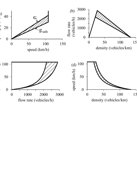
Figure 34: Operating points of TPACC model (67)–(69) presented in the space-gap–speed (a), flow–density (b), speed–flow (c), and speed–density (c) planes. Model parameters $\tau_{\rm G}=$1.4 s, $\tau_{\rm p}=$1.3 s, $\tau_{\rm safe}=$1 s, $v_{\rm free}=30$m/s (108 km/h), vehicle length (including the mean space gap between vehicles stopped within a wide moving jam) $d=$7.5 m.

It should be noted that the speed $v$ and space gap $g$ are integer in the discrete version of TPACC model (67)–(69). Therefore, the operating points do not form a continuum in the space-gap–speed plane as they do in the continuum version of TPACC model (9).

From Fig. 34, we can see that under conditions $g_{\rm safe}(v)\leq g\leq G(v)$ for each given speed $v>0$ of TPACC there is no fixed time headway to the preceding vehicle in operating points of the TPACC model (dashed 2D-regions in Fig. 34), as explained in Sec. 4 (Fig. 7).

The discretization interval of TPACC acceleration (deceleration) made in TPACC model (67)–(69) is chosen to be an extremely small value that is equal to $\delta a=$0.01 ${\rm m/s^{2}}$ (see Appendix A). Therefore, the maximum value of a small round down of $a^{\rm(TPACC)}_{n}$ in Eqs. (68), (69) through the application of the floor operator $\lfloor a^{\rm(TPACC)}_{n}\rfloor$ is less than 0.01 ${\rm m/s^{2}}$ and it is, therefore, negligible. We have tested that no conclusions about physical features of TPACC dynamic behavior have been changed, when the continuum in space model of human driving vehicles of Ref. [76] and, respectively, the continuum in space TPACC model version (without the the floor operator) is used (the reason for the use of the discrete in space model for human driving vehicles of Ref. [77] that leads to Eqs. (68), (69) has been explained in [77] as well as in Appendix A of the book [55]).

Simulations show that the use of the safe speed in formula (69) does not influence on the dynamics of the TPACC vehicles (67) in free flow outside the bottleneck. However, formula (69) allows us to avoid collisions of the TPACC vehicle with the preceding vehicle in dangerous situations that can occur at the bottleneck as well as in congested traffic.

Appendix D Model of ACC with Combination of Dynamic Features of Classical ACC and TPACC

The ACC-acceleration $a^{\rm(C)}_{n}$ in a discrete in time version of the model of ACC (21)–(25) of Sec. 7 reads as follows:

$$a^{\rm(C)}_{n}=\left\{\begin{array}[]{ll}\tilde{a}^{\rm(C)}_{n}&\textrm{at $g_{n}\leq G^{\rm(C)}_{n}$,}\\ a^{\rm(ACC)}_{n}&\textrm{at $g_{n}>G^{\rm(C)}_{n}$},\\ \end{array}\right.$$ (75)

where

$$\tilde{a}^{\rm(C)}_{n}=a^{\rm(2D)}_{n}(1-p^{\rm(C)})+a^{\rm(ACC)}_{n}p^{\rm(C)},$$ (76)

$$a^{\rm(2D)}_{n}=K_{\rm\Delta v}\Delta v_{n},$$ (77)

$$a^{\rm(ACC)}_{n}=K_{1}(g_{n}-v_{n}\tau_{\rm p})+K_{2}\Delta v_{n},$$ (78)

$$G^{\rm(C)}_{n}=G_{n}(1-p^{\rm(C)})+v_{n}\tau_{\rm p}p^{\rm(C)}.$$ (79)

When $g_{n}<g_{\rm safe,n}$, the ACC-vehicle (75)–(79) should move in accordance with some safety conditions to avoid collisions between vehicles. A collision-free ACC-vehicle motion is described as made for the classical model of ACC:

$$v_{n+1}=\max(0,\min({v_{\rm free},v^{\rm(C)}_{{\rm c},n},v_{{\rm s},n}})).$$ (80)

where

$$v^{\rm(C)}_{{\rm c},n}=v_{n}+\tau\max(-b_{\rm max},\min(\lfloor a^{\rm(C)}_{n}\rfloor,a_{\rm max})).$$ (81)

Appendix E Model of On-Ramp Bottleneck

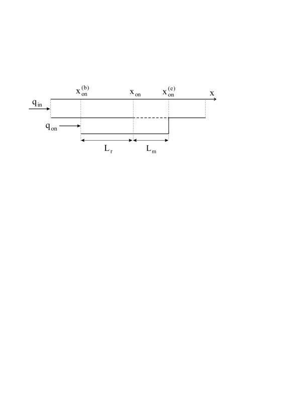
Figure 35: Model of on-ramp bottleneck on single-lane road.

An on-ramp bottleneck consists of two parts (Fig. 35):

(i)

The merging region of length $L_{\rm m}$ where vehicle can merge onto the main road from the on-ramp lane.

(ii)

A part of the on-ramp lane of length $L_{\rm r}$ upstream of the merging region where vehicles move in accordance with the model of Appendix A. The maximal speed of vehicles is $v_{\rm free}=v_{\rm free\ on}$.

At the beginning of the on-ramp lane ($x=x^{\rm(b)}_{\rm on}$) the flow rate to the on-ramp $q_{\rm on}$ is given through boundary conditions that are the same as those that determine the flow rate $q_{\rm in}$ at the beginning of the main road (see Appendix F below).

E.1 Model of Vehicle Merging at Bottleneck

E.1.1 Vehicle Speed Adaptation withing Merging Region of Bottleneck

For the on-ramp bottleneck, when a vehicle is within the merging region of the bottleneck, the vehicle takes into account the space gaps to the preceding vehicles and their speeds both in the current and target lanes. Respectively, instead of formula (32), in (31) for the speed $v_{{\rm c},n}$ the following formula is used:

$$v_{{\rm c},n}=\left\{\begin{array}[]{ll}v_{n}+\Delta^{+}_{n}&\textrm{at $g^{+}_{n}\leq G(v_{n},\hat{v}^{+}_{n})$}\\ v_{n}+a_{n}\tau&\textrm{at $g^{+}_{n}>G(v_{n},\hat{v}^{+}_{n})$},\\ \end{array}\right.$$ (82)

$$\Delta^{+}_{n}=\max(-b_{n}\tau,\min(a_{n}\tau,\ \hat{v}^{+}_{n}-v_{n})),$$ (83)

$$\hat{v}^{+}_{n}=\max(0,\min(v_{\rm free},\ v^{+}_{n}+\Delta v^{(2)}_{r})),$$ (84)

$\Delta v^{(2)}_{r}$ is constant (see Table 2).

Superscripts $+$ and $-$ in variables, parameters, and functions denote the preceding vehicle and the trailing vehicle in the $``$target” (neighboring) lane, respectively. The target lane is the lane into which the vehicle wants to change.

The safe speed $v_{{\rm s},n}$ in (29), (31) for the vehicle that is the closest one to the end of the merging region is chosen in the form

$$v_{{\rm s},n}=\lfloor v^{\rm(safe)}(x^{\rm(e)}_{\rm on}-x_{n},\ 0)\rfloor$$ (85)

(see Table 2).

E.1.2 Safety Conditions for Vehicle Merging

Vehicle merging at the bottleneck occurs, when safety conditions ($\ast$) or safety conditions ($\ast\ast$) are satisfied.

Safety conditions ($\ast$) are as follows:

$$\begin{array}[]{ll}g^{+}_{n}>\min(\hat{v}_{n}\tau,\ G(\hat{v}_{n},v^{+}_{n})),\\ g^{-}_{n}>\min(v^{-}_{n}\tau,\ G(v^{-}_{n},\hat{v}_{n})),\end{array}$$ (86)

$$\hat{v}_{n}=\min(v^{+}_{n},\ v_{n}+\Delta v^{(1)}_{r}),$$ (87)

$\Delta v^{(1)}_{r}>0$ is constant (see Fig. 35 and Table 2).

Safety conditions ($\ast\ast$) are as follows:

$$x^{+}_{n}-x^{-}_{n}-d>g^{\rm(min)}_{\rm target},$$ (88)

where

$$g^{\rm(min)}_{\rm target}=\lfloor\lambda_{\rm b}v^{+}_{n}+d\rfloor,$$ (89)

$\lambda_{\rm b}$ is constant. In addition to conditions (88), the safety condition ($\ast\ast$) includes the condition that the vehicle should pass the midpoint

$$x^{\rm(m)}_{n}=\lfloor(x^{+}_{n}+x^{-}_{n})/2\rfloor$$ (90)

between two neighboring vehicles in the target lane, i.e., conditions

$$\begin{array}[]{ll}x_{n-1}<x^{\rm(m)}_{n-1}\ \textrm{and}\ x_{n}\geq x^{\rm(m)}_{n}\\ \ \textrm{or}\\ x_{n-1}\geq x^{\rm(m)}_{n-1}\ \textrm{and}\ x_{n}<x^{\rm(m)}_{n}.\end{array}$$ (91)

should also be satisfied.

E.1.3 Speed and Coordinate of Vehicle after Vehicle Merging

The vehicle speed after vehicle merging is equal to

$$v_{n}=\hat{v}_{n}.$$ (92)

Under conditions ($\ast$), the vehicle coordinates $x_{n}$ remains the same. Under conditions ($\ast\ast$), the vehicle coordinates $x_{n}$ is equal to

$$x_{n}=x^{\rm(m)}_{n}.$$ (93)

E.2 Merging of ACC-Vehicle or TPACC-Vehicle at On-Ramp Bottleneck

Here we consider rules of the merging of an ACC-vehicle at the on-ramp bottleneck presented in [55] and used in simulations. The same rules have also been used in simulations of the merging of an TPACC-vehicle from the on-ramp lane onto the main road at the bottleneck.

In the on-ramp lane, an ACC-vehicle or an TPACC-vehicle moves in accordance with the ACC model (64)–(66) or in accordance with the TPACC-model (67)–(69), respectively. The maximal speed of the ACC vehicle or the TPACC-vehicle in the on-ramp lane is $v_{\rm free}=v_{\rm free\ on}$. The safe speed $v_{{\rm s},n}$ in (66) for the ACC-vehicle and in (69) for the TPACC-vehicle that is the closest one to the end of the merging region is the same as that for human driving vehicles that is given by formula (85).

An ACC-vehicle or an TPACC-vehicle merges from the on-ramp lane onto the main road, when some safety conditions ($\ast$) or safety conditions ($\ast\ast$) are satisfied for the ACC-vehicle or the TPACC-vehicle. Safety conditions ($\ast$) for ACC-vehicles and TPACC-vehicles are as follows:

$$\begin{array}[]{ll}g^{+}_{n}>\hat{v}_{n}\tau,\quad g^{-}_{n}>v^{-}_{n}\tau,\end{array}$$ (94)

where $\hat{v}_{n}$ is given by formula (87). Safety conditions ($\ast\ast$) are given by formulas (88)–(91), i.e., they are the same as those for human driving vehicles. Respectively, as for human driving vehicles, the ACC-vehicle speed and its coordinate or the TPACC-vehicle speed and its coordinate after the ACC-vehicle or the TPACC-vehicle has merged from the on-ramp onto the main road are determined by formulas (92) and (93).

Table 2: Parameters of model of on-ramp bottleneck used in simulations of the main text

$\lambda_{\rm b}=$ 0.75, $v_{\rm free\ on}=22.2\ {\rm ms^{-1}}/\delta v$,

$\Delta v^{\rm(2)}_{\rm r}=$ 5   ${\rm ms^{-1}}/\delta v$,

$L_{\rm r}=1\ {\rm km}/\delta x$, $\Delta v^{\rm(1)}_{\rm r}=10\ {\rm ms^{-1}}/\delta v$,

$L_{\rm m}=$ 0.3  ${\rm km}/\delta x$.

Appendix F Boundary Conditions for Mixed Traffic Flow

Open boundary conditions are applied. At the beginning of the road new vehicles are generated one after another in each of the lanes of the road at time instants

$$t^{(m)}=\tau\lceil m\tau_{\rm in}/\tau\rceil,\ m=1,2,....$$ (95)

In (95), $\tau_{\rm in}=1/q_{\rm in}$, $q_{\rm in}$ is the flow rate in the incoming boundary flow per lane, $\lceil z\rceil$ denotes the nearest integer greater than or equal to $z$. Human driving and autonomous driving vehicles are randomly generated at the beginning of the road with the rates related to chosen values of the flow rate $q_{\rm in}$ and the percentage $\gamma$ of the autonomous driving vehicles in mixed traffic flow: (i) At time instant $t^{(m)}$ (95), a new vehicle is human driving vehicle, when condition

$$r_{2}\geq\gamma/100$$ (96)

is satisfied where $r_{2}={\rm rand}(0,1)$. (ii) At time instant $t^{(m)}$ (95), a new vehicle is autonomous driving vehicle, when the opposite condition

$$r_{2}<\gamma/100$$ (97)

is satisfied. The same procedure of random generation of human driving and autonomous driving vehicles is applied at the beginning of the on-ramp lane. In this case, however, in (95) the flow rate $q_{\rm in}$ should be replaced by the on-ramp inflow rate $q_{\rm on}$.

A new vehicle appears on the road only if the distance from the beginning of the road ($x=x_{\rm b}$) to the position $x=x_{\ell,n}$ of the farthest upstream vehicle on the road is not smaller than the safe distance $v_{\ell,n}\tau+d$:

$$x_{\ell,n}-x_{\rm b}\geq v_{\ell,n}\tau+d,$$ (98)

where $n=t^{(m)}/\tau$. Otherwise, condition (98) is checked at time $(n+1)\tau$ that is the next one to time $t^{(m)}$ (95), and so on, until the condition (98) is satisfied. Then the next vehicle appears on the road. After this occurs, the number $m$ in (95) is increased by 1.

The speed $v_{n}$ and coordinate $x_{n}$ of the new vehicle are

$$\begin{array}[]{ll}v_{n}=v_{\ell,n},\\ x_{n}={\rm max}(x_{\rm b},x_{\ell,n}-\lfloor{v_{n}\tau_{\rm in}}\rfloor).\end{array}$$ (101)

The flow rate $q_{\rm in}$ is chosen to have the value $v_{\rm free}\tau_{\rm in}$ integer. In the initial state ($n=0$), all vehicles have the free flow speed $v_{n}=v_{\rm free}$ and they are positioned at space intervals $x_{\ell,n}-x_{n}=v_{\rm free}\tau_{\rm in}$.

After a vehicle has reached the end of the road it is removed. Before this occurs, the farthest downstream vehicle maintains its speed and lane. For the vehicle following the farthest downstream one, the $``$anticipation” speed $v^{\rm(a)}_{\ell}$ in (53) is equal to the speed of the farthest downstream vehicle.

Acknowledgments:

I would like to thank Sergey Klenov for help and useful suggestions. We thank our partners for their support in the project $``$MEC-View – Object detection for autonomous driving based on Mobile Edge Computing”, funded by the German Federal Ministry of Economic Affairs and Energy.

References

- [1] P.A. Ioannou (Ed.), Automated highway systems, Plenum Press, New York, 1997.
- [2] P.A. Ioannou, J. Sun, Robust Adaptive Control, Prentice Hall, Inc., Upper Saddle River, New Jersey, 1996.
- [3] P.A. Ioannou, E.B. Kosmatopoulos, Adaptive Control, in: John G. Webster (Ed.), Wiley Encyclopedia of Electrical and Electronics Engineering, John Wiley & Sons, Inc., New York, 2000, https://doi.org/10.1002/047134608X.W1002.
- [4] P.A. Ioannou, C.C. Chien, Autonomous intelligent cruise control, IEEE Transactions on Vehicular Technology, 42 (1993) 657–672.
- [5] W. Levine, M. Athans, On the optimal error regulation of a string of moving vehicles, IEEE Trans. Automat. Contr. 11 (1966) 355–361.
- [6] C-Y Liang, H. Peng, Optimal adaptive cruise control with guaranteed string stability, Veh. Syst. Dyn. 32 (1999) 313–330.
- [7] C-Y Liang, H. Peng, String stability analysis of adaptive cruise controlled vehicles, JSME Jnt. J. Ser. C 43 (2000) 671–677.
- [8] G. Meyer, S. Beiker, Road Vehicle Automation, Berlin, Springer, 2014.
- [9] K. Bengler, K. Dietmayer, B. Farber, M. Maurer, Ch. Stiller, H. Winner, Three Decades of Driver Assistance Systems: Review and Future Perspectives, IEEE Intelligent Transp. Sys. Magazine 6 (2014) 6–22.
- [10] M Maurer, J.Ch. Gerdes, B. Lenz, H. Winner (Eds.), Autonomes Fahren, Springer, Berlin, 2015.
- [11] D. Swaroop, J.K. Hedrick, String stability for a class of nonlinear systems, IEEE Trans. Automat. Contr. 41 (1996) 349–357.
- [12] D. Swaroop, J.K. Hedrick, S.B. Choi, Direct adaptive longitudinal control of vehicle platoons, IEEE Trans. Veh. Technol. 50 (2001) 150–161.
- [13] P. Varaiya, Smart cars on smart roads: problems of control, IEEE Transactions on Automatic Control 38 (1993) 195–207.
- [14] Lin T-W, Hwang S-L, Green P (2009) Effects of time-gap settings of adaptive cruise control (ACC) on driving performance and subjective acceptance in a bus driving simulator. Safety Science 47:620–625
- [15] J.-J. Martinez, C. Canudas-do-Wit, A Safe Longitudinal Control for Adaptive Cruise Control and Stop-and-Go Scenarios, IEEE Trans. Control Syst. Technol. 15 (2007) 246–258.
- [16] J. Van Brummelen, M. O’Brien, D. Gruyer, H. Najjaran, Autonomous vehicle perception: The technology of today and tomorrow, Transp. Res. C 89 (2018) 384–406.
-
[17]
Automated Highway Systems.
http://www.seminarsonly.com/
Civil_Engineering/automated-highway-systems.php -
[18]
Automated Highway Systems.
https://seminarprojects.blogspot.de/2012/01/
detailed-report-on-automated-highway.html - [19] European Roadmap Smart Systems for Automated Driving (2015). https://www.smart-systems-integration.org/public/documents/
- [20] Automatisches Fahren. http://www.tuvpt.de/index.php?id=foerderung000
- [21] S.E. Shladover, Review of the State of Development of Advanced Vehicle Control Systems (AVCS), Veh. Syst. Dyn. 24 (1995) 551–595.
- [22] R. Rajamani, Vehicle Dynamics and Control, Mechanical Engineering Series. Springer US, Boston, 2012.
- [23] L.C. Davis, Effect of adaptive cruise control systems on traffic flow, Phys. Rev. E 69 (2004) 066110.
- [24] L.C. Davis, Nonlinear dynamics of autonomous vehicles with limits on acceleration, Physica A 405 (2014) 128–139.
- [25] L.C. Davis, Improving traffic flow at a 2-to-1 lane reduction with wirelessly connected, adaptive cruise control vehicles, Physica A 451 (2016) 320–332.
- [26] A.D. May, Traffic Flow Fundamentals, Prentice-Hall, Inc., New Jersey, 1990.
- [27] Highway Capacity Manual, National Research Council, Transportation Research Board, Washington, DC, 2000.
- [28] Highway Capacity Manual, Sixth Edition, National Research Council, Transportation Research Board, Washington, DC, 2016.
- [29] D. Helbing, Traffic and related self-driven many-particle systems, Rev. Mod. Phys. 73 (2001) 1067–1141.
- [30] F.A. Haight, Mathematical Theories of Traffic Flow, Academic Press, New York, 1963.
- [31] D.C. Gazis, Traffic Theory, Springer, Berlin, 2002.
- [32] N.H. Gartner, C.J. Messer, A. Rathi (Eds.), Special Report 165: Revised Monograph on Traffic Flow Theory, Transportation Research Board, Washington DC, 1997.
- [33] N.H. Gartner, C.J. Messer, A. Rathi (Eds.), Traffic Flow Theory: A State-of-the-Art Report, Transportation Research Board, Washington DC, 2001.
- [34] L. Elefteriadou, An Introduction to Traffic Flow Theory, Springer Optimization and Its Applications, Vol. 84, Springer, Berlin, 2014.
- [35] C.F. Daganzo, Fundamentals of Transportation and Traffic Operations, Elsevier Science Inc., New York, 1997.
- [36] D. Chowdhury, L. Santen, A. Schadschneider, Statistical Physics of Vehicular Traffic and Some Related Systems, Physics Reports 329 (2000) 199–329.
- [37] E. Brockfeld, R.D. Kühne, A. Skabardonis, P, Wagner, Toward benchmarking of microscopic traffic flow models, Trans. Res. Rec. 1852 (2003) 124–129.
- [38] N. Bellomo, V. Coscia, M. Delitala, On the Mathematical Theory of Vehicular Traffic Flow I. Fluid Dynamic and Kinetic Modelling, Math. Mod. Meth. App. Sc. 12 (2002) 1801–1843.
- [39] A. Ferrara, S. Sacone, S. Siri, Freeway Traffic Modelling and Control, Springer, Berlin, 2018.
- [40] W. Leutzbach, Introduction to the Theory of Traffic Flow, Springer, Berlin, 1988.
- [41] R. Mahnke, J. Kaupužs, I. Lubashevsky, Probabilistic description of traffic flow, Phys. Rep. 408 (2005) 1–130.
- [42] R. Mahnke, J. Kaupužs, I. Lubashevsky, Physics of Stochastic Processes: How Randomness Acts in Time, Wiley-VCH, Weinheim, 2009.
- [43] R. Wiedemann, Simulation des Verkehrsflusses, University of Karlsruhe, Karlsruhe, 1974.
- [44] G.B. Whitham, Linear and Nonlinear Waves, Wiley, New York, 1974.
- [45] M. Treiber, A. Kesting, Traffic Flow Dynamics, Springer, Berlin, 2013.
- [46] A. Schadschneider, D. Chowdhury, K. Nishinari, Stochastic Transport in Complex Systems, Elsevier Science Inc., New York, 2011.
- [47] M. Saifuzzaman, Z. Zheng, Incorporating human-factors in car-following models: a review of recent developments and research needs, Transp. Res. C 48 (2014) 379–403.
- [48] M. Papageorgiou, Application of Automatic Control Concepts in Traffic Flow Modeling and Control, Springer, Berlin, New York, 1983.
- [49] G.F. Newell, Instability in dense highway traffic, a review, in: Proceedings of the second international symposium on traffic road traffic flow, OECD, London, 1963, pp 73–83.
- [50] G.F. Newell, Applications of Queuing Theory, Chapman Hall, London, 1982.
- [51] K. Nagel, P. Wagner, R. Woesler, Still Flowing: Approaches to Traffic Flow and Traffic Jam Modeling, Oper. Res. 51 (2003) 681–716.
- [52] T. Nagatani, The physics of traffic jams, Rep. Prog. Phys. 65 (2002) 1331–1386.
- [53] B.S. Kerner, The Physics of Traffic, Springer, Berlin, New York, 2004.
- [54] B.S. Kerner, Introduction to Modern Traffic Flow Theory and Control, Springer, Berlin, New York, 2009.
- [55] B.S. Kerner, Breakdown in Traffic Networks: Fundamentals of Transportation Science, Springer, Berlin, New York, 2017.
- [56] L. Elefteriadou, R.P. Roess, W.R. McShane, Probabilistic Nature of Breakdown at Freeway Merge Junctions, Transp. Res. Rec. 1484 (1995) 80–89.
- [57] B.N. Persaud, S. Yagar, R. Brownlee, Exploration of the Breakdown Phenomenon in Freeway Traffic, Trans. Res. Rec. 1634 (1998) 4–69.
- [58] B.S. Kerner, Theory of Congested Traffic Flow, in: R. Rysgaard (Ed.), Proceedings of the Symposium on Highway Capacity and Level of Service, Vol 2, Road Directorate, Ministry of Transport – Denmark, 1998, pp 621–642.
- [59] B.S. Kerner, Empirical features of self-organization in traffic flow, Phys. Rev. Lett. 81 (1998) 3797–3400.
- [60] B.S. Kerner, Congested Traffic Flow: Observations and Theory, Trans. Res. Rec. 1678 (1999) 160–167.
- [61] B.S. Kerner, Theory of Congested Traffic Flow: Self-Organization without Bottlenecks, in: A. Ceder (Ed.), Transportation and Traffic Theory, Elsevier Science, Amsterdam, 1999, pp 147–171.
- [62] B.S. Kerner, The Physics of Traffic, Physics World 12 (1999) 25–30 (August).
- [63] B.S. Kerner, Experimental features of the emergence of moving jams in free traffic flow, J. Physics. A: Math. Gen. 33 (2000) L221–L228.
- [64] B.S. Kerner, Complexity of Synchronized Flow and Related Problems for Basic Assumptions of Traffic Flow Theories, Networks and Spatial Economics 1 (2001) 35–76.
- [65] B.S. Kerner, Synchronized Flow as a New Traffic Phase and related Problems for Traffic Flow Modelling, Mathematical and Computer Modelling 35 (2002) 481–508.
- [66] B.S. Kerner, Empirical macroscopic features of spatial-temporal traffic patterns at highway bottlenecks, Phys. Rev. E 65 (2002) 046138.
- [67] B.S. Kerner, M. Koller, S.L. Klenov, H. Rehborn, M. Leibel, The physics of empirical nuclei for spontaneous traffic breakdown in free flow at highway bottlenecks, Physica A 438 (2015) 365–397.
- [68] B.S. Kerner, Method for actuating a traffic-adaptive assistance system which is located in a vehicle, USA patent US 20070150167A1. https://google.com/pat ents/US20070150167A1, 2007; USA patent US 7451039B2, 2008.
- [69] B.S. Kerner, Betriebsverfahren für ein fahrzeugseitiges verkehrsadaptives Assistenzsystem, German patent publication DE 102007008253A1, https://regis ter.dpma.de/DPMAregister/pat/PatSchrifteneinsicht?do cId=DE102007008253A1, 2007.
- [70] B.S. Kerner, Betriebsverfahren für ein fahrzeugseitiges verkehrsadaptives Assistenzsystem, German patent publication DE 102007008257A1, https://regis ter.dpma.de/DPMAregister/pat/PatSchrifteneinsicht?do cId=DE102007008257A1, 2007.
- [71] B.S. Kerner, Betriebsverfahren für ein fahrzeugseitiges verkehrsadaptives Assisten-system, German patent publication DE 102007008254A1, 2008.
- [72] B.S. Kerner, Autonomous Driving in Framework of Three-Phase Traffic Theory, Procedia Computer Science 130 (2018) 785–790.
- [73] B.S. Kerner, Physics of Automated Driving in Framework of Three-Phase Traffic Theory, Physical Review E 97 (2018) 042303.
- [74] B.S. Kerner, Autonomous Driving in the Framework of Three-Phase Traffic Theory, in: B.S. Kerner (Ed.), Complex Dynamics of Traffic Management, Encyclopedia of Complexity and Systems Science Series, Springer, New York, NY, 2019, pp. 343–385.
- [75] B.S. Kerner, S.L. Klenov, A microscopic model for phase transitions in traffic flow, J. Phys. A: Math. Gen. 35 (2002) L31–L43.
- [76] B.S. Kerner, S.L. Klenov, Microscopic theory of spatio-temporal congested traffic patterns at highway bottlenecks, Phys. Rev. E 68 (2003) 036130.
- [77] B.S. Kerner, S.L. Klenov, Phase transitions in traffic flow on multilane roads, Phys. Rev. E 80 (2009) 056101.
- [78] B.S. Kerner, Complex Dynamics of Traffic Management: Introduction, in: B.S. Kerner (Ed.), Complex Dynamics of Traffic Management, Encyclopedia of Complexity and Systems Science Series, Springer, New York, NY, 2019, pp. 1–19.
- [79] B.S. Kerner, Breakdown in Traffic Networks, in: B.S. Kerner (Ed.), Complex Dynamics of Traffic Management, Encyclopedia of Complexity and Systems Science Series, Springer, New York, NY, 2019, pp. 21–77.
- [80] B.S. Kerner, Modeling Approaches to Traffic Breakdown, in: B.S. Kerner (Ed.), Complex Dynamics of Traffic Management, Encyclopedia of Complexity and Systems Science Series, Springer, New York, NY, 2019, pp. 195–283.
- [81] B.S. Kerner, Criticism of generally accepted fundamentals and methodologies of traffic and transportation theory: A brief review, Physica A 392 (2013) 5261–5282.
- [82] B.S. Kerner, Failure of classical traffic flow theories: a critical review, Elektrotechnik und Informationstechnik 132 (2015) 417–433.
- [83] B.S. Kerner, Failure of classical traffic flow theories: Stochastic highway capacity and automatic driving, Physica A 450 (2016) 700–747.
- [84] B.S. Kerner, S.L. Klenov, A. Hiller, Criterion for traffic phases in single vehicle data and empirical test of a microscopic three-phase traffic theory, J. Phys. A: Math. Gen. 39 (2006) 2001–2020.
- [85] B.S. Kerner, S.L. Klenov, A. Hiller, Empirical test of a microscopic three-phase traffic theory, Non. Dyn. 49 (2007) 525–553.
- [86] B.S. Kerner, S.L. Klenov, A. Hiller, H. Rehborn Microscopic features of moving traffic jams, Phys. Rev. E 73 (2006) 046107.
- [87] B.S. Kerner, H. Rehborn, R.-P. Schäfer , S.L. Klenov, J. Palmer, S. Lorkowski, N. Witte, Traffic Dynamics in Empirical Probe Vehicle Data studied with Three-Phase Theory: Spatiotemporal Reconstruction of Traffic Phases and Generation of Jam Warning Messages, Physica A 392 (2013) 221–251.
- [88] B.S. Kerner, Statistical physics of synchronized traffic flow: Spatiotemporal competition between SF and SJ instabilities, Phys. Rev. E 100 (2019) 012303.
- [89] B.S. Kerner, Microscopic theory of traffic-flow instability governing traffic breakdown at highway bottlenecks: Growing wave of increase in speed in synchronized flow, Phys. Rev. E 92 (2015) 062827.
- [90] W.D. Ashton, The theory of traffic flow, Methuen & Co. London; John Wiley & Sons, New York, 1966.
- [91] D.R. Drew, Traffic Flow Theory and Control, McGraw-Hill Book Co., New York, 1968.
- [92] T.S. Kuhn, The structure of scientific revolutions. Fourth edition. The University of Chicago Press, Chicago, London, 2012.
- [93] I. Prigogine, R. Herman, Kinetic theory of vehicular traffic, American Elsevier, New York, 1971.
- [94] D.L. Gerlough, M.J. Huber, Traffic flow theory, Special Report 165. Transportation Research Board, National Research Council, Washington, DC, 1975.
- [95] M.G.H. Bell, Y. Iida, Transportation network analysis, John Wiley & Sons, Incorporated, Hoboken, 1997.
- [96] Y. Sheffi, Urban transportation networks: equilibrium analysis with mathematical programming methods, Prentice-Hall, Englewood Cliffs, 1984.
- [97] B. Ran, D. Boyce, Modeling dynamic transportation networks, Springer, Berlin, 1996.
- [98] F.L. Mannering, W.P. Kilareski, Principles of Highway Engineering and Traffic Analysis, 2nd ed., John Wiley Sons, New York, 1998.
- [99] M. Brackstone, M. McDonaldm, Car-following: a historical review, Transp. Res. F 2 (1999) 181–196.
- [100] H.S. Mahmassani, Dynamic network traffic assignment and simulation methodology for advanced system management applications, Netw. Spat. Econ. 1 (2001) 267–292.
- [101] S. Peeta, A.K. Ziliaskopoulos, Foundations of dynamic traffic assignment: the past, the present and the future, Netw. Spat. Econ. 1 (2001) 233–265.
- [102] V.I. Shvetsov, Mathematical Modeling of Traffic Flow, Automation and Remote Control 64 (2003) 1651–1689.
- [103] S. Maerivoet, B. De Moor, Cellular automata models of road traffic, Phys. Rep. 419 (2005) 1–64.
- [104] M. Papageorgiou, I. Papamichail, Overview of traffic signal operation policies for ramp metering. Transp. Res. Rec. 2047 (2008) 28–36.
- [105] N.H. Gartner, Ch. Stamatiadis, Optimization and Control of Urban in Traffic Networks, in: B.S. Kerner (Ed.), Complex Dynamics of Traffic Management, Encyclopedia of Complexity and Systems Science Series, Springer, New York, NY, 2019, pp 131–165.
- [106] H. Rakha, A. Tawfik, Dynamic Traffic Routing, Assignment, and Assessment of Traffic Networks, in: B.S. Kerner (Ed.), Complex Dynamics of Traffic Management, Encyclopedia of Complexity and Systems Science Series, Springer, New York, NY, 2019, pp 79–129.
- [107] B. Piccoli, A. Tosin Vehicular traffic: a review of continuum mathematical models, in: R.A. Meyers (Ed.), Encyclopedia of Complexity and System Science, Springer, Berlin, 2009, pp. 9727–9749.
- [108] Y.-C. Chiu, J. Bottom, M. Mahut, A. Paz, R. Balakrishna, T. Waller, J. Hicks, Dynamic Traffic Assignment, A Primer, Trans. Res. Circular E-C153 (2011), http://onlinepubs.trb.org/onlinepubs/circulars/ec153.pdf.
- [109] R.P. Roess, E.S. Prassas, The Highway Capacity Manual: A Conceptual and Research History, Springer, Berlin, 2014.
- [110] T.L. Friesz, D. Bernstein, Foundations of network optimization and games, Complex networks and dynamic systems, vol 3. Springer, New York, Berlin, 2016.
- [111] A. Hegyi, T. Bellemans, B. De Schutter, Freeway traffic management and control, in: B.S. Kerner (Ed.), Complex Dynamics of Traffic Management, Encyclopedia of Complexity and Systems Science Series, Springer, New York, NY, 2019, pp. 167–193.
- [112] T. Seo, A.M. Bayen, T. Kusakabe, Y. Asakura, Traffic state estimation on highway: A comprehensive survey, Annual. Rev. in Control 43 (2017) 128–151.
- [113] P. Kachroo, K.M.A. Özbay, Feedback Control Theory for Dynamic Traffic Assignment, Springer, Berlin, 2018.
- [114] F. Kessels, Traffic flow modelling, Springer, Berlin, 2019.
- [115] A. Horni, K. Nagel, K.W. Axhausen (Eds.), The Multi-Agent Transport Simulation MATSim, Ubiquity, London, 2016, URL: http://matsim.org/the-book. doi: 10.5334/baw.
- [116] J. Barceló (Ed.), Fundamentals of Traffic Simulation, International Series in Operations Research and Management Science, Vol. 145, Springer, Berlin, 2010.
- [117] TRANSIMS Open Source Getting Started with TRANSIMS, webpage, 2013, http://code.google.com/p/transims/wiki/GettingStarted.
- [118] TRANSIMS, U.S. Department of Transportation, Federal Highway Administration, Washington, DC, 2017, https://www.fhwa.dot.gov/planning/tmip/resources/transims/
- [119] R.E. Chandler, R. Herman, E.W. Montroll, Traffic dynamics: studies in car following, Oper. Res. 6 (1958) 165–184.
- [120] D.C. Gazis, R. Herman, R.B. Potts, Car-following theory of steady-state traffic flow, Oper. Res. 7 (1959) 499–505.
- [121] R. Herman, E.W. Montroll, R.B. Potts, R.W. Rothery, Traffic dynamics: analysis of stability in car following, Oper. Res. 7 (1959) 86–106.
- [122] D.C. Gazis, R. Herman, R.W. Rothery, Nonlinear Follow-the-Leader Models of Traffic Flow, Oper. Res. 9 (1961) 545–567.
- [123] E. Kometani, T. Sasaki, On the stability of traffic flow (report-I), Oper. Res. Soc. Jap. 2 (1958) 11–26.
- [124] E. Kometani, T. Sasaki, A safety index for traffic with linear spacing, Oper. Res. 7 (1959) 704–720.
- [125] E. Kometani, T. Sasaki, Car following theory and stability limit of traffic volume, Oper. Res. Soc. Jap. 3 (1961) 176—190.
- [126] G.F. Newell, Nonlinear effects in the dynamics of car following, Oper Res 9 (1961) 209–229.
- [127] G.F. Newell, A simplified car-following theory: a lower order model, Transp. Res. B 36 (2002) 195–205.
- [128] B.S. Kerner, Spatiotemporal Features of Traffic Congestion, in: B.S. Kerner (Ed.), Complex Dynamics of Traffic Management, Encyclopedia of Complexity and Systems Science Series, Springer, New York, NY, 2019, pp. 387–500.
- [129] S. Dharba, K.R. Rajagopal, Intelligent cruise control systems and traffic flow stability, Transp. Res. C 7 (1999) 329–352.
- [130] G. Marsden, M. McDonald, M. Brackstone, Towards an understanding of adaptive cruise control, Transp. Res. C 9 (2001) 33–51.
- [131] H. Krishnan, Modeling Effects of Driver Control Assistance Systems on Traffic, Transp. Res. Rec. 1748 (2001) 167–174.
- [132] J. VanderWerf, S.E. Shladover, M. Miller, N. Kourjanskaia, Effects of Adaptive Cruise Control Systems on Highway Traffic Flow Capacity, Transp. Res. Rec. 1800 (2002) 78–84.
- [133] M. Treiber, D. Helbing, Microsimulations of freeway traffic including control measures, Automatisierungstechnik 49 (2001) 478–484.
- [134] P.Y. Li, A. Shrivastava, Traffic flow stability induced by constant time headway policy for adaptive cruise control vehicles, Transp. Res. C 10 (2002) 275–301.
- [135] S. Kukuchi, N. Uno, M. Tanaka, Impacts of Shorter Perception-Reaction Time of Adapted Cruise Controlled Vehicles on Traffic Flow and Safety, Transp. Eng. 129 (2003) 146–154.
- [136] A. Bose, P. Ioannou, Mixed manual/semi-automated traffic: a macroscopic analysis, Transp. Res. C 11 (2003) 439–462.
- [137] H. Suzuki, Effect of adaptive cruise control (ACC) on traffic throughput: numerical example on actual freeway corridor, JSAE Rev. 24 (2003) 403–410.
- [138] J. Zhou, H. Peng, Range Policy of Adaptive Cruise Control Vehicles for Improved Flow Stability and String Stability, IEEE Trans. Intell. Transp. Syst. 6 (2005) 229–237.
- [139] B. van Arem, C.J.G. van Driel, R. Visser, The impact of cooperative adaptive cruise control on traffic flow characteristics, IEEE Trans. on Intelligent Transportation Systems 7 (2006) 429–436.
- [140] A. Kesting, M. Treiber, M. Schönhof, D. Helbing, Extending adaptive cruise control to adaptive driving strategies, Transp. Res. Rec. 2000 (2007) 16–24.
- [141] A. Kesting, M. Treiber, M. Schönhof, D. Helbing, Adaptive cruise control design for active congestion avoidance, Transp. Res. C 16 (2008) 668–683.
- [142] A. Kesting, M. Treiber, D. Helbing, Enhanced Intelligent Driver Model to Access the Impact of Driving Strategies on Traffic Capacity, Phil. Trans. of the Royal Society Series A 368 (2010) 4585–4605.
- [143] S.E. Shladover, D. Su, X.-T. Lu, Impacts of Cooperative Adaptive Cruise Control on Freeway Traffic Flow, Transp. Res. Rec. 2324 (2012) 63–70.
- [144] D. Ngoduy, Application of gas-kinetic theory to modelling mixed traffic of manual and ACC vehicles, Transpormetrica 8 (2012) 43–60.
- [145] D. Ngoduy, Instability of cooperative adaptive cruise control traffic flow: A macroscopic approach, Communications in Nonlinear Science and Numerical Simulation 18 (2013) 2838–2851.
- [146] A.I. Delis, I.K. Nikolos, M. Papageorgiou, Macroscopic traffic flow modeling with adaptive cruise control: Development and numerical solution, Computers & Mathematics with Applications 70 (2015) 1921–1947.
- [147] I.A. Ntousakis, I.K. Nikolos, M. Papageorgiou, On Microscopic Modelling of Adaptive Cruise Control Systems, Transp. Res. Procedia 9 (2015) 111–127.
- [148] C. Roncoli, M. Papageorgiou, I. Papamichail, Traffic flow optimisation in presence of vehicle automation and communication systems – Part I: A first-order multi-lane model for motorway traffic, Transp. Res. C 57 (2015) 241–259.
- [149] A. Talebpour, H.S. Mahmassani, Influence of connected and autonomous vehicles on traffic flow stability and throughput, Transp. Res. C 71 (2016) 143–163.
- [150] R. Wang, Y. Li, D.B. Work, Comparing traffic state estimators for mixed human and automated traffic flows, Transp. Res. C 78 (2017) 95–110.
- [151] M. Mamouei, I. Kaparias, G. Halikias, A framework for user- and system-oriented optimisation of fuel efficiency and traffic flow in Adaptive Cruise Control, Transp. Res. C 92 (2018) 27–41.
- [152] G. Perraki, C. Roncoli, I. Papamichail, M. Papageorgiou, Evaluation of a model predictive control framework for motorway traffic involving conventional and automated vehicles, Trans. Res. C 92 (2018) 456–471.
- [153] G. Sharon, M.W. Levin, J.P. Hanna, T. Rambha, S.D. Boyles, P. Stone, Network-wide adaptive tolling for connected and automated vehicles, Transp. Res. C 84 (2017) 142–157.
- [154] Y. Han, S. Ahn, Stochastic modeling of breakdown at freeway merge bottleneck and traffic control method using connected automated vehicle, Transp. Res. B 107 (2018) 146–166.
- [155] D. Chen, S. Ahn, M. Chitturi, D.A. Noyce, Towards vehicle automation: Roadway capacity formulation for traffic mixed with regular and automated vehicles, Transp. Res. B 100 (2017) 196–221.
- [156] M. Zhou, X. Qu, S. Jin, On the Impact of Cooperative Autonomous Vehicles in Improving Freeway Merging: A Modified Intelligent Driver Model-Based Approach, IEEE Trans. Intell. Transp. Syst. 18 (2017) 1422–1428.
- [157] M. Klawtanong, S. Limkumnerd, Dissipation of traffic congestion using autonomous-based car-following model with modified optimal velocity, Physica A 542 (2020) 123412.
- [158] G. Zhang, Y. Zhang, D.-B. Pan, R.-J. Huang, Study on the continuous delayed optimal flow on traffic stability in a new macro traffic model, Physica A 534 (2019) 122029,
- [159] H.B. Zhu, Y.J. Zhou, W.J. Wu, Modeling traffic flow mixed with automated vehicles considering drivers’ character difference, Physica A (2020), DOI: 10.1016/j.physa.2020.124337.
- [160] J. Zhou, F. Zhu, Modeling the fundamental diagram of mixed human-driven and connected automated vehicles, Transportation Research C 115 (2020) 102614.
- [161] Y. Zhou, S. Ahn, M. Wang, S. Hoogendoorn, Stabilizing mixed vehicular platoons with connected automated vehicles: An H-infinity approach, Transportation Research B 132 (2020) 152–170.
- [162] D. Chen, A. Srivastava, S. Ahn, T. Li, Traffic dynamics under speed disturbance in mixed traffic with automated and non-automated vehicles, Transportation Research C 113 (2020) 260–276.
- [163] Z. Zhong, E. E. Lee, M. Nejad, J. Lee, Influence of CAV clustering strategies on mixed traffic flow characteristics: An analysis of vehicle trajectory data, Transportation Research C 115 (2020) 102611.
- [164] F.-f. Zheng, C. Liu, X. Liu, S. E. Jabari, L. Lu, Analyzing the impact of automated vehicles on uncertainty and stability of the mixed traffic flow, Transportation Research C 112 (2020) 203–219.
- [165] S. Jin, D.-H. Sun, M. Zhao, Y. Li, J. Chen, Modeling and stability analysis of mixed traffic with conventional and connected automated vehicles from cyber physical perspective, Physica A (2020) 124217, DOI: 10.1016/j.physa.2020.124217.
- [166] Y.J. Zhou, H.B. Zhu, M.M. Guo, J.L. Zhou, Impact of CACC vehicles’ cooperative driving strategy on mixed four-lane highway traffic flow, Physica A 540 (2020) 122721.
- [167] Z. Yao, R. Hu, Y. Wang, Y. Jiang, B. Ran, Y. Chen, Stability analysis and the fundamental diagram for mixed connected automated and human-driven vehicles, Physica A 533 (2019) 121931.
- [168] L. Ye, T. Yamamoto, Evaluating the impact of connected and autonomous vehicles on traffic safety, Physica A 526 (2019) 121009.
- [169] W.-X. Zhu, H. M. Zhang, Analysis of mixed traffic flow with human-driving and autonomous cars based on car-following model, Physica A 496 (2018) 274–285.
- [170] Z. Wen-Xing, Z. Li-Dong, A new car-following model for autonomous vehicles flow with mean expected velocity field, Physica A 492 (2018) 2154–2165.
- [171] L. Ye, T. Yamamoto, Modeling connected and autonomous vehicles in heterogeneous traffic flow, Physica A 490 (2018) 269–277.
- [172] L. Ye, T. Yamamoto, Impact of dedicated lanes for connected and autonomous vehicle on traffic flow throughput, Physica A 512 (2018) 588–597.
- [173] B.S. Kerner, H. Rehborn, Experimental properties of complexity in traffic flow, Phys. Rev. E 53 (1996) R4275–R4278.
- [174] B.S. Kerner, H. Rehborn, Experimental properties of phase transitions in traffic flow, Phys. Rev. Lett. 79 (1997) 4030–4033.
- [175] L.C. Davis, Optimal merging into a high-speed lane dedicated to connected autonomous vehicles, arXiv:1809.01226 (2018).
- [176] X. Shan, P. Hao, K. Boriboonsomsin, G. Wu, M. Barth, X. Chen, Partially limited access control design for special-use freeway lanes, Transportation Research Part A 118 (2018) 25–37.
- [177] J.-P. Wang, H.-J. Huang, X. . Ban, Optimal capacity allocation for high occupancy vehicle (HOV) lane in morning commute, Physica A 524 (2019) 354–361.
- [178] J. Stewart, Maybe it’s time to cede us freeways to driverless cars, Transportation, https://www.wired.com/story/self-driving-cars-take-over-highways/
- [179] L. Ye, T. Yamamoto, Impact of dedicated lanes for connected and autonomous vehicle on traffic flow throughput, Physica A 512 (2018) 588–597.
- [180] G. Richards, Roadshow: Reserve lanes for self-driving cars to ease traffic congestion, https://www.mercurynews.com/2018/03/05/roadshow-reserve-lanes-for-self-driving-cars-to-easetraffic- congestion/
- [181] M. Takayasu, H. Takayasu, Phase transition and 1/f type noise in one dimensional asymmetric particle dynamics, Fractals 1 (1993) 860–866.
- [182] R. Barlović, L. Santen, A. Schadschneider, M. Schreckenberg, Metastable states in cellular automata for traffic flow, Eur. Phys. J. B 5 (1998) 793–800.
- [183] P.G. Gipps, Behavioral Car-Following Model for Computer Simulation, Trans. Res. B 15 (1981) 105–111.
- [184] S. Krauß, P. Wagner, C. Gawron, Metastable states in a microscopic model of traffic flow, Phys. Rev. E 55 (1997) 5597–5602.
- [185] S. Krauß, Microscopic Modeling of Traffic Flow: Investigation of Collision Free Vehicle Dynamics. Ph.D. thesis, University of Cologne, Germany, 1998, http://e-archive.informatik.uni-koeln.de/319/.
- [186] L.C. Davis, Multilane simulations of traffic phases, Phys. Rev. E 69 (2004) 016108.
- [187] L.C. Davis, Controlling traffic flow near the transition to the synchronous flow phase, Physica A 368 (2006) 541–550.
- [188] L.C. Davis, Effect of cooperative merging on the synchronous flow phase of traffic, Physica A 361 (2006) 606–618.
- [189] L.C. Davis, Effect of adaptive cruise control systems on mixed traffic flow near an on-ramp, Physica A 379 (2007) 274–290.
- [190] L.C. Davis, Driver choice compared to controlled diversion for a freeway double on-ramp in the framework of three-phase traffic theory, Physica A 387 (2008) 6395–6410.
- [191] K. Gao, R. Jiang, S.-X. Hu, B.-H. Wang, Q.-S. Wu, Cellular-automaton model with velocity adaptation in the framework of Kerner’s three-phase traffic theory, Phys. Rev. E 76 (2007) 026105.
- [192] K. Gao, R. Jiang, B.-H. Wang, Q.-S. Wu, Discontinuous transition from free flow to synchronized flow induced by short-range interaction between vehicles in a three-phase traffic flow model, Physica A 388 (2009) 3233–3243.
- [193] R. Borsche, M. Kimathi, A. Klar, A class of multi-phase traffic theories for microscopic, kinetic and continuum traffic models, Comput. Math. Appl. 64 (2012) 2939–2953.
- [194] K. Hausken, H. Rehborn, Game-Theoretic Context and Interpretation of Kerner’s Three-Phase Traffic Theory, in: K. Hausken, J. Zhuang (Eds.), Game Theoretic Analysis of Congestion, Safety and Security. Springer Series in Reliability Engineering, Springer, Berlin, 2015, pp 113–141.
- [195] S. He, W. Guan, L. Song, Explaining traffic patterns at on-ramp vicinity by a driver perception model in the framework of three-phase traffic theory, Physica A 389 (2010) 825–836.
- [196] S. Hoogendoorn, H. van Lint, V.L. Knoop, Macroscopic modeling framework unifying kinematic wave modeling and three-phase traffic theory, Trans. Res. Rec. 2088 (2008) 102–108.
- [197] R. Jiang, Q.-S. Wu, Spatial-temporal patterns at an isolated on-ramp in a new cellular automata model based on three-phase traffic theory, J. Phys. A: Math. Gen. 37 (2004) 8197–8213.
- [198] R. Jiang, Q.-S. Wu, Toward an improvement over Kerner-Klenov-Wolf three-phase cellular automaton model, Phys. Rev. E 72 (2005) 067103.
- [199] R. Jiang, Q.-S. Wu, Dangerous situations in a synchronized flow model. Physica A 377 (2007) 633–640.
- [200] R. Jiang,M.-B. Hu, R. Wang, Q.-S. Wu, Spatiotemporal congested traffic patterns in macroscopic version of the Kerner-Klenov speed adaptation model, Phys. Lett. A 365 (2007) 6–9.
- [201] R. Jiang, M.-B. Hu, H.M. Zhang, Z.Y. Gao, B. Jia, Q.-S. Wu, M. Yang, Traffic experiment reveals the nature of car- following, PLoS One 9 (2014) e94351.
- [202] R. Jiang, M.-B. Hu, H.M. Zhang, Z.Y. Gao, B. Jia, Q.-S. Wu, On some experimental features of car-following behavior and how to model them, Transp. Res. B 80 (2015) 338–354.
- [203] R. Jiang, C.-J. Jin, H.M. Zhang, Y.-X. Huang, J.-F. Tian, W. Wang, M.-B. Hu, H. Wang, B. Jia, Experimental and empirical investigations of traffic flow instability, Transp. Res. Proc. 23 (2017) 157–173.
- [204] R. Jiang, Q.-S. Wu, Dangerous situations in a synchronized flow model, Physica A 377 (2007) 633–640.
- [205] C.-J. Jin, W. Wang, R. Jiang, H.M. Zhang, H. Wang, M.-B. Hu, Understanding the structure of hyper-congested traffic from empirical and experimental evidences, Transp. Re.s C 60 (2015) 324–338.
- [206] C.-J. Jin, W. Wang, The influence of nonmonotonic synchronized flow branch in a cellular automaton traffic flow model, Physica A 390 (2011) 4184–4191.
- [207] C.-J. Jin, W. Wang, R. Jiang, K. Gao, On the first-order phase transition in a cellular automaton traffic flow model without a slow-to-start effect, J. Stat. Mech. (2010) P03018.
- [208] B.S. Kerner, Traffic Flow: Experiment and Theory, in: M. Schreckenberg and D.E. Wolf (Eds.), Traffic and Granular Flow’97, Springer, Singapore Pte. Ltd., 1998, pp 239–267.
- [209] B.S. Kerner, S.L. Klenov, Deterministic microscopic three-phase traffic flow models, J. Phys. A: Math. Gen. 39 (2006) 1775–1809.
- [210] B.S. Kerner, S.L. Klenov, G. Hermanns, M. Schreckenberg, Effect of driver over-acceleration on traffic breakdown in three-phase cellular automaton traffic flow models, Physica A 392 (2013) 4083–4105.
- [211] B.S. Kerner, S.L. Klenov, M. Schreckenberg, Simple cellular automaton model for traffic breakdown, highway capacity, and synchronized flow, Phys. Rev. E 84 (2011) 046110.
- [212] B.S. Kerner, S.L. Klenov, M. Schreckenberg, Probabilistic physical characteristics of phase transitions at highway bottlenecks: Incommensurability of three-phase and two-phase traffic-flow theories, Phys. Rev. E 89 (2014) 052807.
- [213] B.S. Kerner, S.L. Klenov, D.E. Wolf, Cellular automata approach to three-phase traffic theory, J. Phys. A: Math. Gen. 35 (2002) 9971–10013.
- [214] S.L. Klenov, Kerner’s three-phase traffic theory – A new theoretical basis for development of intelligent transportation systems, in: V.V. Kozlov (Ed.), Proc. of Moscow Inst. of Phys. and Technology (State University), Vol. 2, 2010, pp. 75–90 (in Russian).
- [215] A.V. Gasnikov, S.L. Klenov, E.A. Nurminski, Y.A. Kholodov, N.B. Shamray, Introduction to mathematical simulations of traffic flow, MCNMO, Moscow, 2013 (in Russian).
- [216] S. Kokubo, J. Tanimoto, A. Hagishima, A new cellular automata model including a decelerating damping effect to reproduce Kerner’s three-phase theory, Physica A 390 (2011) 561–568.
- [217] F. Knorr, M. Schreckenberg, The comfortable driving model revisited: traffic phases and phase transitions. J. Stat. Mech. (2013) P07002.
- [218] H.K. Lee, R. Barlović, M. Schreckenberg, D. Kim, Mechanical Restriction versus Human Overreaction Triggering Congested Traffic States, Phys. Rev. Lett. 92 (2004) 238702.
- [219] H.K. Lee, B.-J. Kim, Dissolution of traffic jam via additional local interactions, Physica A 390 (2011) 4555–4561.
- [220] J.P.L. Neto, M.L. Lyra, C.R. da Silva, Phase coexistence induced by a defensive reaction in a cellular automaton traffic flow model, Physica A 390 (2011) 3558–3565.
- [221] Y.-S. Qian, X. Feng, J.-W. Zeng, A cellular automata traffic flow model for three-phase theory, Physica A 479 (2017) 509–526.
- [222] A. Pottmeier, C. Thiemann, A. Schadschneider, M. Schreckenberg, Mechanical restriction versus human overreaction: accident avoidance and two-lane simulations, in: A. Schadschneider, T. Pöschel, R. Kühne, M. Schreckenberg, D.E. Wolf (Eds.), Traffic and granular flow’05. Proceedings of the international workshop on traffic and granular flow, Springer, Berlin, 2007, pp 503–508.
- [223] H. Rehborn, S.L. Klenov, Traffic Prediction of Congested Patterns, in: R.A. Meyers (Ed.) Encyclopedia of Complexity and System Science, Springer, Berlin, 2009, pp 9500–9536.
- [224] H. Rehborn, S.L. Klenov, M. Koller, Traffic Prediction of Congested Patterns, in: B.S. Kerner (Ed.), Complex Dynamics of Traffic Management, Encyclopedia of Complexity and Systems Science Series, Springer, New York, NY, 2019, pp. 501–557.
- [225] H. Rehborn, S.L. Klenov, J. Palmer, An empirical study of common traffic congestion features based on traffic data measured in the USA, the UK, and Germany, Physica A 390 (2011) 4466–4485.
- [226] H. Rehborn, S.L. Klenov, J. Palmer, Common traffic congestion features studied in USA, UK, and Germany based on Kerner’s three-phase traffic theory, IEEE Intelligent Vehicles Symposium (IV), 2011, pp 19–24.
- [227] H. Rehborn, M. Koller, A study of the influence of severe environmental conditions on common traffic congestion features, J. of Adv. Transp. 48 (2014) 1107–1120.
- [228] H. Rehborn, J. Palmer, ASDA/FOTO based on Kerner’s Three-Phase Traffic Theory in North Rhine-Westphalia and its Integration into Vehicles, Intelligent Vehicles Symposium, IEEE, 2008, pp. 186–191.
- [229] F. Rempe, P. Franeck, U. Fastenrath, K. Bogenberger, Online freeway traffic estimation with real floating car data, in: Proceedings of 2016 IEEE 19th International Conference on ITS, 2016 pp. 1838–1843.
- [230] F. Rempe, P. Franeck, U. Fastenrath, K. Bogenberger, A phase-based smoothing method for accurate traffic speed estimation with floating car data, Trans. Res. C 85 (2017) 644–663.
- [231] F. Siebel, W. Mauser, Synchronized flow and wide moving jams from balanced vehicular traffic, Phys. Rev. E 73 (2006) 066108.
- [232] J.-F. Tian, B. Jia, X.-G. Li, R. Jiang, X.-M. Zhao, Z.-Y. Gao, Synchronized traffic flow simulating with cellular automata model, Physica A 388 (2009) 4827–4837.
- [233] J.-F. Tian, Z.-Z. Yuan, B. Jia, M. Treiber, W.-Y. Zhang, Cellular automaton model within the fundamental-diagram approach reproducing some findings of the three-phase theory, Physica A 391 (2012) 3129–3139.
- [234] J.-F. Tian, R. Jiang, B. Jia, Z.-Y. Gao, S.F. Ma, Empirical analysis and simulation of the concave growth pattern of traffic oscillations, Transp. Res. B 93 (2016) 338–354.
- [235] J.-F. Tian, R. Jiang, G. Li, M. Treiber, B. Jia, C.Q. Zhu, Improved 2D intelligent driver model in the framework of three-phase traffic theory simulating synchronized flow and concave growth pattern of traffic oscillations, Transp. Rec. F 41 (2016) 55–65.
- [236] J.-F. Tian, G. Li, M. Treiber, R. Jiang, N. Jia, S.F. Ma, Cellular automaton model simulating spatiotemporal patterns, phase transitions and concave growth pattern of oscillations in traffic flow, Transp. Rec. B 93 (2016) 560–575.
- [237] R. Wang, R. Jiang, Q.-S. Wu, M. Liu, Synchronized flow and phase separations in single-lane mixed traffic flow, Physica A 378 (2007) 475–484.
- [238] J.J. Wu, H.J. Sun, Z.Y. Gao, Long-range correlations of density fluctuations in the Kerner-Klenov-Wolf cellular automata three-phase traffic flow model, Phys. Rev. E 78 (2008) 036103.
- [239] Z.-T. Xiang, Y.-J. Li, Y.-F. Chen, L. Xiong, Simulating synchronized traffic flow and wide moving jam based on the brake light rule, Physica A 392 (2013) 5399–5413.
- [240] H. Yang, J. Lu, X.-J. Hu, J. Jiang, A cellular automaton model based on empirical observations of a driver’s oscillation behavior reproducing the findings from Kerner’s three-phase traffic theory, Physica A 392 (2013) 4009–4018.
- [241] H. Yang, X. Zhai, C. Zheng, Effects of variable speed limits on traffic operation characteristics and environmental impacts under car-following scenarios: Simulations in the framework of Kerner’s three-phase traffic theory, Physica A (2018) https://doi.org/10.1016/j.physa.2018.05.032.
- [242] H.-T. Zhao, L. Lin, C.-P. Xu, Z.-X. Li, X. Zhao, Cellular automata model under Kerner’s framework of three-phase traffic theory considering the effect of forward–backward vehicles in internet of vehicles, Physica A (2020) DOI: 10.1016/j.physa.2020.124213.
- [243] X.-j. Hu, X.-t. Hao, H. Wang, Z. Su, F. Zhang, Research on on-street temporary parking effects based on cellular automaton model under the framework of Kerner’s three-phase traffic theory, Physica A 545 (2020) 123725.
- [244] J.-W. Zeng, Y.-S. Qian, S.-B. Yu, X.-T. Wei, Research on critical characteristics of highway traffic flow based on three phase traffic theory, Physica A 530 (2019) 121567.
- [245] X.-j. Hu, F. Zhang, J. Lu, M.-y. Liu, Y.-f. Ma, Q. Wan, Research on influence of sun glare in urban tunnels based on cellular automaton model in the framework of Kerner’s three-phase traffic theory, Physica A 527 (2019) 121176.
- [246] J.-F. Tian, C.-Q. Zhu, R. Jiang, Cellular automaton models in the framework of three-phase traffic theory, in: B.S. Kerner (Ed.), Complex Dynamics of Traffic Management, Encyclopedia of Complexity and Systems Science Series, Springer, New York, NY, 2019, pp. 313–342.