Prospects and limits of SIR-type Mathematical Models to Capture the COVID-19 Pandemic

Abstract

For the description of a pandemic mathematical models could be interesting. Both for physicians and politicians as a base for decisions to treat the disease. The responsible estimation of parameters is a main issue of mathematical pandemic models. Especially a good choice of $\beta$ as the number of others that one infected person encounters per unit time (per day) influences the adequateness of the results of the model. For the actual COVID-19 pandemic some aspects of the parameter choice will be discussed. Because of the incompatibility of the data of the Johns-Hopkins-University [3] to the data of the German Robert-Koch-Institut we use the COVID-19 data of the European Centre for Disease Prevention and Control [2] (ECDC) as a base for the parameter estimation. Two different mathematical methods for the data analysis will be discussed in this paper and possible sources of trouble will be shown.

As example of the parameter choice serve the data of the USA and the UK. The resulting parameters will be used estimated and used in W. O. Kermack and A. G. McKendrick’s SIR model[1]. Strategies for the commencing and ending of social and economic shutdown measures are discussed.

The numerical solution of the ordinary differential equation system of the modified SIR model is being done with a Runge-Kutta integration method of fourth order [4].

At the end the applicability of the SIR model could be shown essentially. Suggestions about appropriate points in time at which to commence with lockdown measures based on the acceleration rate of infections conclude the paper. This paper is an improved sequel of [5].

1 The mathematical SIR model

Let us recollect something about the the model. $I$ denotes the infected people, $S$ stands for the susceptible and $R$ denotes the recovered people. The dynamics of infections and recoveries can be approximated by the ODE system

$$\frac{dS}{dt} = -\beta\frac{S}{N}I$$ (1)

$$\frac{dI}{dt} = \beta\frac{S}{N}I-\gamma I$$ (2)

$$\frac{dR}{dt} = \gamma I\;.$$ (3)

We understand $\beta$ as the number of others that one infected person encounters per unit time (per day). $\gamma$ is the reciprocal value of the typical time from infection to recovery. $N$ is the total number of people involved in the epidemic disease and there is $N=S+I+R$. The evenly distribution of members of the species $S$, $I$ and $R$ is an important assumption for the SIR model.

The empirical data currently available suggests that the corona infection typically lasts for some 14 days. This means $\gamma=1/14\approx 0,07$.

The choice of $\beta$ is more complicated and will be considered in the next section. It should be noted, that there are a lot of modifications of the SIR model adding other values then $I$, $S$ or $R$, but the main behavior of the model will be the same.

2 The estimation of $\beta$ based on real data

We use the European Centre for Disease Prevention and Control [2] as a data for the COVID-19 infected people for the period from December 31st 2019 to April 8th 2020.

At the beginning of the pandemic the quotient $S/N$ is nearly equal to 1. Also, at the early stage no-one has yet recovered. Thus we can describe the early regime by the equation

$$\frac{dI}{dt}=\beta I$$

with the solution

$$I(t)=I_{0}\exp(\beta t)\;.$$ (4)

We are looking for periods in the spreadsheets of infected people per day where the course can be described by a function of type (4). Starting with a spreadsheet like

day	number of infected people
$t_{1}$	$I_{1}$
$t_{2}$	$I_{2}$
⋮	⋮
$t_{k}$	$I_{k}$

for a certain country and a chosen period $[t_{1},t_{k}]$ with my favored method We search for the minimum of the functional

$$F(I_{0},\beta)=\sum_{j=1}^{k}[I_{0}\exp(\beta t_{j})-I_{j}]^{2}\;,$$

i.e.

$$\min_{(I_{0},\beta)\in\mathbb{R}^{2}}F(I_{0},\beta)\;.$$ (5)

We solved this non-linear minimum problem with the damped Gauss-Newton method (see [4]). After some numerical tests we found the subsequent results for the considered countries. Thereby we chose different periods for the countries with the aim to approximate the infection course in a good quality. The following figures show the graphs and the evaluated parameter of the USA and the UK.

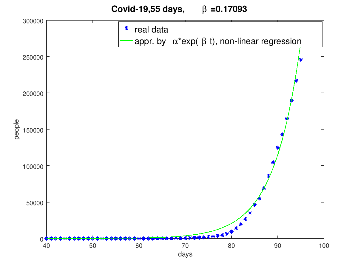
Figure 1: USA course from February 10th 2020 to April 4th 2020

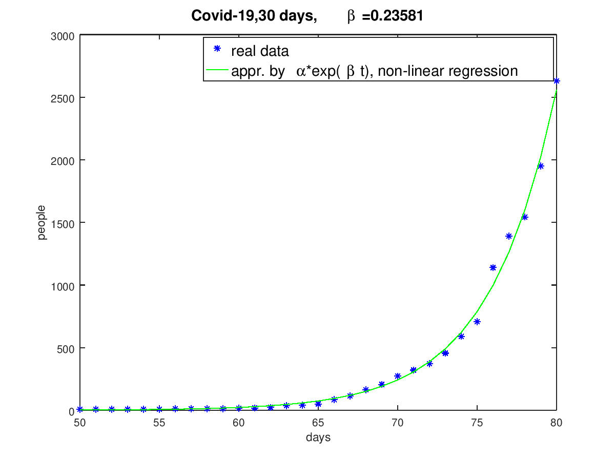
Figure 2: UK course from February 20th 2020 to March 20th 2020

It must be said that evaluated $\beta$-values are related to the stated period. For the iterative Gauss-Newton method we guessed the respective periods for every country by a visual inspection of the graphs of the infected people over days.

Especially in medicine, psychology and other life sciences the logarithm behavior of data was readily considered.

Instead of the above table of values the following logarithmic one was used.

day	log(number of infected people)
$t_{1}$	$\log I_{1}$
$t_{2}$	$\log I_{2}$
⋮	⋮
$t_{k}$	$\log I_{k}$

The logarithm of (4) leads to

$$\log I(t)=\log I_{0}+\beta t$$

and based on the logarithmic table the functional

$$L(I_{0},\beta)=\sum_{j=1}^{k}[\log I_{0}+\beta t_{j}-\log I_{j}]^{2}\;,$$

is to minimize. The solution of this linear optimization problem is trivial and it is available in most of computer algebra systems as a ”block box” of the logarithmic-linear regression.

The following figures show the results for the same periods as above for the USA and the UK.

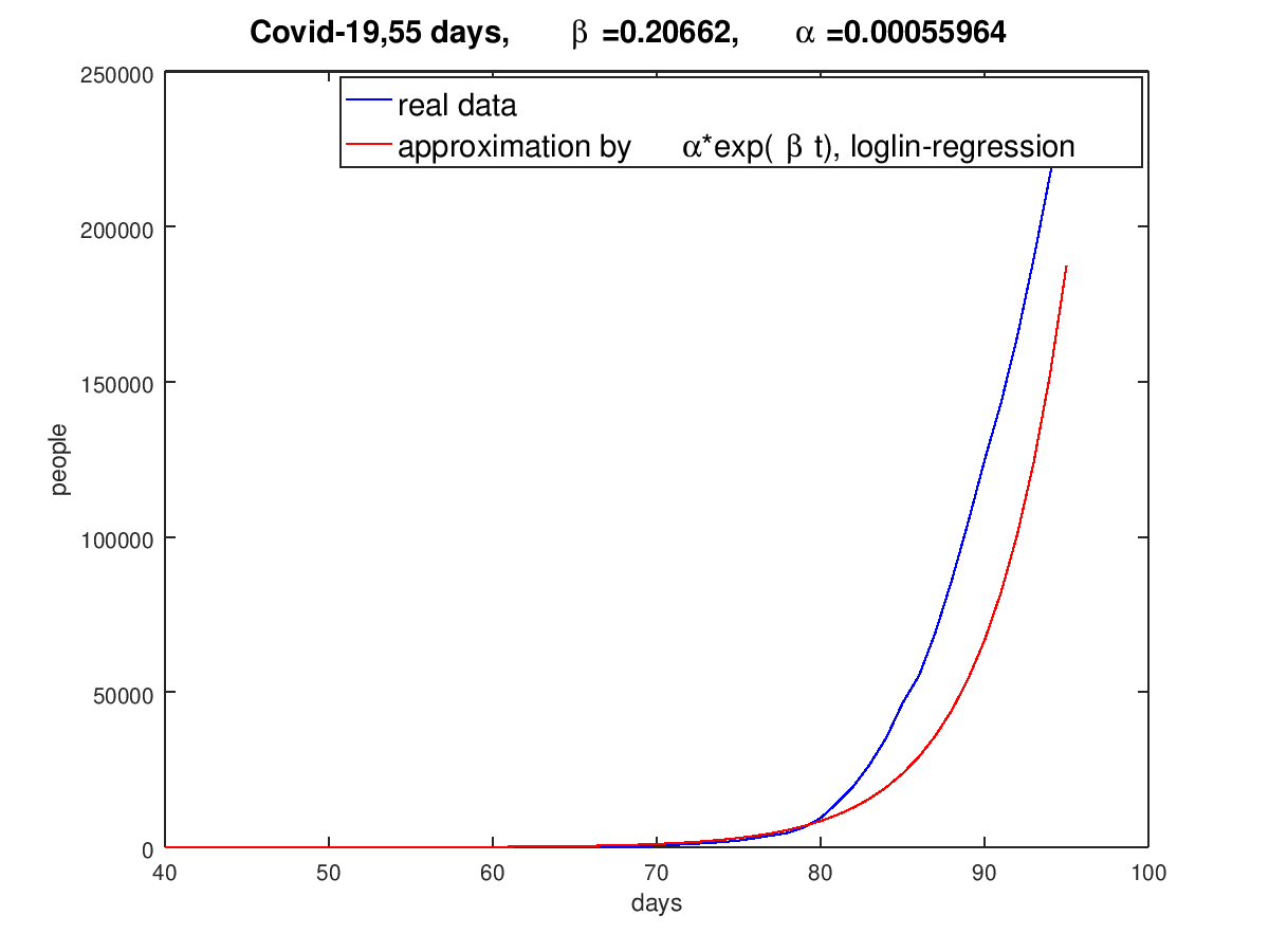
Figure 3: log-lin-result of the USA (February 10th 2020 to April 4th 2020)

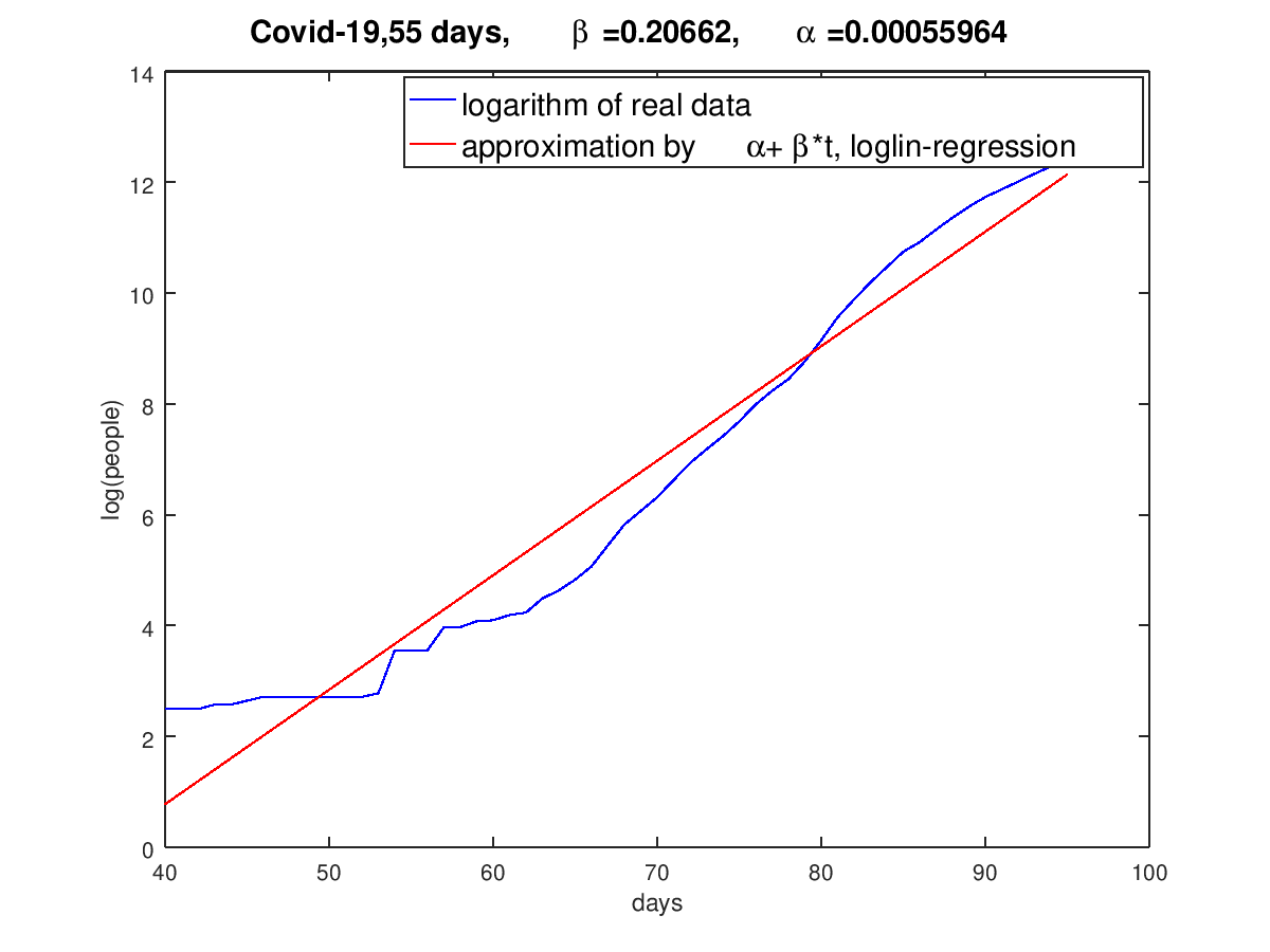
Figure 4: Logarithm of the USA result (February 10th 2020 to April 4th 2020)

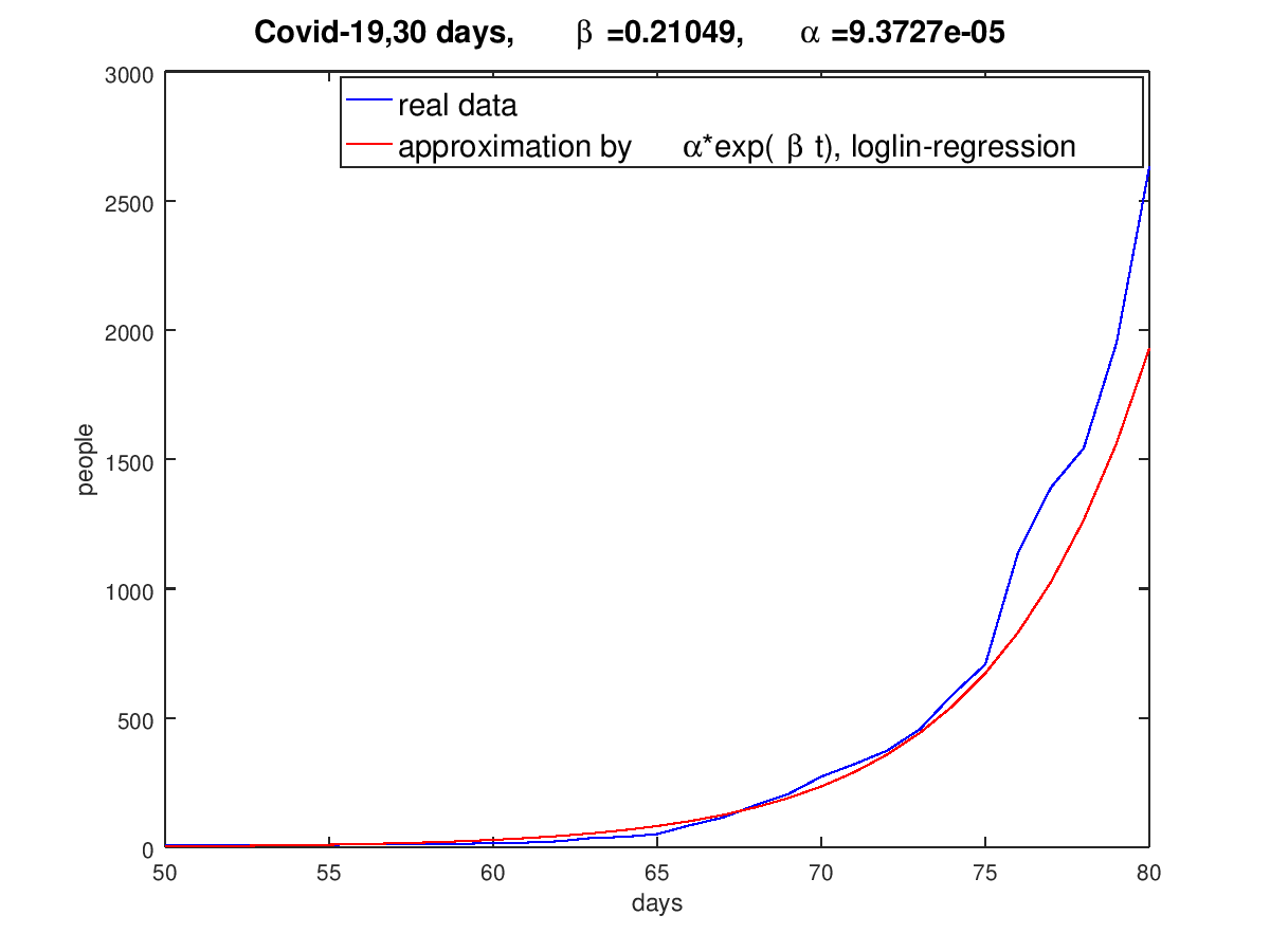
Figure 5: log-lin-result of the UK (February 20th 2020 to March 20th 2020)

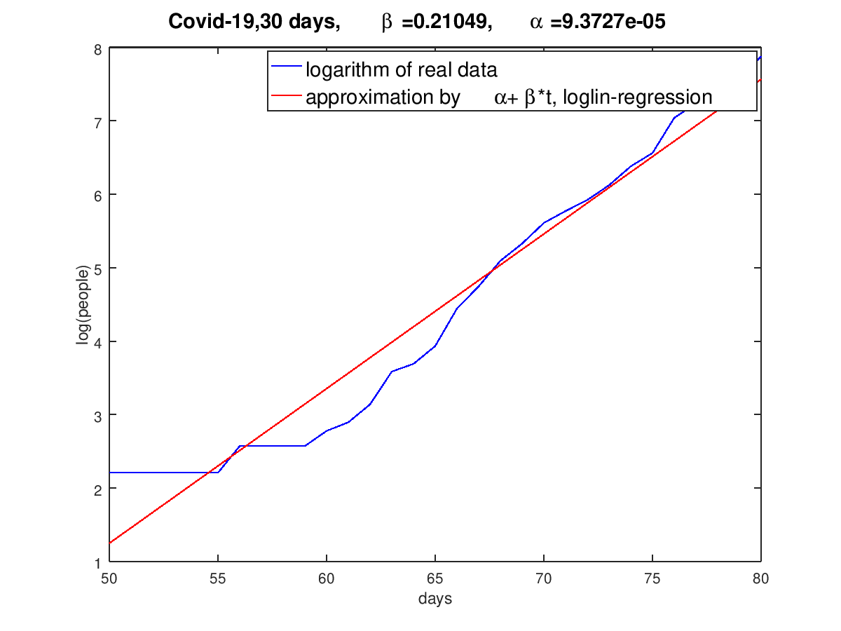
Figure 6: Logarithm of the UK result (February 20th 2020 to March 20th 2020)

Figures 4-6 show that the logarithmic-linear regression implies poor results. Thus, the non-linear optimization problem (5) is to choose as the favored method for the estimation of $I_{0}$ and $\beta$.

We found some notes on the parameters of Italy in the literature, for example $\beta=0.25$, and we are afraid that this is a result of the logarithmic-linear regression. Our result for Italy is pictured in fig. 8 and fig. 8.

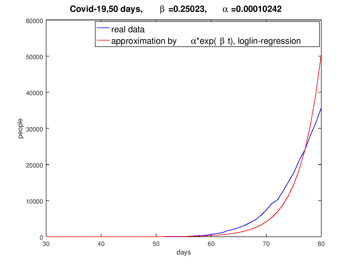
Figure 7: log-lin-result of Italy (January 31st 2020 to March 20th 2020)

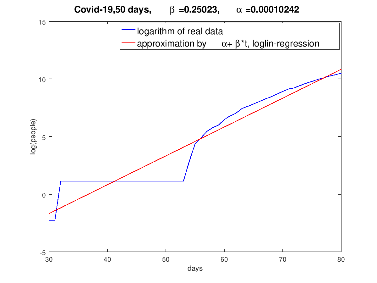
Figure 8: Logarithm of the Italian result (January 31st 2020 to March 20th 2020)

3 Some numerical computations for the USA and the UK

With the choice of $\beta$-value $0,171$ (see fig. 2) which was evaluated on the basis of the real data of ECDC and $\gamma=0,07$ one gets the course of the pandemic dynamics pictured in fig. 9.. $R_{0}$ is the basis reproduction number of persons, infected by the transmission of a pathogen from one infected person during the infectious time ($R_{0}=\beta/\gamma$) in the following figures.

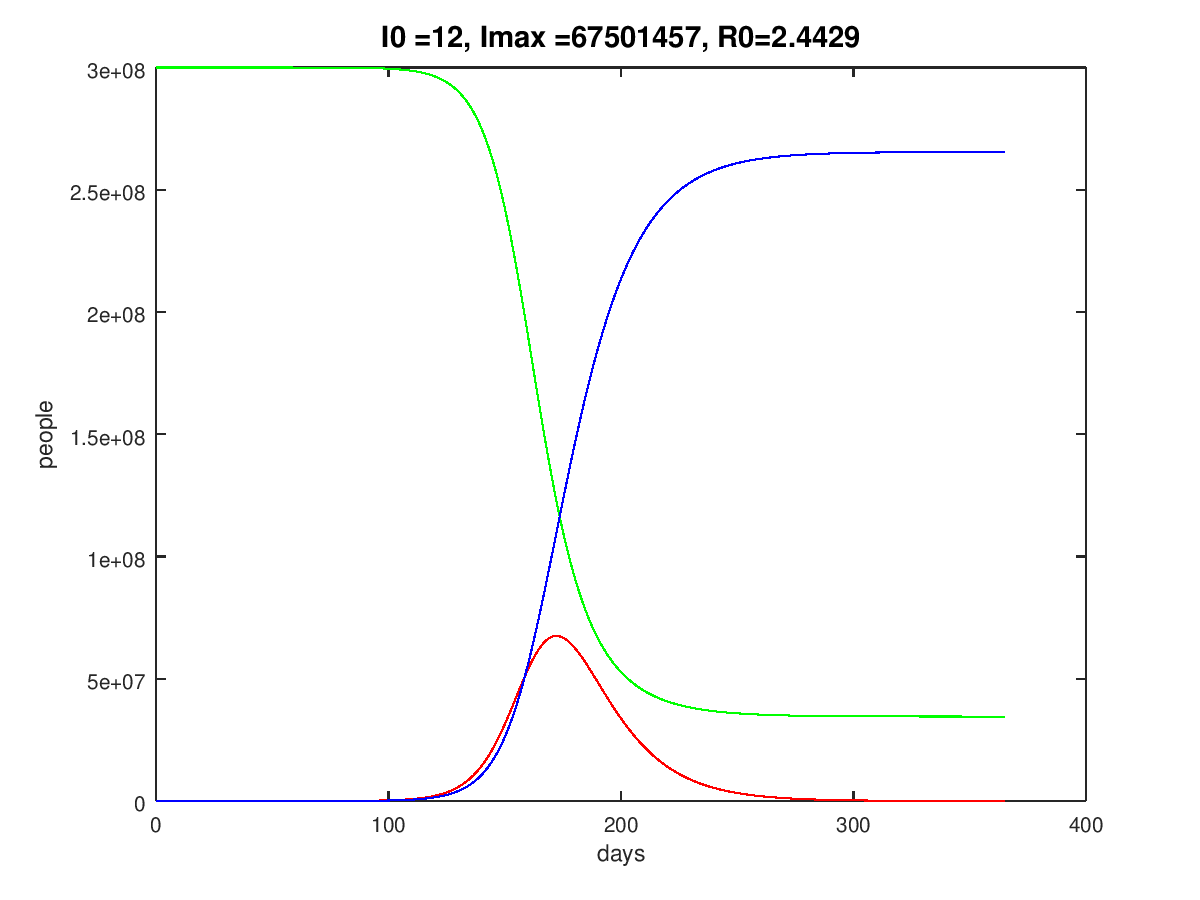
Figure 9: USA course of one year, starting February 10th 2020, $S$-green, $I$-red, $R$-blue

Neither data from ECDC nor the data from the German Robert-Koch-Institut and the data from the Johns Hopkins University are correct, for we have to reasonably assume that there are a number of unknown cases. It is guessed that the data covers only 15% of the real cases. Considering this we get a slightly changed results and in the subsequent computations we will include estimated number of unknown cases to the initial values of $I$.

For the UK we use the $\beta$-value $0,235$ (see fig. 2) and $\gamma=0,07$ we get the course pictured in fig. 10. $N$ was set to $60$ millions.

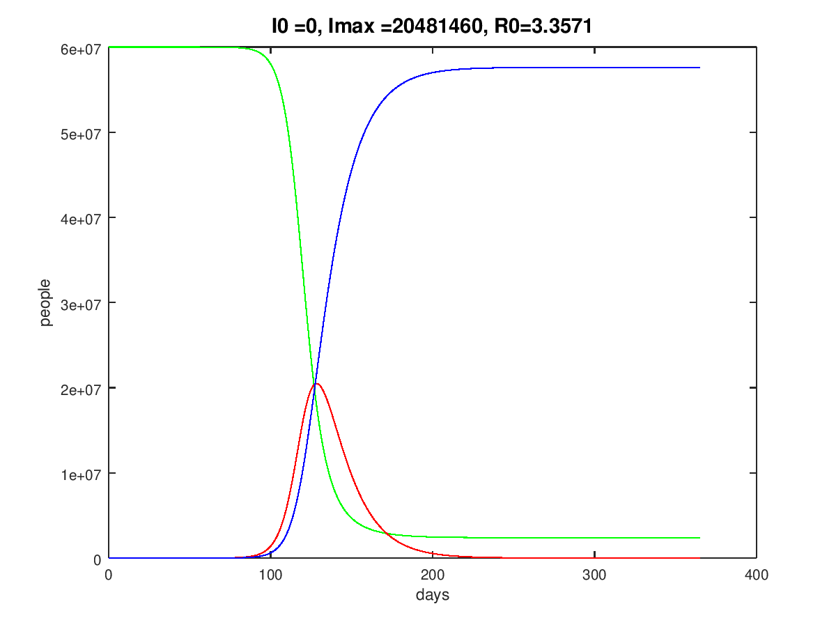
Figure 10: UK course of one year, starting February 20th 2020, $S$-green, $I$-red, $R$-blue

4 Influence of a temporary lockdown and extensive social distancing

In all countries concerned by the Corona pandemic a lockdown of the social life is discussed. In Germany the lockdown started at March 16th 2020. The effects of social distancing to decrease the infection rate can be modeled by a modification of the SIR model. The original ODE system (1)-(3) was modified to

$$\frac{dS}{dt} = -\kappa\beta\frac{S}{N}I$$ (6)

$$\frac{dI}{dt} = \kappa\beta\frac{S}{N}I-\gamma I$$ (7)

$$\frac{dR}{dt} = \gamma I\;.$$ (8)

$\kappa$ is a function with values in $[0,1]$. For example

$$\kappa(t)=\left\{\begin{array}[]{ll}0,5&\mbox{for }t_{0}\leq t\leq t_{1}\\ 1&\mbox{for }t>t_{1},\;t<t_{0}\end{array}\right.$$

means for example a reduction of the infection rate of 50% in the period $[t_{0},t_{1}]$ ($\Delta_{t}=t_{1}-t_{0}$ is the duration of the temporary lockdown in days). A good choice of $t_{0}$ and $t_{k}$ is going to be complicated.

If we respect the chosen starting day of the USA lockdown, March 31st 2020 (this conforms the 50th day of the concerned year), and we work with

$$\kappa(t)=\left\{\begin{array}[]{ll}0,2&\mbox{for }46\leq t\leq 76\\ 1&\mbox{for }t>76,\;t<46\end{array}\right.$$

we got the result pictured in fig. 11.

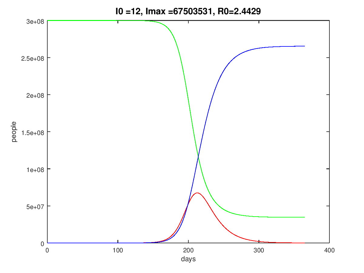
Figure 11: USA course of one year, starting February 10th 2020, $S$-green, $I$-red, $R$-blue, 30 days lockdown, starting time March 20th 2020

The numerical tests showed that a very early start of the lockdown resulting in a reduction of the infection rate $\beta$ results in the typical Gaussian curve to be delayed by $I$; however, the amplitude (maximum value of $I$) doesn’t really change.

One knows that development of the infected people looks like a Gaussian curve. The interesting points in time are those where the acceleration of the numbers of infected people increases or decreases, respectively.

These are the points in time where the curve of $I$ was changing from a convex to a concave behavior or vice versa. The convexity or concavity can be controlled by the second derivative of $I(t)$.

Let us consider equation (2). By differentiation of (2) and the use of (1) we get

$$\frac{d^{2}I}{dt^{2}} = \frac{\beta}{N}\frac{dS}{dt}I+\frac{\beta}{N}S\frac{dI}{dt}-\gamma\frac{dI}{dt}$$

$$= -\frac{\beta}{N}^{2}SI^{2}+(\frac{\beta S}{N}-\gamma)(\frac{\beta S}{N}-\gamma)I$$

$$= [(\frac{\beta S}{N}-\gamma)^{2}-(\frac{\beta}{N})^{2}SI]I\;.$$

With that the $I$-curve will change from convex to concave if the relation

$$(\frac{\beta S}{N}-\gamma)^{2}-(\frac{\beta}{N})^{2}SI<0\Longleftrightarrow I>\frac{(\frac{\beta S}{N}-\gamma)^{2}N^{2}}{\beta^{2}S}$$ (9)

is valid. For the switching time follows

$$t_{0}=\min_{t}\{t>0,\,I(t)>(\frac{\beta S(t)}{N}-\gamma)^{2}N^{2})/(\beta^{2}S(t))\}\;.$$ (10)

A lockdown starting at $t_{0}$ (assigning $\beta^{*}=\kappa\beta$,  $\kappa\in[0,1[$) up to a point in time $t_{1}=t_{0}+\Delta_{t}$, with $\Delta_{t}$ as the duration of the lockdown in days, will be denoted as a dynamical lockdown (for $t>t_{1}$ $\beta^{*}$ was reset to the original value $\beta$).

$t_{0}$ means the point in time up to which the growth rate increases and from which on it decreases. Fig. 12 shows the result of such a computation of a dynamical lockdown. We got $t_{0}=155$ ($\kappa=0,2$)- The result is significant. In fig. 14 a typical behavior of $\frac{d^{2}I}{dt^{2}}$ is plotted.

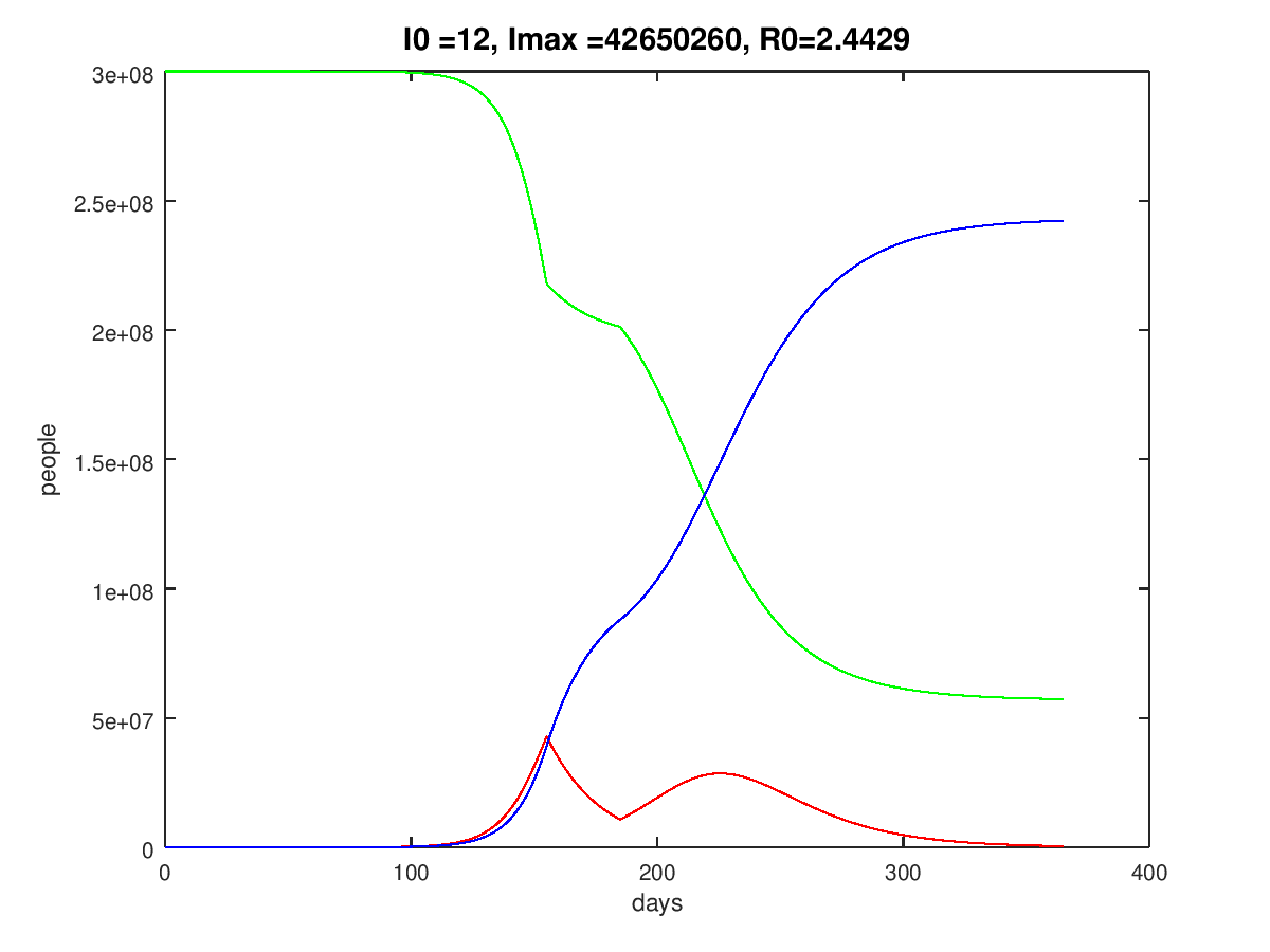
Figure 12: USA course of one year, starting February 20th 2020, dynamical lockdown, $S$-green, $I$-red, $R$-blue

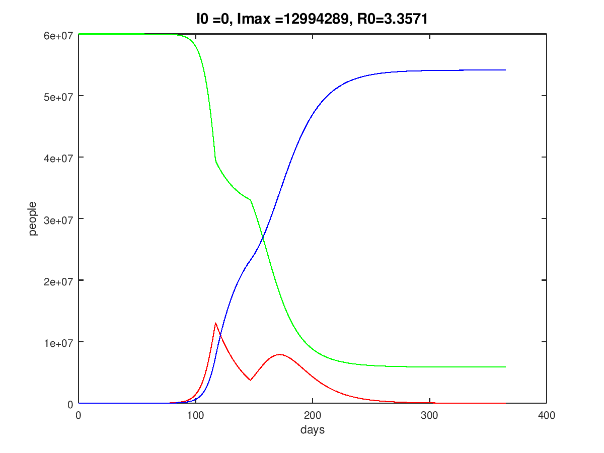
Figure 13: UK course of one year, starting February 20th 2020, dynamical lockdown, $S$-green, $I$-red, $R$-blue

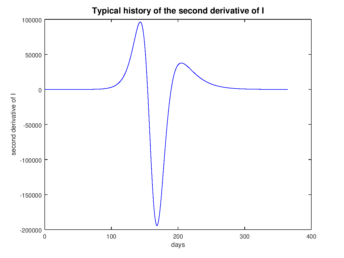
Figure 14: History of the second derivative of $I$

The result of a dynamical 30 days lockdown for the UK is shown in fig. 13, where we found $t_{0}=117$ ($\kappa=0,2$).

Data from China and South Korea suggests that the group of infected people with an age of 70 or more is of magnitude 10%. This group has a significant higher mortality rate than the rest of the infected people. Thus we can presume that $\alpha$=10% of $I$ must be especially sheltered and possibly medicated very intensively as a high-risk group.

Fig. 15 shows the USA time history of the above defined high-risk group with a dynamical lockdown with $\kappa=0,2$ compared to regime without social distancing. The maximum number of infected people decreases from approximately 6,7 millions of people to 4,2 millions in the case of the lockdown (30 days lockdown).

This result proves the usefulness of a lockdown or a strict social distancing during an epidemic disease. We observe a flattening of the infection curve as requested by politicians and health professionals. With a strict social distancing for a limited time one can save time to find vaccines and time to improve the possibilities to help high-risk people in hospitals.

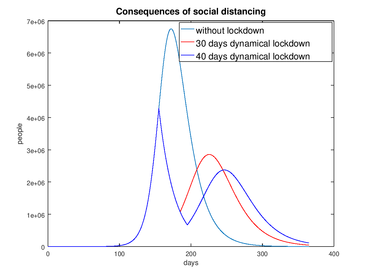
Figure 15: USA history of the infected people of high-risk groups depending on a dynamical lockdown

To see the influence of a social distancing we look at the UK situation without a lockdown and a dynamical lockdown of 30 days with fig. 16 ($\kappa=0,2$) for the 10% high-risk people.

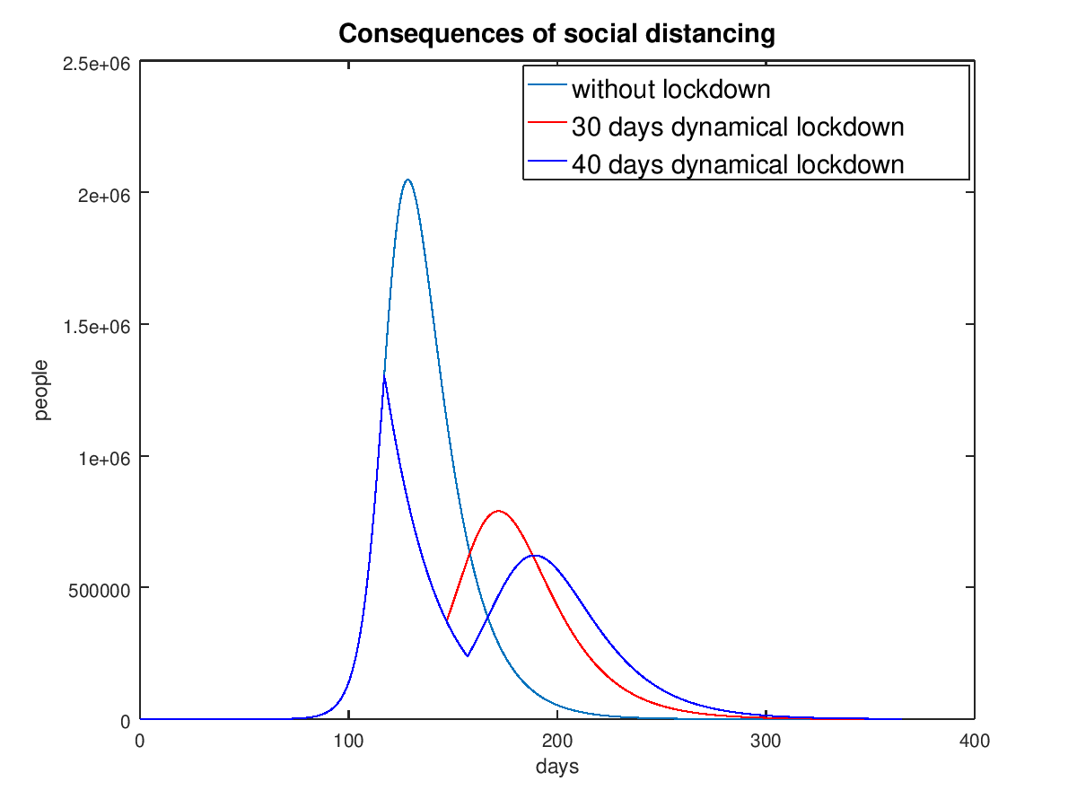
Figure 16: UK history of the infected people of high-risk groups depending on a dynamical lockdown

The computations with the SIR model show, that the social distancing with a lockdown will only be successful with a start behind the time greater or equal to $t_{0}$, found by the evaluation of the second derivative of $I$ (formula (10)). If the lockdown is started at a time less then $t_{0}$ the effect of such a social distancing is not significant.

5 Closing remarks

If we write (2) or (7) resp. in the form

$$\frac{dI}{dt}=(\kappa\beta\frac{S}{N}-\gamma)I$$

we realize that the number of infected people decreases if

$$\kappa\beta\frac{S}{N}-\gamma<0\Longleftrightarrow S<N\frac{\gamma}{\kappa\beta}$$ (11)

is complied. The relation (11) shows that there are two possibilities for the rise of infected people to be inverted and the medical burden to be reduced.

• The reduction of the stock of the species $S$. This can be obtained by immunization or vaccination. Another possibility is the isolation of high-risk people (70 years and older). Positive tests for antibodies reduce the stock of susceptible persons.

• A second possibility is the reduction of the infection rate $\kappa\beta$. This can be achieved by strict lockdowns, social distancing at appropriate times, or rigid sanitarian moves.

With respect to point a) it is important to note, that a lot of possible positive precautions by physicians and politicians can not be cover by mathematical models like the SIR one. Also the infected people are not distributed in the same way at all locations of a country. It is also possible and necessary to concentrate the modeling to hot spots like New York in the USA, Madrid in Spain or Bavaria in Germany to get a higher resolution of the pandemic behavior.

The results are pessimistic in total with respect to a successful fight against the COVID-19-virus. Hopefully the reality is a bit more merciful than the mathematical model. But we rather err on the pessimistic side and be surprised by more benign developments.

Note again that the parameters $\beta$ and $\kappa$ are guessed very roughly. Also, the percentage $\alpha$ of the group of high-risk people is possibly overestimated. Depending on the capabilities and performance of the health system of the respective countries, those parameters may look different. The interpretation of $\kappa$ as a random variable is thinkable, too.

At the end all precautions (for example social distancing, isolation of high-risk people) lead to a prolongation of the pandemic period with respect to the awaited and necessary herd immunity. But the decrease of the peak of the curve of infected people generates time for the improvement of the health systems and heights the possibilities to save life.

References

- [1] W.O. Kermack and A.G. McKendrick, A contribution to the mathematical theory of epidemics. Proc. R. Soc. London A 115(1927)700.
- [2] Bulletins of the European Centre for Disease Prevention and Control (https://www.ecdc.europa.eu/en/geographical-distribution-2019-ncov-cases) 2020.
- [3] Bulletins of the John Hopkins University of world-wide Corona data (https://www.jhu.edu) 2020.
- [4] G. Bärwolff, Numerics for engineers, physicists and computer scientists (3rd ed., in German). Springer-Spektrum 2020.
- [5] G. Bärwolff, A Contribution to the Mathematical Modeling of the Corona/COVID-19 Pandemic. medRxiv.preprint 2020, doi: https://doi.org/10.1101/2020.04.01.20050229.
- [6] Toshihisa Tomie, Understandig the present status and forcasting of COVID-19 in Wuhan. medRxiv.preprint 2020.