The Estimation of the Effective Reproductive Number from Disease Outbreak Data

Abstract

We consider a single outbreak susceptible-infected-recovered (SIR) model and corresponding estimation procedures for the effective reproductive number $\mathcal{R}(t)$. We discuss the estimation of the underlying SIR parameters with a generalized least squares (GLS) estimation technique. We do this in the context of appropriate statistical models for the measurement process. We use asymptotic statistical theories to derive the mean and variance of the limiting (Gaussian) sampling distribution and to perform post statistical analysis of the inverse problems. We illustrate the ideas and pitfalls (e.g., large condition numbers on the corresponding Fisher information matrix) with both synthetic and influenza incidence data sets.

Keywords

Effective reproductive number, basic reproduction ratio, reproduction number, $\mathcal{R}$, $\mathcal{R}(t)$, $\mathcal{R}_{0}$, parameter estimation, ordinary least squares, generalized least squares.

1 Introduction

The transmissibility of an infection can be quantified by its basic reproductive number, $\mathcal{R}_{0}$, defined as the mean number of secondary infections seeded by a typical infective into a completely susceptible (naive) host population [1, 14, 20]. For many simple epidemic processes, this parameter determines a threshold: whenever $\mathcal{R}_{0}>1$, a typical infective gives rise to more than one secondary infection, leading to an epidemic. In contrast, when $\mathcal{R}_{0}<1$, infectives typically give rise to less than one secondary infection and the prevalence of infection cannot increase.

Due to the natural history of some infections, transmissibility is better quantified by the effective—rather than the basic—reproductive number. For instance, exposure to influenza in previous years confers some cross-immunity [11, 17, 25]; the strength of this protection depends on the antigenic similarity between the current year’s strain of influenza and earlier ones. Consequently, the population is non-naive and so it is more appropriate to consider the effective reproductive number, $\mathcal{R}(t)$, a time-dependent quantity that accounts for the population’s reduced susceptibility.

Our goal is to develop a methodology for the estimation of $\mathcal{R}(t)$ that also provides a measure of the uncertainty in the estimates. We apply the proposed methodology in the context of annual influenza outbreaks, focusing on data for influenza A (H3N2) viruses, which were, with the exception of the influenza seasons 2000-1 and 2002-3, the dominant flu subtype in the US over the period from 1997 to 2005 [9, 29].

The estimation of reproductive numbers is typically an indirect process because some of the parameters on which these numbers depend are difficult, if not impossible, to quantify directly. A commonly used indirect approach involves fitting a model to some epidemiological data, providing estimates of the required parameters.

In this study we estimate the effective reproductive number by fitting a deterministic epidemiological model employing either an Ordinary Least-Squares (OLS) or a Generalized Least-Squares (GLS) estimation scheme to obtain estimates of model parameters. Statistical asymptotic theory [13, 27] and sensitivity analysis [12, 26] are then applied to give approximate sampling distributions for the estimated parameters. Uncertainty in the estimates of $\mathcal{R}(t)$ is then quantified by drawing parameters from these sampling distributions, simulating the corresponding deterministic model and then calculating effective reproductive numbers. In this way, the sampling distribution of the effective reproductive number is constructed at any desired time point.

The statistical methodology provides a framework within which the adequacy of the parameter estimates can be formally assessed for a given data set. We shall present instances in which the fitted model appears to provide an adequate fit to a given data set but where the statistics reveal that the parameter estimates have very high levels of uncertainty. We also discuss situations in which the fitted model appears, at least visually, to provide an adequate fit and where the statistics suggest that the uncertainty in the parameters is not so large but that, in reality, a poor fit has been achieved. We discuss the use of residuals plots as a diagnostic for this outcome, which highlights the problems that arise when the assumptions of the statistical model underlying the estimation framework are violated.

This manuscript is organized as follows: In Section 2 the data sets are introduced. A single-outbreak deterministic model is introduced in Section 3. Section 4 introduces the least squares estimation methodology used to estimate values for the parameters and quantify the uncertainty in these estimates. Our methodology for obtaining estimates of $\mathcal{R}(t)$ and its uncertainty is also described. Use of these schemes is illustrated in Section 5, in which they are applied to synthetic data sets. Section 6 applies the estimation machinery to the influenza incidence data sets. We conclude with a discussion of the methodologies and their application to the data sets.

2 Longitudinal Incidence Data

Table 1: Number of tested specimens and influenza isolates during several annual outbreaks in the US [9].

Season	Total number of	Number of A(H1N1) &	Number of	Number of
	tested specimens	A(H1N2) isolates	A(H3N2) isolates	B isolates
1997-1998	99,072	6	3,241	102
1998-1999	102,105	30	2,607	3,370
1999-2000	92,403	132	3,640	77
2000-2001	88,598	2,061	66	4,625
2001-2002	100,815	87	4,420	1,965
2002-2003	97,649	2,228	942	4,768
2003-2004	130,577	2	7,189	249
2004-2005	157,759	18	5,801	5,799
Mean	108,622	571	3,488	2,619

Figure 1: Influenza isolates reported by the CDC in the US during the 1999-2000 season [9]. The number of H3N2 cases (isolates) is displayed as a function of time. Time is measured as the number of weeks since the start of the year’s flu season. For the 1999-2000 flu season, week number one corresponds to the fortieth week of the year, falling in October.

Influenza is one of the most significant infectious diseases of humans, as witnessed by the 1918 “Spanish Flu” pandemic, during which 20 to 40 percent of the worldwide population became infected. At least 50 million deaths resulted, with 675,000 of these occurring in the US [30]. The impact of flu is still significant during inter-pandemic periods: the Centers for Disease Control and Prevention (CDC) estimate that between 5 and 20 percent of the US population becomes infected annually [9]. These annual flu outbreaks lead to an average of 200,000 hospitalizations (mostly involving young children and the elderly) and mortality that ranges between about 900 and 13,000 deaths per year [29].

The Influenza Division of the CDC reports weekly information on influenza activity in the US from calendar week 40 in October through week 20 in May [9], the period referred to as the influenza season. Because the influenza virus exhibits a high degree of genetic variability, data is not only collected on the number of cases but also on the types of influenza viruses that are circulating. A sample of viruses isolated from patients undergoes antigenic characterization, with the type, subtype and, in some instances, the strain of the virus being reported [9].

The CDC acknowledges that, while these reports may help in mapping influenza activity (whether or not it is increasing or decreasing) throughout the US, they do not provide enough information to calculate how many people became ill with influenza during a given season. The CDC’s caution likely reflects the uncertainty associated with the sampling process that gives rise to the tested isolates, in particular that this process is not sufficiently standardized across space and time. We return to discuss this point later in this paper.

Despite the cautionary remarks by the CDC we use these isolate reports as illustrative data sets to which we can apply our proposed estimation methodologies. Interpretation of the results, however, should be mindful of the issues associated with the data. The total number of tested specimens and isolates through various seasons are summarized in Table 1. It is observed that H3N2 viruses predominated in most seasons with the exception of 2000-1 and 2002-3. Consequently, we focus our attention on the H3N2 subtype. Figure 1 depicts the number of H3N2 isolates reported over the 1999-2000 influenza season.

3 Deterministic Single-Outbreak SIR Model

The model that we use is the standard Susceptible-Infective-Recovered (SIR) model (see, for example, [1, 6]). The state variables $S(t)$, $I(t)$, and $R(t)$ denote the number of people who are susceptible, infective, and recovered, respectively, at time $t$. It is assumed that newly infected individuals immediately become infectious and that recovered individuals acquire permanent immunity. The influenza season, lasting nearly 32 weeks [9], is short compared to the average lifespan, so we ignore demographic processes (births and deaths) as well as disease-induced fatalities and assume that the total population size remains constant. The model is given by the following set of nonlinear differential equations

$$\frac{dS}{dt} = -\beta S\frac{I}{N}$$ (1)

$$\frac{dI}{dt} = \beta S\frac{I}{N}-\gamma I$$ (2)

$$\frac{dR}{dt} = \gamma I.$$ (3)

Here, $\beta$ is the transmission parameter and $\gamma$ is the (per-capita) rate of recovery, the reciprocal of which gives the average duration of infection. Notice that one of the differential equations is redundant because the three compartments sum to the constant population size: $S(t)+I(t)+R(t)=N$. We choose to track $S(t)$ and $I(t)$. The initial conditions of these state variables are denoted by $S(t_{0})=S_{0}$ and $I(t_{0})=I_{0}$.

The equation for the infective population (2) can be rewritten as

$$\frac{dI}{dt}=\gamma(\mathcal{R}(t)-1)I,$$ (4)

where $\mathcal{R}(t)=\frac{S(t)}{N}\mathcal{R}_{0}$ and $\mathcal{R}_{0}=\beta/\gamma$. $\mathcal{R}(t)$ is known as the effective reproductive number, while $\mathcal{R}_{0}$ is known as the basic reproductive number. We have that $\mathcal{R}(t)\leq\mathcal{R}_{0}$, with the upper bound—the basic reproductive number—only being achieved when the entire population is susceptible.

We note that $\mathcal{R}(t)$ is the product of the per-infective rate at which new infections arise and the average duration of infection, and so the effective reproductive number gives the average number of secondary infections caused by a single infective, at a given susceptible fraction. The prevalence of infection increases or decreases according to whether $\mathcal{R}(t)$ is greater than or less than one, respectively. Because there is no replenishment of the susceptible pool in this SIR model, $\mathcal{R}(t)$ decreases over the course of an outbreak as susceptible individuals become infected.

4 Estimation Schemes

In order to calculate $\mathcal{R}(t)$, it is necessary to know the two epidemiological parameters $\beta$ and $\gamma$, as well as the number of susceptibles, $S(t)$, and the population size, $N$. As mentioned before, difficulties in the direct estimation of $\beta$—whose value reflects the rate at which contacts occur in the population and the probability of transmission occurring when a susceptible and infective meet—and direct estimation of $S(t)$ preclude direct estimation of $\mathcal{R}(t)$. As a result, we adopt an indirect approach, which proceeds by first finding the parameter set for which the model has the best agreement with the data and then calculating $\mathcal{R}(t)$ by using these parameters and the model-predicted time course of $S(t)$. Simulation of the model also requires knowledge of the initial values, $S_{0}$ and $I_{0}$, which must also be estimated.

Although the model is framed in terms of the prevalence of infection $I(t)$, the time-series data provides information on the weekly incidence of infection, which, in terms of the model, is given by the integral of the rate at which new infections arise over the week: $\int\beta S(t)I(t)/N\,dt$. We notice that the parameters $\beta$ and $N$ only appear (both in the model and in the expression for incidence) as the ratio $\beta/N$, precluding their separate estimation. Consequently we need only estimate the value of this ratio, which we call $\tilde{\beta}=\beta/N$.

We employ inverse problem methodology to obtain estimates of the vector $\theta=(S_{0},I_{0},\tilde{\beta},\gamma)\in\mathbb{R}^{p}=\mathbb{R}^{4}$ by minimizing the difference between the model predictions and the observed data, according to two related but distinct least squares criteria, ordinary least squares (OLS) and generalized least squares (GLS). In what follows, we refer to $\theta$ as the parameter vector, or simply the parameter, in the inverse problem, even though some of its components are initial conditions, rather than parameters, of the underlying dynamic model.

4.1 Ordinary Least Squares (OLS) Estimation

The least squares estimation methodology is based on the mathematical model as well as a statistical model for the observation process (referred to as the case counting process). It is assumed that our known model, together with a particular choice of parameters— the “true” parameter vector, written as $\theta_{0}$—exactly describes the epidemic process, but that the $n$ observations, $Y_{j}$, are affected by random deviations (e.g., measurement errors) from this underlying process. More precisely, it is assumed that

$$\begin{array}[]{lccr}Y_{j}=z(t_{j};\theta_{0})+\epsilon_{j}&&&\mbox{ for $j=1,\dots,n$}\end{array}$$ (5)

where $z(t_{j};\theta_{0})$ denotes the weekly incidence given by the model under the true parameter, $\theta_{0}$, and is defined by the following integral:

$$z(t_{j};\theta_{0})=\int_{t_{j-1}}^{t_{j}}\tilde{\beta}S(t;\theta_{0})I(t;\theta_{0})\,dt.$$ (6)

Here, $t_{0}$ denotes the time at which the epidemic observation process started and the weekly observation time points are written as $t_{1}<\dots<t_{n}$.

The errors, $\epsilon_{j}$, are assumed to be independent and identically distributed (i.i.d.) random variables with zero mean ($E[\epsilon_{j}]=0$), representing measurement error as well as other phenomena that cause the observations to deviate from the model predictions $z(t_{j};\theta_{0})$. The i.i.d. assumption means that the errors are uncorrelated across time and that each has identical variance, which we write as $var(\epsilon_{j})=\sigma_{0}^{2}$. It is assumed that $\sigma_{0}^{2}$ is finite. We make no further assumptions about the distribution of the errors: in particular, we do not assume that they are normally distributed. It is immediately clear that we have $E[Y_{j}]=z(t_{j};\theta_{0})$ and $var(Y_{j})=\sigma_{0}^{2}$: in particular, this variance is longitudinally constant (i.e, across the time points).

For a given set of observations $Y=(Y_{1},\dots,Y_{n})$, we define the estimator $\theta_{OLS}$ as follows:

$$\theta_{OLS}(Y)=\theta_{OLS}^{n}(Y)=\mbox{arg}\min_{\theta\in\Theta}\sum_{j=1}^{n}\left[Y_{j}-z(t_{j};\theta)\right]^{2}.$$ (7)

Here $\Theta$ represents the feasible region for the parameter values. (We discuss this region in more detail later.) This estimator is a random variable (note that $\epsilon_{j}=Y_{j}-z(t_{j};\theta_{0})$ is a random variable) that involves minimizing the distance between the data and the model prediction. We note that all of the observations are treated as having equal importance in the OLS formulation.

If $\{y_{j}\}_{j=1}^{n}$ is a realization of the case counting (random) process $\{Y_{j}\}_{j=1}^{n}$, we define the cost function by

$$J(\theta)=\sum_{j=1}^{n}\left[y_{j}-z(t_{j};\theta)\right]^{2}$$ (8)

and observe that the solution of

$$\hat{\theta}_{OLS}=\hat{\theta}_{OLS}^{n}=\mbox{arg}\min_{\theta\in\Theta}J(\theta)$$ (9)

provides a realization of the random variable $\theta_{OLS}$.

The optimization problem in Equation (9) can, in principle, be solved by a wide variety of algorithms. The results discussed in this paper were obtained by using a direct search method, the Nelder-Mead simplex algorithm, as discussed by [22], employing the implementation provided by the MATLAB (The Mathworks, Inc.) routine fminsearch.

Because $var(\epsilon_{j})=E(\epsilon^{2}_{j})=\sigma_{0}^{2}$, the true variance satisfies

$$\sigma_{0}^{2}=\frac{1}{n}E\left[\sum_{j=1}^{n}\left[Y_{j}-z(t_{j};\theta_{0})\right]^{2}\right].$$ (10)

Because we do not know $\theta_{0}$, we base our estimate of the error variance on an equation of this form, but instead of using $\theta_{0}$ we use the estimated parameter vector, $\hat{\theta}_{OLS}$. The right side of Equation (10) is then equal to $J(\hat{\theta}_{OLS})/n$. This estimate, however, is biased and so instead the following bias-adjusted estimate is used

$$\hat{\sigma}^{2}_{OLS}=\frac{1}{n-4}J(\hat{\theta}_{OLS}).$$ (11)

Here the $n-4$ arises because $p=4$ parameters have been estimated from the data.

Even though the distribution of the errors is not specified, asymptotic theory can be used to describe the distribution of the random variable $\theta_{OLS}$ [3, 27]. Provided that a number of regularity conditions as well as sampling conditions are met (see [27] for details), it can be shown that, asymptotically (i.e., as $n\rightarrow\infty$), $\theta_{OLS}$ is distributed according to the following multivariate normal distribution:

$$\theta_{OLS}=\theta^{n}_{OLS}\sim\mathcal{N}_{4}\left(\theta_{0},\Sigma_{0}^{n}\right),$$ (12)

where $\Sigma_{0}^{n}=n^{-1}\sigma^{2}_{0}\Omega_{0}^{-1}$ and

$$\Omega_{0}=\lim_{n\rightarrow\infty}\frac{1}{n}\chi(\theta_{0},n)^{T}\chi(\theta_{0},n).$$ (13)

We remark that the theory requires that this limit exists and that the matrix $\Omega_{0}$ be non-singular. The matrix $\Sigma_{0}^{n}$ is the $4\times 4$ covariance matrix, whose entries equal $cov\left((\theta_{OLS})_{i},(\theta_{OLS})_{j}\right)$, and the $n\times 4$ matrix $\chi(\theta_{0},n)$ is the sensitivity matrix of the system, as defined and discussed below.

In general, $\theta_{0}$, $\sigma_{0}^{2}$, and $\Sigma_{0}^{n}$ are unknown, so these quantities are approximated by the estimates $\hat{\theta}_{OLS}$ and $\hat{\sigma}^{2}_{OLS}$, and the following matrix

$$\Sigma_{0}^{n}\approx\hat{\Sigma}_{OLS}^{n}=\hat{\sigma}_{OLS}^{2}\left[\chi(\hat{\theta}_{OLS},n)^{T}\chi(\hat{\theta}_{OLS},n)\right]^{-1}.$$ (14)

Consequently, for large $n$, we have approximately that

$$\theta_{OLS}=\theta^{n}_{OLS}\sim\mathcal{N}_{4}\left(\hat{\theta}_{OLS},\hat{\sigma}_{OLS}^{2}\left[\chi(\hat{\theta}_{OLS},n)^{T}\chi(\hat{\theta}_{OLS},n)\right]^{-1}\right).$$ (15)

We obtain the standard error for the $i$-th element of $\hat{\theta}_{OLS}$ by calculating $\sqrt{\left(\hat{\Sigma}^{n}_{OLS}\right)_{ii}}$.

The $n\times 4$ matrices $\chi(\theta,n)$ that appear in the above formulae are called sensitivity matrices and are defined by

$$\chi_{ji}(\theta,n)=\frac{\partial z(t_{j};\theta)}{\partial\theta_{i}},{\rm\qquad}1\leq j\leq n,\ \ 1\leq i\leq 4.$$ (16)

The sensitivity matrix denotes the variation of the model output with respect to the parameter, and, for this model-based dynamical system, can be obtained using standard theory [2, 12, 16, 19, 21, 26].

The entries of the $j$-th row of $\chi(\theta,n)$ denote how the weekly incidence at time $t_{j}$ changes in response to changes in the parameter (i.e., in either $S_{0}$, $I_{0}$, $\tilde{\beta}$, or $\gamma$) and these can be calculated by

$$\frac{\partial z}{\partial S_{0}}(t_{j};\theta) = \tilde{\beta}\int_{t_{j-1}}^{t_{j}}\left[I(t;\theta)\frac{\partial S}{\partial S_{0}}(t;\theta)+S(t;\theta)\frac{\partial I}{\partial S_{0}}(t;\theta)\right]dt$$ (17)

$$\frac{\partial z}{\partial I_{0}}(t_{j};\theta) = \tilde{\beta}\int_{t_{j-1}}^{t_{j}}\left[I(t;\theta)\frac{\partial S}{\partial I_{0}}(t;\theta)+S(t;\theta)\frac{\partial I}{\partial I_{0}}(t;\theta)\right]dt$$ (18)

$$\frac{\partial z}{\partial\tilde{\beta}}(t_{j};\theta) = \int_{t_{j-1}}^{t_{j}}\left[S(t;\theta)I(t;\theta)+\tilde{\beta}\left(I(t;\theta)\frac{\partial S}{\partial\tilde{\beta}}(t;\theta)+S(t;\theta)\frac{\partial I}{\partial\tilde{\beta}}(t;\theta)\right)\right]dt$$ (19)

$$\frac{\partial z}{\partial\gamma}(t_{j};\theta) = \tilde{\beta}\int_{t_{j-1}}^{t_{j}}\left[I(t;\theta)\frac{\partial S}{\partial\gamma}(t;\theta)+S(t;\theta)\frac{\partial I}{\partial\gamma}(t;\theta)\right]dt.$$ (20)

We see that these expressions involve the partial derivatives of the state variables, $S(t;\theta)$ and $I(t;\theta)$, with respect to the parameters. Analytic forms of the sensitivities are not available because the state variables are the solutions of a nonlinear system; instead, they are calculated numerically.

In order to outline how these numerical sensitivities may be found, we introduce the notation $x(t;\theta)=(S(t;\theta),I(t;\theta))$ and denote by $g=(g_{1},g_{2})$ the vector function whose entries are given by the expressions on the right sides of Equations (1) and (2). Then we can write the single-outbreak SIR model in the general vector form

$$\frac{dx}{dt}(t;\theta) = g(x(t;\theta);\theta)$$ (21)

$$x(0;\theta) = (\theta_{1},\theta_{2}).$$ (22)

Because the function $g$ is differentiable (in both $t$ and $\theta$), taking the partial derivatives $\partial/\partial\theta$ of both sides of Equation (21) we obtain the differential equation

$$\frac{d}{dt}\frac{\partial x}{\partial\theta}=\frac{\partial g}{\partial x}\frac{\partial x}{\partial\theta}+\frac{\partial g}{\partial\theta}.$$ (23)

Here ${\partial g}/{\partial x}$ is a 2-by-2 matrix, ${\partial g}/{\partial\theta}$ is a 2-by-4 matrix, and ${\partial x}/{\partial\theta}$ is the 2-by-4 matrix

$$\frac{\partial x}{\partial\theta}=\left[\begin{array}[]{cccc}\frac{\partial S}{\partial S_{0}}&\frac{\partial S}{\partial I_{0}}&\frac{\partial S}{\partial\tilde{\beta}}&\frac{\partial S}{\partial\gamma}\\ \frac{\partial I}{\partial S_{0}}&\frac{\partial I}{\partial I_{0}}&\frac{\partial I}{\partial\tilde{\beta}}&\frac{\partial I}{\partial\gamma}\end{array}\right].$$ (24)

Numerical values of the sensitivities are calculated by solving (21) and (23) simultaneously. We define $\phi(t)=\frac{\partial x}{\partial\theta}(t;\theta)$, let the parameter be evaluated at the estimate, $\theta=\hat{\theta}$, and solve the following differential equations from $t=0$ to $t=t_{n}$

$$\frac{d}{dt}x(t) = g(x(t;\hat{\theta});\hat{\theta})$$ (25)

$$\frac{d}{dt}\phi(t) = \frac{\partial g}{\partial x}\phi(t)+\frac{\partial g}{\partial\theta}$$ (26)

$$x(0) = (\hat{\theta}_{1},\hat{\theta}_{2})$$ (27)

$$\phi(0) = \left[\begin{array}[]{cccc}1&0&0&0\\ 0&1&0&0\end{array}\right].$$ (30)

4.2 Generalized Least Squares (GLS) Estimation

The errors in the statistical model defined by Equation (5) were assumed to have constant variance, which may not be an appropriate assumption for all data sets. One alternative statistical model that can account for more complex error structure in the case counting process is the following

$$Y_{j}=z(t_{j};\theta_{0})\left(1+\epsilon_{j}\right).$$ (31)

As before, it is assumed the $\epsilon_{j}$ are i.i.d. random variables with $E(\epsilon_{j})=0$ and $var(\epsilon_{j})=\sigma_{0}^{2}<\infty$, but no further assumptions are made. Under these assumptions, the observation mean is again equal to the model prediction, $E[Y_{j}]=z(t_{j};\theta_{0})$, while the variance in the observations is a function of the time point, with $var(Y_{j})=\sigma_{0}^{2}z^{2}(t_{j};\theta_{0})$. In particular, this variance is non-constant and model-dependent. One situation in which this error structure may be appropriate is when observation errors scale with the size of the measurement (so-called relative noise).

Given a set of observations $Y=(Y_{1},\dots,Y_{n})$, the estimator $\theta_{GLS}=\theta_{GLS}(Y)$ is defined as the solution of the normal equations

$$\sum^{n}_{j=1}w_{j}\left[Y_{j}-z(t_{j};\theta)\right]\nabla_{\theta}z(t_{j};\theta)=0,$$ (32)

where the $w_{j}$ are a set of non-negative weights [13]. Unlike the ordinary least squares formulation, this definition assigns different levels of influence, described by the weights, to the different observations in the cost function. For the error structure described above in Equation (31), the weights are taken to be inversely proportional to the square of the predicted incidence: $w_{j}=1/[z(t_{j};\theta)]^{2}$. We shall also consider weights taken to be proportional to the reciprocal of the predicted incidence; these correspond to assuming that the variance in the observations is proportional to the value of the model (as opposed to its square).

Suppose $\{y_{j}\}_{j=1}^{n}$ is a realization of the case counting process $\{Y_{j}\}_{j=1}^{n}$ and define the function $L(\theta)$ as

$$L(\theta)=\sum_{j=1}^{n}w_{j}\left[y_{j}-z(t_{j};\theta)\right]^{2}$$ (33)

The quantity $\theta_{GLS}$ is a random variable and a realization of it, denoted by $\hat{\theta}_{GLS}$, is obtained by solving

$$\sum^{n}_{j=1}w_{j}\left[y_{j}-z(t_{j};\theta)\right]\nabla_{\theta}z(t_{j};\theta)=0,$$ (34)

In the limit as $n\rightarrow\infty$, the GLS estimator $\theta_{GLS}$ has the following asymptotic properties [3, 13]:

$$\theta_{GLS}=\theta^{n}_{GLS}\sim\mathcal{N}_{4}(\theta_{0},\Sigma_{0}^{n})$$ (35)

where

$$\Sigma^{n}_{0}\approx\sigma_{0}^{2}\left[\chi(\theta_{0},n)^{T}W(\theta_{0})\chi(\theta_{0},n)\right]^{-1}.$$ (36)

Here $W(\theta_{0})=diag(w_{1}(\theta_{0}),\dots,w_{n}(\theta_{0}))$ with $w_{j}(\theta_{0})=1/[z(t_{j};\theta_{0})]^{2}$. The sensitivity matrix $\chi(\theta_{0},n)$ is as defined in Section 4.1.

Because $\theta_{0}$ and $\sigma_{0}^{2}$ are unknown, the estimate $\hat{\theta}_{GLS}$ is used to calculate approximations of $\sigma_{0}^{2}$ and the covariance matrix $\Sigma_{0}^{n}$ by

$$\sigma_{0}^{2}\approx\hat{\sigma}_{GLS}^{2}=\frac{1}{n-4}L(\hat{\theta}_{GLS})$$ (37)

$$\Sigma_{0}^{n}\approx\hat{\Sigma}_{GLS}^{n}=\hat{\sigma}^{2}_{GLS}\left[\chi(\hat{\theta}_{GLS},n)^{T}W(\hat{\theta}_{GLS})\chi(\hat{\theta}_{GLS},n)\right]^{-1}.$$ (38)

As before, the standard errors for $\hat{\theta}_{GLS}$ can be approximated by taking the square roots of the diagonal elements of the covariance matrix $\hat{\Sigma}^{n}_{GLS}$.

The cost function used in GLS estimation involves weights whose values depend on the values of the fitted model. These values are not known before carrying out the estimation procedure and consequently GLS estimation is implemented as an iterative process. An OLS is first performed on the data, and the resulting model values provide an initial set of weights. A weighted least squares fit is then performed using these weights, obtaining updated model values and hence an updated set of weights. The weighted least squares process is repeated until some convergence criterion is satisfied, such as successive values of the estimates being deemed to be sufficiently close to each other. The process can be summarized as follows

1. Estimate $\hat{\theta}_{GLS}$ by $\hat{\theta}^{(0)}$ using the OLS Equation (9). Set $k=0$;

2. Form the weights $\hat{w}_{j}=1/[z(t_{j};\hat{\theta}^{(k)})]^{2}$;

3. Define $L(\theta)=\sum_{j=1}^{n}\hat{w}_{j}[y_{j}-z(t_{j};\theta)]^{2}$. Re-estimate $\hat{\theta}_{GLS}$ by solving

   $$\hat{\theta}^{(k+1)}=\mbox{arg}\min_{\theta\in\Theta}L(\theta)$$

   to obtain the $k+1$ estimate $\hat{\theta}^{(k+1)}$ for $\hat{\theta}_{GLS}$;

4. Set $k=k+1$ and return to 2. Terminate the procedure when successive estimates for $\hat{\theta}_{GLS}$ are sufficiently close to each other.

The convergence of this procedure is discussed in [7, 13].

4.3 Estimation of the Effective Reproductive Number

Let the pair $(\hat{\theta},\hat{\Sigma})$ denote the parameter estimate and covariance matrix obtained with either the OLS or GLS methodology from a given realization $\{y_{j}\}_{j=1}^{n}$ of the case counting process. Simulation of the SIR model then allows the time course of the susceptible population, $S(t;\hat{\theta})$, to be generated. The time course of the effective reproductive number can then be calculated as $\mathcal{R}(t;\hat{\theta})=S(t;\hat{\theta})\hat{\tilde{\beta}}/\hat{\gamma}$. This trajectory is our central estimate of $\mathcal{R}(t)$.

The uncertainty in the resulting estimate of $\mathcal{R}(t)$ can be assessed by repeated sampling of parameter vectors from the corresponding sampling distribution obtained from the asymptotic theory, and applying the above methodology to calculate the $\mathcal{R}(t)$ trajectory that results each time. To generate $m$ such sample trajectories, we sample $m$ parameter vectors, $\theta^{(k)}$, from the 4-multivariate normal distribution $\mathcal{N}_{4}(\hat{\theta},\hat{\Sigma})$. We require that each $\theta^{(k)}$ lie within our feasible region, $\Theta$. If this is not the case, then we resample until $\theta^{(k)}\in\Theta$. Numerical solution of the SIR model using $\theta^{(k)}$ allows the sample trajectory $\mathcal{R}(t;\theta^{(k)})$ to be calculated. Below, we summarize these steps involved in the construction of the sampling distribution of the effective reproductive number:

1. Set $k=1$;

2. Obtain the $k$-th parameter sample from the 4-multivariate normal distribution:

   $$\theta^{(k)}\sim\mathcal{N}_{4}(\hat{\theta},\hat{\Sigma});$$

3. If $\theta^{(k)}\notin\Theta$ (constraints are not satisfied) return to 2. Otherwise go to 4;

4. Using $\theta=\theta^{(k)}$ find numerical solutions, denoted by $\left(S(t;\theta^{(k)}),I(t;\theta^{(k)})\right)$, to the nonlinear system defined by Equations (1) and (2). Construct the effective reproductive number as follows:

   $$\mathcal{R}(t;\theta^{(k)})=S(t;\theta^{(k)})\frac{\tilde{\beta}^{(k)}}{\gamma^{(k)}}$$

   where $\theta^{(k)}=\left(S_{0}^{(k)},I_{0}^{(k)},\tilde{\beta}^{(k)},\gamma^{(k)}\right)$;

5. Set $k=k+1$. If $k>m$ then terminate, otherwise return to 2.

Uncertainty estimates for $\mathcal{R}(t)$ are calculated by finding appropriate percentiles of the distribution of the $\mathcal{R}(t)$ samples.

5 Estimation Schemes Applied to Synthetic Data

5.1 Synthetic Data with Constant Variance Noise

We illustrate the OLS methodology and investigate its performance using synthetic data. A true parameter $\theta_{0}$ is chosen and a set of synthetic data is constructed by adding random noise to the model prediction of incidence (for every time point $t_{j}$) in the following manner:

$$Y_{j}=z(t_{j};\theta_{0})+cU_{j}.$$ (39)

Here, $U_{j}$ is a standard normal random variable ($U_{j}\sim\mathcal{N}(0,1)$) and the constant $c$ is the product of a pre-selected value, $\alpha$, and the minimum value of the simulated incidence:

$$c=\alpha\left[\min_{1\leq i\leq n}z(t_{i};\theta_{0})\right].$$ (40)

The multiplier $\alpha$ allows us to control the variance of the noise, while the use of the minimum incidence is an attempt to reduce the occurrence of negative values in the synthetic data set. It is clear from Equation (39) that the noise added to the synthetic data has constant variance, given by $var(cU_{j})=c^{2}$. A realization of the case counting process is denoted by $\{y_{j}\}_{j=1}^{n}$ with $y_{j}=z(t_{j};\theta_{0})+cu_{j}$, where all the $u_{j}$’s are independently drawn from a standard normal distribution.

The optimization routine requires an initial estimated value of the parameter; this is taken to be $\theta=(1+a)\theta_{0}$, where $a$ also denotes a pre-selected multiplier. Selecting different values for $\alpha$ and $a$ allows us to investigate the performance of the estimation process in the face of different levels of noise and differing levels of information as to the approximate location of the best fitting model parameter (i.e., the “true” parameter).

A synthetic data set with $n=1,000$ observations was constructed by setting $\alpha=0.50$. The initial guess was set using $a=0.25$. Then $m=10,000$ sample trajectories of $\mathcal{R}(t)$ were generated using the procedure discussed above. The resulting estimates of the parameters and effective reproductive numbers, together with measures of uncertainty, are given in Table 2. Also listed are the initial parameter guesses given to the optimization routine and the minimized value of the cost function, $J(\hat{\theta}_{OLS})$. Figure 2(a) depicts the synthetic data (squares), together with the best fitting model (solid curve). We remark that the observation noise, which is on the order of $\alpha=0.50$ times the smallest incidence value, represents a very small error over the major part of the synthetic data set. As such, it is almost impossible to distinguish between the data and fitted model in this figure.

The trajectories of the effective reproductive number are shown as grey solid curves in Panels (a) and (b) of Figure 2, in which the trajectory $\mathcal{R}(t;\hat{\theta}_{OLS})$ appears as a solid black curve. Again, the small errors make it difficult to distinguish between the central trajectory and the ensemble of $\mathcal{R}(t)$ trajectories.

Figure 3 contains box plots of the $\mathcal{R}(t)$ samples at two fixed times: (a) $t=2.01$, and (b) $t=11.2$. We use the 2.5 and 97.5 percentiles of the $\mathcal{R}(t)$ sample distribution at time $t$ to quantify uncertainty in the central estimate of $\mathcal{R}(t)$. At the bottom of Table 2 the estimates of the effective reproductive number are summarized by showing the minimum and maximum (over time) of the central estimate of $\mathcal{R}(t)$ together with the uncertainty bounds obtained at these two time points.

Table 2: Estimates obtained using synthetic data with constant variance noise ($\alpha=0.50$, see text for further details). The number of observations is $n=1,000$, while the $\mathcal{R}(t)$ sample size is $m=10,000$. The optimization algorithm was initialized with the parameter value $\theta=1.25\theta_{0}$, where $\theta_{0}$ denotes the true parameter. The true value, initial guess, estimate, and standard error, are given for all parameters, along with the value of the cost function evaluated at the parameter estimate. The minimum (Min.) and maximum (Max.) of the central estimate of the effective reproductive number ($\mathcal{R}(t;\hat{\theta}_{OLS})$) are given with the accompanying 2.5 and 97.5 percentiles (in square brackets).

Parameter	True value	Initial guess	Estimate	Standard error
$S_{0}$	3.500$\times 10^{5}$	4.375$\times 10^{5}$	3.501$\times 10^{5}$	1.065$\times 10^{2}$
$I_{0}$	9.000$\times 10^{1}$	1.125$\times 10^{2}$	8.987$\times 10^{1}$	1.966$\times 10^{-1}$
$\tilde{\beta}$	5.000$\times 10^{-6}$	6.250$\times 10^{-6}$	5.003$\times 10^{-6}$	$3.794\times 10^{-9}$
$\gamma$	5.000$\times 10^{-1}$	6.250$\times 10^{-1}$	5.013$\times 10^{-1}$	1.609$\times 10^{-3}$
$J(\hat{\theta}_{OLS})=1.099\times 10^{3}$
$\sigma_{0}^{2}=1.237\times 10^{0}$			$\hat{\sigma}^{2}_{OLS}=1.104\times 10^{0}$
Min. $\mathcal{R}(t;\hat{\theta}_{OLS})$			0.138  [0.137,0.140]
Max. $\mathcal{R}(t;\hat{\theta}_{OLS})$			3.494  [3.478,3.509]

Figure 2: Results obtained by applying the OLS methodology to synthetic data with $n=1,000$ observations. Panel (a) depicts the best fit solution (solid curve), and the synthetic data with noise (solid squares), respectively. Panel (b) displays $1,000$ of the $m=10,000$ effective reproductive number curves (solid gray) constructed using parameters drawn from the 4-multivariate normal distribution $\mathcal{N}_{4}(\hat{\theta}_{OLS},\hat{\Sigma}^{n}_{OLS})$. The curve $\mathcal{R}(t;\hat{\theta}_{OLS})$ is shown in solid black. The inset depicts a close-up view of the curves for $t$ in a small interval about $t=6.0$.

Figure 3: Variability in the samples of $\mathcal{R}(t)$ for two fixed values of $t$: (a) t=$2.1$ and (b) $t=11.2$. The box plots depict the 25, 50 and 75 percentiles of the distribution of $m=10,000$ $\mathcal{R}(t)$ samples (lower edge, middle and upper edge, respectively, of the solid box), together with the 2.5 and 97.5 percentiles (lower and upper whiskers). Samples in the lower and upper 2.5 percentiles are shown as crosses. Arrows depict the locations of the corresponding central estimates $\mathcal{R}(t;\hat{\theta}_{OLS})$.

Figure 4: Analysis of the residuals from the OLS estimation applied to the synthetic data. Panel (a) depicts the residuals $y_{j}-z(t_{j};\hat{\theta}_{OLS})$ versus the model values $z(t_{j};\hat{\theta}_{OLS})$ for $j=1,\dots,n$. Panel (b) displays the residuals versus time $t_{j}$ for $j=1,\dots,n$.

A simple residuals analysis is illustrated in Figure 4. A residual at time $t_{j}$ is defined as $y_{j}-z(t_{j};\hat{\theta}_{OLS})$. In Figure 4(a), these residuals are plotted against the predicted values, $z(t_{j};\hat{\theta}_{OLS})$. Figure 4(b) displays a plot of the residuals against time. No patterns or trends are seen in these residual plots (for example, the magnitudes of the residuals show no trends in either plot and the residuals do not exhibit any temporal patterns or correlations). This is to be expected because the $u_{j}$ are realizations of independent (uncorrelated) and identically distributed (standard normal) random variables.

In this example, the OLS methodology performs well, yielding excellent estimates of the true parameter value. This should not be surprising because the noise level was chosen to be extremely small and we provided the optimization routine with an initial parameter value that was close to the true value.

The application of the OLS methodology does not always go so smoothly as in the previous example: parameter estimates can be obtained that are far from the true values. The cost function, $J(\theta)$, typically possesses multiple minima and the simple-minded use of fminsearch can yield a parameter estimate located at one of the other (local) minima, particularly when the initial parameter estimate is some distance away from the true value.

Table 3 presents estimates for the same synthetic data set, but for which the initial parameter estimate was taken to be one hundred and seventy five percent ($\theta=2.75\theta_{0}$) away from the true parameter value. This results in poor estimates of the parameters: the values of $S_{0}$, $\tilde{\beta}$ and $\gamma$ are overestimated by 317, 42, and 1730 percent, respectively, while the value of $I_{0}$ is underestimated by 78 percent. Worryingly, the values of the standard errors give no warning that the parameter estimates are quite so poor: the largest standard error, relative to the parameter estimate, is obtained for $\gamma$ and equals 14%, while these figures fall to 12%, 10% and less than 1% for the remaining parameters.

The true maximum value of $\mathcal{R}(t)$ is 3.500, yet the effective reproductive number has an estimated upper bound of 1.131; clearly the misleading estimates of $S_{0}$ and $\gamma$ cause $\mathcal{R}(t)$ to be underestimated. If we did not know the true value of the effective reproductive number, we would be unlikely to anticipate this underestimation, because the estimate and percentiles in this case, $[1.102,1.182]$, do not suggest that there is a large uncertainty. However the issues with the estimation of the individual parameters alert us to possible problems. Interestingly, the distribution of $\mathcal{R}(t)$ samples are no longer normally distributed about the central estimate (Figure 6).

Because we know the true parameter value and the outcome of a successful model fit to this data set, it was easy for us to identify the problems that arose here. We note, for instance, that the value of the cost function for the estimated parameter value is two orders of magnitude larger than in the previous case, quantifying that the model fit is much worse. We would not have the luxury of these pieces of information if this estimation arose in the consideration of a real-world data set. The residuals plots, however, clearly suggest that there are serious problems with the model fit. In particular, there are obvious temporal trends in the residuals, indicating systematic deviations between the fitted model and data. Even though the observation noise is small, it is just possible to see these deviations in Figure 5(a), but they are considerably easier to spot in the residuals plots of Figures 5(b) and (c).

Table 3: Parameter estimates from synthetic data ($n=1,000$ observations) with constant variance noise ($\alpha=0.50$) using $\theta=2.75\theta_{0}$ as the initial guess in the optimization algorithm. The sample size for $\mathcal{R}(t)$ is $m=10,000$.

Parameter	True value	Initial guess	Estimate	Standard error
$S_{0}$	3.500$\times 10^{5}$	9.625$\times 10^{5}$	1.459$\times 10^{6}$	1.772$\times 10^{5}$
$I_{0}$	9.000$\times 10^{1}$	2.475$\times 10^{2}$	1.957$\times 10^{1}$	1.913$\times 10^{0}$
$\tilde{\beta}$	5.000$\times 10^{-6}$	1.375$\times 10^{-5}$	7.098$\times 10^{-6}$	2.662$\times 10^{-8}$
$\gamma$	5.000$\times 10^{-1}$	1.375$\times 10^{0}$	9.160$\times 10^{0}$	1.274$\times 10^{0}$
$J(\hat{\theta}_{OLS})=5.631\times 10^{5}$
$\sigma_{0}^{2}=1.237\times 10^{0}$			$\hat{\sigma}^{2}_{OLS}=5.653\times 10^{2}$
Min. $\mathcal{R}(t;\hat{\theta}_{OLS})$			0.879  [0.837,0.904]
Max. $\mathcal{R}(t;\hat{\theta}_{OLS})$			1.131  [1.102,1.182]

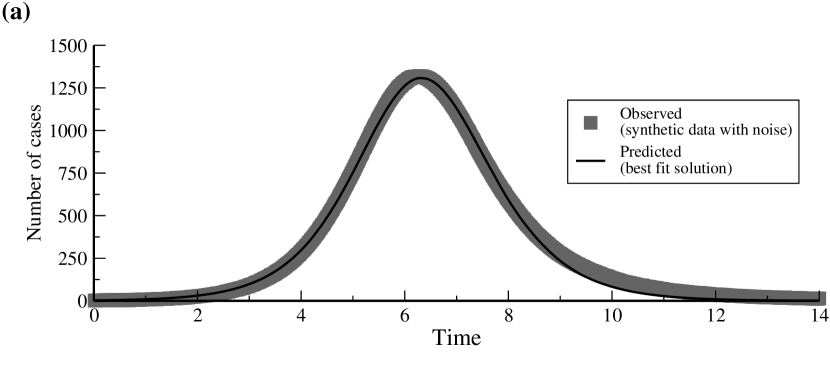
Figure 5: Results obtained using $\theta=2.75\theta_{0}$ as the initial guess in the optimization algorithm, applying the OLS methodology to synthetic data with $n=1,000$ and $\alpha=0.50$. Panel (a) displays the model prediction (solid curve), and the observations (solid squares), respectively. Panel (b) displays the residuals against the model values and panel (c) displays the residuals versus time.

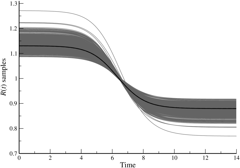
Figure 6: One thousand of the $m=10,000$ effective reproductive number curves (solid gray) constructed using parameters drawn from the 4-multivariate normal distribution $\mathcal{N}_{4}(\hat{\theta}_{OLS},\hat{\Sigma}^{n}_{OLS})$. The curve $\mathcal{R}(t;\hat{\theta}_{OLS})$ is shown in solid black. The curve of the median value of the $\mathcal{R}(t)$ samples, at each $t$, is also shown as a dashed black curve, but is indistinguishable from the curve $\mathcal{R}(t;\hat{\theta}_{OLS})$.

5.2 Synthetic Data with Non-constant Variance Noise

We generated a second synthetic data set with non-constant variance noise. The true value $\theta_{0}$ was fixed, and was used to calculate the numerical solution $z(t_{j};\theta_{0})$. Observations were computed in the following fashion:

$$Y_{j}=z(t_{j};\theta_{0})\left(1+\alpha V_{j}\right),$$ (41)

where the $V_{j}$ are independent random variables with standard normal distribution, and $0<\alpha<1$ denotes a desired percentage. In this way, $var(Y_{j})=[z(t_{j};\theta_{0})\alpha]^{2}$ which is non-constant across the time points $t_{j}$. If the terms $\{v_{j}\}_{j=1}^{n}$ denote a realization of $\{V_{j}\}_{j=1}^{n}$, then a realization of the observation process is denoted by $y_{j}=z(t_{j};\theta_{0})(1+\alpha v_{j})$.

An $n=1,000$ point synthetic data set was constructed with $\alpha=0.075$. The optimization algorithm was initialized with the estimate $\theta=1.10\theta_{0}$. The weights in the normal equations defined by Equation (32), were chosen as $w_{j}=1/z(t_{j};\theta)^{2}$.

Table 4 lists estimates of the parameters and $\mathcal{R}(t)$, together with uncertainty estimates. In the case of $\mathcal{R}(t)$, uncertainty was assessed based on the simulation approach using $m=10,000$ samples of the parameter vector, drawn from $\mathcal{N}_{4}(\hat{\theta}_{GLS},\hat{\Sigma}^{n}_{GLS})$. Figure 7(a) depicts both data and fitted model points, $z(t_{j};\hat{\theta}_{GLS})$, plotted versus $t_{j}$. Figure 7(b) depicts $1,000$ of the $10,000$ $\mathcal{R}(t)$ curves.

Table 4: Estimates from a synthetic data of size $n=1,000$, with non-constant variance using $\alpha=0.075$. The $\mathcal{R}(t)$ sample size is $m=10,000$. The initial guess of the optimization algorithm was $\theta=1.10\theta_{0}$. Each weight in the cost function $L(\theta)$ (see Equation (33)) was equal to $1/z(t_{j};\theta)^{2}$ for $j=1,\dots,n$.

Parameter	True value	Initial guess	Estimate	Standard error
$S_{0}$	3.5000$\times 10^{5}$	3.800$\times 10^{5}$	3.498$\times 10^{5}$	1.375$\times 10^{3}$
$I_{0}$	9.000$\times 10^{1}$	9.900$\times 10^{1}$	9.085$\times 10^{1}$	1.424$\times 10^{0}$
$\tilde{\beta}$	5.000$\times 10^{-6}$	5.500$\times 10^{-6}$	4.954$\times 10^{-6}$	4.411$\times 10^{-8}$
$\gamma$	5.000$\times 10^{-1}$	5.500$\times 10^{-1}$	4.847$\times 10^{-1}$	1.636$\times 10^{-2}$
$L(\hat{\theta}_{GLS})=5.689\times 10^{0}$
$\sigma_{0}^{2}=5.625\times 10^{-3}$			$\hat{\sigma}^{2}_{GLS}=5.712\times 10^{-3}$
Min. $\mathcal{R}(t;\hat{\theta}_{GLS})$			0.132  [0.120,0.146]
Max. $\mathcal{R}(t;\hat{\theta}_{GLS})$			3.576  [3.420,3.753]

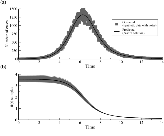
Figure 7: Results from applying the GLS methodology to synthetic data with non-constant variance noise ($\alpha=0.075$), using $n=1,000$ observations. The initial guess for the optimization routine was $\theta=1.10\theta_{0}$. The weights in the cost function were equal to $1/z(t_{j};\theta)^{2}$, for $j=1,\dots,n$. Panel (a) depicts the observed and fitted values and panel (b) displays $1,000$ of the $m=10,000$ $\mathcal{R}(t)$ sample trajectories. Residuals plots are presented in panels (c) and (d): modified residuals versus fitted values in (c) and modified residuals versus time in (d).

Residuals plots are displayed in Figures 7(c) and (d). Because $\alpha v_{j}=(y_{j}-z(t_{j};\theta_{0}))/z(t_{j};\theta_{0})$, by construction of the synthetic data, the residuals analysis focuses on the ratios

$$\frac{y_{j}-z(t_{j};\hat{\theta}_{GLS})}{z(t_{j};\hat{\theta}_{GLS})}$$

which in the labels of Figures 7(c) and (d) are referred to as “Modified residuals”. In Figure 7(c) these ratios are plotted against $z(t_{j};\hat{\theta}_{GLS})$, while Panel (d) displays them versus the time points $t_{j}$. The lack of any discernable patterns or trends in Figure 7(c) and (d) confirms that the errors in the synthetic data set conform to the assumptions made in the formulation of the statistical model of Equation (41). In particular, the errors are uncorrelated and have variance that scales according to the relationship stated above.

6 Analysis of Influenza Outbreak Data

The OLS and GLS methodologies were applied to longitudinal observations of six influenza outbreaks (see Section 2), giving estimates of the parameters and the reproductive number for each season. The number of observations $n$ varies from season to season. The $\mathcal{R}(t)$ sample size was $m=10,000$ in each case. The set of admissible parameters $\Theta$ is defined by the lower and upper bounds listed in Table 5 along with the inequality constraint $S_{0}\tilde{\beta}/\gamma>1$. The bounds in Table 5 were obtained or based on [8, 23, 25] and references therein. For brevity, we only present here the results obtained using data from the 1989-1999 season.

Table 5: Lower and upper bounds on the initial conditions and parameters.

Suitable Range	Unit
1.00$\times 10^{2}$ $<S_{0}<$ 7.00$\times 10^{6}$	people
0.00 $<I_{0}<$ 5.00$\times 10^{3}$	people
7.00$\times 10^{-9}$ $<\tilde{\beta}<$ 7.00$\times 10^{-1}$	weeks-1people-1
$3/7<1/\gamma<$4/7	weeks

6.1 OLS Estimation

In most cases, visual comparison of the trajectory of the best fitting model obtained using OLS and the data points suggests that a good fit has been achieved (Figure 8(a)). The statistics that quantify the uncertainty in the estimated values of the parameters, however, indicate that this may not always be the case. In many cases, the standard errors are of the same order of magnitude as the parameter values themselves, indicating wide error bounds (see Table 6) and suggesting a lack of confidence in the estimates.

We should, however, interpret the statistical results with some caution because the residuals plots (Figure 8(c) and (d)) show clear patterns, indicating that the assumptions of the statistical model may have been violated. For instance, the variance of the residuals appears to increase with the predicted value. There are definite patterns visible in the residuals versus time plot. The temporal correlation of the errors could represent some inadequacy in the way that the dynamic model describes the epidemic process, or an inadequacy in the data set itself.

Another indication of problems in the estimation process comes from the matrix $\chi(\hat{\theta}_{OLS},n)^{T}\chi(\hat{\theta}_{OLS},n)$. The condition number of this matrix is $9.4\times 10^{19}$, indicating that the matrix is close to singular. Calculation of the covariance matrix requires the inversion of this matrix, and, as mentioned above, the asymptotic theory requires that the matrix $\Omega_{0}$, defined as a limit of matrix products of this form, has a non singular limit as $n\rightarrow\infty$. A nearly singular matrix can arise when there is redundancy in the data or when there are problems with parameter identifiability [3, 4].

It is interesting to observe that the estimated values of $\gamma$ frequently fall on the boundary of the feasible region. This may impact the uncertainty analysis, given that the conditions of the asymptotic theory require that the true parameter value lies in the interior of the feasible region. If our estimates commonly fall on the boundary, this could be an indication that the true parameter value may not lie within our feasible region. We return to this issue below, in Section 6.4.

Table 6: Season 1998-1999. Parameter and effective reproductive number estimates obtained using OLS.

Parameter	Estimate	Standard error
$S_{0}$	6.200$\times 10^{3}$	4.514$\times 10^{3}$
$I_{0}$	3.878$\times 10^{-2}$	1.812$\times 10^{-2}$
$\tilde{\beta}$	3.667$\times 10^{-4}$	2.198$\times 10^{-5}$
$\gamma$	1.750$\times 10^{0}$	1.753$\times 10^{0}$
$J(\hat{\theta}_{OLS})=6.357\times 10^{3}$
$\hat{\sigma}^{2}_{OLS}=2.192\times 10^{2}$
Min. $\mathcal{R}(t;\hat{\theta}_{OLS})$	0.752  [0.752,0.824]
Max. $\mathcal{R}(t;\hat{\theta}_{OLS})$	1.299  [1.202,1.300]

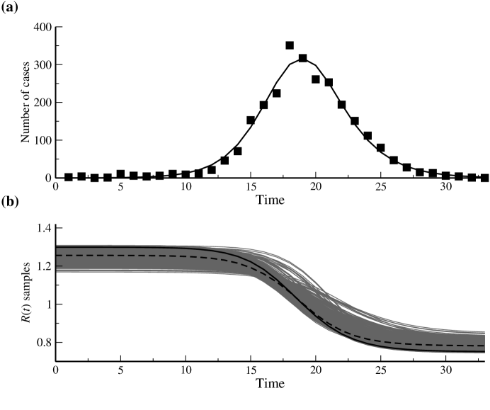
Figure 8: OLS model fits to influenza data from season 1998-1999. Panel (a) depicts the observations (solid squares) and the model prediction (solid curve), respectively. In Panel (b) the samples of the effective reproductive number $\mathcal{R}(t)$ are displayed (grey curves) together with the central estimate $\mathcal{R}(t;\hat{\theta}_{OLS})$ (solid black curve). The dashed black curve depicts the median, at each time point, of the distribution of the $\mathcal{R}(t)$ samples. Panel (c) contains the residuals plotted versus the model prediction. In Panel (d) residuals are plotted against time.

6.2 GLS Estimation

Visual inspection suggests that the model fits obtained using the GLS approach (Figure 9) are even worse than those obtained using OLS. This is somewhat misleading, however, because the weights, defined as $w_{j}=1/[z(t_{j};\theta)]^{2}$, mean that the GLS fitting procedure (unlike visual inspection of the figures) places increased emphasis on datapoints whose model value is small and decreased emphasis on datapoints where the model value is large. If these graphs are, instead, plotted with a logarithmic scale on the vertical axis, an accurate visualization is obtained (Figure 10): multiplicative observation noise on a linear scale becomes constant variance additive observation noise on a logarithmic scale.

As before, however, the parameter estimates have standard errors that are often of the same order of magnitude as the estimates themselves (Table 7). The residuals plots reveal clear patterns and trends (Figure 9(c) and (d)). Temporal trends in the residuals (and visual inspection of the plots depicting the best fitting model and the datapoints) indicate that there are systematic differences between the fitted model and the data. For instance, it appears that the fitted model peaks slightly earlier than the observed outbreak, and, as a result, there are numbers of sequential points where the data lies above or below the model. The modified residuals versus model plot suggests that the variation of the residuals may be decreasing as the model value increases.

The condition number of the matrix $\chi(\hat{\theta}_{GLS},n)^{T}W(\hat{\theta}_{GLS})\chi(\hat{\theta}_{GLS},n)$ is $9.0\times 10^{19}$. This is very similar to that for the OLS estimation, again suggesting caution in interpreting the standard errors.

The modified residuals versus model plot indicates that the $1/z(t_{j};\hat{\theta}_{GLS})^{2}$ weights may have overcompensated for the non-constant variance seen in the OLS residuals. This suggests that it may be appropriate to use weights that vary in a milder fashion, such as $1/z(t_{j};\hat{\theta}_{GLS})$. The model fits that result with these new weights appear, by visual inspection, to provide a more satisfactory fit to the data (Figure 11). Standard errors for the parameter estimates are still large, however (Table 8). Our earlier comment concerning the difficulty of assessing the adequacy of GLS model fits by visual inspection should be borne in mind— see Figure 12 for a more accurate depiction in which square roots of the quantities are plotted so as to transform the errors in which variance scales with the model value into additive errors with constant variance.

The new modified residuals plots, which now focus on the quantities

$$\frac{y_{j}-z(t_{j};\hat{\theta}_{GLS})}{z(t_{j};\hat{\theta}_{GLS})^{1/2}},$$

also appear to exhibit less marked patterns than they did for either OLS or GLS with the $1/z^{2}$ weights (Figures 11(c) and (d)). The condition number for the matrix $\chi(\hat{\theta}_{GLS},n)^{T}W(\hat{\theta}_{GLS})\chi(\hat{\theta}_{GLS},n)$ is $1.3\times 10^{20}$, again suggesting ill-posedness and that the standard errors should be interpreted with caution.

A handful of surprisingly large modified residuals are seen on many occasions, although these often do not appear on our plots because we choose the range on the residuals axis so that the majority of the points can be seen most clearly. The locations of these residuals is noted on the figure caption; we see that they occur during the initial part of the time series, when the numbers of cases are low.

Table 7: Results of GLS estimation applied to influenza data from season 1998-1999, weights equal to $1/z(t_{j};\theta)^{2}$.

Parameter	Estimate	Standard error
$S_{0}$	7.939$\times 10^{3}$	1.521$\times 10^{4}$
$I_{0}$	2.436$\times 10^{-1}$	4.216$\times 10^{-1}$
$\tilde{\beta}$	3.458$\times 10^{-4}$	5.233$\times 10^{-5}$
$\gamma$	2.333$\times 10^{0}$	5.318$\times 10^{0}$
$L(\hat{\theta}_{GLS})=$1.754$\times 10^{1}$
$\hat{\sigma}^{2}_{GLS}=6.047\times 10^{-1}$
Min. $\mathcal{R}(t;\hat{\theta}_{GLS})$	0.843  [0.784,1.018]
Max. $\mathcal{R}(t;\hat{\theta}_{GLS})$	1.177  [1.052,1.252]

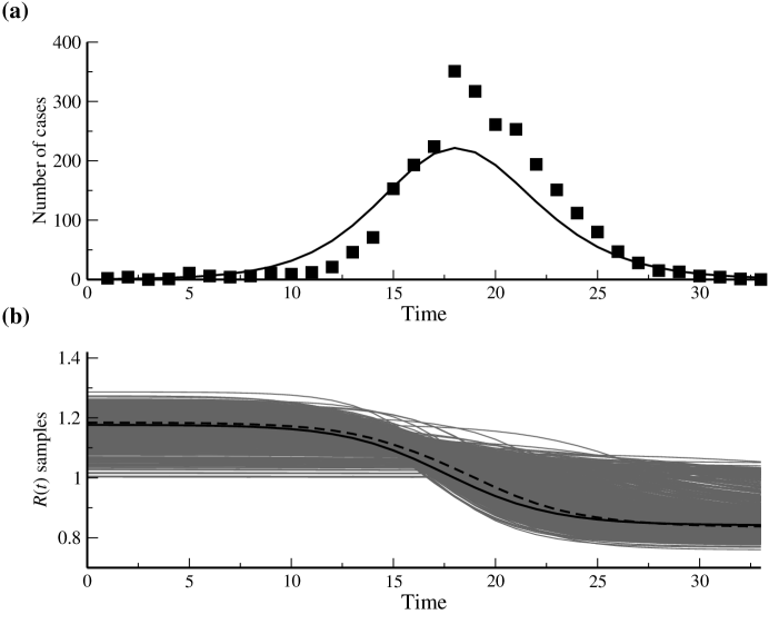
Figure 9: GLS applied to influenza data from season 1998-1999. The weights were taken equal to $1/z(t_{j};\theta)^{2}$. Panel (a) depicts the observations (solid squares) as well as the model prediction (solid curve). In Panel (b) $1,000$ of the $m=10,000$ samples of the effective reproductive number $\mathcal{R}(t)$ are displayed. The solid curve depicts the central estimate $\mathcal{R}(t;\hat{\theta}_{GLS})$ and the dashed curve the median of the $\mathcal{R}(t)$ samples at each point in time. Panel (c) exhibits the modified residuals $(y_{j}-z(t_{j};\hat{\theta}_{GLS}))/z(t_{j};\hat{\theta}_{GLS})$ plotted versus the model predictions, $z(t_{j};\hat{\theta}_{GLS})$. Panel (d) displays the modified residuals plotted against time.

Figure 10: Best fitting model for the 1998-1999 season, obtained using GLS with $1/z(t_{j};\theta)^{2}$ weights. Observations (solid squares) and the model prediction (solid curve) are plotted on a logarithmic scale.

Table 8: Results of GLS estimation applied to the 1998-1999 season influenza data. Weights taken to equal $1/z(t_{j};\theta)$.

Parameter	Estimate	Standard error
$S_{0}$	7.799$\times 10^{3}$	9.269$\times 10^{3}$
$I_{0}$	3.868$\times 10^{-2}$	3.183$\times 10^{-2}$
$\tilde{\beta}$	3.643$\times 10^{-4}$	2.760$\times 10^{-5}$
$\gamma$	2.333$\times 10^{0}$	3.462$\times 10^{0}$
$L(\hat{\theta}_{GLS})=$2.335$\times 10^{2}$
$\hat{\sigma}^{2}_{GLS}=8.051\times 10^{0}$
Min. $\mathcal{R}(t;\hat{\theta}_{GLS})$	0.810   [0.754,0.828]
Max. $\mathcal{R}(t;\hat{\theta}_{GLS})$	1.218  [1.200,1.297]

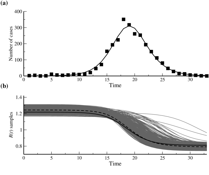
Figure 11: GLS estimation for influenza data from season 1998-1999. Weights equal $1/z(t_{j};\theta)$. Panel (a) depicts the observations (solid squares) as well as the model prediction (solid curve). In Panel (b) $1,000$ of the $m=10,000$ samples of the effective reproductive number $\mathcal{R}(t)$ are displayed, together with the central estimate $\mathcal{R}(t;\hat{\theta}_{GLS}$ (solid curve) and, at each time point, the median of the $\mathcal{R}(t)$ samples (dashed curve). Panel (c) presents the modified residuals $(y_{j}-z(t_{j};\hat{\theta}_{GLS}))/z(t_{j};\hat{\theta}_{GLS})^{1/2}$ versus the model predictions. Panel (d) displays the modified residuals plotted against time. Three modified residuals fall outside the range shown on this graph: their values (and the timepoints at which they arise) are -4.91 (at $t=1$), -7.72 (at $t=2$), and -9.50 (at $t=5$).

Figure 12: Best fitting model for the 1998-1999 season, obtained using GLS with $1/z(t_{j};\theta)$ weights. Square roots of observations (solid squares) and square roots of the model prediction (solid curve) are plotted.

6.3 GLS Estimation Using Truncated Data Sets

It is quite plausible that our description of the error structure of the data is inadequate when the numbers of cases are at low levels. For instance, the reporting process might change as the outbreak starts to take hold (e.g., doctors become more alert to possible flu cases) or comes close to ending. Also, our model is deterministic whereas a real-world epidemic contains stochasticity. Stochastic effects may exhibit a relatively large impact at the start or end of an epidemic, when the numbers of cases are low. It is possible for the infection to undergo extinction, a phenomenon which cannot be captured by the deterministic model. Spatial clustering of cases is also a distinct possibility, particularly during the early stages of an outbreak. This will affect the time course of an outbreak as well as the reporting process: clustering of cases may well increase the reporting noise if cases in a cluster tend to get reported together (e.g., a cluster occurs within an area where many isolates are sent to the CDC) or not reported together (e.g., a cluster occurs in an area that has poorer coverage in the reporting process).

Indeed, examination of one of the influenza time series plotted on either a logarithmic or square root scale (Figures 10 or 12) indicates that both the start and end of the time series are problematic. The fit of the model is clearly poorer over these parts of the time series, which correspond to the times when the observed values are small.

Both forms of the weights (inversely proportional to the square of the predicted incidence or inversely proportional to the predicted incidence) mean that errors at these small values have considerable impact on the cost function, and hence on the GLS estimation process, although this is less of a concern for the $1/z$ weights.

Another issue that has been raised by studies of parameter estimation in biological situations concerns redundancy in information measured when a system is close to its equilibrium [4]. This might be a relevant issue for the final part of the outbreak data as there is often a period lasting ten or more weeks when there are few cases.

We investigated whether the removal of the lowest valued points from the data sets would improve the fitting process. We constructed truncated data sets by considering only the period between the time when the number of isolates first reached ten at the start of the outbreak and first fell below ten at the end of the outbreak. As a notational convenience, we refer to the numbers of susceptibles and infectives at the start of the first week of the truncated data set as $S_{0}$ and $I_{0}$, even though these times no longer correspond to the start of the influenza season. (For example, in Figures 13 and 14, $S_{0}$ and $I_{0}$ refer to the state of the system at $t=8$.)

Comparing Tables 7 and 9, which arise from GLS estimation with $1/z^{2}$ weights, we see that the standard errors for the parameter estimates have decreased. This decrease occurs even though the number of points in the data set has fallen from 35 to 23, causing the factor $1/(n-4)$ that appears in Equation (37) to increase by $80\%$. The corresponding residuals plots (see Figure 13(b) and (c)) provide no evidence that the assumptions of the statistical model are invalid. The condition number of the matrix $\chi(\hat{\theta}_{GLS},n)^{T}W(\hat{\theta}_{GLS})\chi(\hat{\theta}_{GLS},n)$ is $2.4\times 10^{19}$.

A similar result is seen in the $1/z$ weights case. We remark that we no longer have the extreme outlier residuals. The condition number of the matrix $\chi(\hat{\theta}_{GLS},n)^{T}W(\hat{\theta}_{GLS})\chi(\hat{\theta}_{GLS},n)$ is $9.2\times 10^{19}$.

Truncating the data sets has helped considerably with the GLS estimation process, although the large condition numbers still are cause for caution with the standard errors.

Truncation of the data set had little effect on the parameter estimates obtained using OLS (results not shown), except that the values of $S_{0}$ and $I_{0}$ were changed because they refer to a later initial time, as discussed above. Standard errors for the OLS estimates were higher than for the full data set, as should be expected given the reduced number of data points.

Table 9: Estimation results from GLS, with weights $1/z(t_{j};\theta)^{2}$, applied to truncated influenza data set for season 1998-1999.

Parameter	Estimate	Standard error
$S_{0}$	7.458$\times 10^{3}$	5.936$\times 10^{3}$
$I_{0}$	1.758$\times 10^{0}$	1.279$\times 10^{0}$
$\tilde{\beta}$	3.828$\times 10^{-4}$	2.069$\times 10^{-5}$
$\gamma$	2.333$\times 10^{0}$	2.331$\times 10^{0}$
$L(\hat{\theta}_{GLS})=$9.475$\times 10^{-1}$
$\hat{\sigma}^{2}_{GLS}=5.573\times 10^{-2}$
Min. $\mathcal{R}(t;\hat{\theta}_{GLS})$	0.808  [0.745,0.820]
Max. $\mathcal{R}(t;\hat{\theta}_{GLS})$	1.223  [1.211,1.311]

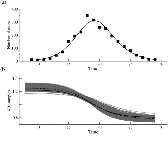
Figure 13: Model fits obtained using GLS on truncated influenza data from season 1998-1999, weights equal to $1/z(t_{j};\theta)^{2}$. Panel (a) depicts the observations (solid squares) as well as the model prediction (solid curve). Panel (b) displays $1,000$ of the $m=10,000$ samples of the effective reproductive number, together with the central estimate $\mathcal{R}(t;\hat{\theta}_{GLS})$ (solid curve), and the median of the $\mathcal{R}(t)$ samples at each point in time (dashed curve). Panel (c) displays the modified residuals versus the model predictions. In Panel (d) modified residuals are plotted against time.

Table 10: Estimation results from GLS, with weights $1/z(t_{j};\theta)$, applied to truncated influenza data set for season 1998-1999.

Parameter	Estimate	Standard error
$S_{0}$	6.017$\times 10^{3}$	3.287$\times 10^{3}$
$I_{0}$	2.091$\times 10^{0}$	9.483$\times 10^{-1}$
$\tilde{\beta}$	3.797$\times 10^{-4}$	1.774$\times 10^{-5}$
$\gamma$	1.750$\times 10^{0}$	1.317$\times 10^{0}$
$L(\hat{\theta}_{GLS})=$3.872$\times 10^{1}$
$\hat{\sigma}^{2}_{GLS}=2.277\times 10^{0}$
Min. $\mathcal{R}(t;\hat{\theta}_{GLS})$	0.750  [0.748,0.819]
Max. $\mathcal{R}(t;\hat{\theta}_{GLS})$	1.306  [1.212,1.308]

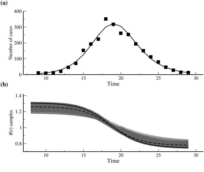
Figure 14: Model fits obtained using GLS on truncated influenza data from season 1998-1999, weights equal to $1/z(t_{j};\theta)$. Panel (a) shows the observations (solid squares) as well as the model prediction (solid curve). In Panel (b) $1,000$ of the $m=10,000$ samples of the effective reproductive number $\mathcal{R}(t)$ are displayed together with the central estimate $\mathcal{R}(t;\hat{\theta}_{GLS})$ (solid curve) and the median of the $\mathcal{R}(t)$ samples at each time point (dashed curve). Panel (c) shows the modified residuals versus the model prediction. In panel (d), each modified residual is displayed versus the observation time point.

6.4 Estimation for a Reduced Parameter Set

The preceding results indicate that there are difficulties in estimating the parameter $\gamma$, as witnessed by the number of situations in which the estimate lies on the boundary of the feasible parameter region. Because $\gamma$ is the one parameter for which we can obtain reasonably reliable estimates without the need to fit a model to an incidence time series [8, 23], we fix its value and investigate estimation for a reduced three parameter problem. In all of what follows, we apply the estimation methodology to the truncated data sets, as discussed in the previous section.

We use a fixed infectious period of four days, i.e., $1/\gamma=4{\rm\ days\ }=4/7{\rm\ weeks}$, and estimate the parameter vector $\theta=(S_{0},I_{0},\tilde{\beta})$ using the OLS approach and the GLS approach with weights $w_{j}=1/[z(t_{j};\theta)]^{2}$ or $w_{j}=1/[z(t_{j};\theta)]$.

Estimation for the reduced parameter set leads to model fits that are not so different from those obtained using the full ($p=4$) set of parameters in $\theta$. For example, for the truncated data set from the 98-99 season, with weights equal to $1/z(t_{j};\theta)$, we have $L(\hat{\theta}_{GLS})=38.72$ for the full parameter set (Table 10) while $L(\hat{\theta}_{GLS})=38.72$ for the reduced parameter set (Table 13). The standard errors of the parameters, however, are smaller for the reduced parameter set: the three standard errors for the estimates of $S_{0}$, $I_{0}$ and $\tilde{\beta}$ are $3.287\times 10^{3}$, $9.483\times 10^{-1}$ and $1.774\times 10^{-5}$, respectively, for the full parameter set, while they are $2.171\times 10^{2}$, $3.174\times 10^{-1}$ and $1.547\times 10^{-5}$ for the reduced set.

The condition numbers of the matrices $\chi(\hat{\theta}_{GLS},n)^{T}W(\hat{\theta}_{GLS})\chi(\hat{\theta}_{GLS},n)$ are $4.5\times 10^{16}$ and $4.2\times 10^{16}$ for the $1/z^{2}$ and $1/z$ weights, respectively. The increased precision of the estimates here likely results from identifiability issues in the estimation problem for the full set of model parameters.

Table 11: Estimation of three epidemiological parameters. Results obtained by applying OLS to truncated influenza data set from season 1998-1999.

Parameter	Estimate	Standard error
$S_{0}$	6.134$\times 10^{3}$	3.329$\times 10^{2}$
$I_{0}$	2.442$\times 10^{0}$	5.435$\times 10^{-1}$
$\tilde{\beta}$	3.707$\times 10^{-4}$	2.348$\times 10^{-5}$
$J(\hat{\theta}_{OLS})=$6.131$\times 10^{3}$
$\hat{\sigma}^{2}_{OLS}=3.406\times 10^{2}$
Min. $\mathcal{R}(t;\hat{\theta}_{OLS})$	0.754  [0.744,0.787]
Max. $\mathcal{R}(t;\hat{\theta}_{OLS})$	1.299  [1.258,1.314]

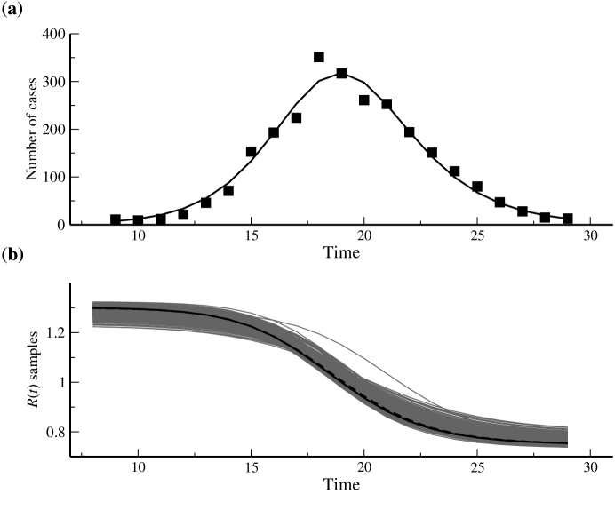
Figure 15: Estimation of three epidemiological parameters using OLS on a truncated data set from the 1998-1999 influenza season. Panel (a) depicts the observations (solid squares) as well as the model prediction (solid curve). In Panel (b) $1,000$ of the $m=10,000$ samples of the effective reproductive number $\mathcal{R}(t)$ are displayed, together with the central estimate $\mathcal{R}(t;\hat{\theta}_{OLS})$ (solid curve) and the median of the $\mathcal{R}(t)$ samples at each time point (dashed curve). Panel (c) exhibits the residuals $y_{j}-z(t_{j};\hat{\theta}_{OLS})$ versus the model predictions $z(t_{j};\hat{\theta}_{OLS})$. In Panel (d) each residual is displayed versus the observation time point $t_{j}=j$, for $j=1\dots,n$.

Table 12: Estimation of three epidemiological parameters. Results obtained by applying GLS, with weights equal to $1/z(t_{j};\theta)^{2}$, to truncated influenza data from season 1998-1999.

Parameter	Estimate	Standard error
$S_{0}$	$5.985\times 10^{3}$	$3.226\times 10^{2}$
$I_{0}$	$2.148\times 10^{0}$	2.890$\times 10^{-1}$
$\tilde{\beta}$	3.808$\times 10^{-4}$	$1.979\times 10^{-5}$
$L(\hat{\theta}_{GLS})=9.880\times 10^{-1}$
$\hat{\sigma}^{2}_{GLS}=5.489\times 10^{-2}$
Min. $\mathcal{R}(t;\hat{\theta}_{GLS})$	0.752  [0.740,0.774]
Max. $\mathcal{R}(t;\hat{\theta}_{GLS})$	1.302  [1.274,1.320]

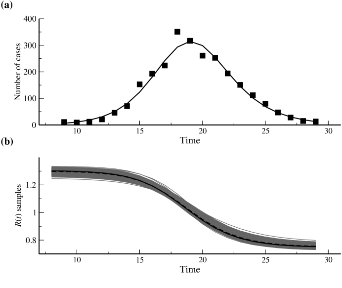
Figure 16: Estimation of three epidemiological parameters, using truncated data from influenza season 1998-1999 and GLS with each weight equal to $1/z(t_{j};\theta)^{2}$ for $j=1,\dots,n$. Panel (a) depicts the observations (solid squares) as well as the model prediction (solid curve). In Panel (b) $1,000$ of the $m=10,000$ samples of the effective reproductive number $\mathcal{R}(t)$ are displayed. The solid curve depicts the central estimate $\mathcal{R}(t;\hat{\theta}_{GLS})$ and, at each time point, the dashed curve depicts the median of the $\mathcal{R}(t)$ samples. Panel (c) exhibits the modified residuals $(y_{j}-z(t_{j};\hat{\theta}_{GLS}))/z(t_{j};\hat{\theta}_{GLS})$ versus the model predictions $z(t_{j};\hat{\theta}_{GLS})$. In Panel (d) each modified residual is displayed versus the observation time point $t_{j}=j$, for $j=1\dots,n$.

Table 13: Estimation of three epidemiological parameters. Results obtained by applying GLS, with weights equal to $1/z(t_{j};\theta)$, to the truncated influenza data set from season 1998-1999.

Parameter	Estimate	Standard error
$S_{0}$	6.017$\times 10^{3}$	2.171$\times 10^{2}$
$I_{0}$	$2.090\times 10^{0}$	$3.174\times 10^{-1}$
$\tilde{\beta}$	3.798$\times 10^{-4}$	1.547$\times 10^{-5}$
$L(\hat{\theta}_{GLS})=$3.872$\times 10^{1}$
$\hat{\sigma}^{2}_{GLS}=2.151\times 10^{0}$
Min. $\mathcal{R}(t;\hat{\theta}_{GLS})$	0.750  [0.739,0.767]
Max. $\mathcal{R}(t;\hat{\theta}_{GLS})$	1.306  [1.283,1.321]

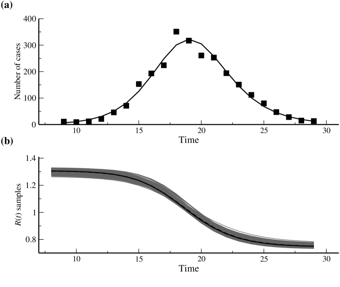
Figure 17: Estimation of three epidemiological parameters using truncated influenza data from season 1998-1999. GLS was used, with each weight equal to $1/z(t_{j};\theta)$ for $j=1,\dots,n$. Panel (a) depicts the observations (solid squares) as well as the model prediction (solid curve). In Panel (b) $1,000$ of the $m=10,000$ samples of the effective reproductive number $\mathcal{R}(t)$ are displayed. Also shown are the central estimate $\mathcal{R}(t;\hat{\theta}_{GLS})$ (solid curve) together with the median of the $\mathcal{R}(t)$ samples (dashed curve). Panel (c) exhibits the modified residuals $(y_{j}-z(t_{j};\hat{\theta}_{GLS}))/z(t_{j};\hat{\theta}_{GLS})^{\frac{1}{2}}$ versus the model predictions $z(t_{j};\hat{\theta}_{GLS})$. In Panel (d) each modified residual is displayed versus the observation time point $t_{j}=j$, for $j=1\dots,n$.

7 Discussion

We have presented parameter estimation methodologies that, using sensitivity analysis and asymptotic statistical theory, also provide measures of uncertainty for the estimated parameters. The techniques were illustrated using synthetic data sets, and it was seen that they can perform very well with reasonable data sets. Even within the ideal situation provided by synthetic data, potential problems of the approach were identified. Worringly, these problems were not apparent from inspection of the uncertainty estimates (standard errors) alone. However, these problems were revealed by examination of model fit diagnostic plots, constructed in terms of the residuals of the fitted model. These results argue strongly for the routine use of uncertainty estimation, together with careful examination of residuals plots when using SIR-type models with surveillance data.

The statistical methodology presented here only addresses the impact of observation error on parameter estimation. While the approach can handle different statistical models for the observation process, it does assume that we have a model that correctly describes the behavior of the system, albeit for an unknown value of the parameter vector. The methodology does not examine the effect of mis-specification of the model. It is well-known that this effect can dwarf the uncertainty that arises from observation error [24]. Examination of residuals plots, however, can identify systematic deviations between the behavior of the model and the data.

Application of the least squares approaches to the influenza isolate data gave mixed results. Estimates of the effective reproductive number were in broad agreement with results obtained in other studies (see Table 14). While apparently reasonable fits were obtained in some instances, the uncertainty analyses highlighted situations in which visual inspection suggested that a good fit had been obtained but for which estimated parameters had large uncertainties. Residuals plots showed that error variance may not have been constant (i.e., observation noise was not simply additive), but more likely scaled according to either the square of the fitted value (i.e., relative measurement error) or the fitted value itself. The potentially large impact of errors at low numbers of cases on the GLS estimation process was clearly observed.

Temporal trends were observed in the residuals plots, indicative of systematic differences between the behavior of the SIR model and the data. Potential sources of these differences include inadequacies of the model to describe the process underlying the data and issues with the reliability of the data itself, particularly in the light of the health warning attached to the data by the CDC. (We emphasize, however, that our use of these data sets should be seen as only an illustration of the approach.)

Sophisticated mathematical and statistical algorithms and analyses can be utilized to fit SIR-type epidemiological models to surveillance data. Good quality data is required if this approach is to be successful. In many instances, however, the available surveillance data is most likely inadequate to validate the SIR model with any degree of confidence. This is likely to be true in much of the modeling efforts for epidemics where the data collection process has inadequacies.

Table 14: Comparison between reproductive number estimates across studies of interpandemic influenza. In this table $\mathcal{R}_{0}$ stands for the basic reproductive number (naive population), while $\max(\mathcal{R}(t))$ denotes the initial effective reproductive number in a non-naive population.

Studies of interpandemic influenza	Estimates
Bonabeau et al. [5]	$1.70\leq\mathcal{R}_{0}\leq 3.00$
Chowell et al. [10]	$1.30\leq\max(\mathcal{R}(t))\leq 1.50$
Dushoff et al. [15]	$4.00\leq\mathcal{R}_{0}\leq 16.00$
Flahault et al. [18]	$\mathcal{R}_{0}=1.37$
Spicer & Lawrence [28]	$1.46\leq\mathcal{R}_{0}\leq 4.48$
Viboud et al. [31]	$1.90\leq\max(\mathcal{R}(t))\leq 2.50$

8 Acknowledgments

This material was based upon work supported by the Statistical and Applied Mathematical Sciences Institute (SAMSI postdoctoral fellowship to A. C.-A.) which is funded by the National Science Foundation under Agreement No. DMS-0112069. Any opinions, findings, and conclusions or recommendations expressed in this material are those of the authors and do not necessarily reflect the views of the National Science Foundation.

References

- [1] R. Anderson and R. May, Infectious Diseases of Humans: Dynamics and Control, Oxford University Press, 1991.
- [2] P. Bai, H. T. Banks, S. Dediu, A. Y. Govan, M. Last, A. L. Lloyd, H. K. Nguyen, M. S. Olufsen, G. Rempala, and B. D. Slenning, Stochastic and deterministic models for agricultural production networks, Math. Biosci. Eng. 4 (2007), 373-402.
- [3] H. T. Banks, M. Davidian, J. R. Samuels, Jr., and K. L. Sutton An inverse problem statistical methodology summary. Center for Research in Scientific Computation Technical Report CRSC-TR08-1, NCSU, Raleigh NC. 2008; in Mathematical and Statistical Estimation Approaches in Epidemiology, (G. Chowell, et. al., eds.), Springer, New York, to appear.
- [4] H. T. Banks, S. L. Ernstberger and S. L. Grove, Standard errors and confidence intervals in inverse problems: Sensitivity and associated pitfalls. Center for Research in Scientific Computation. Technical Report CRSC-TR06-10, NCSU, Raleigh NC. 2006; J. Inv. Ill-posed Problems 15 (2006), 1-18.
- [5] E. Bonabeau, L. Toubiana, and A. Flahault, The geographical spread of influenza, Proc. R. Soc. Lond. B 265 (1998), 2421-2425.
- [6] F. Brauer and C. Castillo-Chávez, Mathematical Models in Population Biology and Epidemiology, Springer, New York, 2001.
- [7] R. J. Carroll, C. F. Wu, and D. Ruppert, The effect of estimating weights in weighted least squares, J. Am. Stat. Assoc. 83 (1988), 1045-1054.
- [8] S. Cauchemez, F. Carrat, C. Viboud, A. J. Valleron, and P. Y. Boelle, A Bayesian MCMC approach to study transmission of influenza: application to household longitudinal data, Stat. Med. 23 (2004), 3469-3487.
- [9] Centers for Disease Control and Prevention (CDC), Flu activity, reports and surveillance methods in the United States, website: http://www.cdc.gov/flu/weekly/fluactivity.htm, accessed on April 7, 2006.
- [10] G. Chowell, M. A. Miller, and C. Viboud, Seasonal influenza in the United States, France, and Australia: transmission and prospects for control, Epidemiol. Infect. 136 (2008), 852-864.
- [11] R. B. Couch and J. A. Kasel, Immunity to influenza in man, Ann. Rev. Microbiol. 31 (1983), 529-549.
- [12] J. B. Cruz, Jr., ed., System Sensitivity Analysis, Dowden, Hutchinson & Ross, Inc., Stroudsberg, PA, 1973.
- [13] M. Davidian and D. M. Giltinan, Nonlinear Models for Repeated Measurement Data, Chapman & Hall, Boca Raton, 1995.
- [14] K. Dietz, The estimation of the basic reproduction number for infectious diseases, Stat. Methods Med. Res. 2 (1993), 23-41.
- [15] J. Dushoff, J. B. Plotkin, S. A. Levin, and D. J. D. Earn, Dynamical resonance can account for seasonality of influenza epidemics, Proc. Natl. Acad. Sci. USA 101 (2004), 16915-16916.
- [16] M. Eslami, Theory of Sensitivity in Dynamic Systems: An Introduction, Springer-Verlag, New York, NY, 1994.
- [17] N. M. Ferguson, A. P. Galvani, and R. M. Bush, Ecological and immunological determinants of influenza evolution, Nature 422 (2003), 428-433.
- [18] A. Flahault, S. Letrait, P. Blin, S. Hazout, J. Menares, and A. J. Valleron, Modeling the 1985 influenza epidemic in France, Stat. Med. 7 (1988), 1147-1155.
- [19] P. M. Frank, Introduction to System Sensitivity Theory, Academic Press, New York, NY, 1978.
- [20] H. Hethcote, The mathematics of infectious diseases, SIAM Rev. 42 (2000), 599-653.
- [21] M. Kleiber, H. Antunez, T. D. Hien, and P. Kowalczyk, Parameter Sensitivity in Nonlinear Mechanics: Theory and Finite Element Computations, John Wiley & Sons, Chichester, 1997.
- [22] J. C. Lagarias, J. A. Reeds, M. H. Wright, and P. E. Wright, Convergence properties of the Nelder-Mead simplex method in low dimensions, SIAM J. Optimiz. 9 (1999), 112-147.
- [23] I. M. Longini, J. S. Koopman, A. S. Monto, and J. P. Fox, Estimating household and community transmission parameters for influenza, Am. J. Epidemiol. 115 (1982), 736-751.
- [24] A. L. Lloyd, The dependence of viral parameter estimates on the assumed viral life cycle: limitations of studies of viral load data, Proc. R. Soc. Lond. B. 268 (2001), 847-854.
- [25] M. Nuno, G. Chowell, X. Wang, C. Castillo-Chávez, On the role of cross-immunity and vaccination in the survival of less-fit flu strains, Theor. Pop. Biol. 71 (2007), 20-29.
- [26] A. Saltelli, K. Chan, and E. M. Scott, eds., Sensitivity Analysis, John Wiley & Sons, Chichester, 2000.
- [27] G. A. F. Seber and C. J. Wild, Nonlinear Regression, John Wiley & Sons, Chichester, 2003.
- [28] C. C. Spicer and C. J. Lawrence, Epidemic influenza in Greater London, J. Hyg. Camb. 93 (1984), 105-112.
- [29] W. Thompson, D. Shay, E. Weintraub, L. Brammer, N. Cox, L. Anderson, and K. Fukuda, Mortality associated with influenza and respiratory syncytial virus in the United States, JAMA 289 (2003), 179-186.
- [30] US Department of Health and Human Services, website: http://www.pandemicflu.gov/general/historicaloverview.html, accessed on December 16, 2006.
- [31] C. Viboud, T. Tam, D. Fleming, A. Handel, M. Miller, and L. Simonsen, Transmissibility and mortality impact of epidemic and pandemic influenza, with emphasis on the unusually deadly 1951 epidemic, Vaccine 24 (2006), 6701-6707.